Fractal Calculus of Functions on Cantor Tartan Spaces

Abstract

In this manuscript, integrals and derivatives of functions on Cantor tartan spaces are defined. The generalisation of standard calculus, which is called $F^{\eta }$-calculus, is utilised to obtain definitions of the integral and derivative of functions on Cantor tartan spaces of different dimensions. Differential equations involving the new derivatives are solved. Illustrative examples are presented to check the details.

1. Introduction

Fractal shapes and objects are frequently seen in nature, e.g., clouds, mountains, coastlines, the human body, and so on. The geometry of fractals has been studied a great deal, e.g., see [1,2,3,4]. Analysis of fractals has been established using various different methods—such as fractional calculus, probability theory, measure theory, fractional spaces, and time scale theory—by many researchers and has found many applications [5,6,7,8,9,10,11,12,13,14,15].

Fractional calculus, which involves derivatives with arbitrary orders, has been applied to processes with fractal structures [16,17,18]. Fractional derivatives have non-locality properties, which makes them suitable to model processes with memory effects in statistical mechanics, and provide mathematical models for non-conservative systems in classical mechanics [19,20,21,22,23,24,25,26].

Anomalous diffusion processes have been modelled using fractals, where the concepts of fractal invariance and equivalence can be used to formulate fractional quantum mechanics [27]. These models behave differently from fractional models for anomalous diffusion, due to the locality of the fractal models [28,29,30,31]. This also covers sub-diffusion and super-diffusion, in view of different random walks [32,33].

Fractal geometry has also been used in antenna design: specifically, the idea of space-filling curves is useful in designing miniaturised antenna elements, because it enables long wires to be fitted into a small volume [34,35].

Laminar flow of a fractal fluid in a cylindrical tube has been studied using homogeneous flow in a fractional-dimensional space [36,37]. On the Cantor cubes, Maxwell’s equations were obtained using fractal vector calculus and used to build a model of fractal continuum electrodynamics; as an application, the electric field due to Cantor dust was obtained [38].

Recently, an algorithmic model called $F^{\eta }$-calculus was suggested and applied to model some physical processes [39,40,41,42]. The advantage of this model is that it can be used in contexts where the usual calculus cannot be applied, e.g., for functions with fractal support that are not differentiable or integrable in the usual sense.

This manuscript is structured as follows. In Section 2, we set up the notation and terminology of $F^{\eta }$-calculus on fractals embedded in ${\Re }^2$ and verify some basic properties of this new $F^{\eta }$-calculus. In Section 3, we study some example functions on the Cantor tartan using these suggested definitions. In Section 4, we consider the diffusion equation on the Cantor tartan, as another example. Section 5 is devoted to the conclusion.

2. Terminology and Notations

In this section, we review and define the basic tools we need in our work.

Fractals are sets with self-similar properties such that their fractal dimension exceeds their topological dimension. We shall consider calculus on the Cantor tartan, a space $\mathbb{F}$, which is established by first taking the Cartesian product F of a Cantor set and a continuous interval and then taking the union of two orthogonal copies of this F. In other words:

$$\begin{array}{c}\mathbb{F}=F_1\cup F_2\subset {[0,1]}^2,\\ F_1=C\times [0,1],F_2=[0,1]\times C,\end{array}$$

where $C\subset [0,1]$ is a Cantor set of some fractal dimension less than one [2]. We can consider intersections of the Cantor tartan $\mathbb{F}$ with a box $I=[a_1,a_2]\times [b_1,b_2],a_1,a_2,b_1,b_2\in \Re$. The sketches in Figure 1 show finite iterations (approximations to fractal space) of the Cantor tartan with different dimensions.

Definition 1

(Flag functions and subdivisions). The flag function for the Cantor tartan $\mathbb{F}=F_1\cup F_2\subset {\Re }^2$ and the box $I=[a_1,a_2]\times [b_1,b_2]$, which is denoted by $\Psi (\mathbb{F},I)$, is defined as follows:

$$\Psi (\mathbb{F},I)=\left\{\begin{array}{c}1,if\mathbb{F}\cap I\ne \varnothing ,\hfill \\ 0,otherwise.\hfill \end{array}\right.$$

(1)

A subdivision of the box $I=[a_1,a_2]\times [b_1,b_2]$ is a set of the following form:

$${\mathbb{P}}_{[a_1,a_2]\times [b_1,b_2]}=\{a_1=x_0,x_1,x_2,\dots ,x_n=a_2\}\times \{b_1=y_0,y_1,y_2,\dots ,y_m=b_2\},$$

(2)

where × denotes the Cartesian product.

Definition 2

(Mass functions). For a Cantor tartan space $\mathbb{F}$ and a subdivision ${\mathbb{P}}_{[a_1,a_2]\times [b_1,b_2]}$ as above and for any $\eta ,ϵ$ between zero and one, we define:

$${\sigma }^{\eta ,ϵ}\left(\mathbb{F},{\mathbb{P}}_{[a_1,a_2]\times [b_1,b_2]}\right)=\sum _{j=1}^m\sum _{i=1}^n\Gamma (\eta +1)\Gamma (ϵ+1){(x_i-x_{i-1})}^{\eta }{(y_j-y_{j-1})}^{ϵ}\Psi (\mathbb{F},[x_{i-1},x_i]\times [y_{j-1},y_j]).$$

(3)

For a Cantor tartan space $\mathbb{F}$ and box $I=[a_1,a_2]\times [b_1,b_2]$ as above, and for any $\eta ,ϵ$ between zero and one, the mass function ${\gamma }^{\eta ,ϵ}(\mathbb{F},a_1,a_2,b_1,b_2)$ is defined as:

$${\gamma }^{\eta ,ϵ}(\mathbb{F},a_1,a_2,b_1,b_2)=\underset{\delta \to 0}{lim}\left[\underset{{\mathbb{P}}_{[a_1,a_2]\times [b_1,b_2]}:|\mathbb{P}|\le \delta }{inf}{\sigma }^{\eta ,ϵ}\left(\mathbb{F},{\mathbb{P}}_{[a_1,a_2]\times [b_1,b_2]}\right)\right],$$

(4)

where $|\mathbb{P}|$ is defined as:

$$|\mathbb{P}|=\underset{1\le i\le n,1\le j\le m}{max}(x_i-x_{i-1})\times (y_j-y_{j-1}).$$

(5)

Lemma 1.

For a Cantor tartan space $\mathbb{F}$ and fixed $\eta ,ϵ\in (0,1)$ as above, the mass function ${\gamma }^{\eta ,ϵ}(\mathbb{F},a_1,a_2,b_1,b_2)$ is continuous and monotonically increasing in each of the four real variables $a_1$, $a_2$, $b_1$, $b_2$.

Proof. 

This is similar to the one-dimensional case, which was proven in [39] (Theorem 7) and [39] (Lemma 6), respectively. □

Lemma 2.

For a Cantor tartan space $\mathbb{F}$ and fixed $\eta ,ϵ\in (0,1)$ as above, the mass function ${\gamma }^{\eta ,ϵ}(\mathbb{F},a_1,a_2,b_1,b_2)$ is zero for any $a_1,a_2,b_1,b_2$ such that $\mathbb{F}$ does not intersect $(a_1,a_2)\times (b_1,b_2)$.

Proof. 

If $\mathbb{F}$ does not intersect $I=[a_1,a_2]\times [b_1,b_2]$, then the flag function $\Psi (\mathbb{F},[x_{i-1},x_i]\times [y_{j-1},y_j])$ is zero for all $i,j$, so we are done.

Therefore, we assume that $\mathbb{F}$ intersects the boundary of I. Fix $\nu >0$; we aim to find a subdivision $\mathbb{P}={\mathbb{P}}_{[a_1,a_2]\times [b_1,b_2]}$ such that ${\sigma }^{\eta ,ϵ}\left(\mathbb{F},\mathbb{P}\right)<\nu$. In order to do this, we choose $\mathbb{P}$ such that, in the notation of (2), we have:

$$\begin{array}{cc}\hfill {(x_1-x_0)}^{\eta }{(y_j-y_{j-1})}^{ϵ}& <\frac{\nu }{m\Gamma (\eta +1)\Gamma (ϵ+1)},\hfill \\ \hfill {(x_n-x_{n-1})}^{\eta }{(y_j-y_{j-1})}^{ϵ}& <\frac{\nu }{m\Gamma (\eta +1)\Gamma (\nu +1)},\hfill \\ \hfill {(x_i-x_{i-1})}^{\eta }{(y_1-y_0)}^{ϵ}& <\frac{\nu }{n\Gamma (\eta +1)\Gamma (ϵ+1)},\hfill \\ \hfill {(x_i-x_{i-1})}^{\eta }{(y_m-y_{m-1})}^{ϵ}& <\frac{\nu }{n\Gamma (\eta +1)\Gamma (ϵ+1)},\hfill \end{array}$$

for all i and j. Thus, by the definition (3), we have ${\sigma }^{\eta ,ϵ}\left(\mathbb{F},\mathbb{P}\right)<\nu$. Since $ϵ>0$ was arbitrary, this is enough to prove ${\gamma }^{\eta ,ϵ}(\mathbb{F},a_1,a_2,b_1,b_2)=0$ as required. □

Definition 3

(Integral staircase functions). The integral staircase function $S_{\mathbb{F}}^{\eta ,ϵ}(x,y)$ for the Cantor tartan $\mathbb{F}$ is defined by:

$$S_{\mathbb{F}}^{\eta ,ϵ}(x,y)=\left\{\begin{array}{c}{\gamma }^{\eta ,ϵ}(\mathbb{F},a_0,b_0,x,y),ifx\ge a_0,y\ge b_0;\hfill \\ -{\gamma }^{\eta ,ϵ}(\mathbb{F},a_0,b_0,x,y),otherwise,\hfill \end{array}\right.$$

(6)

where $a_0,c_0$ are real numbers chosen according to convenience (e.g., often we might choose $a_0=c_0=0$). The integral staircase functions for different Cantor tartan spaces with different dimensions are plotted in Figure 2.

Corollary 1.

For a Cantor tartan space $\mathbb{F}$ and fixed $\eta ,ϵ\in (0,1)$ as above, the integral staircase function $S_{\mathbb{F}}^{\eta ,ϵ}(x,y)$ is continuous and monotonically increasing in each of the two real variables x, y.

Proof. 

This follows directly from Lemma 1 and the definition of the integral staircase function. □

Definition 4

(γ2-dimension). The ${\gamma }_2$-dimension of $\mathbb{F}\cap ([a_1,a_2]\times [b_1,b_2])$ is given by:

$$\begin{array}{ccc}\hfill {dim}_{{\gamma }_2}(\mathbb{F}\cap ([a_1,a_2]\times [b_1,b_2]))& =& inf\{max\{\eta ,ϵ\}:{\gamma }^{\eta ,ϵ}(\mathbb{F},a_1,a_2,b_1,b_2)=0\}\hfill \\ & =& sup\{max\{\eta ,ϵ\}:{\gamma }^{\eta ,ϵ}(\mathbb{F},a_1,a_2,b_1,b_2)=\infty \}.\hfill \end{array}$$

(7)

Lemma 3.

The Hausdorff dimension is finer than the ${\gamma }_2$-dimension.

Proof. 

Here, we must prove that ${dim}_H(\mathbb{F})\le {dim}_{{\gamma }_2}(\mathbb{F})$ for any Cantor tartan $\mathbb{F}$ as above.

We use the notation $H_{\delta }^{\gamma }(\mathbb{F})$ for the coarse grained Hausdorff measure and $H^{\gamma }(\mathbb{F})$ for the Hausdorff measure. For any subdivision ${\mathbb{P}}_{[a_1,a_2]\times [b_1,b_2]}$ with $|\mathbb{P}|\le \delta$, we have:

$${\sigma }^{\eta ,ϵ}[\mathbb{F},\mathbb{P}]\ge \Gamma (\eta +1)\Gamma (ϵ+1)H_{\delta }^{\gamma }(\mathbb{F}\cap [a_1,a_2]\times [b_1,b_2]).$$

(8)

Therefore, taking limits as $\delta \to 0$, we obtain:

$${\gamma }^{\eta ,ϵ}(\mathbb{F},a_1,a_2,b_1,b_2)\ge \Gamma (\eta +1)\Gamma (ϵ+1)H_{\delta }^{\gamma }(\mathbb{F}\cap [a_1,a_2]\times [b_1,b_2]).$$

(9)

This leads to:

$$di{m}_H(\mathbb{F}\cap [a_1,a_2]\times [b_1,b_2])\le di{m}_{{\gamma }_2}(\mathbb{F}\cap [a_1,a_1]\times [b_1,b_2]),$$

(10)

as required. Note that for compact sets, equality holds in (10). □

It can be verified [39] that the ${\gamma }_2$-dimension equates to the Hausdorff dimension for standard fractals, namely:

$${dim}_H(\mathbb{F})=max\{{dim}_H(F_1),{dim}_H(F_2)\}=1+{dim}_H(C),$$

where ${dim}_H$ is the Hausdorff dimension.

Definition 5

(F^η,ϵ-integration). Let $h(x,y)$ be a bounded function on $\mathbb{F}$; then we define:

$$\begin{array}{ccc}\hfill \mathbb{M}[h,\mathbb{F},I]& =& \underset{(x,y)\in \mathbb{F}\cap I}{sup}h(x,y),\mathrm{if}\mathbb{F}\cap I\ne \varnothing .\hfill \\ & =& 0,otherwise,\hfill \end{array}$$

(11)

and similarly:

$$\begin{array}{ccc}\hfill \mathbb{K}[h,\mathbb{F},I]& =& \underset{(x,y)\in \mathbb{F}\cap I}{inf}h(x,y),\mathrm{if}\mathbb{F}\cap I\ne \varnothing .\hfill \\ & =& 0,otherwise,\hfill \end{array}$$

(12)

Now, the upper ${\mathbb{U}}^{\eta ,ϵ}$-sum and lower ${\mathbb{L}}^{\eta ,ϵ}$-sum for the function $h(x,y)$ over the subdivision $\mathbb{P}$ are given as follows:

$$\begin{array}{cc}\hfill {\mathbb{U}}^{\eta ,ϵ}[h,\mathbb{F},\mathbb{P}]& =\sum _{j=1}^m\sum _{i=1}^n\mathbb{M}[h,\mathbb{F},[x_{i-1},x_i]\times [y_{j-1},y_j]]\left(S_{\mathbb{F}}^{\eta ,ϵ}(x_i,y_j)-S_{\mathbb{F}}^{\eta ,ϵ}(x_{i-1},y_{j-1})\right),\hfill \end{array}$$

(13)

$$\begin{array}{cc}\hfill {\mathbb{L}}^{\eta ,ϵ}[h,\mathbb{F},\mathbb{P}]& =\sum _{j=1}^m\sum _{i=1}^n\mathbb{K}[h,\mathbb{F},[x_{i-1},x_i]\times [y_{j-1},y_j]]\left(S_{\mathbb{F}}^{\eta ,ϵ}(x_i,y_j)-S_{\mathbb{F}}^{\eta ,ϵ}(x_{i-1},y_{j-1})\right).\hfill \end{array}$$

(14)

The function $h(x,y)$ is called $F^{\eta ,ϵ}$-integrable on the Cantor tartan $\mathbb{F}$ if the two expressions:

$$\underline{{\int }_{(a_1,a_2)}^{(b_1,b_2)}}h(x,y)d_F^{\eta }x{d}_F^{ϵ}y=\underset{{\mathbb{P}}_{[a_1,a_2]\times [b_1,b_1]}}{sup}{\mathbb{L}}^{\eta ,ϵ}[h,\mathbb{F},\mathbb{P}]$$

(15)

and:

$$\overline{{\int }_{(a_1,a_2)}^{(b_1,b_2)}}h(x,y)d_F^{\eta }x{d}_F^{ϵ}y=\underset{{\mathbb{P}}_{[a_1,a_2]\times [b_1,b_2]}}{inf}{\mathbb{L}}^{\eta ,ϵ}[h,\mathbb{F},\mathbb{P}]$$

(16)

are equal. In this case, the $F^{\eta ,ϵ}$-integral is denoted by:

$${\int }_{(a_1,a_2)}^{(b_1,b_2)}h(x,y)d_F^{\eta }x{d}_F^{ϵ}y.$$

Lemma 4.

For a Cantor tartan space $\mathbb{F}$ and fixed $\eta ,ϵ\in (0,1)$ as above and for any two subdivisions $\mathbb{P}$ and $\mathbb{Q}$ of the same box $I=[a_1,a_2]\times [b_1,b_2]$, we have:

$${\mathbb{U}}^{\eta ,ϵ}[h,\mathbb{F},\mathbb{P}]\ge {\mathbb{L}}^{\eta ,ϵ}[h,\mathbb{F},\mathbb{Q}].$$

This confirms that the definition of the $F^{\eta }$-integral makes sense.

Proof. 

It suffices to show that taking refinements of subdivisions will always decrease ${\mathbb{U}}^{\eta ,ϵ}$ and increase ${\mathbb{L}}^{\eta ,ϵ}$. To see why, note that the subdivision $\mathbb{P}\cup \mathbb{Q}$ is a refinement of both $\mathbb{P}$ and $\mathbb{Q}$, and so, it suffices to show:

$${\mathbb{U}}^{\eta ,ϵ}[h,\mathbb{F},\mathbb{P}]\ge {\mathbb{U}}^{\eta ,ϵ}[h,\mathbb{F},\mathbb{P}\cup \mathbb{Q}]\ge {\mathbb{L}}^{\eta ,ϵ}[h,\mathbb{F},\mathbb{P}\cup \mathbb{Q}]\ge {\mathbb{L}}^{\eta ,ϵ}[h,\mathbb{F},\mathbb{Q}].$$

Thus, we let ${\mathbb{P}}^{\prime }$ be a refinement of the general subdivision $\mathbb{P}$, and we aim to prove that:

$${\mathbb{U}}^{\eta ,ϵ}[h,\mathbb{F},{\mathbb{P}}^{\prime }]\le {\mathbb{U}}^{\eta ,ϵ}[h,\mathbb{F},\mathbb{P}]\mathrm{and}{\mathbb{L}}^{\eta ,ϵ}[g,\mathbb{F},{\mathbb{P}}^{\prime }]\ge {\mathbb{L}}^{\eta ,ϵ}[h,\mathbb{F},\mathbb{P}].$$

Without loss of generality, we suppose that:

$$\begin{array}{cc}\hfill \mathbb{P}& =\{a_1=x_0,x_1,x_2,\cdots ,x_n=a_2\}\times \{b_1=y_0,y_1,y_2,\cdots ,y_m=b_2\},\hfill \\ \hfill {\mathbb{P}}^{\prime }& =\{x_0,\cdots ,x_{i-1},x_i,\cdots ,x_n\}\times \{y_0,\cdots ,y_m\}.\hfill \end{array}$$

Thus, we are replacing, for each j, the box $[x_{i-1},x_i]\times [y_{j-1},y_j]$ by the pair of boxes $[x_{i-1},x_i]\times [y_{j-1},y_j]$ and $[x_{i-1},x_i]\times [y_{j-1},y_j]$. We can now use the argument of [39] (Lemma 34) a total of m times, summing up the inequalities to yield our desired result. □

Definition 6

(F^η-differentiation). A point $(x,y)$ is called a point of change of a function $h(x,y)$ if it is not constant over any open set $[a_1,a_2]\times [b_1,b_2]$ containing $(x,y)$. The set of all points of change of $h(x,y)$ is indicated by $Sch(h)$. The set $Sch(S_{\mathbb{F}}^{\eta ,ϵ}(x,y))$ is called ζ-perfect if $S_{\mathbb{F}}^{\eta ,ϵ}(x,y)$ is finite for all $(x,y)\in \Re$.

If $\mathbb{F}$ is a ζ-perfect set, then we define the $F^{\eta }$-partial derivative of $h(x,y)$ with respect to x as:

$${}^x{D}_{\mathbb{F}}^{\eta }h(x,y)=\left\{\begin{array}{c}\mathbb{F}\text{-}\underset{(x^{\prime },y)\to (x,y)}{lim}\frac{h(x^{\prime },y)-h(x,y)}{S_{\mathbb{F}}^{\eta ,ϵ}(x^{\prime },y)-S_{\mathbb{F}}^{\eta ,ϵ}(x,y)},if(x,y)\in \mathbb{F},\hfill \\ 0,otherwise,\hfill \end{array}\right.$$

(17)

if the limit exists, where $\mathbb{F}\text{-}lim$ is defined as the limit taken within the set $\mathbb{F}$, as seen in [39].

Similarly, we define the $F^{ϵ}$-partial derivative of $h(x,y)$ with respect to y as:

$${}^y{D}_{\mathbb{F}}^{ϵ}h(x,y)=\left\{\begin{array}{c}\mathbb{F}\text{-}\underset{(x,y^{\prime })\to (x,y)}{lim}\frac{h(x,y^{\prime })-h(x,y)}{S_{\mathbb{F}}^{\eta ,ϵ}(x,y^{\prime })-S_{\mathbb{F}}^{\eta ,ϵ}(x,y)},if(x,y)\in \mathbb{F},\hfill \\ 0,otherwise,\hfill \end{array}\right.$$

(18)

if the limit exists.

Example 1.

For a Cantor tartan space $\mathbb{F}$ and fixed $\eta ,ϵ\in (0,1)$ as above, the $F^{\eta }$-partial derivative and the $F^{ϵ}$-partial derivative of the integral staircase function $S_{\mathbb{F}}^{\eta ,ϵ}(x,y)$ are both equal to the characteristic function ${\chi }_{\mathbb{F}}(x,y)$ of the space $\mathbb{F}$.

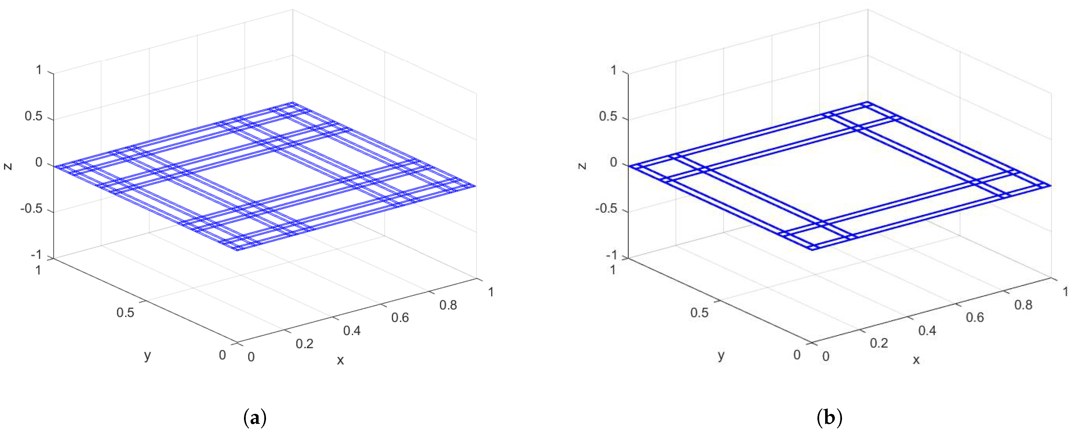
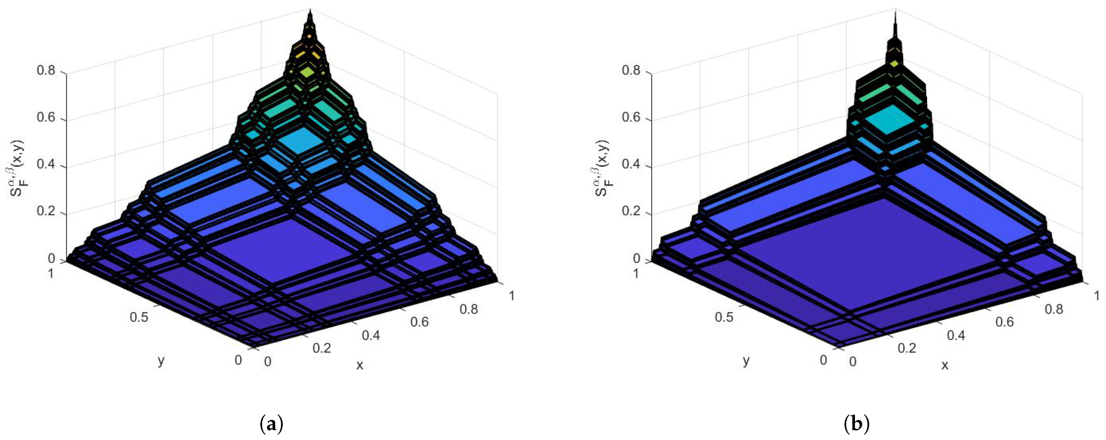
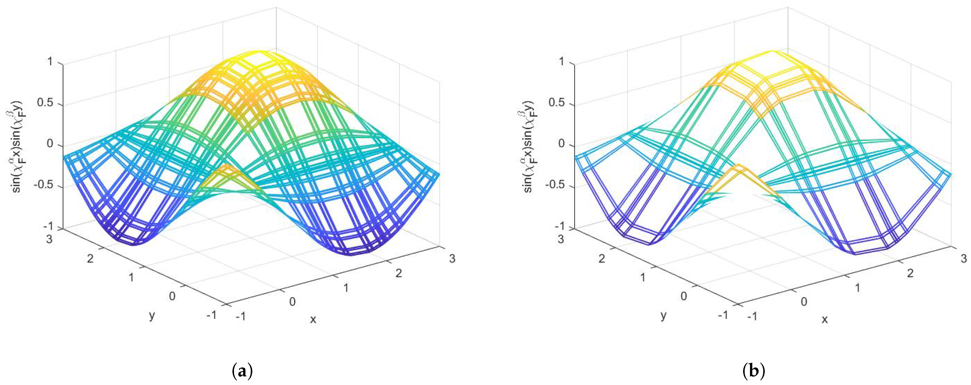
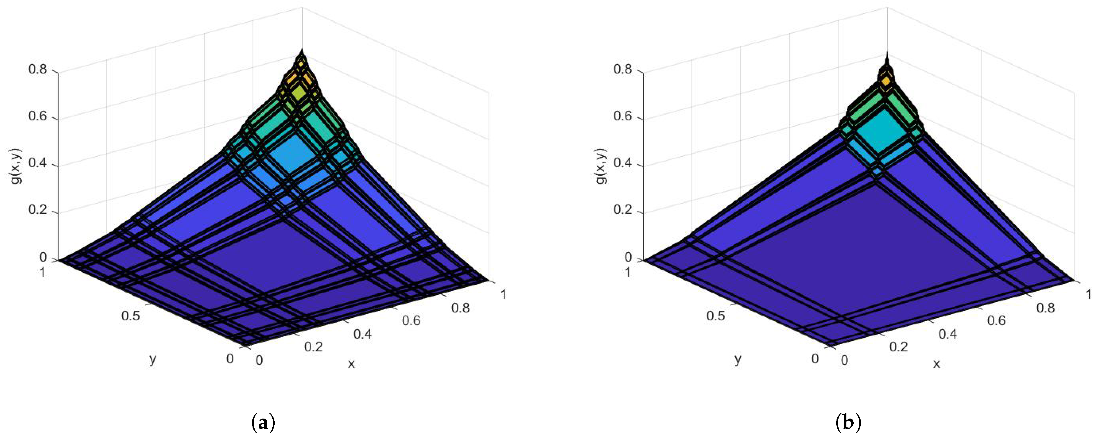
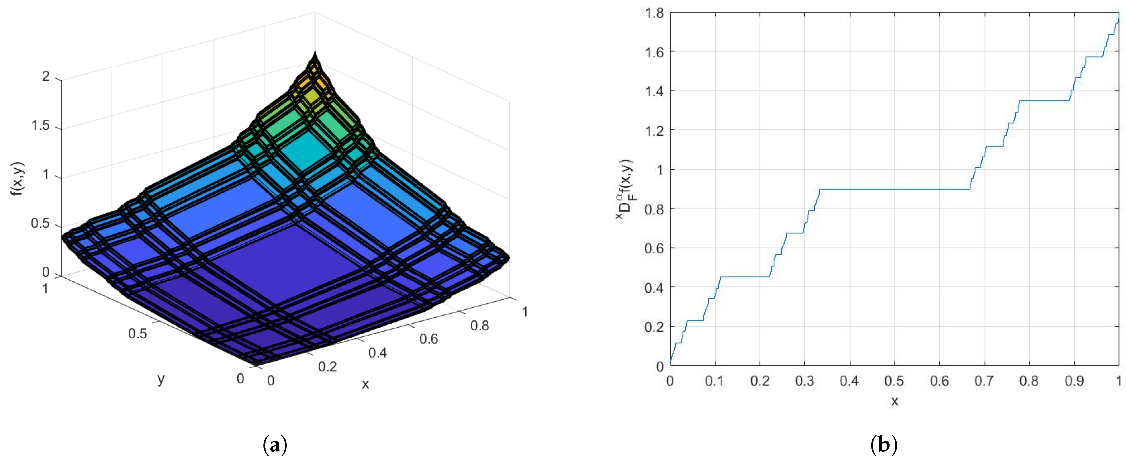
3. Example Functions with Cantor Tartan Support

The task is now to apply definitions to examples. In this section, we give some examples to show more details.

Example 2.

Let us consider the following function, supported on the Cantor tartan with different fractal dimensions:

$$f(x,y)=sin(x{\chi }_F^{\eta }(x))sin(y{\chi }_F^{ϵ}(y)),(x,y)\in \mathbb{F},$$

(19)

where ${\chi }_F^{\eta },{\chi }_F^{ϵ}$ are characteristic functions for the fractal sets $F_1,F_2$ whose union is $\mathbb{F}$ [40,43] (the indices η and ϵ denote the dimension of the respective Cantor sets used to form the sets $F_1$ and $F_2$). Graphs of the function $f(x,y)$ are shown in Figure 3.

The fractal integral of $f(x,y)$ on the Cantor tartan $\mathbb{F}\subset [0,1]\times [0,1]$ is as follows:

$$\begin{array}{cc}g(x,y){|}_{(x=y=1)}\hfill & ={\int }_0^x{\int }_0^{y}sin({\chi }_F^{\eta }x)sin({\chi }_F^{ϵ}y)d_F^{\eta }{x}^{\prime }{d}_F^{ϵ}{y}^{\prime }{|}_{(x=y=1)}\hfill \\ & ={\int }_0^1\Gamma (ϵ+1)cos\left(\frac{S_F^{ϵ}(y^{\prime })}{\Gamma (ϵ+1)}\right)sin({\chi }_F^{\eta }x){|}_0^1{d}_F^{\eta }{x}^{\prime }\hfill \\ & ={\int }_0^1[\Gamma (ϵ+1)cos\left(\frac{S_F^{ϵ}(1)}{\Gamma (ϵ+1)}\right)sin({\chi }_F^{\eta }x)\hfill \\ & -\Gamma (ϵ+1)cos\left(\frac{S_F^{ϵ}(0)}{\Gamma (ϵ+1)}\right)sin({\chi }_F^{\eta }x)]d_F^{\eta }{x}^{\prime }\hfill \\ & =\Gamma (ϵ+1)\Gamma (\eta +1)\left(cos(1)cos\left(\frac{S_F^{ϵ}(x^{\prime })}{\Gamma (\eta +1)}\right)-cos\left(\frac{S_F^{ϵ}(x^{\prime })}{\Gamma (\eta +1)}\right)\right){|}_0^1\hfill \\ & =\Gamma (ϵ+1)\Gamma (\eta +1){(cos(1)-1)}^2\hfill \end{array}$$

(20)

since here $S_F^{\eta }(1)=\Gamma (1+\eta ),S_F^{ϵ}(1)=\Gamma (1+ϵ),S_F^{\eta }(0)=S_F^{ϵ}(0)=0$ [39]. We note the following special cases as examples:

$$g(x,y){|}_{(x=y=1)}=\left\{\begin{array}{cc}0.170,\hfill & \eta =ϵ=0.63(Cantortartanofdimension1.63)\hfill \\ 0.165,\hfill & \eta =ϵ=0.43(Cantortartanofdimension1.43)\hfill \end{array}\right.$$

(21)

In Figure 4, we sketch the function $g(x,y)$, which is called the fractal integral of $f(x,y)$.

Example 3.

Consider a function with Cantor tartan support as follows:

$$f(x,y)=sin(x{\chi }_F^{\eta }(x)+y{\chi }_F^{ϵ}(y)),(x,y)\in \mathbb{F}$$

(22)

We present in Figure 5 the graph of Equation (22). The fractal integral of Equation (22) is as follows:

$$\begin{array}{cc}\hfill g(x,y){|}_{(x=y=1)}& ={\int }_0^x{\int }_0^{y}sin({\chi }_F^{\eta }x+{\chi }_F^{ϵ}y)d_F^{\eta }{x}^{\prime }{d}_F^{ϵ}{y}^{\prime }{|}_{(x=y=1)}\hfill \\ & ={\int }_0^1-\Gamma (ϵ+1)cos\left({\chi }_F^{\eta }x+\frac{S_F^{ϵ}(y)}{\Gamma (ϵ+1)}\right){|}_0^1{d}_F^{\eta }{x}^{\prime }\hfill \\ & ={\int }_0^1[-\Gamma (ϵ+1)cos({\chi }_F^{\eta }x+1)+\Gamma (ϵ+1)cos({\chi }_F^{\eta }x)]d_F^{\eta }{x}^{\prime }\hfill \\ & =-\Gamma (\eta +1)\Gamma (ϵ+1)sin\left(\frac{S_F^{\eta }(x^{\prime })}{\Gamma (\eta +1)}+1\right)\hfill \\ & +\Gamma (\eta +1)\Gamma (ϵ+1)sin\left(\frac{S_F^{\eta }(x^{\prime })}{\Gamma (\eta +1)}\right){|}_0^1\hfill \\ & =\Gamma (\eta +1)\Gamma (ϵ+1)[2sin(1)-sin(2)]\hfill \end{array}$$

(23)

since $S_F^{\eta }(1)=\Gamma (1+\eta ),S_F^{ϵ}(1)=\Gamma (1+ϵ),S_F^{\eta }(0)=S_F^{ϵ}(0)=0$ [39]. We note the following special cases as examples:

$$g(x,y){|}_{(x=y=1)}=\left\{\begin{array}{cc}0.622,\hfill & \eta =ϵ=0.63(Cantortartanofdimension1.63)\hfill \\ 0.607,\hfill & \eta =ϵ=0.43(Cantortartanofdimension1.43)\hfill \end{array}\right.$$

(24)

In Figure 6, we plot the fractal integral of $sin(x{\chi }_F^{\eta }(x)+y{\chi }_F^{ϵ}(y))$ supported on Cantor tartan spaces with different dimensions.

Example 4.

Consider a function on a Cantor tartan space as follows:

$$f(x,y)=S_F^{\eta }{(x)}^2+S_F^{ϵ}{(y)}^2.$$

(25)

The fractal partial derivatives of $f(x,y)$ with respect to x and y are:

$${}^x{D}_F^{\eta }f(x,y)=2S_F^{\eta }(x),{}^y{D}_F^{\eta }f(x,y)=2S_F^{\eta }(y).$$

(26)

In Figure 7, we plot Equation (25) and also its partial derivative ${}^x{D}_F^{\eta }f(x,y)$.

Remark 1.

One can obtain standard results by choosing $\eta =1,$ $ϵ=1$, to get $\mathbb{F}=[0,1]\times [0,1]$, which leads to $S_F^{\eta }(x)=x,S_F^{ϵ}(y)=y$.

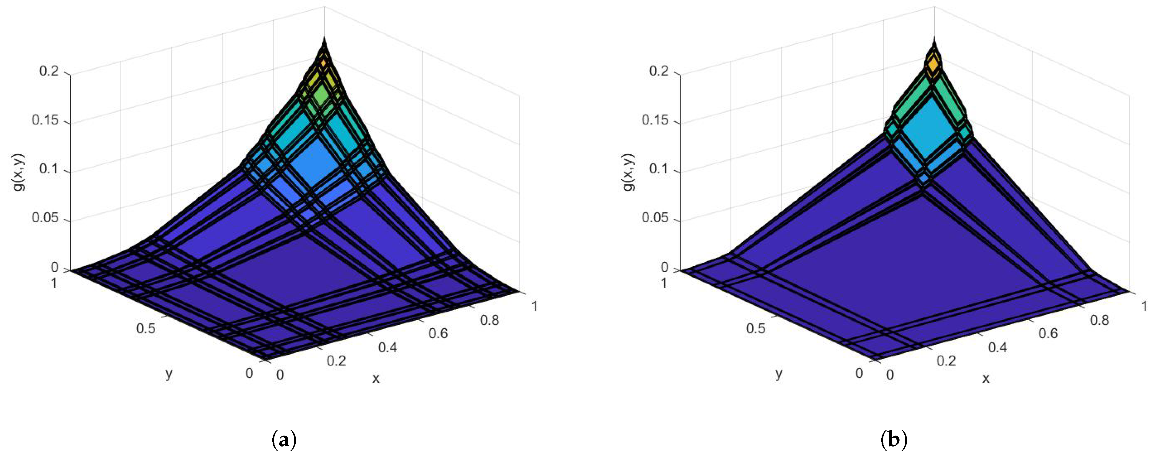
4. Anomalous Diffusion on the Fractal Cantor Tartan

As an example application of the ideas in Section 2, we consider the diffusion equation on the Cantor tartan as the following:

$${}_0^C{\mathcal{D}}_t^{\beta }u(x,y,t)=\mathbf{K}\left({{(}^x{D}_F^{\eta })}^{2}u(x,y,t)+{{(}^y{D}_F^{\eta })}^{2}u(x,y,t)\right),$$

(27)

for $(x,y)\in \mathbb{F}$ and $t\in F$. Here, ${}_0^C{\mathcal{D}}_t^{\beta }$ is the left-sided Caputo-like fractional derivative of order $\beta$ on a fractal set F (see [43]); the fractal derivatives on the right-hand side of (27) are as defined in Section 2; and $\mathbf{K}$ is the diffusion coefficient. We also impose the following initial and boundary conditions:

$$u(x,y,t)=0,(x,y)\in \partial \mathbb{F},t>0,$$

(28)

$$u(x,y,0)=sin(x\pi )sin(y\pi ),(x,y)\in \mathbb{F}\cup \partial \mathbb{F}.$$

(29)

The solution of the differential Equation (27), using the conjugacy of $F^{\eta }$-calculus and standard calculus as described in [39,40], will be [31]:

$$u(x,y,t)=sin(S_F^{\eta }(x)\pi )sin(S_F^{\eta }(y)\pi )E_{F,\beta }^{\eta }\left(-2{(S_F^{\eta }(t))}^{ϵ}\right),\mathbf{K}=\frac{1}{\pi },$$

(30)

where $E_{F,\beta }^{\eta }(.)$ is the generalised Mittag–Leffler function on a Cantor set [43].

If we consider a random walk on a fractal Cantor tartan set, the probability distribution will be described by Equation (27). Thus, the analysis presented here will be useful in modelling different random walks on fractal sets [44,45]. Future research in the field of random walks on fractal sets may be able to proceed along such lines as these.

5. Conclusions

In this work, we define the local derivative and integral on the Cantor tartan. The standard calculus cannot be applied to integrate and differentiate functions on fractals of this form. Therefore, we need a new type of calculus to calculate the physical properties and describe phenomena on fractals. As a result, the $F^{\eta }$-calculus on the Cantor tartan of fractal dimension $1<\zeta <2$ is given. Furthermore, we recall the standard calculus results, which show that the suggested definitions are the natural generalisation of standard calculus. Three illustrative examples were investigated, and the corresponding graphs of the functions were drawn.

References

1. Mandelbrot, B.B. The Fractal Geometry of Nature; W. H. Freeman and Company: New York, NY, USA, 1982. [Google Scholar]
2. Falconer, K. Techniques in Fractal Geometry; John Wiley & Sons: Hoboken, NJ, USA, 1997. [Google Scholar]
3. Cattani, C.; Pierro, G. On the fractal geometry of DNA by the binary image analysis. Bull. Math. Biol. 2013, 75, 1544–1570. [Google Scholar] [CrossRef] [PubMed]
4. Heydari, M.H.; Hooshmandasl, M.R.; Maalek Ghaini, F.M.; Cattani, C. Wavelets method for the time fractional diffusion-wave equation. Phys. Lett. A 2015, 379, 71–76. [Google Scholar] [CrossRef]
5. Freiberg, U.; Zahle, M. Harmonic calculus on fractals-a measure geometric approach I. Potential Anal. 2002, 16, 265–277. [Google Scholar] [CrossRef]
6. Barlow, M.T.; Perkins, E.A. Brownian motion on the Sierpinski gasket, Probab. Theory Relat. Fields 1988, 79, 543–623. [Google Scholar] [CrossRef]
7. Metzler, R.; Klafter, J. Boundary value problems for fractional diffusion equations. Phys. A Stat. Mech. Appl. 2000, 278, 107–125. [Google Scholar] [CrossRef]
8. Agarwal, R.P.; Bohner, M. Basic calculus on time scales and some of its applications. Results Math. 1999, 35, 3–22. [Google Scholar] [CrossRef]
9. Agarwal, R.P.; Mahmoud, R.R.; Saker, S.H.; Tunc, C. New generalizations of Németh–Mohapatra type inequalities on time scales. Acta Math. Hung. 2017, 152, 383–403. [Google Scholar] [CrossRef]
10. Kigami, J. Analysis on Fractals. Volume 143 of Cambridge Tracts in Mathematics; Cambridge University Press: Cambridge, UK, 2001. [Google Scholar]
11. Bohner, M.; Peterson, A. Dynamic Equations on Time Scales: An Introduction with Applications; Birkhäuser: Boston, MA, USA, 2001. [Google Scholar]
12. Naqvi, Q.A.; Fiaz, M.A. Electromagnetic behavior of a planar interface of non-integer dimensional spaces. J. Electromagn. Waves Appl. 2017, 31, 625–1637. [Google Scholar] [CrossRef]
13. Strichartz, R.S. Differential Equations on Fractals: A Tutorial; Princeton University Press: Princeton, NJ, USA, 2006. [Google Scholar]
14. Tarasov, V.E. Fractional Dynamics: Applications of Fractional Calculus to Dynamics of Particles, Fields and Media; Springer: New York, NY, USA, 2011. [Google Scholar]
15. Brossard, J.; Carmona, R. Can one hear the dimension of fractal? Commun. Math. Phys. 1986, 104, 103–122. [Google Scholar] [CrossRef]
16. Tatom, F.B. The relationship between fractional calculus and fractals. Fractals 1995, 3, 217–229. [Google Scholar] [CrossRef]
17. Nigmatullin, R.R.; Zhang, W.; Gubaidullin, I. Accurate relationships between fractals and fractional integrals: New approaches and evaluations. Fract. Calc. Appl. Anal. 2017, 20, 1263–1280. [Google Scholar] [CrossRef] [Green Version]
18. Butera, S.; Paola, M.D. A physically based connection between fractional calculus and fractal geometry. Ann. Phys. 2014, 350, 146–158. [Google Scholar] [CrossRef] [Green Version]
19. Herrmann, R. Fractional Calculus: An Introduction for Physicists; World Scientific: London, UK, 2014. [Google Scholar]
20. Hilfer, R. (Ed.) Applications of Fractional Calculus in Physics; World Scientific: London, UK, 2000. [Google Scholar]
21. Nigmatullin, R.R.; Evdokimov, Y.K. The concept of fractal experiments: New possibilities in quantitative description of quasi-reproducible measurements. Chaos Soliton Fract. 2016, 9, 319–328. [Google Scholar] [CrossRef]
22. Uchaikin, V.V. Fractional Derivatives for Physicists and Engineers Vol. 1 Background and Theory; Application Springer: Berlin, Germany, 2013; Volume 2. [Google Scholar]
23. Wu, G.C.; Baleanu, D.; Xie, H.P.; Chen, F.L. Chaos synchronization of fractional chaotic maps based on stability results. Phys. A Stat. Mech. Appl. 2016, 460, 374–383. [Google Scholar] [CrossRef]
24. Magin, R.L. Fractional Calculus in Bioengineering; Begell House Publisher, Inc.: Connecticut, CT, USA, 2006. [Google Scholar]
25. Malinowska, A.B.; Torres, D.F.M. Introduction to the Fractional Calculus of Variations; Imperial College Press: London, UK, 2012. [Google Scholar]
26. Podlubny, I. Fractional Differential Equations; Academic Press: New York, NY, USA, 1999. [Google Scholar]
27. Chen, W. Time-space fabric underlying anomalous diffusion. Chaos Solitons Fract. 2006, 28, 923–929. [Google Scholar] [CrossRef]
28. Chen, W.; Sun, H.G.; Zhang, X.; Koroak, D. Anomalous diffusion modeling by fractal and fractional derivatives. Comp. Math. Appl. 2010, 59, 1754–1758. [Google Scholar] [CrossRef]
29. Arkhincheev, V.E.; Baskin, E.M. Anomalous diffusion and drift in a comb model of percolation clusters. Sov. Phys. JETP 1991, 73, 161–300. [Google Scholar]
30. Sandev, T.; Iomin, A.; Kantz, H. Fractional diffusion on a fractal grid comb. Phys. Rev. E 2015, 91, 032108. [Google Scholar] [CrossRef] [PubMed]
31. Çetinkaya, A.; Kıymaz, O. The solution of the time-fractional diffusion equation by the generalized differential transform method. Math. Comput. Model. 2013, 57, 2349–2354. [Google Scholar] [CrossRef]
32. Kameke, A.V.; Huhn, F.; Fernández-García, G.; Muñuzuri, V.; Pérez-Muñuzuri, A.P. Propagation of a chemical wave front in a quasi-two-dimensional superdiffusive flow. Phys. Rev. E 2010, 81, 066211. [Google Scholar] [CrossRef] [PubMed]
33. Telcs, A. The Art of Random Walks; Springer: New York, NY, USA, 2006. [Google Scholar]
34. Gianvittorio, J.P.; Rahmat-Samii, Y. Fractal antennas: A novel antenna miniaturization technique and applications. IEEE Antennas Propag. 2002, 44, 20–36. [Google Scholar] [CrossRef]
35. Cohen, N. Fractal Antenna Applications in Wireless Telecommunications. In Proceedings of the Electronics Industries Forum of New England, Boston, MA, USA, 6–8 May 1997. [Google Scholar]
36. Balankin, A.S.; Mena, B.; Susarrey, O.; Samayoa, D. Steady laminar flow of fractal fluids. Phys. Lett. A 2017, 381, 623–628. [Google Scholar] [CrossRef]
37. Butera, S.; Di Paola, M. A physical approach to the connection between fractal geometry and fractional calculus. In Proceedings of the 2014 International Conference on Fractional Differentiation and Its Applications, ICFDA 2014, Catania, Italy, 23–25 June 2014; p. 6967378. [Google Scholar] [CrossRef]
38. Balankin, A.S.; Mena, B.; Patino, J.; Morales, D. Electromagnetic fields in fractal continua. Phys. Lett. A 2013, 377, 783–788. [Google Scholar] [CrossRef]
39. Parvate, A.; Gangal, A.D. Calculus on fractal subsets of real line I: Formulation. Fractals 2009, 17, 53–81. [Google Scholar] [CrossRef]
40. Parvate, A.; Gangal, A.D. Calculus on fractal subsets of real line II: Conjugacy with ordinary calculus. Fractals 2011, 19, 271–290. [Google Scholar] [CrossRef]
41. Seema, S.; Gangal, A.D. Langevin Equation on Fractal Curves. Fractals 2016, 24, 1650028. [Google Scholar]
42. Golmankhaneh, A.K.; Fernandez, A.; Golmankhaneh, A.K.; Baleanu, D. Diffusion on middle-ξ Cantor sets. Entropy 2018, 20, 504. [Google Scholar] [CrossRef]
43. Golmankhaneh, A.K.; Baleanu, D. Non-local Integrals and Derivatives on Fractal Sets with Applications. Open Phys. 2016, 14, 542–548. [Google Scholar] [CrossRef] [Green Version]
44. Golmankhaneh, A.K.; Balankin, A.S. Sub-and super-diffusion on Cantor sets: Beyond the paradox. Phys. Lett. A 2018, 382, 960–967. [Google Scholar] [CrossRef]
45. Balankina, A.S.; Golmankhaneh, A.K.; Patiño-Ortiza, J.; Patiño-Ortiz, M. Noteworthy fractal features and transport properties of Cantor tartans. Phys. Lett. A 2018, 382, 1534–1539. [Google Scholar] [CrossRef]
Figure 1. Variants of the Cantor tartan with different dimensions are plotted. (a) Cantor tartan with dimension 1.63; (b) Cantor tartan with dimension 1.43.
Fractalfract 02 00030 g001
Figure 2. The staircase functions corresponding to the Cantor tartan with different dimensions are presented. (a) For the Cantor tartan with dimension 1.63; (b) for the Cantor tartan with dimension 1.43.
Fractalfract 02 00030 g002
Figure 3. We plot the graph of the function sin ( χ F η x ) sin ( χ F ϵ y ) with different Cantor tartan supports. (a) On the Cantor tartan with dimension 1.63; (b) on the Cantor tartan with dimension 1.43.
Fractalfract 02 00030 g003
Figure 4. The fractal integral of sin ( x χ F η ( x ) ) sin ( y χ F ϵ ( y ) ) on the Cantor tartan of different dimensions is sketched. (a) On the Cantor tartan with dimension 1.63; (b) on the Cantor tartan with dimension 1.43.
Fractalfract 02 00030 g004
Figure 5. We plot the graph of the function sin ( x χ F η ( x ) + y χ F ϵ ( y ) ) with different Cantor tartan supports. (a) On the Cantor tartan with dimension 1.63; (b) on the Cantor tartan with dimension 1.43.
Fractalfract 02 00030 g005
Figure 6. The fractal integral of sin ( χ F η x + χ F ϵ y ) on the Cantor tartan of different dimensions is shown. (a) On the Cantor tartan with dimension 1.63; (b) on the Cantor tartan with dimension 1.43.
Fractalfract 02 00030 g006
Figure 7. Graphs of the function S F η ( x ) 2 + S F ϵ ( y ) 2 and its derivative x D F η f ( x , y ) on the Cantor tartan with dimension 1.63. (a) Graph of the function; (b) graph of the derivative.
Fractalfract 02 00030 g007