Minkowski Dimension and Explicit Tube Formulas for p-Adic Fractal Strings


Abstract
Nature is an infinite sphere of which the center is everywhere and the circumference nowhere.Blaise Pascal (1623–1662)
1. Introduction
The inverse spectral problem for a fractal string can be solved if and only if its dimension is not .
2. Nonarchimedean Fractal Strings
2.1. p-Adic Numbers
- (a)
- The distance defined on by is called an ultrametric, since it satisfies the counterpart of the above strong triangle inequality:for all . Consequently, every triangle in is isosceles with the two longer sides having the same length:It follows that the center can be chosen anywhere within the p-adic ball B. Moreover, given any two balls and , either they are disjoint or one is entirely contained in the other (i.e., or ). These special properties are common to all ultrametric spaces (i.e., all metric spaces for which the ultrametric triangle inequality (2) holds).
- (b)
- By definition, is the (closed) unit ball of (). Moreover, has the remarkable property of being a ring (since for all in , by (2) again, , and ). This is to be contrasted with the fact that , the unit ball of , is not stable under addition (although it is obviously stable under multiplication); see [61]. Finally, since translations are homeomorphisms, every closed ball in with center a has a radius r of the form ,for some , the valuation group of the nonarchimedean field . We leave it to the reader to investigate the converse statement according to which every convex subset of is a metric ball (i.e., an interval); see, e.g., [59].
- (c)
- (p-adic intervals). In the sequel (as well as in part of the literature on p-adic analysis, see, e.g., [55]), the metric balls (with and , as in (4) just above), are sometimes called the ‘intervals’ of . Note that they are not connected, in the usual topological sense, but that they are ‘convex’, in the following sense: for each and , we have that . (Here and henceforth, it is useful to think of as being the analogue of the unit interval , rather than of .)
- (d)
- (The archimedean/nonarchimedean dichotomy). A beautiful and classical theorem of Alexander Ostrowski states that each nontrivial absolute value on the field of rational numbers , is either equivalent to the standard archimedean absolute value on or to the nonarchimedean p-adic absolute value for some prime p. (Recall that two absolute values are said to be equivalent if they induce the same topology on ; this is the case if and only if one is a power of the other.) Therefore, infinitely many completions of (one for each prime p) are nonarchimedean and is the only completion of that is archimedean. For this reason, one sometimes writes and refers to (the equivalence class of) the absolute value as the ‘place at infinity’, associated with the ‘prime at infinity’ or the ‘real prime’; see [61]. (We note that Ostrowski’s Theorem is usually expressed in terms of valuations rather than of absolute values. Accordingly, a place of is generally defined as an equivalence class of valuations on .) With this notation in mind, we see that the field is archimedean, whereas for any (finite) prime p, is a nonarchimedean field. The theory of p-adic fractal strings developed in [30,31,32,33] is aimed, initially, at finding suitable definitions and obtaining results that parallel those corresponding to the theory of real (or archimedean) fractal strings developed in [7], for example. As we will see, however, although there are many analogies between the archimedean and nonarchimedean theories of fractal strings, there are also some notable differences between them; see, especially, [32], along with [30,33].
2.2. p-Adic Fractal Strings
2.3. Example: p-Adic Euler String
3. The Geometric Zeta Function
Languid and Strongly Languid p-Adic Fractal Strings
- For all and all
- For all
- There exist constants such that for all and ,
- (a)
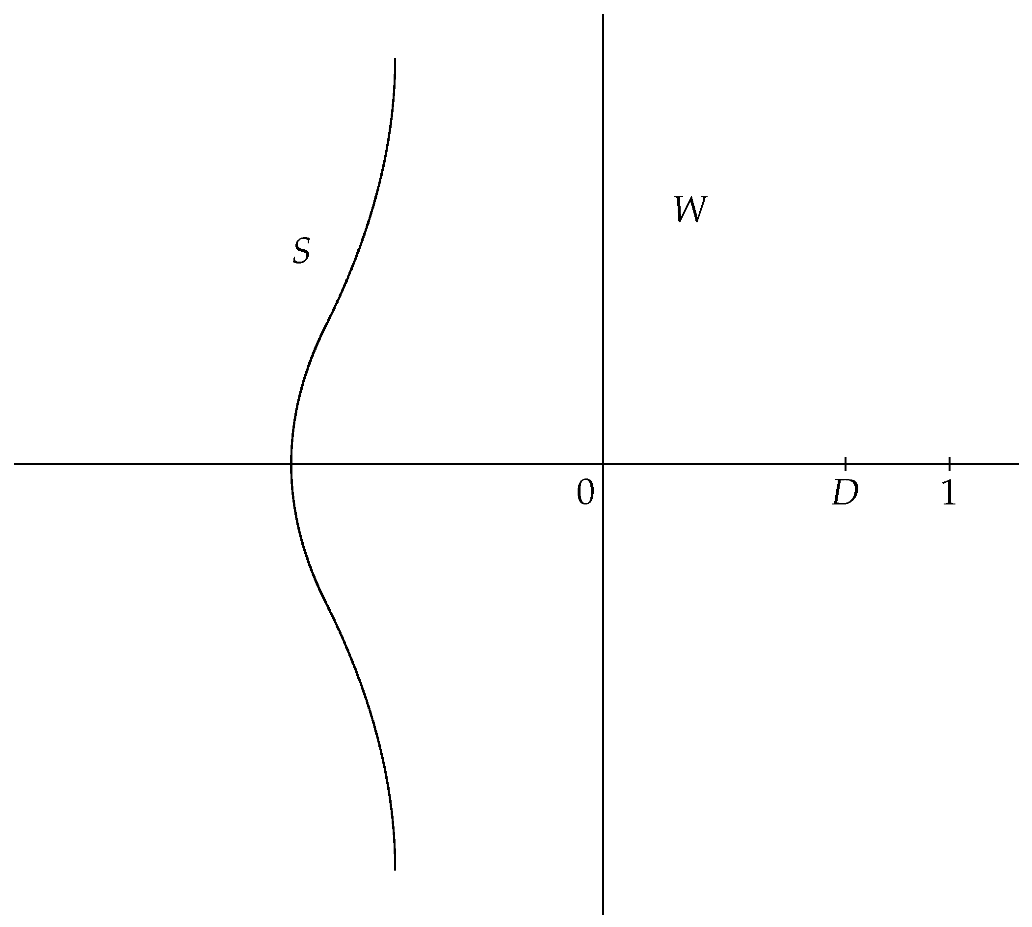
- Intuitively, hypothesis is a polynomial growth condition along horizontal lines (necessarily avoiding the poles of ), while hypothesis is a polynomial growth condition along the vertical direction of the screen.
- (b)
- Clearly, condition is stronger than . Indeed, if is strongly languid, then it is also languid (for each screen separately).
- (c)
- Moreover, if is languid for some κ, then it is also languid for every larger value of κ. The same is also true for strongly languid strings.
- (d)
- Finally, hypotheses and require that has an analytic (i.e., meromorphic) continuation to an open, connected neighborhood of , while requires that has a meromorphic continuation to all of .
4. Volume of Thin Inner Tubes
4.1. Example: The Euler String
5. Minkowski Dimension
5.1. The Real Case
6. Explicit Tube Formulas for -adic Fractal Strings
- (i)
- Let be a languid p-adic fractal string (as in the first part of Definition 5 of Section 3), for some real exponent κ and a screen S that lies strictly to the left of the vertical line . Further assume that (Recall from Corollary 2 that we always have . Moreover, if is self-similar, then Then the volume of the thin inner ε-neighborhood of is given by the following distributional explicit formula, on test functions in , the space of functions with compact support inwhere is the set of visible complex dimensions of (as given in Definition 4 Here, the distributional error term is given byand is estimated distributionally (in the sense of [7], Definition 5.29) by
- (ii)
- Moreover, if is strongly languid (as in the second part of Definition 5), then we can take and , provided we apply this formula to test functions supported on compact subsets of . The resulting explicit formula without error term is often called an exact tube formula in this case.
- (i)
- Because on each relevant vertical line, the complex dimensions form an arithmetic progression (with a progression or period independent of the line) and have the same multiplicities, the corresponding term in the associated fractal tube formula can be written as a suitable power function times a periodic function (of ). (This is so assuming that the complex dimensions on that line are simple, which is always the case, for instance, of the right most vertical line ).
- (ii)
- In all of the concrete examples of p-adic self-similar strings studied in [32,33], including the 3-adic Cantor string and the 2-adic Fibonacci string, the corresponding exact fractal tube formula can be shown to converge pointwise (rather than distributionally, as in Theorem 5). We conjecture that at least in the case of simple complex dimensions, the exact fractal tube formula of a p-adic self-similar string always converges pointwise (and not just distributionally, as in Theorem 5). (Such a result is established in [7], Section 8.4 for general real or archimedean self-similar strings, whether or not all of the complex dimensions are simple.) Accordingly, it would be very interesting to establish that conjecture as well as to obtain a pointwise counterpart of Theorem 5; that is, a fractal tube formula for p-adic (not necessarily self-similar) fractal strings, with or without an error term, which (under suitable hypotheses) would be valid pointwise. We note that in the archimedean case (i.e., for real fractal strings) such a pointwise fractal tube formula is available under rather general conditions; see [7], Section 8.1.1, esp., Theorem 8.7 and Corollary 8.10. We leave the investigation of these issues to some future work or to the interested reader.
7. Possible Extensions
7.1. Adèlic Fractal Strings and Their Spectra
7.2. Nonarchimedean Fractal Strings in Berkovich Space
7.3. Higher-Dimensional Fractal Tube Formulas
8. Epilogue
Author Contributions
Funding
Acknowledgments
Conflicts of Interest
References
- Lapidus, M.L. Fractal drum, inverse spectral problems for elliptic operators and a partial resolution of the Weyl–Berry conjecture. Trans. Am. Math. Soc. 1991, 325, 465–529. [Google Scholar] [CrossRef]
- Lapidus, M.L. Spectral and fractal geometry: From the Weyl–Berry conjecture for the vibrations of fractal drums to the Riemann zeta-function. In Differential Equations and Mathematical Physics, Proceedings of the Fourth UAB International Conference, Birmingham, UK, March 1990; Bennewitz, C., Ed.; Academic Press: New York, NY, USA, 1992; pp. 151–182. [Google Scholar]
- Lapidus, M.L. Vibrations of fractal drums, the Riemann hypothesis, waves in fractal media, and the Weyl–Berry conjecture. In Ordinary and Partial Differential Equations, Vol. IV, Proceedings of the Twelfth International Conference, Dundee, Scotland, UK, June 1992; Sleeman, B.D., Jarvis, R.J., Eds.; Pitman Research Notes in Mathematics Series 289; Longman Scientific and Technical: London, UK, 1993; pp. 126–209. [Google Scholar]
- Lapidus, M.L.; Pomerance, C. The Riemann zeta-function and the one-dimensional Weyl–Berry conjecture for fractal drums. Proc. Lond. Math. Soc. 1993, 66, 41–69. [Google Scholar] [CrossRef]
- Lapidus, M.L.; Maier, H. The Riemann hypothesis and inverse spectral problems for fractal strings. J. Lond. Math. Soc. 1995, 52, 15–34. [Google Scholar] [CrossRef]
- Lapidus, M.L.; van Frankenhuijsen, M. Fractal Geometry and Number Theory: Complex Dimensions of Fractal Strings and Zeros of Zeta Functions; Birkhäuser: Boston, MA, USA, 2000. [Google Scholar]
- Lapidus, M.L.; van Frankenhuijsen, M. Fractal Geometry, Complex Dimensions and Zeta Functions: Geometry and Spectra of Fractal Strings, 2nd Revised and Enlarged Edition of the 2006 Edition; Springer Monographs in Mathematics; Springer: New York, NY, USA, 2013. [Google Scholar]
- Lapidus, M.L. In Search of the Riemann Zeros: Strings, Fractal Membranes and Noncommutative Spacetimes; American Mathematical Society: Providence, RI, USA, 2008. [Google Scholar]
- Herichi, H.; Lapidus, M.L. Quantized Number Theory, Fractal Strings, and the Riemann Hypothesis: From Spectral Operators to Phase Transitions and Universality; Research Monograph; World Scientific Publishing: Singapore; London, UK, 2019; in press; 400p. [Google Scholar]
- Herichi, H.; Lapidus, M.L. Riemann zeros and phase transitions via the spectral operator on fractal strings. J. Phys. A Math. Theor. 2012, 45, 374005. [Google Scholar] [CrossRef]
- Herichi, H.; Lapidus, M.L. Fractal complex dimensions, Riemann hypothesis and invertibility of the spectral operator. In Fractal Geometry and Dynamical Systems in Pure and Applied Mathematics I: Fractals in Pure Mathematics; Carfi, D., Lapidus, M.L., Pearse, E.P.J., van Frankenhuijsen, M., Eds.; Contemporary Mathematics; American Mathematical Society: Providence, RI, USA, 2013; Volume 600, pp. 51–89. [Google Scholar]
- Lapidus, M.L. Towards quantized number theory: Spectral operators and an asymmetric criterion for the Riemann hypothesis. Philos. Trans. R. Soc. Ser. A 2015, 373. [Google Scholar] [CrossRef] [PubMed]
- Lapidus, M.L. The sound of fractals strings and the Riemann hypothesis. In Analytic Number Theory: In Honor of Helmut Maier’s 60th Birthday; Pomerance, C.B., Rassias, T., Eds.; Springer International Publisher: Cham, Switzerland, 2016; pp. 201–252. [Google Scholar]
- Dragovich, B. Adelic harmonic oscillator. Int. J. Mod. Phys. A 1995, 10, 2349–2365. [Google Scholar] [CrossRef]
- Rammal, R.; Toulouse, G.; Virasoro, M.A. Ultrametricity for physicists. Rev. Mod. Phys. 1986, 58, 765–788. [Google Scholar] [CrossRef]
- Vladimirov, V.S.; Volovich, I.V.; Zelenov, E.I. p-adic Analysis and Mathematical Physics; World Scientific Publishing: Singapore, 1994. [Google Scholar]
- Dragovich, B.; Yu, A.; Khrennikov, S.; Kozyrev, S.V.; Volovich, I.V. On p-adic mathematical physics. p-Adic Numbers Ultrametric Anal. Appl. 2009, 1, 1–17. [Google Scholar] [CrossRef]
- Everett, C.J.; Ulam, S. On some possibilities of generalizing the Lorentz group in the special relativity theory. J. Comb. Theory 1966, 1, 248–270. [Google Scholar] [CrossRef]
- Berkovich, V.G. p-adic analytic spaces. In Proceedings of the International Congress of Mathematicians, Berlin, Germany, 18–27 August 1998; Fisher, G., Rehmann, U., Eds.; Documenta Mathematica (Extra Volume ICM 1998). Volume II, pp. 141–151. [Google Scholar]
- Bendikov, A. Heat kernels for isotropic-like Markov generators on ultrametric spaces: A survey. p-Adic Numbers Ultrametric Anal. Appl. 2018, 10, 1–11. [Google Scholar] [CrossRef]
- Bendikov, A.; Grigor’yan, A.; Pittet, C.; Woess, W. Isotropic Markov semigroups on ultrametric spaces. Russ. Math. Surv. 2014, 69, 589–680. [Google Scholar] [CrossRef]
- Pearson, J.; Bellissard, J. Noncommutative Riemannian geometry and diffusion on ultrametric Cantor sets. J. Noncommut. Geom. 2009, 3, 447–480. [Google Scholar] [CrossRef]
- Ducros, A. Espaces analytiques p-adiques au sens de Berkovich. Sémin. Bourbaki 2006, 48, 137–176. [Google Scholar]
- Volovich, I.V. Number Theory as the Ultimate Physical Theory. CERN-TH.4781/87. Available online: http://cds.cern.ch/record/179558/files/198708102.pdf (accessed on 26 September 2018).
- Gibbons, G.W.; Hawking, S.W. (Eds.) Euclidean Quantum Gravity; World Scientific Publishing: Singapore, 1993. [Google Scholar]
- Hawking, S.W.; Israel, W. (Eds.) General Relativity: An Einstein Centenary Survey; Cambridge University Press: Cambridge, UK, 1979. [Google Scholar]
- Notale, L. Fractal Spacetime and Microphysics: Towards a Theory of Scale Relativity; World Scientific Publishing: Singapore, 1993. [Google Scholar]
- Wheeler, J.A.; Ford, K.W. Geons, Black Holes, and Quantum Foam: A Life in Physics; Norton, W.W.: New York, NY, USA, 1998. [Google Scholar]
- Lapidus, M.L.; Nest, R. Fractal membranes as the second quantization of fractal strings. 2018; in preparation. [Google Scholar]
- Lapidus, M.L.; Lũ’, H. Nonarchimedean Cantor set and string. J. Fixed Point Theory Appl. 2008, 3, 181–190. [Google Scholar] [CrossRef]
- Lapidus, M.L.; Lũ’, H. Self-similar p-adic fractal strings and their complex dimensions. p-Adic Numbers Ultrametric Anal. Appl. 2009, 1, 167–180. [Google Scholar] [CrossRef]
- Lapidus, M.L.; Lũ’, H. The geometry of p-adic fractal strings: A comparative survey. In Advances in Non-Archimedean Analysis, Proceedings of the 11th International Conference on “p-Adic Functional Analysis”, Clermont-Ferrand, France, 5–9 July 2010; Araujo, J., Diarra, B., Escassut, A., Eds.; Contemporary Mathematics; American Mathematical Society: Providence, RI, USA, 2011; Volume 551, pp. 163–206. [Google Scholar]
- Lapidus, M.L.; Lũ’, H.; van Frankenhuijsen, M. Minkowski measurability and exact fractal tube formulas for p-adic self-similar strings. In Fractal Geometry and Dynamical Systems in Pure Mathematics. I: Fractals in Pure Mathematics; Carfí, D., Lapidus, M.L., Pearse, E.P.J., van Frankenhuijsen, M., Eds.; Contemporary Mathematics; American Mathematical Society: Providence, RI, USA, 2013; Volume 600, pp. 161–184. [Google Scholar]
- Lapidus, M.L.; Radunović, G.; Žubrinić, D. Fractal Zeta Functions and Fractal Drums: Higher-Dimensional Theory of Complex Dimensions; Springer Monographs in Mathematics; Springer: New York, NY, USA, 2017. [Google Scholar]
- Ellis, K.E.; Lapidus, M.L.; Mackenzie, M.C.; Rock, J.A. Partition zeta functions, multifractal spectra, and tapestries of complex dimensions. In Benoit Mandelbrot: A Life in Many Dimensions; Frame, M., Cohen, N., Eds.; The Mandelbrot Memorial Volume; World Scientific: Singapore, 2015; pp. 267–312. [Google Scholar]
- Falconer, K.J. On the Minkowski measurability of fractals. Proc. Am. Math. Soc. 1995, 123, 1115–1124. [Google Scholar] [CrossRef]
- Hambly, B.M.; Lapidus, M.L. Random fractal strings: Their zeta functions, complex dimensions and spectral asymptotics. Trans. Am. Math. Soc. 2006, 358, 285–314. [Google Scholar] [CrossRef]
- He, C.Q.; Lapidus, M.L. Generalized Minkowski content, spectrum of fractal drums, fractal strings and the Riemann zeta-function. Mem. Am. Math. Soc. 1997, 127, 1–97. [Google Scholar] [CrossRef]
- Kombrink, S. A survey on Minkowski measurability of self-similar sets and self-conformal fractals in , survey article. In Fractal Geometry and Dynamical Systems in Pure and Applied Mathematics I: Fractals in Pure Mathematics; Carfi, D., Lapidus, M.L., Pearse, E.P.J., van Frankenhuijsen, M., Eds.; Contemporary Mathematics; American Mathematical Society: Providence, RI, USA, 2013; Volume 600, pp. 135–159. [Google Scholar]
- Lapidus, M.L.; Pearse, E.P.J. Tube formulas for self-similar fractals. In Analysis on Graphs and Its Applications; Exner, P., Keating, J.P., Kuchment, P., Teplyaev, A., Sunada, T., Eds.; Proceedings of Symposia in Pure Mathematics Volume 77; American Mathematical Society: Providence, RI, USA, 2008; pp. 211–230. [Google Scholar]
- Lapidus, M.L.; Pearse, E.P.J. Tube formulas and complex dimensions of self-similar tilings. Acta Math. Appl. 2010, 112, 91–137. [Google Scholar] [CrossRef]
- Lapidus, M.L.; Pearse, E.P.J.; Winter, S. Pointwise tube formulas for fractal sprays and self-similar tilings with arbitrary generators. Adv. Math. 2011, 227, 1349–1398. [Google Scholar] [CrossRef]
- Lapidus, M.L.; Pomerance, C. Counterexamples to the modified Weyl–Berry conjecture for fractal drums. Math. Proc. Camb. Philos. Soc. 1996, 119, 167–178. [Google Scholar] [CrossRef]
- Lapidus, M.L.; Lévy Véhel, J.; Rock, J.A. Fractal strings and multifractal zeta functions. Lett. Math. Phys. 2009, 88, 101–129. [Google Scholar] [CrossRef]
- Lapidus, M.L.; Radunović, G.; Žubrinić, D. Zeta functions and complex dimensions of relative fractal drums: Theory, examples and applications. Diss. Math. 2017, 526, 1–105. [Google Scholar] [CrossRef]
- Lapidus, M.L.; Radunović, G.; Žubrinić, D. Fractal tube formulas and a Minkowski measurability criterion for compact subsets of Euclidean spaces. Discret. Contin. Dyn. Syst. Ser. S 2019, 12, 105–117. [Google Scholar] [CrossRef]
- Lapidus, M.L.; Radunović, G.; Žubrinić, D. Fractal tube formulas for compact sets and relative fractal drums: Oscillations, complex dimensions and fractality. J. Fractal Geom. 2018, 5, 1–119. [Google Scholar] [CrossRef]
- Lapidus, M.L.; Radunović, G.; Žubrinić, D. Minkowski measurability criteria for compact sets and relative fractal drums in Euclidean spaces. arXiv, 2016; arXiv:160904498v1. [Google Scholar]
- Lapidus, M.L.; Radunović, G.; Žubrinić, D. Fractal zeta functions and complex dimensions of relative fractal drums. J. Fixed Point Theory Appl. 2014, 15, 321–378. [Google Scholar] [CrossRef]
- Lapidus, M.L.; Rock, J.A. Towards zeta functions and complex dimensions of multifractals. Complex Var. Elliptic Equ. 2009, 54, 545–560. [Google Scholar] [CrossRef]
- Mora, G.; Sepulcre, J.M.; Vidal, T. On the existence of exponential polynomials with prefixed gaps. Bull. Lond. Math. Soc. 2013, 45, 1148–1162. [Google Scholar] [CrossRef]
- Olsen, L. Multifractal tubes: Multifractal zeta functions, multifractal Steiner tube formulas and explicit formulas. In Fractal Geometry and Dynamical Systems in Pure and Applied Mathematics I: Fractals in Pure Mathematics; Carfi, D., Lapidus, M.L., van Frankenhuijsen, M., Eds.; Contemporary Mathematics; American Mathematical Society: Providence, RI, USA, 2013; Volume 600, pp. 291–326. [Google Scholar]
- Pearse, E.P.J. Canonical self-affine tilings by iterated function systems. Indiana Univ. Math. J. 2007, 56, 3151–3169. [Google Scholar] [CrossRef]
- Lapidus, M.L. An overview of complex fractal dimensions: From fractal strings to fractal drums, and back. In Horizons of Fractal Geometry and Complex Dimensions; Niemeyer, R.G., Pearse, E.P.J., Rock, J.A., Samuel, T., Eds.; American Mathematical Society: Providence, RI, USA, 2019; in press. [Google Scholar]
- Koblitz, N. p-Adic Numbers, p-Adic Analysis, and Zeta-Functions; Springer: New York, NY, USA, 1984. [Google Scholar]
- Neukirch, J. Algebraic Number Theory; A Series of Comprehensive Studies in Mathematics; Springer: New York, NY, USA, 1999. [Google Scholar]
- Manin, Y.I.; Panchishkin, A.A. Number Theory, Vol. I, Introduction to Number Theory; Parshin, A.N., Shafarevich, I.R., Eds.; Encyclopedia of Mathematical Sciences; Springer: Berlin, Germany, 1995; Volume 49. [Google Scholar]
- Robert, A.M. A Course in p-Adic Analysis; Graduate Texts in Mathematics; Springer: New York, NY, USA, 2000. [Google Scholar]
- Schikhof, W.H. Ultrametric Calculus: An Introduction to p-Adic Analysis; Cambridge Studies in Advanced Mathematics; Cambridge University Press: Cambridge, UK, 1984. [Google Scholar]
- Serre, J.-P. A Course in Arithmetic; English Translation; Springer: Berlin, Germany, 1973. [Google Scholar]
- Haran, M.J.S. The Mysteries of the Real Prime; London Mathematical Society Monographs Series; Oxford University Press: Oxford, UK, 2001. [Google Scholar]
- Riemann, B. Ueber die Anzahl der Primzahlen unter einer gegebenen Grösse. Monatsber. Berl. Akad. 1858, 671–680. [Google Scholar]
- Edwards, H.M. Riemann’s Zeta Function; Academic Press: New York, NY, USA, 1974. [Google Scholar]
- Böttcher, A.; Silbermann, B. Analysis of Toeplitz Operators, 2nd ed.; Springer Monographs in Mathematics; Springer: New York, NY, USA, 2006. [Google Scholar]
- Connes, A. Noncommutative Geometry; Academic Press: New York, NY, USA, 1994. [Google Scholar]
- Grebogi, C.; McDonald, S.; Ott, E.; York, J. Exterior dimension of fat fractals. Phys. Lett. A 1985, 110, 1–4. [Google Scholar] [CrossRef]
- Ott, E. Fat Fractals. In Chaos in Dynamical Systems; Cambridge University Press: New York, NY, USA, 1993; Section 3.9; pp. 97–100. [Google Scholar]
- Besicovitch, A.S.; Taylor, S.J. On the complementary intervals of a linear closed set of zero Lebesgue measure. J. Lond. Math. Soc. 1954, 29, 449–459. [Google Scholar] [CrossRef]
- Hutchinson, J.E. Fractals and self-similarity. Indiana Univ. Math. J. 1981, 30, 713–747. [Google Scholar] [CrossRef]
- Falconer, K.J. Fractal Geometry: Mathematical Foundations and Applications, 3rd ed.; Wiley: Chichester, UK, 2014. [Google Scholar]
- Kumar, A.; Rani, M.; Chugh, R. New 5-adic Cantor sets and fractal string. SpringerPlus 2013, 2, 654. [Google Scholar] [CrossRef] [PubMed]

© 2018 by the authors. Licensee MDPI, Basel, Switzerland. This article is an open access article distributed under the terms and conditions of the Creative Commons Attribution (CC BY) license (http://creativecommons.org/licenses/by/4.0/).
Share and Cite
Lapidus, M.L.; Lũ’, H.; Van Frankenhuijsen, M. Minkowski Dimension and Explicit Tube Formulas for p-Adic Fractal Strings. Fractal Fract. 2018, 2, 26. https://doi.org/10.3390/fractalfract2040026
Lapidus ML, Lũ’ H, Van Frankenhuijsen M. Minkowski Dimension and Explicit Tube Formulas for p-Adic Fractal Strings. Fractal and Fractional. 2018; 2(4):26. https://doi.org/10.3390/fractalfract2040026
Chicago/Turabian StyleLapidus, Michel L., Hùng Lũ’, and Machiel Van Frankenhuijsen. 2018. "Minkowski Dimension and Explicit Tube Formulas for p-Adic Fractal Strings" Fractal and Fractional 2, no. 4: 26. https://doi.org/10.3390/fractalfract2040026
APA StyleLapidus, M. L., Lũ’, H., & Van Frankenhuijsen, M. (2018). Minkowski Dimension and Explicit Tube Formulas for p-Adic Fractal Strings. Fractal and Fractional, 2(4), 26. https://doi.org/10.3390/fractalfract2040026