1. Introduction
Fractional calculus (FC) can be traced back to the 17th century when mathematicians like Leibniz and Euler studied the idea of generalizing the derivative and integral orders. Nevertheless, it was in the 19th century when FC was formally established, owing to the efforts of mathematicians like Liouville and Riemann [
1,
2,
3]. In recent years, FC has gained significant attention because of its potential to model complex systems that display long-range memory effects and anomalous diffusion, as observed in different scientific and technological fields [
4]. This mathematical tool has been utilized by researchers to describe complex behaviors that cannot be adequately handled by the usual integer-order integration and differentiation operators, as discussed in [
5,
6,
7] and the references within. When simulating intricate natural phenomena, FC overcomes the drawbacks of conventional integrals and derivatives [
8,
9]. According to sources [
3,
10,
11], this mathematical framework has been successful in analyzing a variety of situations across multiple domains by using fractional operators. Recently, Fractional Differential Equations (FDEqs) have attracted considerable attention from various researchers due to their increased potential for modeling real-life situations accurately in various domains of engineering and scientific applications [
12,
13,
14]. Consequently, considerable research has been undertaken to develop effective mathematical theories and analytical approaches for solving FDEs [
15,
16,
17,
18,
19]. These studies aim to improve the understanding of the dynamics of FDEs and provide accurate predictions of their behavior [
20,
21,
22,
23,
24]. Related developments have further contributed to the analysis and solution of fractional models [
25]. To tackle the challenges associated with FDEqs, various approaches have been proposed to approximate the solutions for FDEqs and their systems [
26,
27]. Among the notable approaches are the modified Adomian decomposition method (ADM) [
28], the fractional variational-iteration method (FVIM) [
29,
30], and the homotopy perturbation method (HPM) [
31,
32,
33]. In addition to this, RPST improves the solution of FDEqs incrementally by representing the residual error in power series form. Initially presented in [
16], Arqub successfully used RPST to solve fuzzy first-order and second-order DEqs by solving linear equations with one or two variables.
In the years since, the core methodology has experienced crucial algorithmic evolution, focusing extensively on pairing residual computations with custom integral transforms to resolve multidimensional non-linear operator maps [
34] as well as adapting power series solutions to generalized
-Caputo formulations without reliance on low-order reductions [
35].
RPST stands out for several reasons [
19]. Firstly, it does not require coefficient comparison and recursion relations; hence, it is easy to implement. Secondly, it guarantees the convergence of the series by effectively minimizing the residual errors. Thirdly, the methodology is robust to computational rounding errors; hence, it requires minimal memory and computational time. Finally, it elegantly handles the transitions between different orders and nonlinearities; hence, it can be readily applied to problems where a reasonable guess is available. In conclusion, the above methodologies, among other approaches, are useful tools for approximating the solutions to FDEqs and have been successfully implemented for a wide range of linear and nonlinear problems.
The convection–diffusion equation is a useful approach for describing the combined effect of convection and diffusion on the movement of various substances or their properties in a medium. This approach is widely used in many fields related to mass transfer, heat transfer, fluid dynamics, etc. One such scenario that we can relate is that of a river’s flow, where the speed of the water helps in transporting substances such as salt. The general formulation of time-fractional convection–diffusion equations (TFC-DEqs) is given by
where
denotes the variable of interest,
symbolizes the diffusion coefficient (which may refer to mass or thermal diffusion),
represents the average velocity of the substance in question,
serves as the source term for
, and ∇ indicates the gradient operator.
Before proceeding, it is essential to address the dimensional homogeneity of the fractional governing equations. Due to the nature of the Caputo fractional derivative, the operator carries fractional physical dimensions of . To ensure the equations are dimensionally consistent across the entire interval , we present the governing equations in a non-dimensionalized form.
Let
and
be the characteristic time and length scales, respectively. We introduce the following dimensionless variables
where
is the characteristic velocity. Substituting these into the dimensional equations and dropping the asterisks for simplicity, we obtain the dimensionless forms presented in Equations (1) and (7). In this dimensionless framework, the fractional operators and all transport coefficients are treated as dimensionless quantities.
The Caputo sense is employed for defining the fractional derivative in the context of this equation. Extensive research has been conducted on this equation in classical contexts, utilizing a variety of analytical and numerical techniques. Notable methods include the VIM [
36], HPM [
37], and the Laplace transform HPM [
38]. Within the domain of FC, ADM has also been applied [
39]. More recently, there has been a significant shift toward modeling specialized transport and solute mechanics under non-linear settings and pushing for structural investigations that balance both fractional operator memory effects and complex advection boundaries [
40].
Nevertheless, many of these methods face inherent challenges, such as complex calculations involving He’s and Adomian’s polynomials for nonlinear terms, divergent results, and considerable computational demands.
While traditional semi-analytical techniques have been extensively implemented to solve fractional differential equations, many face distinct inherent limitations when dealing with complex non-linear structures. A key distinction of the RPST over these established methods lies in its remarkable computational simplicity and direct execution workflow. Specifically, unlike the ADM which requires the intensive and mathematically rigorous computation of Adomian polynomials to handle non-linear operators, RPST bypasses this requirement entirely by evaluating residual errors via a straightforward fractional Taylor series framework. Furthermore, RPST avoids the formulation of He’s polynomials, a necessary and often computationally demanding step intrinsic to the HPM. It also stands in contrast to the VIM, as RPST eliminates the need to determine optimal Lagrange multipliers via stationary conditions, completely skipping the corresponding integration steps. By eliminating the need for coefficient comparisons, recursion relations, or intricate polynomial calculations, RPST presents a highly robust, memory-efficient framework that yields rapidly converging and highly accurate analytical descriptions for both linear and non-linear transport models.
Considering the aforementioned problems, this paper proposes an approximate analytical solution for four different types of TFC-DEqs, which include linear and non-linear problems, through the application of the RPST.
Unlike foundational developments and previous applications of the Residual Power Series Technique [
16], which focused primarily on linear or lower-order fractional differential equations, the framework developed in this study is specifically tailored to address TFC-DEqs containing both linear and highly nonlinear terms. Furthermore, while many traditional RPST applications rely on numerical comparisons alone to demonstrate accuracy, our approach provides explicit, rigorous mathematical convergence verification uniquely derived for each individual case study. This ensures not only the computational viability of the framework across varied transport conditions but also establishes its formal analytical reliability.
The Caputo fractional derivative is found to be useful for the examination of physical problems, such as TFC-DEqs, as it is efficient in modeling problems that include memory effects and long-range interactions, which are common in such problems. Through the inclusion of the Caputo fractional derivative, a better understanding of the complex problems involved in convection–diffusion problems is possible. The RPST, based on the fractional Taylor series, is recognized as a highly efficient and simple method for the solution of FDEqs compared to other methods, such as HPM and ADM. It is observed that the RPST has faster convergence compared to its peers, which is a major advantage for solving FDEqs. One of the most interesting characteristics of the RPST is that despite the inclusion of only a few terms in its solutions, a highly accurate solution is possible.
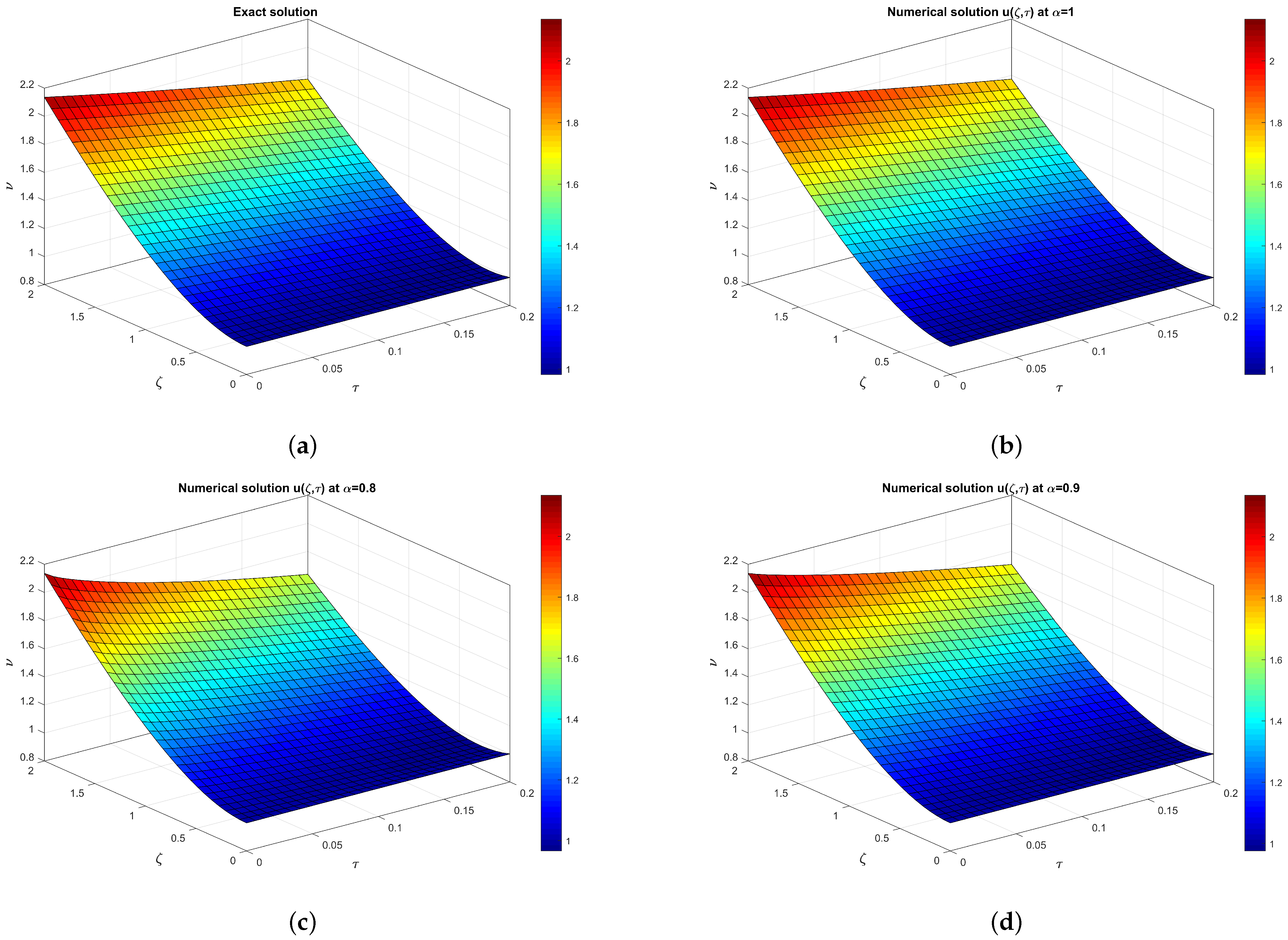
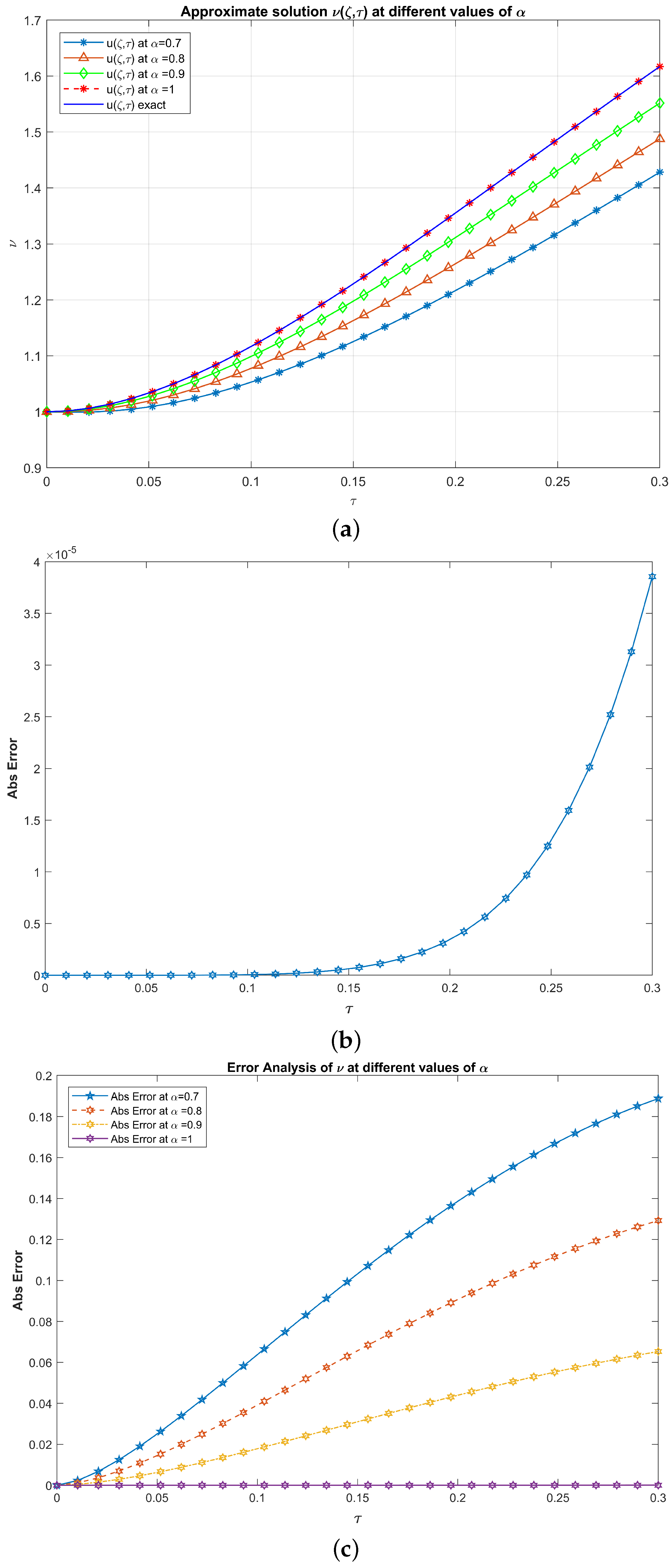
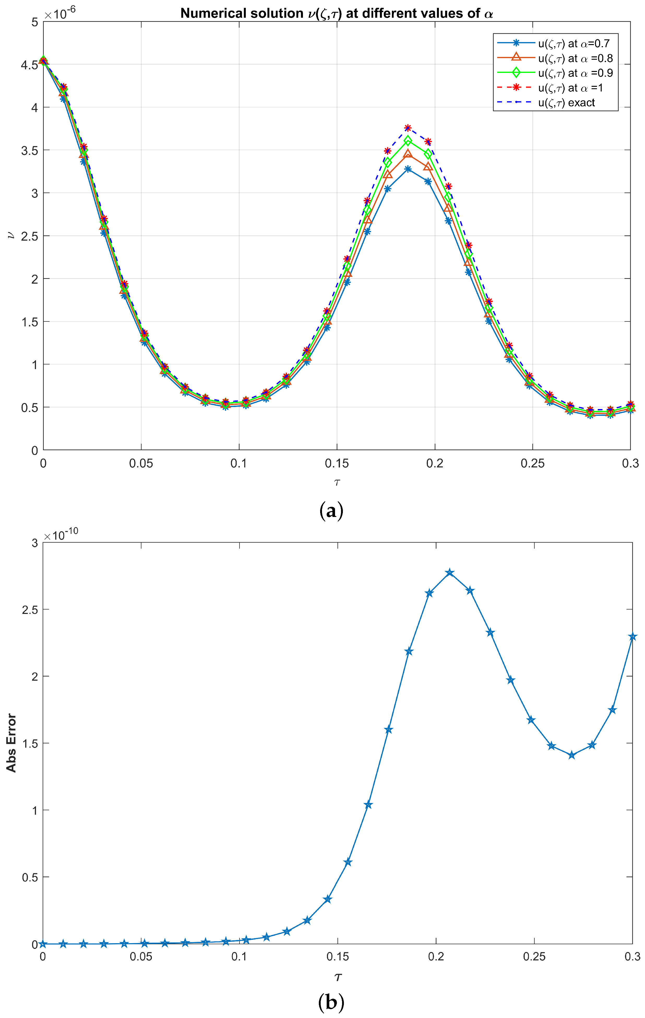
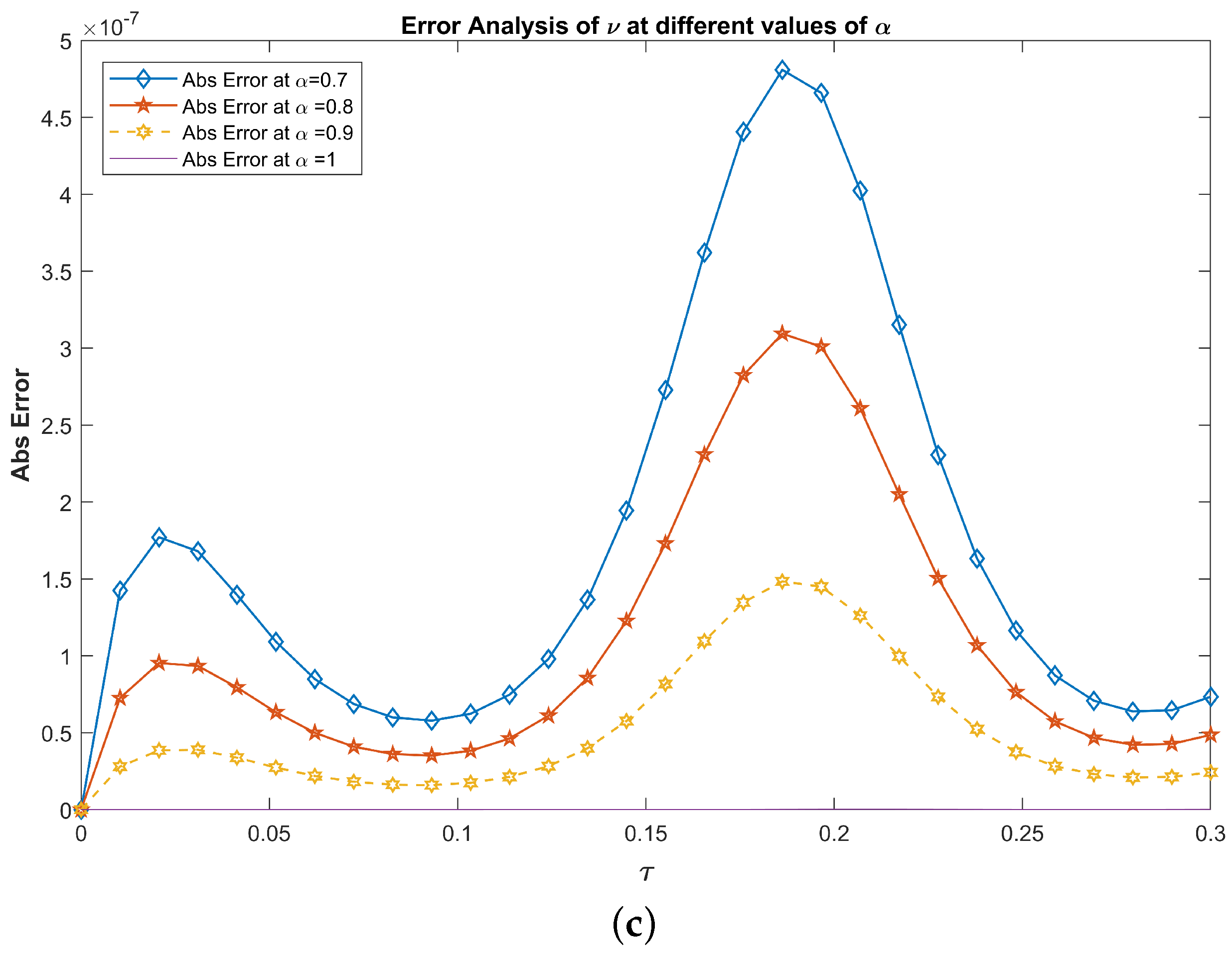
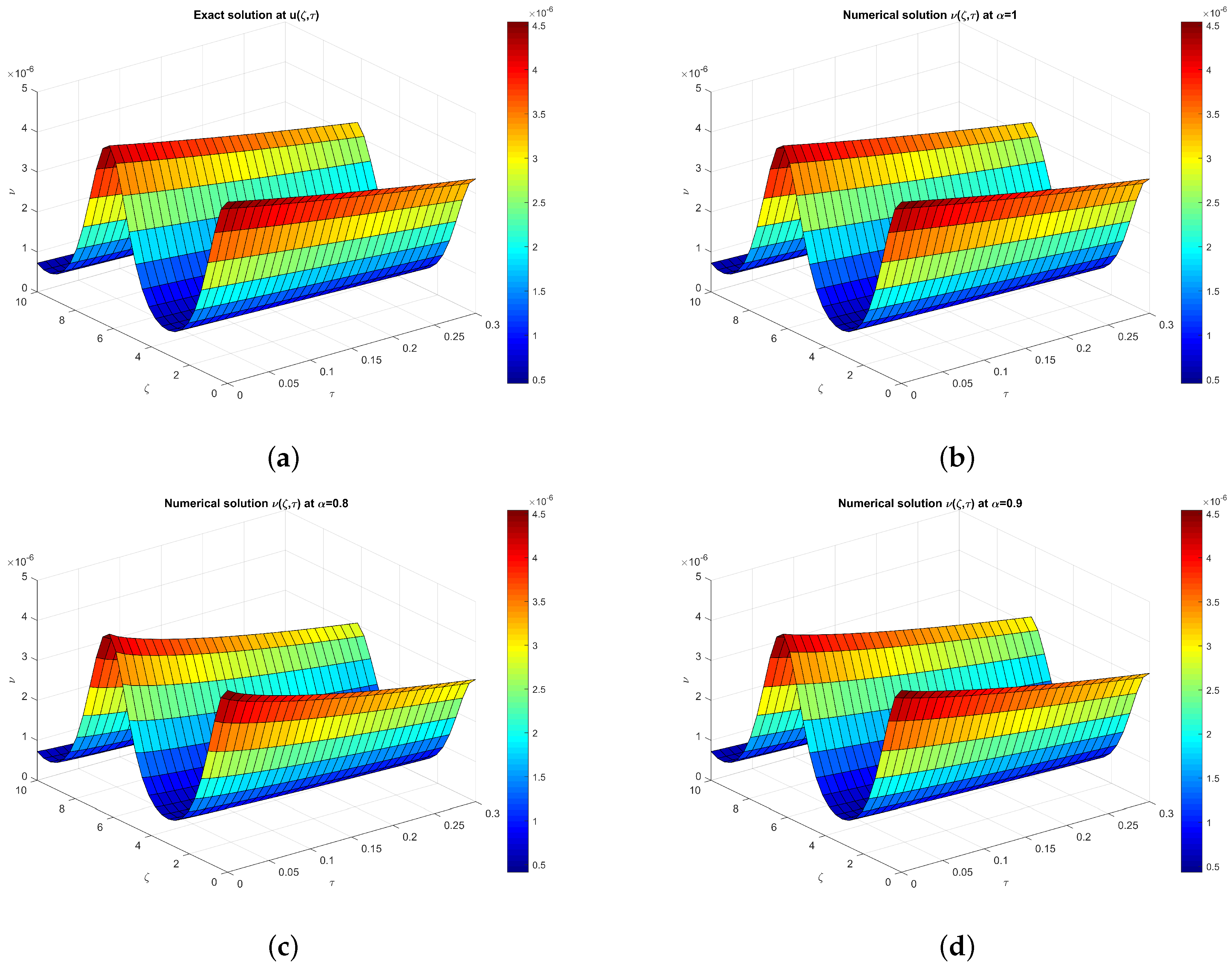
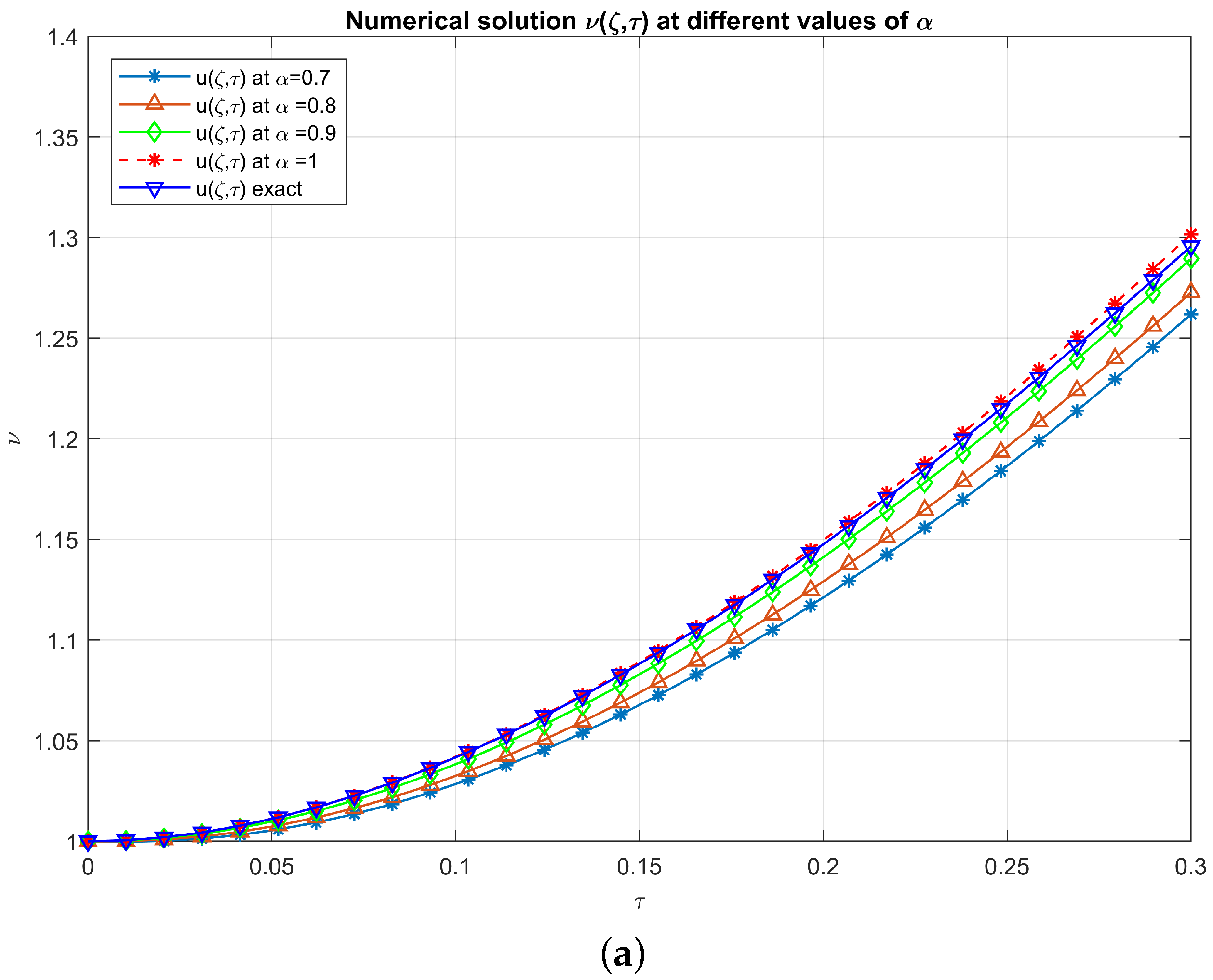
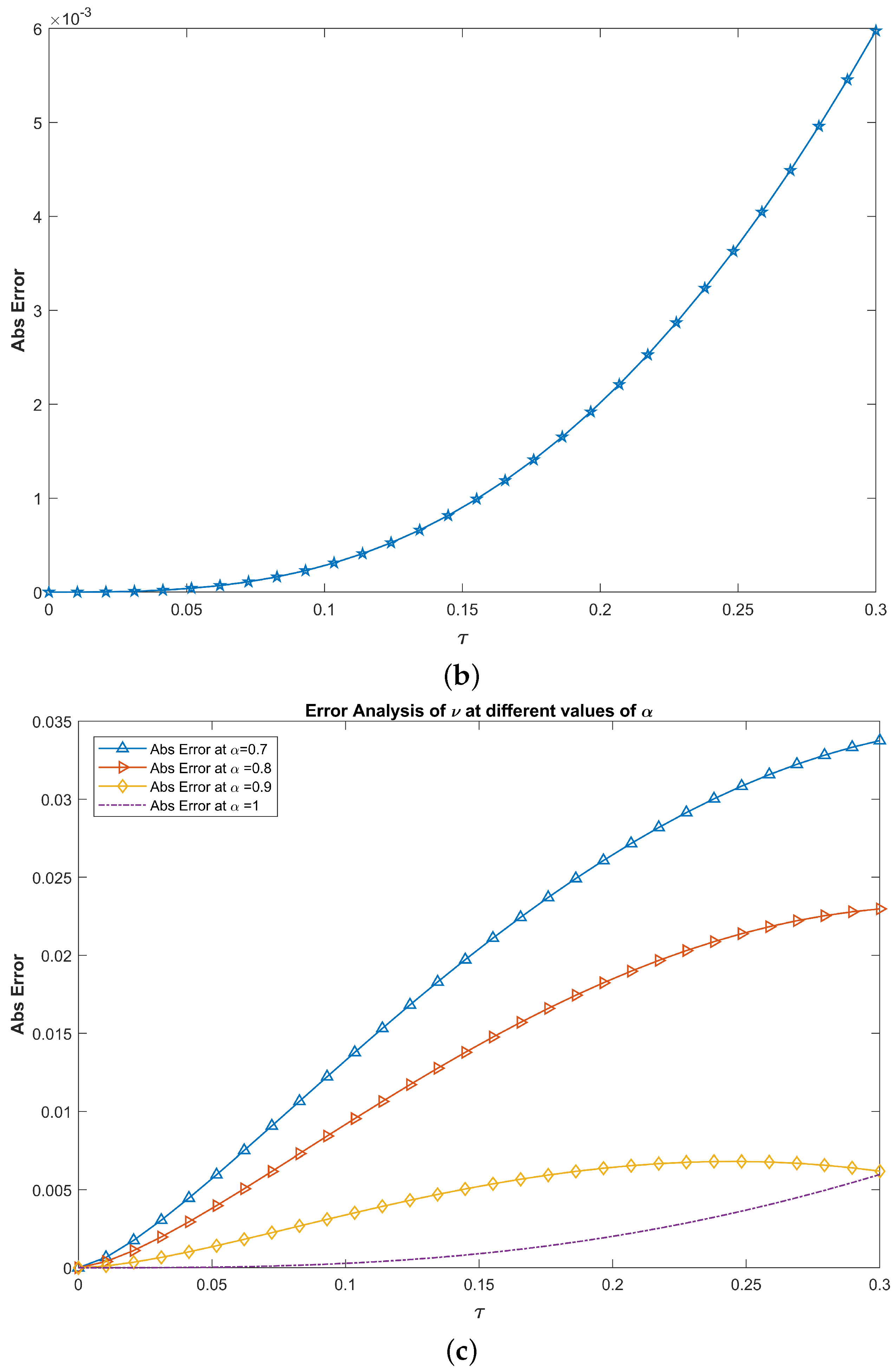
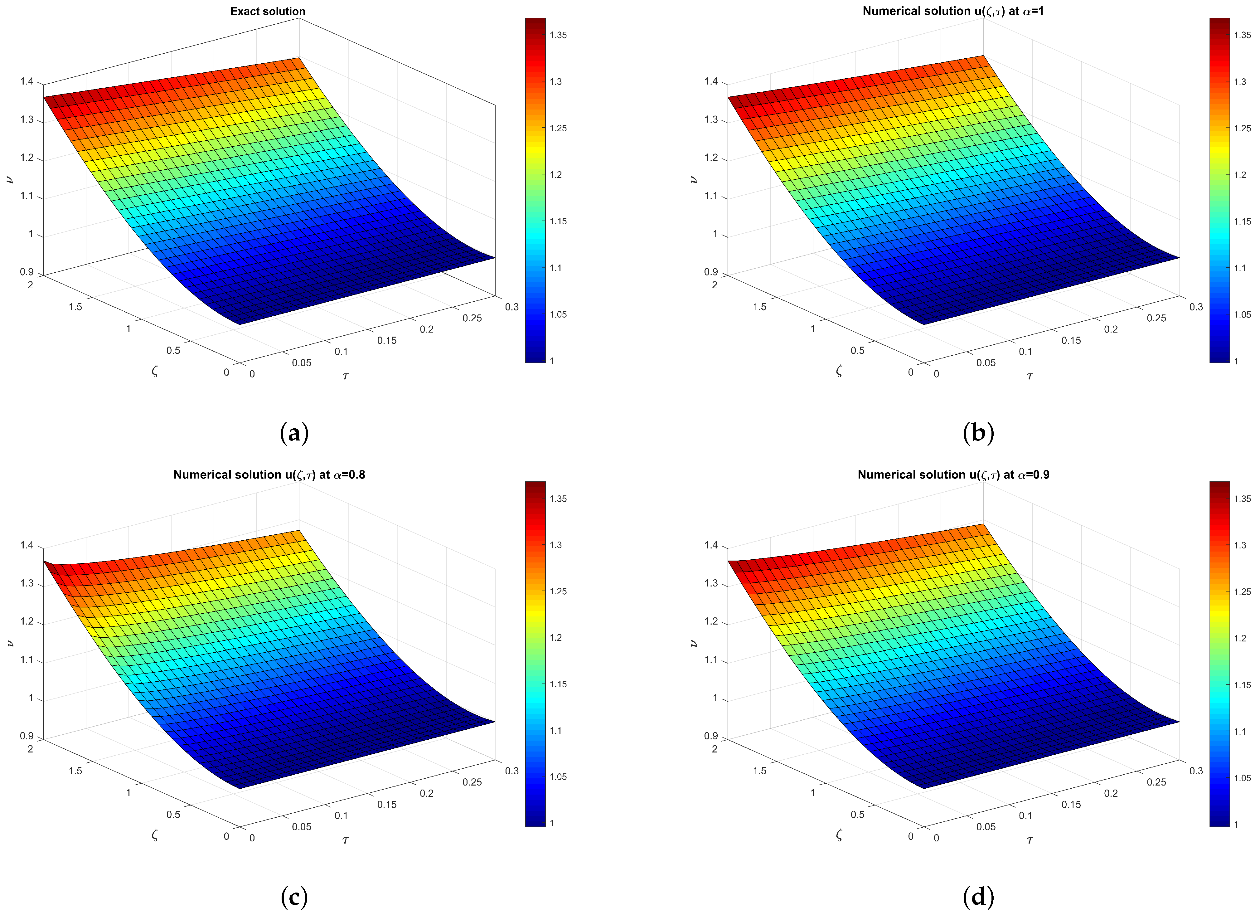
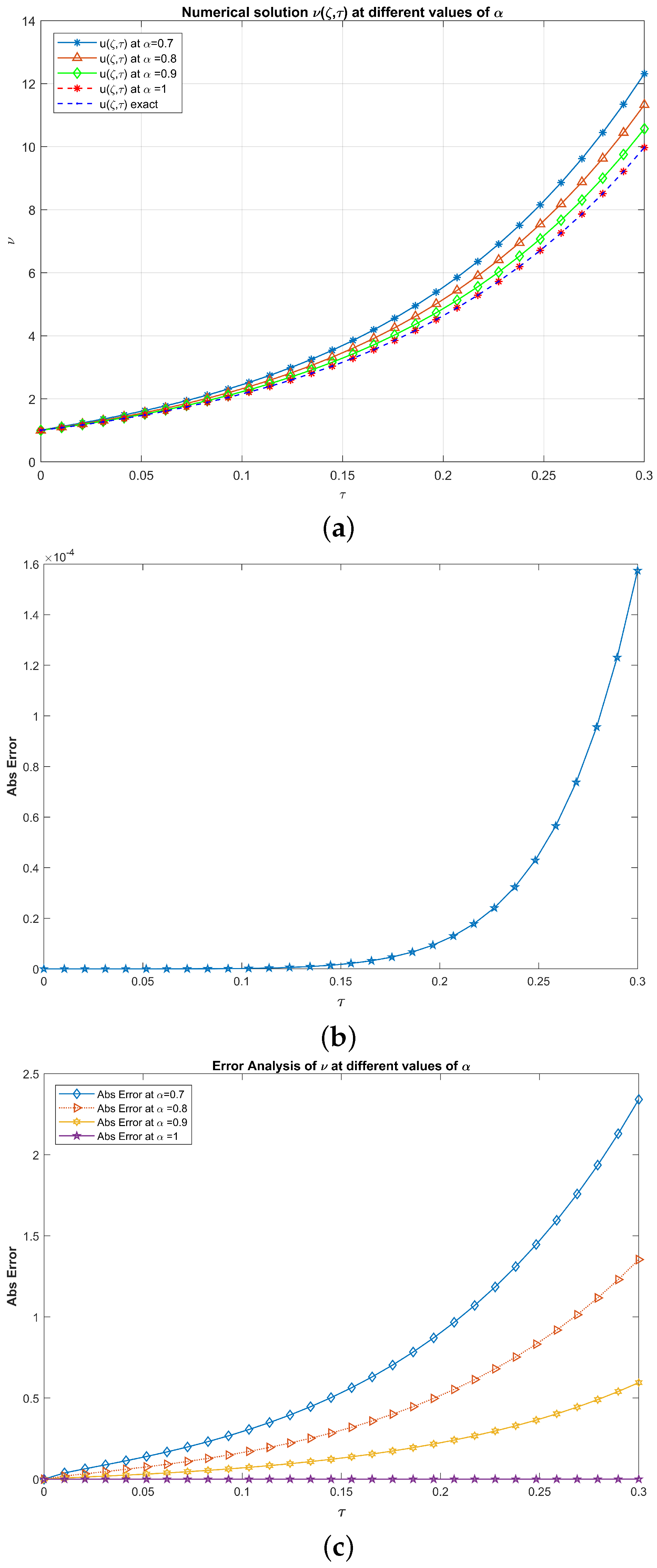
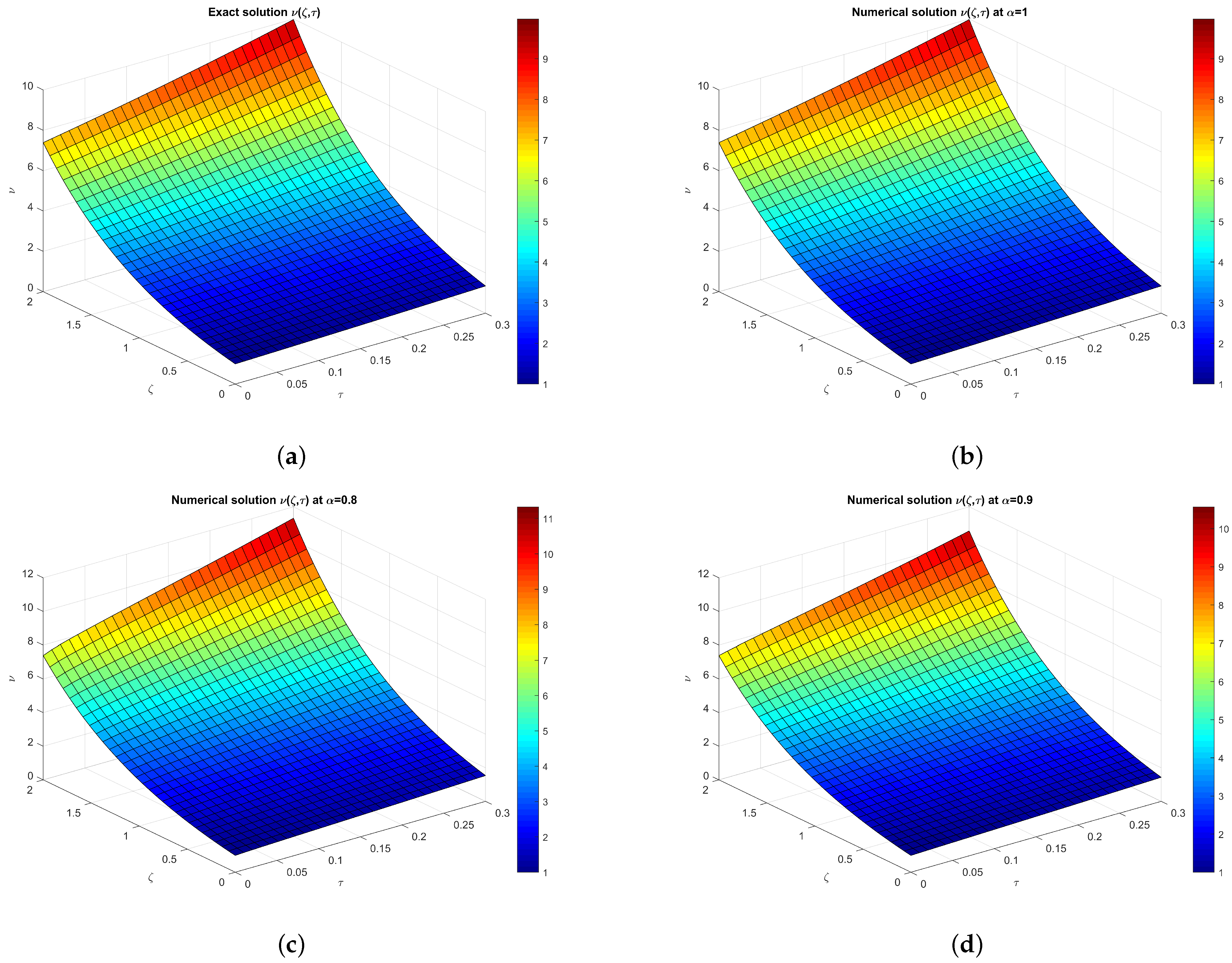
The numerical analysis involves the comparison of the approximate analytical solutions for various values of the fractional order (), where convergence to the exact solution is quick as the value of approaches 1. Moreover, the solutions are also presented in tabular form for a more detailed analysis.
The structure of the paper is as follows:
Section 2 will discuss the basic definitions and results used in the later discussion. In
Section 3, the methodology of the RPST method for solving TFC-DEqs will be discussed. Numerical examples verifying the proposed method are presented in
Section 4. Lastly,
Section 5 offers conclusive remarks emphasizing the efficacy of the method and presenting a convergence analysis, with
Section 6 summarizing the overall conclusions drawn from this study.
3. Residual Power Series Framework for Fractional Models
This section introduces a comprehensive methodology to solve TFC-DEqs. The problem we aim to solve is described in its general form by the following equations
with the initial condition (I.C.)
In this context,
is a function dependent on two variables, while
indicates the Caputo derivative of order
. Throughout this section, unless otherwise stated, we restrict the fractional parameter
to the interval
. Consequently, the integer-bound
m in Definition 2 is fixed at
.
The term
refers to a linear operator, and
denotes a non-linear operator. Additionally,
represents a non-homogeneous term. The RPST formulates the solution to Equation (
7) as a fractional power series expansion around the initial point at
:
In the above series expansion,
denotes the
th order coefficient function (or recursive component) of the solution, which depends exclusively on the spatial variable
. Since it is easier to deal with a finite series than an infinite series, the truncated series solution of Equation (
7) can be denoted
and expressed as
This can be written in an alternative way as
Here
=
is the initial approximate solution of
. The residual function associated with Equation (
7) is described as
Therefore, the
residual function can be stated as
To obtain the first approximation, take
in Equations (
11) and (
13) as
and by substituting Equation (
14) in Equation (
15), the residual function for the first approximation can be obtained as follows:
Finally by setting
allows us to get
In a similar way,
and so forth for
can be computed by implementing Equation (
11) in Equation (
13) and applying the following condition for
:
So, the general recurrence formula for computing the coefficients
is given as
Theorem 3 ([
32,
42])
. If the initial guess is contained inside the ball of the series solution , then the solution of (11) is convergent, whenever there exists an such that . Remark 1 ([
32,
42])
. The maximum truncation error of can be expressed as , where denotes the convergence ratio of the iterative series. Remark 2 (Intrinsic Handling of Non-linearities)
. A key operational advantage of the RPST is its capacity to by pass traditional linearization (e.g., Taylor series perturbation or Newton–Rapson iterations) and spatial discretization meshes. In classical methods, a nonlinear conective terms such as requires either a frozen coefficients approximation or discrete algebraic approximation over a grid.
In contrast, the RPST handles nonlinear terms directly through the systematic construction of the k-th order fractional residual function, . For a generalized nonlinear operator , the truncated expansionis substituted directly into the full nonlinear expression without modification. The core mechanism relies on evaluating the successive fractional derivatives of the residual exactly at the temporal origin () Because the evaluation is anchored at , all higher-order unknown expansion coefficients (for ) vanish identically due to the time dependency . Concurrently, the lower-order terms are already known from previous steps. Thus, when computing the k-th step, the nonlinear interaction resolves into a direct, linear algebraic combination of the known spatial derivatives from prior iterations. This enables the exact mapping of nonlinear cross-products into the next structural coefficient without requiring any simplifying assumptions, perturbation series, or artificial discretization parameters.