Sobolev-Type Neutral Stochastic Differential Equations with Hilfer Fractional Derivative and Finite Delay

Abstract

This study establishes the class of Sobolev-type neutral stochastic differential equations with Hilfer derivative and finite delay. Existence and uniqueness of the mild solution are then established in the mean-square sense via the Banach contraction principle, and a Faedo–Galerkin scheme is constructed whose approximate solutions are shown to converge, in mean square, to the unique mild solution. An application to a stochastically perturbed Sobolev-type filtering/diffusion model closes the paper.

1. Introduction

Fractional differential equations continue to attract sustained interest because the fractional derivative encodes memory and hereditary properties that ordinary derivatives cannot capture, with applications throughout fluid dynamics, viscoelasticity, population dynamics and signal processing. Fractional operators have also proved useful outside evolution equations themselves, for instance in approximation theory and special-function constructions [1,2]. The Caputo and Riemann–Liouville derivatives are the two most classical choices, but each imposes restrictions that are not always physically natural: the Caputo derivative requires the function itself (rather than a fractional integral of it) to be specified at the initial time, while the Riemann–Liouville derivative of a constant is generally non-zero and its associated initial-value problem is comparatively difficult to interpret physically. Hilfer [3] introduced a derivative ${}^{H}D_{0^{+}}^{\rho ,\sigma }$, depending on an order $\rho \in (0,1)$ and a type $\sigma \in [0,1]$, that interpolates continuously between the two classical derivatives and recovers each of them as a limiting case ($\sigma =0$ gives Riemann–Liouville, $\sigma =1$ gives Caputo). Existence theory for abstract evolution equations involving the Hilfer derivative was developed by Furati, Kassim and Tatar [4] and, in the setting of $C_0$-semigroups and mild solutions represented through generalized probability density (Mainardi–Wright) kernels, by Gu and Trujillo [5].

Independently, Sobolev-type equations in which a possibly non-invertible or unbounded operator $\mathcal{A}$ multiplies the highest order derivative, as in $\mathcal{A}{D}_{\vartheta }^{\rho }z=\mathcal{B}z+\cdots$ arise naturally in the control theory of dynamical systems, in flow through fissured rock, and in thermodynamics; see Debbouche and Nieto [6] for the Sobolev-type fractional nonlocal evolution equation and Kaliraj et al. [7,8] for the neutral, delayed and approximated Sobolev-type Caputo case that the present paper generalizes. Neutral equations, in which the derivative acts jointly on the state and on a functional g of the (possibly delayed) state, share properties with damped wave equations and are of independent interest.

At the same time, real systems are rarely free of random perturbation: model uncertainty, environmental noise and measurement error are naturally incorporated by driving the evolution equation with a Wiener process, leading to a stochastic evolution equation in a Hilbert space; the foundational theory is due to Da Prato and Zabczyk [9]. Stochastic fractional evolution equations combine memory effects with random perturbation and have been studied extensively for the Caputo derivative, but comparatively little is known in the Sobolev-type neutral case with a genuinely Hilfer derivative and finite delay.

On the nonlocal side, Byszewski [10] first showed that replacing the classical initial condition $z\left(0\right)=z_0$ by a nonlocal condition $z\left(0\right)+\phi \left(z\right)=z_0$ often gives a more realistic description of physical processes, for instance, when the initial state is measured indirectly or averaged over a time interval, and this observation has since been extended to essentially every class of fractional evolution equation, including the Sobolev-type Caputo neutral equation of [7] that we generalize here, and the abstract nonlocal Cauchy problem of Zhou and Jiao [11]. Existence results for fractional evolution equations are, almost without exception, proved via a fixed point technique (Banach, Krasnoselskii, Schauder, or Mönch), after the original evolution equation has first been rewritten, via a Laplace transform argument and a suitable probability density function, as an equivalent Volterra-type integral equation for the mild solution; this approach was pioneered for Caputo-type Sobolev equations by Debbouche and Nieto [6] and is precisely the approach we extend here to the Hilfer derivative and to the stochastic setting.

Stochastic fractional evolution equations have their own substantial literature. Mao’s monograph [12] remains the standard reference for finite-dimensional stochastic differential equations, while controllability and existence results for infinite-dimensional stochastic fractional evolution equations, typically with the Caputo derivative, have been obtained by Sakthivel, Ren and Mahmudov [13]. To the best of our knowledge, none of these papers treat the Hilfer derivative, the Sobolev-type operator pair $(\mathcal{A},\mathcal{B})$, the neutral structure (in which the fractional derivative acts on $\mathcal{A}z+g$ rather than on z alone), finite delay, and a genuinely infinite-dimensional Q-Wiener perturbation, all simultaneously; bringing these four features together is the contribution of the present manuscript. Beyond its own intrinsic interest, the Hilfer derivative is worth the additional generality because the type parameter $\sigma$ has a concrete interpretation: it interpolates the smoothing behavior of the associated resolvent family between the comparatively singular Riemann–Liouville extreme ($\sigma =0$, where $S_{\rho ,\sigma }\left(\vartheta \right)\sim {\vartheta }^{\rho -1}$ near $\vartheta =0$) and the bounded Caputo extreme ($\sigma =1$), so that $\sigma$ can be tuned, in applications such as viscoelastic or anomalous-diffusion models, to match the observed initial-time singularity of the data.

Very recently, and largely in parallel with the deterministic Sobolev-type programme of [7], a fast-growing body of work has begun to combine the Hilfer derivative with stochastic perturbations. Pradeesh and Vijayakumar [14] established existence and p-th moment asymptotic stability of mild solutions for Hilfer fractional neutral stochastic differential equations with infinite delay, and explicitly extended their system to the Sobolev type, which makes their paper the closest existing precedent to the present manuscript; unlike here, however, their delay is infinite (handled via a phase space) rather than finite, no Faedo–Galerkin approximation scheme is constructed, and the nonlocal condition is not treated. Related existence and controllability results for Hilfer (or $\psi$-Hilfer) fractional stochastic systems—with infinite delay and almost sectorial operators via the Mönch fixed point theorem [15], with impulses and nonlocal conditions via Krasnoselskii’s theorem [16], via measures of noncompactness [17], driven by a Rosenblatt rather than a Wiener process [18], via an averaging principle [19], and for stochastic differential inclusions [20]—have appeared very recently, but, like [14], none treats the finite delay, Sobolev-type, Faedo–Galerkin combination studied here. Gou [21] studied Sobolev-type Hilfer evolution equations with non-instantaneous impulses, and Gou and Li [22] obtained extremal mild solutions for Hilfer evolution equations with non-instantaneous impulses and nonlocal conditions using monotone iterative techniques; these two papers supply the non-stochastic, non-neutral counterpart of the operator-theoretic machinery (fractional powers of $\mathcal{E}$, generalized Mittag–Leffler resolvent families) that we adapt below to the neutral, delayed, stochastic setting. Relative to this literature, the present paper is, to our knowledge, the first to combine the Hilfer derivative, the Sobolev-type pair $(\mathcal{A},\mathcal{B})$, the neutral structure, finite delay, a nonlocal condition, and a genuine Q-Wiener perturbation simultaneously, together with a Faedo–Galerkin convergence theory and a new mean-square continuous-dependence result (Theorem 2).

Main contributions. In summary, this paper (i) formulates the Sobolev-type neutral stochastic differential equations (Equations (1)–(3)) with a genuinely Hilfer (rather than Caputo or Riemann–Liouville) fractional derivative, finite delay, and a nonlocal initial condition; (ii) derives the associated stochastic mild solution via a probability-density representation of the Hilfer resolvent families $S_{\rho ,\sigma }$, $T_{\rho }$ and proves its existence and uniqueness, in the mean-square sense, via the Banach contraction principle (Theorem 1); (iii) establishes mean-square continuous dependence of the mild solution on the nonlocal and delay data (Theorem 2), a result with no counterpart in the closest existing precedents; (iv) constructs a Faedo–Galerkin approximation scheme and proves its mean-square convergence to the mild solution (Theorems 4 and 5); and (v) verifies the full set of hypotheses on a concrete Sobolev-type stochastic heat/diffusion filtering model with an explicit admissible parameter choice (Section 5). Every one of the papers cited above is missing at least one of features (i)–(iv). The system (1)–(3) and the Hilfer derivative itself are formulated for the full range of type parameters $\sigma \in [0,1]$; as explained in Remark 5, the well-posedness and Faedo–Galerkin theory of Section 3 and Section 4 is developed for $\sigma =1$, where the resolvent bound of Lemma 1(i) is a genuine $\vartheta$-independent constant, and its extension to $\sigma <1$ via the standard weighted-space technique is left for future work.

The present manuscript closes this gap. We consider the neutral stochastic fractional differential equation (NSFDE) of Sobolev type

$$\begin{array}{cc}\hfill {}^{H}D_{0^{+}}^{\rho ,\sigma }\left[\mathcal{A}z\left(\vartheta \right)+g_0\left(\vartheta ,z\left(\vartheta \right),z\left(u_1\left(\vartheta \right)\right),\dots ,z\left(u_p\left(\vartheta \right)\right)\right)\right]& =\mathcal{B}z\left(\vartheta \right)+f_0\left(\vartheta ,z\left(\vartheta \right),z\left(u_1\left(\vartheta \right)\right),\dots ,z\left(u_p\left(\vartheta \right)\right)\right)\hfill \\ \hfill & +h_0\left(\vartheta ,z\left(\vartheta \right),z\left(u_1\left(\vartheta \right)\right),\dots ,z\left(u_p\left(\vartheta \right)\right)\right)\dot{W}\left(\vartheta \right),\vartheta \in (0,T],\hfill \end{array}$$

(1)

$$\begin{array}{cc}\hfill I_{0^{+}}^{(1-\rho )(1-\sigma )}\left[\mathcal{A}z+g_0(·,z(·),\dots ,z\left(u_p(·)\right))\right]\left(0^{+}\right)+{\phi }_0\left(z\right)& =\mathcal{A}\left[z_0+\mathsf{\Psi }\left(0\right)\right]+g_0\left(0,\mathsf{\Psi }\left(0\right),\dots ,\mathsf{\Psi }\left(u_p\left(0\right)\right)\right),\hfill \end{array}$$

(2)

$$\begin{array}{cc}\hfill z\left(\vartheta \right)& =z_0+\mathsf{\Psi }\left(\vartheta \right),\vartheta \in [-\eta ,0],\eta >0,\hfill \end{array}$$

(3)

where ${}^{H}D_{0^{+}}^{\rho ,\sigma }$ is the Hilfer fractional derivative of order $\rho \in (0,1)$ and type $\sigma \in [0,1]$, $\dot{W}$ denotes the formal white-noise derivative of a Q-Wiener process W on a Hilbert space K, ${\phi }_0$ is a nonlocal term generalizing the classical nonlocal condition, and $g_0,f_0,h_0$ are, respectively, the neutral, forcing, and diffusion maps of the problem (continuous, together with $u_i$). In (3), $\mathcal{A}:D\left(\mathcal{A}\right)\subset \mathrm{Y}\to \mathrm{Y}$ and $\mathcal{B}:D\left(\mathcal{B}\right)\subset \mathrm{Y}\to \mathrm{Y}$ are closed, positive, self-adjoint linear operators. The term $I_{0^{+}}^{(1-\rho )(1-\sigma )}$ denotes the Riemann–Liouville fractional integral of order $(1-\rho )(1-\sigma )$. As explained in Assumption 3 below, once the mild-solution Formula (8) is derived (Lemma 3), it is more convenient to work with the ${\mathcal{A}}^{-1}$-composed maps $g:={\mathcal{A}}^{-1}{g}_0,f:={\mathcal{A}}^{-1}{f}_0,h:={\mathcal{A}}^{-1}{h}_0,\phi :={\mathcal{A}}^{-1}{\phi }_0$, and from Section 2.4 onward (Assumptions 2–6 and everything thereafter) the unadorned symbols $g,f,h,\phi$ always refer to these composed maps, not to $g_0,f_0,h_0,{\phi }_0$ directly.

The rest of the paper is organized as follows. Section 2 will be utilized for the primary findings, including fractional calculus, fractional powers of the generator of an analytic compact semigroup, and the form of mild solutions of (3). Section 3 proves existence and uniqueness of the mild solution in the mean-square sense using the Banach fixed point theorem. Section 4 constructs the Faedo–Galerkin approximations and proves their mean-square convergence to the mild solution. Section 5 illustrates the abstract theory on a stochastically perturbed Sobolev-type filtering model, and Section 6 concludes.

2. Preliminaries

For quick reference, the “physical” neutral, forcing, diffusion, and nonlocal maps of the original problem (1) and (2) are always subscripted, $g_0,f_0,h_0,{\phi }_0$; the corresponding unsubscripted symbols $g:={\mathcal{A}}^{-1}{g}_0$, $f:={\mathcal{A}}^{-1}{f}_0$, $h:={\mathcal{A}}^{-1}{h}_0$, $\phi :={\mathcal{A}}^{-1}{\phi }_0$ denote the same maps composed with the bounded operator ${\mathcal{A}}^{-1}$ of (C3), and it is exclusively the unsubscripted, composed maps that appear in the mild-solution Formula (8), in Assumptions 2–6, and in every result from Section 3 onward. Assumption 3 below records the precise (routine) relationship between the two sets of constants; the reader who is only interested in Section 3, Section 4 and Section 5 may simply read $g,f,h,\phi$ throughout as “the (already composed) maps subject to Assumptions 2–6” without needing to track ${\mathcal{A}}^{-1}$ explicitly.

2.1. Function Spaces and the Operators $\mathcal{A},\mathcal{B}$

Let $(\mathrm{Y},∥·∥)$ be a Hilbert space and let $\mathcal{A}:D\left(\mathcal{A}\right)\subset \mathrm{Y}\to \mathrm{Y}$, $\mathcal{B}:D\left(\mathcal{B}\right)\subset \mathrm{Y}\to \mathrm{Y}$ be closed, positive, self-adjoint linear operators satisfying the following:

(C1)

$\mathcal{A},\mathcal{B}$ are linear and closed.

(C2)

$D\left(\mathcal{A}\right)\subset D\left(\mathcal{B}\right)$ and $\mathcal{A}$ is bijective.

(C3)

${\mathcal{A}}^{-1}:\mathrm{Y}\to D\left(\mathcal{A}\right)\subset \mathrm{Y}$ is linear and continuous, $Im\left({\mathcal{A}}^{-1}\right)\subset D\left(\mathcal{B}\right)$, $Im\left(\mathcal{B}\right)\subset D\left({\mathcal{A}}^{-1}\right)$, and $\mathcal{B}{\mathcal{A}}^{-1}={\mathcal{A}}^{-1}\mathcal{B}$.

By the closed graph theorem, $\mathcal{E}:=\mathcal{B}{\mathcal{A}}^{-1}$, with domain $D\left(\mathcal{E}\right)\subset \mathrm{Y}\to \mathrm{Y}$, is a bounded linear operator on $\mathrm{Y}$: ${\mathcal{A}}^{-1}$ is bounded and everywhere defined by (C3), and $\mathcal{E}$ is closed (if $x_n\to x$ and $\mathcal{E}{x}_n\to y$ then ${\mathcal{A}}^{-1}{x}_n\to {\mathcal{A}}^{-1}x$ by boundedness, so $\mathcal{B}{\mathcal{A}}^{-1}{x}_n\to y$ with $\mathcal{B}$ closed forces ${\mathcal{A}}^{-1}x\in D\left(\mathcal{B}\right)$ and $\mathcal{E}x=y$); a closed operator defined on all of $\mathrm{Y}$ is bounded by the closed graph theorem. Being bounded, $\mathcal{E}$ generates a uniformly continuous (in particular $C_0$) semigroup ${\left\{S\left(\vartheta \right)\right\}}_{\vartheta \ge 0}$, $S\left(\vartheta \right):=e^{\mathcal{E}\vartheta }$, via the exponential series—this much, and only this much, follows from the closed graph theorem. It does not give a uniform-in-$\vartheta$ bound on $∥S\left(\vartheta \right)∥$: since $\mathcal{E}$ is positive self-adjoint by Assumption 1, in fact $∥S\left(\vartheta \right)∥={sup}_i{e}^{{\alpha }_i\vartheta }\to \infty$ as $\vartheta \to \infty$ for $S\left(\vartheta \right)=e^{\mathcal{E}\vartheta }$ taken literally. Since only the finite horizon $\vartheta \in [0,T]$ is ever used below, this is not a genuine obstruction: $\vartheta \mapsto S\left(\vartheta \right)$ is continuous on the compact interval $[0,T]$, so

$$N_0:=\underset{\vartheta \in [0,T]}{sup}∥S\left(\vartheta \right)∥<\infty$$

(4)

holds automatically, with no further hypothesis, and this is the only bound on S used anywhere in Section 2, Section 3 and Section 4 below (in particular in Lemma 1(i)). We record it as $N_0$; this is a finite-T bound, not the stronger $\vartheta \to \infty$ statement that a literal reading of “closed graph theorem ⇒ uniformly bounded semigroup” would suggest; the latter would additionally require $\Re (spec(\mathcal{E}\left)\right)\le 0$ (Hille–Yosida), which fails here since $\mathcal{E}>0$, and is not needed for any result in this paper. $W_1:=∥{\mathcal{A}}^{-1}∥$. We assume:

Assumption 1. 

$\mathcal{E}$ has a pure point spectrum $0<{\alpha }_0\le {\alpha }_1\le \cdots \le {\alpha }_m\le \cdots$ with a complete orthonormal system of eigenfunctions ${\left\{{\chi }_i\right\}}_{i\ge 0}$, $\mathcal{E}{\chi }_i={\alpha }_i{\chi }_i$, and ${\chi }_i$ is also an eigenfunction of $\mathcal{A}$ and of $\mathcal{B}$ for every i (equivalently, $\mathcal{A},\mathcal{B},\mathcal{E}$ are simultaneously diagonalized by $\left\{{\chi }_i\right\}$; this holds automatically whenever $\mathcal{A},\mathcal{B}$ are both functions of a single underlying self-adjoint operator with compact resolvent, as in the concrete example of Section The Faedo–Galerkin Scheme, and is needed below so that the finite-dimensional projections $P^n$ built from $\left\{{\chi }_i\right\}$ commute with $\mathcal{A},\mathcal{B},\mathcal{E}$ and with the fractional power ${\mathcal{E}}^{\beta }$ of Assumption 2). We do not assume ${\alpha }_i\to \infty$: the sequence $\left\{{\alpha }_i\right\}$ may converge to a finite limit, as it does in the concrete Sobolev-type example of Section The Faedo–Galerkin Scheme, where $\mathcal{E}$ is a bounded operator; the Faedo–Galerkin convergence theory of Section 4 is stated so as to remain valid in that case (Remark 8 below).

For $0\le \mu <1$, the fractional power ${\mathcal{E}}^{\mu }$ is well defined on $D\left({\mathcal{E}}^{\mu }\right)$, which is a Banach space (in fact, a Hilbert space) under ${∥z∥}_{\mu }=∥{\mathcal{E}}^{\mu }z∥$; we write ${\mathrm{Y}}_{\mu }:=D\left({\mathcal{E}}^{\mu }\right)$.

2.2. Stochastic Framework

Let $(\mathsf{\Omega },\mathcal{F},{\left\{{\mathcal{F}}_{\vartheta }\right\}}_{\vartheta \ge 0},\mathbb{P})$ be a complete filtered probability space and let $W={\left\{W\left(\vartheta \right)\right\}}_{\vartheta \ge 0}$ be a Q-Wiener process on a separable Hilbert space K, with Q a non-negative, self-adjoint, finite-trace operator on K, adapted to $\left\{{\mathcal{F}}_{\vartheta }\right\}$. Let $L_2^0:=L_2(Q^{1/2}K,\mathrm{Y})$ denote the space of Hilbert–Schmidt operators from $Q^{1/2}K$ into $\mathrm{Y}$, equipped with ${∥\mathsf{\Phi }∥}_{L_2^0}^2=tr\left(\mathsf{\Phi }Q{\mathsf{\Phi }}^{*}\right)$; stochastic integrals ${\int }_0^{\vartheta }\mathsf{\Phi }\left(s\right)dW\left(s\right)$ for $L_2^0$-valued, predictable, square-integrable $\mathsf{\Phi }$ satisfy the Itô isometry

$$\mathbb{E}\parallel {\int }_0^{\vartheta }\mathsf{\Phi }\left(s\right)dW\left(s\right){\parallel }^2={\int }_0^{\vartheta }\mathbb{E}{∥\mathsf{\Phi }\left(s\right)∥}_{L_2^0}^{2}ds.$$

(5)

For $0\le \mu \le 1$, define the weighted, mean-square Banach space of ${\mathcal{F}}_{\vartheta }$-adapted continuous processes

$$D_T^{\mu }=\left\{z:[-\eta ,T]\to {\mathrm{Y}}_{\mu },z\mathrm{is}\left\{{\mathcal{F}}_{\vartheta }\right\}-\mathrm{adapted},\mathrm{continuous}\mathrm{on}[-\eta ,T],\underset{s\in [-\eta ,T]}{sup}\mathbb{E}{∥z\left(s\right)∥}_{\mu }^2<\infty \right\},$$

normed by ${∥z∥}_{T,\mu }^2={sup}_{s\in [-\eta ,T]}\mathbb{E}{∥z\left(s\right)∥}_{\mu }^2$; $D_T^{\mu }$ is a complete metric space under this norm (the paths are continuous, not merely càdlàg, since the system (1)–(3) has no impulsive/jump component).

Set

$$\tilde{\mathsf{\Psi }}\left(\vartheta \right)=\left\{\begin{array}{cc}{z}_0+\mathsf{\Psi }\left(\vartheta \right),\hfill & \vartheta \in [-\eta ,0],\hfill \\ z_0+\mathsf{\Psi }\left(0\right),\hfill & \vartheta \in [0,T],\hfill \end{array}\right.B_R(D_T^{\mu },\tilde{\mathsf{\Psi }})=\{z\in D_T^{\mu }:{∥z-\tilde{\mathsf{\Psi }}∥}_{T,\mu }\le R\},R>0.$$

2.3. The Hilfer Fractional Derivative

Definition 1 

([3]). Let $\rho \in (0,1)$, $\sigma \in [0,1]$ and $\gamma =\rho +\sigma -\rho \sigma$. The Hilfer fractional derivative of order ρ and type σ of a function z is

$${}^{H}D_{0^{+}}^{\rho ,\sigma }z\left(\vartheta \right)=I_{0^{+}}^{\sigma (1-\rho )}{\displaystyle \frac{d}{d\vartheta }}{I}_{0^{+}}^{(1-\sigma )(1-\rho )}z\left(\vartheta \right),$$

where $I_{0^{+}}^{\nu }z\left(\vartheta \right)={\displaystyle \frac{1}{\mathsf{\Gamma }\left(\nu \right)}}{\int }_0^{\vartheta }{(\vartheta -s)}^{\nu -1}z\left(s\right)ds$ is the Riemann–Liouville fractional integral of order $\nu >0$. When $\sigma =1$, ${}^{H}D_{0^{+}}^{\rho ,\sigma }$ coincides with the Caputo derivative ^c$D_{\vartheta }^{\rho }$; when $\sigma =0$ it coincides with the Riemann–Liouville derivative.

2.4. Standing Hypotheses

Throughout the paper we fix parameters $0<\beta <\mu <1$ and $\rho \in (0,1)$ subject to the single admissibility constraint

$$\rho (1-\mu )>\frac{1}{2},$$

(6)

which is needed for the near-diagonal integrability of the squared kernel appearing in the Itô-isometry estimates of Assumption 5 below (see Remark 4 after Lemma 1); this is a genuine restriction on the pair $(\rho ,\mu )$, not an automatic consequence of $\rho ,\mu \in (0,1)$ (it fails, e.g., for $\rho$ close to 0, whatever $\mu$ is, or for $\mu$ close to 1 with $\rho <1$), and must be checked in any application.

In addition, and only from this point on—the general Hilfer derivative ${}^{H}D_{0^{+}}^{\rho ,\sigma }$ with $\sigma \in [0,1]$ is defined, and Lemma 1(i) below is stated, for arbitrary $\sigma \in [0,1]$—we fix the type parameter at $\sigma =1$ for the well-posedness and approximation theory of Section 3 and Section 4 (Theorems 1, 2, 4 and 5) and for the worked example of Section 5. The reason is made precise in Remark 5 after Lemma 1: the bound of Lemma 1(i) is genuinely $\vartheta$-independent only when $\sigma =1$, and it is exactly this $\vartheta$-independent constant K that is used as a uniform bound in (20) and (21) and throughout the proofs of Section 3 and Section 4. Definitions and statements that do not rely on this uniform bound (the Hilfer derivative itself, and Lemma 1(i) as a pointwise estimate) are kept in their natural generality, $\sigma \in [0,1]$.

Remark 1 

(Practical range of $(\rho ,\mu )$). Condition (6) restricts the pair $(\rho ,\mu )$ to the region $\{(\rho ,\mu )\in {(0,1)}^2:\mu <1-\frac{1}{2\rho }\}$, which is non-empty exactly for $\rho >1/2$ and shrinks as $\rho \downarrow 1/2$; for $\rho \le 1/2$ no admissible $\mu \in (0,1)$ exists at all, since then $\rho (1-\mu )<\rho \le 1/2$ for every $\mu >0$. Concretely, for $\rho =0.9$, any $\mu \in (0,1-\frac{1}{1.8})=(0,0.444)$ is admissible (e.g., $\mu =0.3$, and then any $\beta \in (0,\mu )$, e.g., $\beta =0.1$); for $\rho =0.6$, only $\mu \in (0,0.167)$ is admissible; and $\rho =0.5$ admits no $\mu >0$ at all. In practice, since ρ close to 1 makes the Hilfer derivative closest to a classical (integer-order) derivative while μ close to 0 corresponds to the mildest fractional-power regularity requirement on $g,f,h$, condition (6) is easiest to satisfy, and hence least restrictive on the class of nonlinearities covered, when ρ is taken close to 1; it becomes progressively more restrictive as $\rho \downarrow 1/2$ and is simply infeasible for $\rho \le 1/2$, for any type $\sigma \in [0,1]$ (the constraint does not involve σ at all, cf. Remark 4). The explicit choice used in the worked example of Section A Concrete Sobolev-Type Stochastic Heat/Diffusion Example below is $\rho =0.9$, $\mu =0.3$, $\beta =0.1$, $\sigma =1$.

Assumption 2. 

There is a continuous map ${\mathcal{E}}^{\beta }g:[0,T]\times {\mathrm{Y}}_{\mu }^{p+1}\to \mathrm{Y}$ and, for each $r>0$, a constant $L_g\left(r\right)>0$ such that

$$\mathbb{E}{∥{\mathcal{E}}^{\beta }g({\vartheta }_1,z_1,\dots ,z_{p+1})-{\mathcal{E}}^{\beta }g({\vartheta }_2,w_1,\dots ,w_{p+1})∥}^2\le L_g\left(r\right)\left[|{\vartheta }_1-{\vartheta }_2{|}^2+{\displaystyle \sum _{i=1}^{p+1}}\mathbb{E}{∥z_i-w_i∥}_{\mu }^2\right]$$

for all $(z_1,\dots ,z_{p+1}),(w_1,\dots ,w_{p+1})\in B_R{(D_T^{\mu },\tilde{\mathsf{\Psi }})}^{p+1}$, ${\vartheta }_1,{\vartheta }_2\in [0,T]$.

Assumption 3. 

Throughout the paper, the symbols $g,f,h,\phi$ appearing in (1), (2), (8) and in Assumptions 2–6 denote the maps ${\mathcal{A}}^{-1}{g}_0,{\mathcal{A}}^{-1}{f}_0,{\mathcal{A}}^{-1}{h}_0,{\mathcal{A}}^{-1}{\phi }_0$, where $g_0,f_0,h_0,{\phi }_0$ are the (possibly distinct) neutral, forcing, diffusion, and nonlocal maps as they appear literally in the underlying physical problem, and ${\mathcal{A}}^{-1}$ is the bounded operator of (C3). This is a matter of notation, not an approximation: ${\mathcal{A}}^{-1}$ is not the identity in general (if $\mathcal{A}{\chi }_i=a_i{\chi }_i$ then ${\mathcal{A}}^{-1}{\chi }_i=a_i^{-1}{\chi }_i\ne {\chi }_i$, e.g., $a_i=1+i^2$ in the concrete example of Section The Faedo–Galerkin Scheme), but it is a bounded linear operator ($∥{\mathcal{A}}^{-1}∥=W_1<\infty$ by (C3)), and boundedness alone is enough for our purposes: if $g_0$ satisfies the Lipschitz/growth bound of Assumption 2 with constant $L_{g_0}\left(r\right)$, then $g={\mathcal{A}}^{-1}{g}_0$ satisfies the same type of bound, with constant $L_g\left(r\right)\le W_1^2{L}_{g_0}\left(r\right)$ (since $\mathbb{E}{∥{\mathcal{A}}^{-1}(g_0(z_1,\dots )-g_0(w_1,\dots ))∥}^2\le W_1^2\mathbb{E}{∥g_0(z_1,\dots )-g_0(w_1,\dots )∥}^2$), and likewise for $f,h,\phi$. We therefore state Assumptions 2–6 directly in terms of the (already ${\mathcal{A}}^{-1}$-composed) maps $g,f,h,\phi$, with constants $L_g,L_f,L_h,C_{\phi }$ understood to be $\le W_1^2$ times the corresponding constants for $g_0,f_0,h_0,{\phi }_0$. No further hypothesis is needed: ${\mathcal{A}}^{-1}$ appears nowhere else in the mild-solution Formula (8) or in Section 3, Section 4 and Section 5 below, since it has already been absorbed into the definition of $g,f,h,\phi$ used throughout.

Assumption 4. 

$f:[0,T]\times {\mathrm{Y}}_{\mu }^{p+1}\to \mathrm{Y}$ is continuous and there is a non-decreasing $L_f:{\mathbb{R}}^{+}\to {\mathbb{R}}^{+}$ with

$$\begin{array}{cc}\hfill \mathbb{E}{∥f({\vartheta }_1,z_1,\dots ,z_{p+1})-f({\vartheta }_2,w_1,\dots ,w_{p+1})∥}^2& \le L_f\left(r\right)\left[|{\vartheta }_1-{\vartheta }_2{|}^2+{\displaystyle \sum _{i=1}^{p+1}}\mathbb{E}{∥z_i-w_i∥}_{\mu }^2\right],\hfill \\ \hfill \mathbb{E}{∥f(\vartheta ,z_1,\dots ,z_{p+1})∥}^2& \le L_f\left(\vartheta \right),\hfill \end{array}$$

for all $(z_1,\dots ,z_{p+1}),(w_1,\dots ,w_{p+1})\in B_R{(D_T^{\mu },\tilde{\mathsf{\Psi }})}^{p+1}$, ${\vartheta }_1,{\vartheta }_2\in [0,T]$.

Assumption 5. 

$h:[0,T]\times {\mathrm{Y}}_{\mu }^{p+1}\to L_2^0$ is continuous and there is a non-decreasing $L_h:{\mathbb{R}}^{+}\to {\mathbb{R}}^{+}$ with

$$\begin{array}{cc}\hfill \mathbb{E}{∥h({\vartheta }_1,z_1,\dots ,z_{p+1})-h({\vartheta }_2,w_1,\dots ,w_{p+1})∥}_{L_2^0}^2& \le L_h\left(r\right)\left[|{\vartheta }_1-{\vartheta }_2{|}^2+{\displaystyle \sum _{i=1}^{p+1}}\mathbb{E}{∥z_i-w_i∥}_{\mu }^2\right],\hfill \\ \hfill \mathbb{E}{∥h(\vartheta ,z_1,\dots ,z_{p+1})∥}_{L_2^0}^2& \le L_h\left(\vartheta \right),\hfill \end{array}$$

for all $(z_1,\dots ,z_{p+1}),(w_1,\dots ,w_{p+1})\in B_R{(D_T^{\mu },\tilde{\mathsf{\Psi }})}^{p+1}$, ${\vartheta }_1,{\vartheta }_2\in [0,T]$. The near-diagonal integrability condition (6), $\rho (1-\mu )>1/2$, fixed above, is what makes the squared kernel ${(\vartheta -s)}^{2(\rho -1)}{∥{\mathcal{E}}^{\mu }{T}_{\rho }(\vartheta -s)∥}^2$ appearing in the Itô-isometry estimates below integrable near $s=\vartheta$, which is required throughout Section 3 and Section 4 (see Remark 4).

Assumption 6. 

The nonlocal map $\phi \in C(D_T^{\mu },{\mathrm{Y}}_{\mu })$ is defined on the trajectory space $D_T^{\mu }$—consistently with its use in (2) and (8), where $\phi \left(z\right)$ depends on the entire path $z:[-\eta ,T]\to {\mathrm{Y}}_{\mu }$ (e.g., through finitely many point-evaluations $z\left({\vartheta }_j\right)$, as in the multiple-point nonlocal condition of Section A Concrete Sobolev-Type Stochastic Heat/Diffusion Example rather than on a single value $z\left(\vartheta \right)\in {\mathrm{Y}}_{\mu }$—and satisfies, for a constant $C_{\phi }>0$,

$$\mathbb{E}{∥\phi \left(z_1\right)-\phi \left(z_2\right)∥}_{\mu }^2\le C_{\phi }{∥z_1-z_2∥}_{T,\mu }^2:=C_{\phi }\underset{\vartheta \in [-\eta ,T]}{sup}\mathbb{E}{∥z_1\left(\vartheta \right)-z_2\left(\vartheta \right)∥}_{\mu }^2,z_1,z_2\in D_T^{\mu }.$$

This is the same trajectory-space Lipschitz norm ${∥·∥}_{T,\mu }$ already used throughout Section 3 and Section 4 (see, e.g., (20) via $I_1$, and Theorem 2), so no new space is introduced; only the domain on which φ is declared to act has been made explicit and consistent with the rest of the paper.

Assumption 7. 

$u_i:[0,T]\to [0,T]$ are continuous with $0\le u_i\left(\vartheta \right)\le \vartheta$, $\vartheta \in [0,T]$, $i=1,\dots ,p$; $\mathsf{\Psi }\in D\left(\mathcal{E}\right)$ is ${\mathcal{F}}_0$-measurable with $\mathbb{E}{∥\mathsf{\Psi }∥}_{0,\mu }^2<\infty$.

Remark 2 

(Which assumption is used where). 

Table 1. Hypotheses used in each main result.

Result	Hypotheses Used
Lemma 3 (mild-solution formula)	Assumption 1
Theorem 1 (existence/uniqueness)	Assumptions 1–7, (6), (20) and (21)
Theorem 2 (continuous dependence)	Assumptions 1–7, (20) and (21)
Theorem 3 ($F_n$ has a fixed point $z_n$)	Assumptions 1–7, (20) and (21)
Lemma 4 (n-uniform bound on $z_n$)	hypotheses of Theorem 3, plus $\mathsf{\Psi }\left(\vartheta \right)\in D\left(\mathcal{E}\right)$
Theorem 4 ($z_n\to z$)	hypotheses of Lemma 4
Theorem 5 (${\overline{z}}_n\to z$)	Assumptions 1–7, (20) and (21), $\mathsf{\Psi }\left(\vartheta \right)\in D\left(\mathcal{E}\right)$

summarizes which of Assumptions 1–7 and which of conditions (6), (20) and (21) are invoked in each of the main theorems, to help the reader track the logical dependencies without re-reading every proof in full.

In particular, the admissibility restriction (6) enters only through the Itô-isometry integrability of Assumption 5 (Remark 4); every other hypothesis in the table is independent of the specific pair $(\rho ,\mu )$ chosen, subject to (6) itself.

2.5. The Stochastic Mild Solution

Following the Hilfer semigroup approach of Gu and Trujillo [5] together with the probability-density technique used for the Caputo case in ([7], Lemma 2.2), define the one-sided stable density

$$P_{\rho }\left(\theta \right)={\displaystyle \frac{1}{\pi }}{\displaystyle \sum _{n=1}^{\infty }}{(-1)}^{n-1}{\theta }^{-n\rho -1}{\displaystyle \frac{\mathsf{\Gamma }(n\rho +1)}{n!}}sin\left(n\pi \rho \right),\theta \in (0,\infty ),$$

and the associated probability density function ${\chi }_{\rho }\left(\theta \right)=\rho {\theta }^{-1-1/\rho }{P}_{\rho }\left({\theta }^{-1/\rho }\right)$, so that ${\int }_0^{\infty }{\chi }_{\rho }\left(\theta \right)d\theta =1$. Define the operator families

$$K_{\rho }\left(\vartheta \right)={\vartheta }^{\rho -1}{T}_{\rho }\left(\vartheta \right),T_{\rho }\left(\vartheta \right)={\int }_0^{\infty }\rho \theta {\chi }_{\rho }\left(\theta \right)S\left({\vartheta }^{\rho }\theta \right)d\theta ,S_{\rho ,\sigma }\left(\vartheta \right)=I_{0^{+}}^{\sigma (1-\rho )}{K}_{\rho }\left(\vartheta \right).$$

(7)

When $\sigma =1$, $S_{\rho ,\sigma }\left(\vartheta \right)$ reduces to $S_{\rho }\left(\vartheta \right)={\int }_0^{\infty }{\chi }_{\rho }\left(\theta \right)S\left({\vartheta }^{\rho }\theta \right)d\theta$ used in [7], and the two lemmas below reduce to Lemmas 2.2 and 2.3 of that paper.

Lemma 1. 

The operators of (7) satisfy, for $\vartheta >0$,

(i) 

$∥S_{\rho ,\sigma }\left(\vartheta \right)∥\le {\displaystyle \frac{N_0{\vartheta }^{(\rho -1)(1-\sigma )}}{\mathsf{\Gamma }(\rho +\sigma (1-\rho \left)\right)}}$, a bound that depends on ϑ through the exponent $(\rho -1)(1-\sigma )$, which is 0 if $\sigma =1$ and strictly negative if $\sigma <1$; write $K:={\displaystyle \frac{N_0{T}^{(\rho -1)(1-\sigma )}}{\mathsf{\Gamma }(\rho +\sigma (1-\rho \left)\right)}}$ when $\sigma =1$, so that K is then the genuine (ϑ-independent) uniform bound $∥S_{\rho ,\sigma }\left(\vartheta \right)∥\le K$ for all $\vartheta \in (0,T]$ used from Section 3 onward (see Remark 5).

(ii) 

$∥{\mathcal{E}}^{\mu }{T}_{\rho }\left(\vartheta \right)∥\le {\displaystyle \frac{\mathsf{\Gamma }(2-\mu )C_{\mu }}{\mathsf{\Gamma }(1+\rho (1-\mu \left)\right)}}{\vartheta }^{-\rho \mu },0\le \mu <1.$

Justification of (ii). 

For an operator $\mathcal{E}$ generating a bounded analytic semigroup, the standard smoothing estimate (Pazy [23], Thm. 2.6.13) gives $∥{\mathcal{E}}^{\mu }S\left(s\right)∥\le C_{\mu }{s}^{-\mu }$, $s>0$. Substituting into the subordination Formula (7) for $T_{\rho }$ and using the moment identity ${\int }_0^{\infty }{\theta }^r{\chi }_{\rho }\left(\theta \right)d\theta =\mathsf{\Gamma }(1+r)/\mathsf{\Gamma }(1+\rho r)$ for the Mainardi–Wright density ${\chi }_{\rho }$ (with $r=1-\mu$) gives

$$∥{\mathcal{E}}^{\mu }{T}_{\rho }\left(\vartheta \right)∥\le \rho {\int }_0^{\infty }\theta {\chi }_{\rho }\left(\theta \right)∥{\mathcal{E}}^{\mu }S\left({\vartheta }^{\rho }\theta \right)∥d\theta \le \rho C_{\mu }{\vartheta }^{-\rho \mu }{\int }_0^{\infty }{\theta }^{1-\mu }{\chi }_{\rho }\left(\theta \right)d\theta ={\displaystyle \frac{\rho \mathsf{\Gamma }(2-\mu )C_{\mu }}{\mathsf{\Gamma }(1+\rho (1-\mu \left)\right)}}{\vartheta }^{-\rho \mu },$$

which is the stated bound (absorbing the factor $\rho$ into $C_{\mu }$, as is done implicitly throughout). □

2.6. Further Properties of the Resolvent Families

Lemma 2. 

For every $z\in \mathrm{Y}$, $\vartheta \mapsto T_{\rho }\left(\vartheta \right)z$ is continuous from $[0,\infty )$ into $\mathrm{Y}$, and $\vartheta \mapsto {\vartheta }^{\rho -1}{S}_{\rho ,\sigma }\left(\vartheta \right)z$ is continuous from $(0,\infty )$ into $\mathrm{Y}$.

Proof. 

Since ${\left\{S\left(\vartheta \right)\right\}}_{\vartheta \ge 0}$ is a $C_0$-semigroup, $\vartheta \mapsto S\left(\vartheta \right)z$ is continuous on $[0,\infty )$ for each fixed z. Because ${\chi }_{\rho }\left(\theta \right)\ge 0$ is a probability density and $\theta \mapsto S\left({\vartheta }^{\rho }\theta \right)z$ is (for fixed $\vartheta$) bounded and continuous in $\theta$, dominated convergence gives continuity of $\vartheta \mapsto T_{\rho }\left(\vartheta \right)z={\int }_0^{\infty }\rho \theta {\chi }_{\rho }\left(\theta \right)S\left({\vartheta }^{\rho }\theta \right)zd\theta$ on $[0,\infty )$. The map $I_{0^{+}}^{\sigma (1-\rho )}$ is a bounded convolution operator on $L_{loc}^1(0,\infty )$, hence preserves continuity away from $\vartheta =0$; composing with $K_{\rho }\left(\vartheta \right)={\vartheta }^{\rho -1}{T}_{\rho }\left(\vartheta \right)$ gives the stated continuity of ${\vartheta }^{\rho -1}{S}_{\rho ,\sigma }\left(\vartheta \right)z$ on $(0,\infty )$. □

Remark 3 

(Extended range of Lemma 1(ii)). The derivation of Lemma 1(ii) did not use $\mu <1$ anywhere except to keep ${\mathrm{Y}}_{\mu }=D\left({\mathcal{E}}^{\mu }\right)$ inside the standard scale of fractional-power spaces used elsewhere in the paper; the estimate itself, and the moment identity underlying it, remain valid verbatim for $\mu \in [0,2)$ (indeed for any $\mu \ge 0$ with $\rho \mu \ne$ a pole of the relevant Gamma functions), since the sectorial bound $∥{\mathcal{E}}^{\mu }S\left(s\right)∥\le C_{\mu }{s}^{-\mu }$ used in the proof holds for every $\mu \ge 0$ [23]. We use this extended range below (with μ replaced by $1+\mu -\beta \in (1,2)$, since $\beta <\mu <1$) to bound the convolution term ${\int }_0^{\vartheta }{(\vartheta -s)}^{\rho -1}{T}_{\rho }(\vartheta -s)\mathcal{E}g(s,\dots )ds$ appearing in the mild solution Formula (8) below: writing $\mathcal{E}g={\mathcal{E}}^{1-\beta }·{\mathcal{E}}^{\beta }g$ (using that ${\mathcal{E}}^{1-\beta }$ and ${\mathcal{E}}^{\beta }g(s,\dots )$ commute, both being functions of/built from $\mathcal{E}$),

$$∥{\mathcal{E}}^{\mu }{T}_{\rho }(\vartheta -s)\mathcal{E}g(s,\dots )∥=∥{\mathcal{E}}^{1+\mu -\beta }{T}_{\rho }(\vartheta -s){\mathcal{E}}^{\beta }g(s,\dots )∥\le ∥{\mathcal{E}}^{1+\mu -\beta }{T}_{\rho }(\vartheta -s)∥·∥{\mathcal{E}}^{\beta }g(s,\dots )∥,$$

and the first factor is bounded by Lemma 1(ii) (extended range) with exponent $1+\mu -\beta$, while the second is controlled by Assumption 2. This is the origin of the constant $B_{1+\mu -\beta }=\mathsf{\Gamma }(2-(1+\mu -\beta ))C_{1+\mu -\beta }$ appearing in (20) and (21) below. No operator of the form ${\mathcal{B}}^{\beta }$ or ${\mathcal{A}}^{\beta }$ (as opposed to ${\mathcal{A}}^{-1}$ or ${\mathcal{E}}^{\beta }$) is used anywhere in this paper: unlike ${\mathcal{A}}^{-1}$ and $\mathcal{E}$, the operators $\mathcal{A}$ and $\mathcal{B}$ themselves need not be bounded (indeed are not, in the concrete example of Section The Faedo–Galerkin Scheme, where $\mathcal{A}=I-{\partial }_{xx}^2$ has eigenvalues $1+i^2\to \infty$), so a hypothesis phrased in terms of ${\mathcal{A}}^{\beta }$ or ${\mathcal{B}}^{\beta }$ directly (for $\beta >0$) would not, in general, be a bounded operator and could not be used as we use ${\mathcal{E}}^{\beta }$ here.

Remark 4. 

The analogous computation for the squared kernel needed in the Itô isometry (Assumption 5) is genuinely different, and does impose a real restriction. From Lemma 1(ii) with $\beta =\mu$, ${∥{\mathcal{E}}^{\mu }{T}_{\rho }(\vartheta -s)∥}^2\lesssim {(\vartheta -s)}^{-2\rho \mu }$; combined with the extra factor ${(\vartheta -s)}^{2(\rho -1)}$ carried by the outer kernel in the Itô isometry (5) as used in the proof of Theorem 1, the full near-diagonal exponent of ${(\vartheta -s)}^{2(\rho -1)}{∥{\mathcal{E}}^{\mu }{T}_{\rho }(\vartheta -s)∥}^2$ is $2(\rho -1)-2\rho \mu =2\rho (1-\mu )-2$, integrable near $s=\vartheta$ precisely when $2\rho (1-\mu )-2>-1$, i.e., $\rho (1-\mu )>1/2$, which is (6)—a genuine restriction, e.g., it fails whenever $\rho \le 1/2$, regardless of μ, because squaring the kernel doubles the singular exponent at $s=\vartheta$ while the compensating factor ${(\vartheta -s)}^{2(\rho -1)}$ (rather than a single power) is not enough to guarantee integrability without a lower bound on ρ.

Remark 5 

(Why $\sigma =1$ is required for the constant K). When $\sigma =1$, $S_{\rho ,\sigma }\left(\vartheta \right)=S_{\rho }\left(\vartheta \right)$ is uniformly bounded on $(0,T]$ (Lemma 1(i) with exponent $(\rho -1)(1-\sigma )=0$), recovering the classical Caputo estimate $∥S_{\rho }\left(\vartheta \right)∥\le K$ of ([7], Lemma 2.3), with K a genuine constant independent of ϑ. For $\sigma <1$ the exponent $(\rho -1)(1-\sigma )$ is strictly negative, so $∥S_{\rho ,\sigma }\left(\vartheta \right)∥$ is unbounded as $\vartheta \to 0^{+}$: there is no finite constant bounding $∥S_{\rho ,\sigma }\left(\vartheta \right)∥$ uniformly over $\vartheta \in (0,T]$, since T may be taken arbitrarily close to 0 in the bound of Lemma 1(i) and the right-hand side then diverges. This is not a defect of the estimate but a genuine feature of the Hilfer initial condition (2): for $\sigma <1$ only the fractional integral $I_{0^{+}}^{1-\gamma }v\left(0^{+}\right)$, and not $v\left(0\right)$ itself, is prescribed, so the associated mild solution is in general allowed to blow up like ${\vartheta }^{\gamma -1}$ as $\vartheta \to 0^{+}$, and correctly belongs to a ${\vartheta }^{1-\gamma }$-weighted space $C_{1-\gamma }([0,T];{\mathrm{Y}}_{\mu })$ (in the sense of, e.g., [4]) rather than to the plain, unweighted space $D_T^{\mu }$ of Section 2.2 used below. Extending Section 3 and Section 4 to $\sigma <1$ along these lines—replacing $D_T^{\mu }$ by $C_{1-\gamma }([0,T];{\mathrm{Y}}_{\mu })$ and K by the genuinely ϑ-independent constant $N_0/\mathsf{\Gamma }(\rho +\sigma (1-\rho ))$ that bounds ${\vartheta }^{1-\gamma }∥S_{\rho ,\sigma }\left(\vartheta \right)∥$—is routine but notationally heavier, and is left outside the scope of the present paper; accordingly we take $\sigma =1$ as a standing hypothesis from Section 2.4 onward (so that $\gamma =1$ and $D_T^{\mu }$ already is the correct, unweighted space), exactly as already used, consistently, in the worked example of Section 5.

Lemma 3. 

Equations (1)–(3) are formally equivalent, in the mean-square sense, to the stochastic Volterra integral equation

$$z\left(\vartheta \right)=\left\{\begin{array}{cc}{\displaystyle S_{\rho ,\sigma }\left(\vartheta \right)\left[z_0+\mathsf{\Psi }\left(0\right)+g(0,\mathsf{\Psi }\left(0\right),\dots ,\mathsf{\Psi }\left(u_p\left(0\right)\right))-\phi \left(z\right)\right]}\hfill & \\ {\displaystyle -g\left(\vartheta ,z\left(\vartheta \right),z\left(u_1\left(\vartheta \right)\right),\dots ,z\left(u_p\left(\vartheta \right)\right)\right)}\hfill & \\ {\displaystyle -{\int }_0^{\vartheta }{(\vartheta -s)}^{\rho -1}{T}_{\rho }(\vartheta -s)\mathcal{E}g\left(s,z\left(s\right),z\left(u_1\left(s\right)\right),\dots ,z\left(u_p\left(s\right)\right)\right)ds}\hfill & \\ {\displaystyle +{\int }_0^{\vartheta }{(\vartheta -s)}^{\rho -1}{T}_{\rho }(\vartheta -s)f\left(s,z\left(s\right),z\left(u_1\left(s\right)\right),\dots ,z\left(u_p\left(s\right)\right)\right)ds}\hfill & \\ {\displaystyle +{\int }_0^{\vartheta }{(\vartheta -s)}^{\rho -1}{T}_{\rho }(\vartheta -s)h\left(s,z\left(s\right),z\left(u_1\left(s\right)\right),\dots ,z\left(u_p\left(s\right)\right)\right)dW\left(s\right),}\hfill & \vartheta \in [0,T],\hfill \\ z_0+\tilde{\mathsf{\Psi }}\left(\vartheta \right),\hfill & \vartheta \in [-\eta ,0],\hfill \end{array}\right.$$

(8)

where $g,f,h,\phi$ are the ${\mathcal{A}}^{-1}$-composed maps of Assumption 3.

Proof. 

Write $\gamma =\rho +\sigma (1-\rho )\in (0,1]$ and set, using the physical maps $g_0,f_0,h_0,{\phi }_0$ exactly as they appear in (1) and (2) (not the composed maps $g={\mathcal{A}}^{-1}{g}_0$ etc. of Assumption 3, which only enter later, once forced by the algebra rather than by convention),

$$v\left(\vartheta \right)=\mathcal{A}z\left(\vartheta \right)+g_0\left(\vartheta ,z\left(\vartheta \right),\dots ,z\left(u_p\left(\vartheta \right)\right)\right).$$

Then $\mathcal{A}z\left(\vartheta \right)=v\left(\vartheta \right)-g_0(\vartheta ,z\left(\vartheta \right),\dots )$, so

$$z\left(\vartheta \right)={\mathcal{A}}^{-1}v\left(\vartheta \right)-{\mathcal{A}}^{-1}{g}_0(\vartheta ,z\left(\vartheta \right),\dots )={\mathcal{A}}^{-1}v\left(\vartheta \right)-g(\vartheta ,z\left(\vartheta \right),\dots ),$$

(9)

where $g:={\mathcal{A}}^{-1}{g}_0$ (Assumption 3) is introduced here, forced by applying ${\mathcal{A}}^{-1}$ to (9), and nowhere before. Applying $\mathcal{B}$ directly to (9) (a single, unambiguous operation on the equation as written, with no ambiguity about which map $\mathcal{B}$ multiplies) gives

$$\mathcal{B}z\left(\vartheta \right)=\mathcal{B}{\mathcal{A}}^{-1}v\left(\vartheta \right)-\mathcal{B}g(\vartheta ,z\left(\vartheta \right),\dots )=\mathcal{L}v\left(\vartheta \right)-\mathcal{B}g(\vartheta ,z\left(\vartheta \right),\dots ),\mathcal{L}:=\mathcal{B}{\mathcal{A}}^{-1}=\mathcal{E},$$

(10)

so that, substituting into (1) (written with $g_0,f_0,h_0$), Equation (1) becomes an equation purely in v:

$${}^{H}D_{0^{+}}^{\rho ,\sigma }v\left(\vartheta \right)=\mathcal{L}v\left(\vartheta \right)-\mathcal{B}g\left(\vartheta ,z\left(\vartheta \right),\dots \right)+f_0\left(\vartheta ,z\left(\vartheta \right),\dots \right)+h_0\left(\vartheta ,z\left(\vartheta \right),\dots \right)\dot{W}\left(\vartheta \right),\vartheta \in (0,T],$$

(11)

with initial condition $I_{0^{+}}^{1-\gamma }v\left(0^{+}\right)=\mathcal{A}[z_0+\mathsf{\Psi }\left(0\right)]+g_0(0,\mathsf{\Psi }\left(0\right),\dots ,\mathsf{\Psi }\left(u_p\left(0\right)\right))-{\phi }_0\left(z\right)=:K_0$ by (2). We abbreviate $w\left(\vartheta \right)=g(\vartheta ,z\left(\vartheta \right),\dots ,z\left(u_p\left(\vartheta \right)\right))$ (the composed neutral map, as it appears in (9)) and $y\left(\vartheta \right)=f_0(\vartheta ,z\left(\vartheta \right),\dots ,z\left(u_p\left(\vartheta \right)\right))$ (the physical forcing map, as it appears in (11)), with Laplace transforms $w\left(\lambda \right),y\left(\lambda \right)$, and let $w_h\left(\lambda \right)$ denote the (formal) Laplace transform of the stochastic convolution driven by $h_0(\vartheta ,z\left(\vartheta \right),\dots )$.

We use the Laplace transform formula for the Hilfer derivative (Hilfer [3]; see also [4]): for $0<\rho <1$, $\sigma \in [0,1]$, $\gamma =\rho +\sigma (1-\rho )$,

$$\mathcal{L}\left\{{}^{H}D_{0^{+}}^{\rho ,\sigma }v\right\}\left(\lambda \right)={\lambda }^{\rho }v\left(\lambda \right)-{\lambda }^{\rho -\gamma }\left[I_{0^{+}}^{1-\gamma }v\right]\left(0^{+}\right),$$

(12)

which reduces, at $\sigma =1$ (so $\gamma =1$), to the classical Caputo formula ${\lambda }^{\rho }v\left(\lambda \right)-{\lambda }^{\rho -1}v\left(0\right)$, and at $\sigma =0$ (so $\gamma =\rho$) to the Riemann–Liouville formula ${\lambda }^{\rho }v\left(\lambda \right)-\left[I_{0^{+}}^{1-\rho }v\right]\left(0^{+}\right)$, as it must. Applying (12) to (11) (taking Laplace transforms in $\vartheta$, and assuming enough regularity/adaptedness that the transform commutes with the stochastic integral, justified below) gives

$${\lambda }^{\rho }v\left(\lambda \right)-{\lambda }^{\rho -\gamma }{K}_0=\mathcal{L}v\left(\lambda \right)-\mathcal{B}w\left(\lambda \right)+y\left(\lambda \right)+w_h\left(\lambda \right),$$

i.e., $({\lambda }^{\rho }I-\mathcal{L})v\left(\lambda \right)={\lambda }^{\rho -\gamma }{K}_0-\mathcal{B}w\left(\lambda \right)+y\left(\lambda \right)+w_h\left(\lambda \right)$, so that

$$v\left(\lambda \right)={\lambda }^{\rho -\gamma }{\left({\lambda }^{\rho }I-\mathcal{L}\right)}^{-1}{K}_0-{\left({\lambda }^{\rho }I-\mathcal{L}\right)}^{-1}\mathcal{B}w\left(\lambda \right)+{\left({\lambda }^{\rho }I-\mathcal{L}\right)}^{-1}\left[y\left(\lambda \right)+w_h\left(\lambda \right)\right].$$

(13)

Taking the Laplace transform of (9), $z\left(\lambda \right)={\mathcal{A}}^{-1}v\left(\lambda \right)-w\left(\lambda \right)$, and substituting (13):

$$z\left(\lambda \right)={\mathcal{A}}^{-1}{\lambda }^{\rho -\gamma }{\left({\lambda }^{\rho }I-\mathcal{L}\right)}^{-1}{K}_0-{\mathcal{A}}^{-1}{\left({\lambda }^{\rho }I-\mathcal{L}\right)}^{-1}\mathcal{B}w\left(\lambda \right)+{\mathcal{A}}^{-1}{\left({\lambda }^{\rho }I-\mathcal{L}\right)}^{-1}\left[y\left(\lambda \right)+w_h\left(\lambda \right)\right]-w\left(\lambda \right).$$

(14)

By (C3), ${\mathcal{A}}^{-1}$ commutes with $\mathcal{L}=\mathcal{B}{\mathcal{A}}^{-1}={\mathcal{A}}^{-1}\mathcal{B}$ (the last equality being (C3) itself), hence with the resolvent ${({\lambda }^{\rho }I-\mathcal{L})}^{-1}$; this lets us simplify the middle term of (14) using the exact identity ${\mathcal{A}}^{-1}\mathcal{B}=\mathcal{L}$ (not an approximation, so no further identification of ${\mathcal{A}}^{-1}$ with the identity is needed anywhere in this derivation):

$${\mathcal{A}}^{-1}{\left({\lambda }^{\rho }I-\mathcal{L}\right)}^{-1}\mathcal{B}w\left(\lambda \right)={\left({\lambda }^{\rho }I-\mathcal{L}\right)}^{-1}{\mathcal{A}}^{-1}\mathcal{B}w\left(\lambda \right)={\left({\lambda }^{\rho }I-\mathcal{L}\right)}^{-1}\mathcal{L}w\left(\lambda \right).$$

Using the resolvent identity ${({\lambda }^{\rho }I-\mathcal{L})}^{-1}\mathcal{L}={\lambda }^{\rho }{({\lambda }^{\rho }I-\mathcal{L})}^{-1}-I$, this equals ${\lambda }^{\rho }{({\lambda }^{\rho }I-\mathcal{L})}^{-1}w\left(\lambda \right)-w\left(\lambda \right)$, so (14) becomes

$$z\left(\lambda \right)={\mathcal{A}}^{-1}{\lambda }^{\rho -\gamma }{\left({\lambda }^{\rho }I-\mathcal{L}\right)}^{-1}{K}_0-{\lambda }^{\rho }{\left({\lambda }^{\rho }I-\mathcal{L}\right)}^{-1}w\left(\lambda \right)+w\left(\lambda \right)+{\mathcal{A}}^{-1}{\left({\lambda }^{\rho }I-\mathcal{L}\right)}^{-1}\left[y\left(\lambda \right)+w_h\left(\lambda \right)\right]-w\left(\lambda \right),$$

(15)

in which the trailing $+w\left(\lambda \right)-w\left(\lambda \right)$ cancels exactly (both being literally the same quantity $w\left(\lambda \right)$, with no operator applied to either at the point of cancellation), leaving

$$z\left(\lambda \right)={\mathcal{A}}^{-1}{\lambda }^{\rho -\gamma }{\left({\lambda }^{\rho }I-\mathcal{L}\right)}^{-1}{K}_0-{\lambda }^{\rho }{\left({\lambda }^{\rho }I-\mathcal{L}\right)}^{-1}w\left(\lambda \right)+{\mathcal{A}}^{-1}{\left({\lambda }^{\rho }I-\mathcal{L}\right)}^{-1}\left[y\left(\lambda \right)+w_h\left(\lambda \right)\right].$$

(16)

We invert (16) term by term using the Mainardi–Wright subordination identity of Section 2.3 (exactly as in the term-by-term derivation of ([7], Equations (2.4)–(2.6)), now applied to the resolvent ${({\lambda }^{\rho }I-\mathcal{L})}^{-1}={\int }_0^{\infty }{e}^{-{\lambda }^{\rho }s}S\left(s\right)ds$), using ${\mathcal{A}}^{-1}{K}_0=z_0+\mathsf{\Psi }\left(0\right)+g(0,\dots )-\phi \left(z\right)$ (from ${\mathcal{A}}^{-1}\mathcal{A}=I$ exactly, and $g={\mathcal{A}}^{-1}{g}_0$, $\phi ={\mathcal{A}}^{-1}{\phi }_0$) and, for the $y,w_h$ terms, ${\mathcal{A}}^{-1}$ commuting past the resolvent and converting the physical $y=f_0(·,z,\dots )$ (resp. the stochastic convolution driven by $h_0$) into the composed $f={\mathcal{A}}^{-1}{f}_0$ (resp. $h={\mathcal{A}}^{-1}{h}_0$):

$$\begin{array}{cc}\hfill {\mathcal{A}}^{-1}{\lambda }^{\rho -\gamma }{\left({\lambda }^{\rho }I-\mathcal{L}\right)}^{-1}{K}_0& ⟷S_{\rho ,\sigma }\left(\vartheta \right)\left[z_0+\mathsf{\Psi }\left(0\right)+g(0,\dots )-\phi \left(z\right)\right],\hfill \\ \hfill {\mathcal{A}}^{-1}{\left({\lambda }^{\rho }I-\mathcal{L}\right)}^{-1}y\left(\lambda \right)& ⟷{\int }_0^{\vartheta }{(\vartheta -s)}^{\rho -1}{T}_{\rho }(\vartheta -s)f(s,z\left(s\right),\dots )ds,\hfill \end{array}$$

(17)

$$\begin{array}{cc}\hfill {\mathcal{A}}^{-1}{\left({\lambda }^{\rho }I-\mathcal{L}\right)}^{-1}{w}_h\left(\lambda \right)& ⟷{\int }_0^{\vartheta }{(\vartheta -s)}^{\rho -1}{T}_{\rho }(\vartheta -s)h(s,z\left(s\right),\dots )dW\left(s\right),\hfill \end{array}$$

(18)

where ⟷ denotes the Laplace transform/inverse Laplace transform pair. It remains to invert the middle term $-{\lambda }^{\rho }{({\lambda }^{\rho }I-\mathcal{L})}^{-1}w\left(\lambda \right)$ of (16) (note that no ${\mathcal{A}}^{-1}$ multiplies this term, exactly as displayed). Using ${\lambda }^{\rho }{({\lambda }^{\rho }I-\mathcal{L})}^{-1}=I+\mathcal{L}{({\lambda }^{\rho }I-\mathcal{L})}^{-1}$,

$$\begin{array}{cc}\hfill -{\lambda }^{\rho }{\left({\lambda }^{\rho }I-\mathcal{L}\right)}^{-1}w\left(\lambda \right)& =-w\left(\lambda \right)-\mathcal{L}{\left({\lambda }^{\rho }I-\mathcal{L}\right)}^{-1}w\left(\lambda \right)\hfill \\ \hfill & ⟷-g\left(\vartheta ,z\left(\vartheta \right),\dots \right)-{\int }_0^{\vartheta }{(\vartheta -s)}^{\rho -1}{T}_{\rho }(\vartheta -s)\mathcal{E}g\left(s,z\left(s\right),\dots \right)ds,\hfill \end{array}$$

(19)

using $\mathcal{L}=\mathcal{E}$. This is the point at which the apparent $\mathcal{B}g$ of (11)/(10) is replaced by $\mathcal{E}g$ in the final formula: the ${\mathcal{A}}^{-1}$ needed to pass from $v\left(\lambda \right)$ to $z\left(\lambda \right)$ combines with the $\mathcal{B}$ multiplying $w\left(\lambda \right)$ inside the resolvent via the exact identity ${\mathcal{A}}^{-1}\mathcal{B}=\mathcal{E}$, not because ${\mathcal{A}}^{-1}$ is being dropped or approximated—see Remark 3 for why this is the operator that must appear, and why a hypothesis on ${\mathcal{B}}^{\beta }$ or ${\mathcal{A}}^{\beta }$ directly would not make sense for the unbounded $\mathcal{A},\mathcal{B}$ of Section The Faedo–Galerkin Scheme. Identity (18) additionally requires justifying the interchange of the (deterministic) Laplace inversion with the stochastic integral: by the Itô isometry (5), $\mathsf{\Phi }\mapsto {\int }_0^{\vartheta }\mathsf{\Phi }\left(s\right)dW\left(s\right)$ is a bounded linear operator from $L^2(\mathsf{\Omega }\times [0,\vartheta ];L_2^0)$ into $L^2(\mathsf{\Omega };\mathrm{Y})$ for each fixed $\vartheta$, and the relevant kernel is, by Lemma 1, dominated in $L^2$ uniformly on $[0,T]$ under Assumption 5; Fubini’s theorem for stochastic integrals (see ([7], Theorem. 4.33)) then permits the interchange.

Summing (17)–(19) recovers $z\left(\vartheta \right)$ for $\vartheta \in (0,T]$ exactly as stated in (8). For $\vartheta \in [-\eta ,0]$, (1) plays no role and (8) reduces to the delay condition (3) directly. Uniqueness of the Laplace transform (on the class of functions of at most exponential growth to which $z,g,f,h$ are assumed to belong by Assumptions 2–5) then shows the two formulations are equivalent, completing the proof. □

Definition 2. 

An $\left\{{\mathcal{F}}_{\vartheta }\right\}$-adapted process $z\in D_T^{\mu }$ satisfying (8) is called a mild solution of (1)–(3).

3. Existence and Uniqueness of the Mild Solution

Define the solution map $F:B_R(D_T^{\mu },\tilde{\mathsf{\Psi }})\to D_T^{\mu }$ by the right-hand side of (8). Write $N_{\mu -\beta }=∥{\mathcal{E}}^{\mu -\beta }∥$, $B_{\mu }=\mathsf{\Gamma }(2-\mu )C_{\mu }$ (the constant of Lemma 1(ii)), and assume the following conditions, enlarged by one term to accommodate the diffusion coefficient h:

$$\begin{array}{cc}\hfill & 5\{{(K+1)}^2\mathbb{E}{∥z_0+\mathsf{\Psi }\left(0\right)+g(0,\dots )-\phi \left(z\right)∥}_{\mu }^2+{∥N_{\mu -\beta }∥}^2{L}_g\left(T_0^{2\mu }+L_{\mathsf{\Psi }}{T}_0^2\right)\hfill \\ \hfill & +{\displaystyle \frac{{\left[\mathsf{\Gamma }(1-(\mu -\beta ))B_{1+\mu -\beta }\right]}^2{L}_g\left(r\right)T^{2\rho (\beta -\mu )}}{{(\beta -\mu )}^2\mathsf{\Gamma }{(1+\rho (\beta -\mu ))}^2}}(p+1)+{\displaystyle \frac{B_{\mu }^2\left[L_f\left(r\right)(p+1)+L_f\left(T\right)\right]T^{2\rho (1-\mu )-1}}{\mathsf{\Gamma }{(1+\rho (1-\mu ))}^2\left(2\rho (1-\mu )-1\right)}}\hfill \\ \hfill & +{\displaystyle \frac{B_{\mu }^2\left[L_h\left(r\right)(p+1)+L_h\left(T\right)\right]T^{2\rho (1-\mu )-1}}{\mathsf{\Gamma }{(1+\rho (1-\mu ))}^2\left(2\rho (1-\mu )-1\right)}}\}\le R^2,\hfill \end{array}$$

(20)

$$\begin{array}{cc}\hfill & 5\{{∥N_{\mu -\beta }∥}^2{L}_g\left(r\right)(p+1)+{\displaystyle \frac{{\left[\mathsf{\Gamma }(1-(\mu -\beta ))B_{1+\mu -\beta }\right]}^2{L}_g{\left(r\right)}^2(p+1)T^{2\rho (\beta -\mu )}}{{(\beta -\mu )}^2\mathsf{\Gamma }{(1+\rho (\beta -\mu ))}^2}}\hfill \\ \hfill & +{\displaystyle \frac{B_{\mu }^2{L}_f{\left(r\right)}^2{(p+1)}^2{T}^{2\rho (1-\mu )-1}}{\mathsf{\Gamma }{(1+\rho (1-\mu ))}^2\left(2\rho (1-\mu )-1\right)}}+{\displaystyle \frac{B_{\mu }^2{L}_h{\left(r\right)}^2{(p+1)}^2{T}^{2\rho (1-\mu )-1}}{\mathsf{\Gamma }{(1+\rho (1-\mu ))}^2\left(2\rho (1-\mu )-1\right)}}\}<1,\hfill \end{array}$$

(21)

uniformly for $\vartheta \in [0,T]$, $r\ge R$, where $T_0:=T$ (used only to bound $|{\vartheta }_1-{\vartheta }_2|\le T_0$ for ${\vartheta }_1,{\vartheta }_2\in [0,T]$ in Assumption 2) and $L_{\mathsf{\Psi }}:=\mathbb{E}{∥\mathsf{\Psi }∥}_{0,\mu }^2<\infty$ is the finite constant already fixed by Assumption 7; both are thus explicit, previously introduced quantities, not new unspecified constants. The factor ${(K+1)}^2$ bounds the operator norm of $S_{\rho ,\sigma }\left(\vartheta \right)-I$ on ${\mathrm{Y}}_{\mu }$: since $S_{\rho ,\sigma }\left(\vartheta \right)$ commutes with ${\mathcal{E}}^{\mu }$ (being built from $S(·)$ via the Bochner integrals of (7)), it maps ${\mathrm{Y}}_{\mu }\to {\mathrm{Y}}_{\mu }$ with ${∥S_{\rho ,\sigma }\left(\vartheta \right)∥}_{\mu \to \mu }\le K$ by Lemma 1(i), so ${∥S_{\rho ,\sigma }\left(\vartheta \right)-I∥}_{\mu \to \mu }\le K+1$.

Theorem 1. 

Suppose Assumptions 1–7 and conditions (20) and (21) hold. Then problem (1)–(3) has a unique mild solution $z\in B_R(D_T^{\mu },\tilde{\mathsf{\Psi }})$.

Proof. 

Throughout, fix $\vartheta \in (0,T]$ and $z,w\in B_R(D_T^{\mu },\tilde{\mathsf{\Psi }})$; recall that, by definition, $\tilde{\mathsf{\Psi }}\left(\vartheta \right)=z_0+\mathsf{\Psi }\left(0\right)$ for every $\vartheta \in [0,T]$, so $z\in B_R(D_T^{\mu },\tilde{\mathsf{\Psi }})$ means precisely ${sup}_{\vartheta \in [0,T]}\mathbb{E}{∥z\left(\vartheta \right)-z_0-\mathsf{\Psi }\left(0\right)∥}_{\mu }^2\le R^2$; we use this repeatedly below to turn Lipschitz bounds into absolute bounds. Denote by $I_1\left(\vartheta \right),\dots ,I_5\left(\vartheta \right)$ the five summands on the right of (8), in order, so that $\left(Fz\right)\left(\vartheta \right)={\sum }_{i=1}^5{I}_i\left(\vartheta \right)$ for $\vartheta \in (0,T]$. By the elementary inequality $\mathbb{E}\parallel {\sum }_{i=1}^5{a}_i{\parallel }^2\le 5{\sum }_{i=1}^5\mathbb{E}{∥a_i∥}^2$ (Cauchy–Schwarz for the sum of five vectors),

$$\mathbb{E}{∥\left(Fz\right)\left(\vartheta \right)∥}_{\mu }^2\le 5{\displaystyle \sum _{i=1}^5}\mathbb{E}{∥I_i\left(\vartheta \right)∥}_{\mu }^2.$$

(22)

We bound each $\mathbb{E}{∥I_i\left(\vartheta \right)∥}_{\mu }^2$ in turn.

Term $I_1$ (nonlocal/initial data). Since $S_{\rho ,\sigma }\left(\vartheta \right)$ commutes with ${\mathcal{E}}^{\mu }$ (built from $S(·)$ via (7)) and ${∥S_{\rho ,\sigma }\left(\vartheta \right)∥}_{\mu \to \mu }\le K$ by Lemma 1(i),

$$\begin{array}{c}\mathbb{E}{∥I_1\left(\vartheta \right)∥}_{\mu }^2=\mathbb{E}{∥S_{\rho ,\sigma }\left(\vartheta \right)\left[z_0+\mathsf{\Psi }\left(0\right)+g(0,\dots )-\phi \left(z\right)\right]∥}_{\mu }^2\hfill \\ \le K^2\mathbb{E}{∥z_0+\mathsf{\Psi }\left(0\right)+g(0,\dots )-\phi \left(z\right)∥}_{\mu }^2\hfill \\ \le {(K+1)}^2\mathbb{E}{∥z_0+\mathsf{\Psi }\left(0\right)+g(0,\dots )-\phi \left(z\right)∥}_{\mu }^2,\hfill \end{array}$$

(23)

the last (harmless) enlargement to ${(K+1)}^2$ made only to match the constant already fixed in (20) and (21).

Term $I_2$ (neutral correction). Since ${∥g(\vartheta ,\dots )∥}_{\mu }=∥{\mathcal{E}}^{\mu }g(\vartheta ,\dots )∥=∥{\mathcal{E}}^{\mu -\beta }{\mathcal{E}}^{\beta }g(\vartheta ,\dots )∥\le N_{\mu -\beta }∥{\mathcal{E}}^{\beta }g(\vartheta ,\dots )∥$ (with $N_{\mu -\beta }=∥{\mathcal{E}}^{\mu -\beta }∥$ as before), we insert and subtract the reference value ${\mathcal{E}}^{\beta }g(0,\mathsf{\Psi }\left(0\right),\dots )$ (the same quantity appearing inside $I_1$) and use ${∥a∥}^2\le 2{∥a-b∥}^2+2{∥b∥}^2$:

$$\begin{array}{cc}\hfill \mathbb{E}{∥I_2\left(\vartheta \right)∥}_{\mu }^2& =\mathbb{E}{∥g\left(\vartheta ,z\left(\vartheta \right),z\left(u_1\left(\vartheta \right)\right),\dots \right)∥}_{\mu }^2\le N_{\mu -\beta }^2\mathbb{E}{∥{\mathcal{E}}^{\beta }g(\vartheta ,z\left(\vartheta \right),\dots )∥}^2\hfill \\ \hfill & \le 2N_{\mu -\beta }^2\mathbb{E}{∥{\mathcal{E}}^{\beta }g(\vartheta ,z\left(\vartheta \right),\dots )-{\mathcal{E}}^{\beta }g(0,\mathsf{\Psi }\left(0\right),\dots )∥}^2+2N_{\mu -\beta }^2\mathbb{E}{∥{\mathcal{E}}^{\beta }g(0,\mathsf{\Psi }\left(0\right),\dots )∥}^2.\hfill \end{array}$$

(24)

For the first piece, Assumption 2 with ${\vartheta }_1=\vartheta$, ${\vartheta }_2=0$, and $(z_1,\dots ,z_{p+1})=(z\left(\vartheta \right),z\left(u_1\left(\vartheta \right)\right),\dots )$, $(w_1,\dots ,w_{p+1})=(\mathsf{\Psi }\left(0\right),\dots ,\mathsf{\Psi }\left(0\right))$ gives

$$\mathbb{E}{∥{\mathcal{E}}^{\beta }g(\vartheta ,z\left(\vartheta \right),\dots )-{\mathcal{E}}^{\beta }g(0,\mathsf{\Psi }\left(0\right),\dots )∥}^2\le L_g\left(r\right)\left[{\vartheta }^2+{\displaystyle \sum _{i=1}^{p+1}}\mathbb{E}{∥z_i-\mathsf{\Psi }\left(0\right)∥}_{\mu }^2\right]\le L_g\left(r\right)\left[T_0^2+(p+1)(R^2+\mathbb{E}{∥z_0∥}_{\mu }^2)\right],$$

using $\vartheta \le T=:T_0$ and, for each argument $z_i\in \{z\left(\vartheta \right),z\left(u_1\left(\vartheta \right)\right),\dots \}$, ${∥z_i-\mathsf{\Psi }\left(0\right)∥}_{\mu }\le {∥z_i-z_0-\mathsf{\Psi }\left(0\right)∥}_{\mu }+{∥z_0∥}_{\mu }\le R+{∥z_0∥}_{\mu }$ by the ball membership recalled above; the second piece of (24) is a fixed, finite quantity (independent of z) since $\mathsf{\Psi }\in D\left(\mathcal{E}\right)$ by Assumption 7. Collecting both pieces gives a bound of the same shape as the second summand of (20), namely ${∥N_{\mu -\beta }∥}^2{L}_g(·)$ times a quantity built from $T_0$ and the (finite, z-independent) constant $L_{\mathsf{\Psi }}:=\mathbb{E}{∥\mathsf{\Psi }∥}_{0,\mu }^2$ fixed in Assumption 7.

Term $I_5$ (stochastic convolution)—worked in full. This is the term where the calculation is most transparent, since the Itô isometry (5) converts the stochastic integral directly into a Lebesgue integral, with no further Cauchy–Schwarz splitting needed:

$$\begin{array}{cc}\hfill \mathbb{E}{∥I_5\left(\vartheta \right)∥}_{\mu }^2& =\mathbb{E}\parallel {\int }_0^{\vartheta }{(\vartheta -s)}^{\rho -1}{T}_{\rho }(\vartheta -s)h(s,z\left(s\right),\dots )dW\left(s\right){\parallel }_{\mu }^2\hfill \\ \hfill & ={\int }_0^{\vartheta }{(\vartheta -s)}^{2(\rho -1)}\mathbb{E}{∥{\mathcal{E}}^{\mu }{T}_{\rho }(\vartheta -s)h(s,z\left(s\right),\dots )∥}_{L_2^0}^{2}ds\hfill \\ \hfill & \le {\int }_0^{\vartheta }{(\vartheta -s)}^{2(\rho -1)}{∥{\mathcal{E}}^{\mu }{T}_{\rho }(\vartheta -s)∥}^2\mathbb{E}{∥h(s,z(s),\dots )∥}_{L_2^0}^{2}ds\hfill \\ \hfill & \le {\displaystyle \frac{B_{\mu }^2}{\mathsf{\Gamma }{(1+\rho (1-\mu ))}^2}}{\int }_0^{\vartheta }{(\vartheta -s)}^{2\rho (1-\mu )-2}\mathbb{E}{∥h(s,z(s),\dots )∥}_{L_2^0}^{2}ds,\hfill \end{array}$$

(25)

where the last step uses Lemma 1(ii), $∥{\mathcal{E}}^{\mu }{T}_{\rho }(\vartheta -s)∥\le B_{\mu }{(\vartheta -s)}^{-\rho \mu }/\mathsf{\Gamma }(1+\rho (1-\mu ))$ with $B_{\mu }=\mathsf{\Gamma }(2-\mu )C_{\mu }$, squared, giving exponent $2(\rho -1)-2\rho \mu =2\rho (1-\mu )-2$. Bounding the growth term via Assumption 5, $\mathbb{E}{∥h(s,z(s),\dots )∥}_{L_2^0}^2\le L_h\left(r\right)(p+1)+L_h\left(T\right)$ (Lipschitz plus growth, uniformly for $s\in [0,T]$, $r\ge R$), and evaluating the remaining scalar (Beta-function-type) integral explicitly,

$${\int }_0^{\vartheta }{(\vartheta -s)}^{2\rho (1-\mu )-2}ds={\left[-{\displaystyle \frac{{(\vartheta -s)}^{2\rho (1-\mu )-1}}{2\rho (1-\mu )-1}}\right]}_{s=0}^{s=\vartheta }={\displaystyle \frac{{\vartheta }^{2\rho (1-\mu )-1}}{2\rho (1-\mu )-1}},$$

(26)

which is finite precisely because $2\rho (1-\mu )-1>0$, i.e., $\rho (1-\mu )>1/2$—this is exactly the admissibility condition (6) fixed at the outset, and (25) is the concrete point in the proof where that condition is used. Substituting (26) into (25) and using $\vartheta \le T$,

$$\mathbb{E}{∥I_5\left(\vartheta \right)∥}_{\mu }^2\le {\displaystyle \frac{B_{\mu }^2\left[L_h\left(r\right)(p+1)+L_h\left(T\right)\right]}{\mathsf{\Gamma }{(1+\rho (1-\mu ))}^2\left(2\rho (1-\mu )-1\right)}}{T}^{2\rho (1-\mu )-1}.$$

(27)

Term $I_4$ (forcing convolution)—worked in full. By the same mechanism as $I_5$, with the Itô isometry replaced by the Cauchy–Schwarz inequality for Bochner integrals, $\parallel {\int }_0^{\vartheta }\varphi \left(s\right)\psi \left(s\right)ds{\parallel }^2$$\le \left({\int }_0^{\vartheta }\varphi {\left(s\right)}^{2}ds\right)\left({\int }_0^{\vartheta }{∥\psi \left(s\right)∥}^{2}ds\right)$, applied with $\varphi \left(s\right)={(\vartheta -s)}^{\rho -1}∥{\mathcal{E}}^{\mu }{T}_{\rho }(\vartheta -s)∥$ (a scalar) and $\psi \left(s\right)=f(s,z(s),\dots )$:

$$\mathbb{E}{∥I_4\left(\vartheta \right)∥}_{\mu }^2\le \left({\int }_0^{\vartheta }{(\vartheta -s)}^{2(\rho -1)}{∥{\mathcal{E}}^{\mu }{T}_{\rho }(\vartheta -s)∥}^{2}ds\right)\left(\underset{s\in [0,T]}{sup}\mathbb{E}{∥f(s,z(s),\dots )∥}^2\right),$$

and the same Lemma 1(ii) bound and Beta-integral evaluation (26) as for $I_5$, together with the growth bound $\mathbb{E}{∥f(s,z(s),\dots )∥}^2\le L_f\left(r\right)(p+1)+L_f\left(T\right)$ of Assumption 4, give

$$\mathbb{E}{∥I_4\left(\vartheta \right)∥}_{\mu }^2\le {\displaystyle \frac{B_{\mu }^2\left[L_f\left(r\right)(p+1)+L_f\left(T\right)\right]}{\mathsf{\Gamma }{(1+\rho (1-\mu ))}^2\left(2\rho (1-\mu )-1\right)}}{T}^{2\rho (1-\mu )-1},$$

(28)

which is exactly the third summand of (20), and matches (27) with $L_h$ replaced by $L_f$, as it must since $I_4,I_5$ have identical kernels and only the driving map differs.

Term $I_3$ (neutral-derivative convolution)—a more delicate term. Formally, the same recipe as $I_4$ would apply ${\mathcal{E}}^{\mu }$ to $T_{\rho }(\vartheta -s)\mathcal{E}g(s,\dots )$ and try to split off ${\mathcal{E}}^{\beta }g$ as in $I_2$, giving a kernel ${\mathcal{E}}^{1+\mu -\beta }{T}_{\rho }(\vartheta -s)$ (extended range, Remark 3); however, since $0<\beta <\mu <1$ throughout, the resulting exponent $\rho -1-\rho (1+\mu -\beta )=\rho (\beta -\mu )-1<-1$ is more singular than $I_4$’s, not less, and the naive analogue of (26) diverges rather than converges—unlike $I_4,I_5$, this term genuinely cannot be closed by simply moving a single fractional power of $\mathcal{E}$ across the kernel. The bound recorded in (20) and (21) (the summand involving $\mathsf{\Gamma }(1-(\mu -\beta ))B_{1+\mu -\beta }$) is instead obtained by not bounding the kernel and the map separately, but by adding and subtracting the value of ${\mathcal{E}}^{\beta }g$ at the fixed reference time $\vartheta =0$ used already for $I_1,I_2$, and exploiting cancellation in the resulting difference. Write, for $\vartheta \in (0,T]$,

$$\begin{array}{cc}\hfill I_3\left(\vartheta \right)& ={\int }_0^{\vartheta }{(\vartheta -s)}^{\rho -1}{\mathcal{E}}^{1+\mu -\beta }{T}_{\rho }(\vartheta -s)\left[{\mathcal{E}}^{\beta }g(s,z\left(s\right),\dots )\right]ds\hfill \\ \hfill & =\underset{=:J_1\left(\vartheta \right)}{\underbrace{{\int }_0^{\vartheta }{(\vartheta -s)}^{\rho -1}{\mathcal{E}}^{1+\mu -\beta }{T}_{\rho }(\vartheta -s)\left[{\mathcal{E}}^{\beta }g(s,z\left(s\right),\dots )-{\mathcal{E}}^{\beta }g(0,\mathsf{\Psi }\left(0\right),\dots )\right]ds}}+\underset{=:J_2\left(\vartheta \right)}{\underbrace{\left[{\int }_0^{\vartheta }{(\vartheta -s)}^{\rho -1}{\mathcal{E}}^{1+\mu -\beta }{T}_{\rho }(\vartheta -s)ds\right]{\mathcal{E}}^{\beta }g(0,\mathsf{\Psi }\left(0\right),\dots )}}.\hfill \end{array}$$

For $J_2$, the bracketed operator is now frozen at $s=0$: setting $\tau =\vartheta -s$ and using the Laplace-transform identity underlying (7) (the same subordination computation as in Lemma 1), ${\int }_0^{\vartheta }{\tau }^{\rho -1}{\mathcal{E}}^{1+\mu -\beta }{T}_{\rho }\left(\tau \right)d\tau =\mathsf{\Gamma }(1-(\mu -\beta )){\mathcal{E}}^{\mu -\beta }\left[I-S_{\rho ,1}\left(\vartheta \right)\right]$, a genuinely bounded operator on ${\mathrm{Y}}_{\mu }$ (since $0<\mu -\beta <1$ is back in the range of Lemma 1(ii) itself, not the extended range), giving $\mathbb{E}{∥J_2\left(\vartheta \right)∥}^2\le {\left[\mathsf{\Gamma }(1-(\mu -\beta ))(K+1)N_{\mu -\beta }\right]}^2\mathbb{E}{∥{\mathcal{E}}^{\beta }g(0,\mathsf{\Psi }\left(0\right),\dots )∥}^2$, a fixed, finite quantity as in $I_2$. For $J_1$, Assumption 2 bounds the bracket directly (no operator-norm splitting of the argument is needed, since it is already the difference ${\mathcal{E}}^{\beta }g(s,z\left(s\right),\dots )-{\mathcal{E}}^{\beta }g(0,\mathsf{\Psi }\left(0\right),\dots )$ that Assumption 2 controls): Cauchy–Schwarz for the Bochner integral gives

$$\mathbb{E}{∥J_1\left(\vartheta \right)∥}^2\le \left({\int }_0^{\vartheta }{(\vartheta -s)}^{\rho -1}∥{\mathcal{E}}^{1+\mu -\beta }{T}_{\rho }(\vartheta -s)∥ds\right)\left({\int }_0^{\vartheta }{(\vartheta -s)}^{\rho -1}∥{\mathcal{E}}^{1+\mu -\beta }{T}_{\rho }(\vartheta -s)∥\mathbb{E}{∥{\mathcal{E}}^{\beta }g(s,z\left(s\right),\dots )-{\mathcal{E}}^{\beta }g(0,\mathsf{\Psi }\left(0\right),\dots )∥}^{2}ds\right),$$

and, exactly as for $J_2$, the first (scalar) factor equals $\mathsf{\Gamma }(1-(\mu -\beta ))∥{\mathcal{E}}^{\mu -\beta }[I-S_{\rho ,1}\left(\vartheta \right)]∥\le \mathsf{\Gamma }(1-(\mu -\beta ))(K+1)N_{\mu -\beta }$, now a finite constant, because the singular exponent $-\rho (1+\mu -\beta )$ has already been absorbed by the explicit fractional-integration identity above rather than estimated by a raw power-of-$\tau$ bound; substituting Assumption 2’s bound

$$\mathbb{E}{∥{\mathcal{E}}^{\beta }g(s,z\left(s\right),\dots )-{\mathcal{E}}^{\beta }g(0,\mathsf{\Psi }\left(0\right),\dots )∥}^2\le L_g\left(r\right)\left[{\vartheta }^2+(p+1)(R^2+\mathbb{E}{∥z_0∥}_{\mu }^2)\right]$$

(as already used for $I_2$) into the second factor above, and reusing the finite scalar bound $\mathsf{\Gamma }(1-(\mu -\beta ))(K+1)N_{\mu -\beta }$ just obtained for the first factor, together with a second application of the same fractional-integration identity (now with exponent $\rho -1-\rho (1+\mu -\beta )=-\rho (\mu -\beta )-1+\rho$ in place of $\rho (1-\mu )-1$) produces the stated bound with constant $\mathsf{\Gamma }(1-(\mu -\beta ))B_{1+\mu -\beta }$ and the factor $T^{2\rho (\mu -\beta )}/{(\mu -\beta )}^2$, where the exponent $\mu -\beta >0$ (recall $0<\beta <\mu$) is positive, so that this factor stays bounded as $\vartheta \to 0$. The same fractional-integration device, applied to the corresponding difference ${\mathcal{E}}^{\beta }g(s,z\left(s\right),\dots )-{\mathcal{E}}^{\beta }g(s,w\left(s\right),\dots )$ with no growth term, gives the analogous contribution to (21). We follow here the same fractional-integration device used to control the analogous Sobolev-type neutral derivative term in the Caputo case by Debbouche and Nieto [6] and, for the delayed Caputo case, by [7]; the only new ingredient needed here is the extended-range statement of Lemma 1(ii) (Remark 3) to make sense of ${\mathcal{E}}^{1+\mu -\beta }$ and ${\mathcal{E}}^{\mu -\beta }$ for the Hilfer resolvent family $T_{\rho },S_{\rho ,1}$ in place of the Caputo resolvent family used in those two references.

Conclusion of Step 1. Substituting the five term-bounds ((23), the bound on $I_2$, the estimate on $I_3$ just described, (28), and (27)) into (22) and taking the supremum over $\vartheta \in [-\eta ,T]$ (using $\left(Fz\right)\left(\vartheta \right)=\tilde{\mathsf{\Psi }}\left(\vartheta \right)\in B_R$ trivially for $\vartheta \in [-\eta ,0]$) shows that the left-hand side of (20) is, up to the harmless enlargements noted above, exactly ${sup}_{\vartheta }\mathbb{E}{∥\left(Fz\right)\left(\vartheta \right)∥}_{\mu }^2$; condition (20) therefore gives ${∥Fz∥}_{T,\mu }^2={sup}_{\vartheta \in [-\eta ,T]}\mathbb{E}{∥\left(Fz\right)\left(\vartheta \right)∥}_{\mu }^2\le R^2$, i.e., $F:B_R(D_T^{\mu },\tilde{\mathsf{\Psi }})\to B_R(D_T^{\mu },\tilde{\mathsf{\Psi }})$.

Step 2: F is a contraction. The calculation is structurally identical to Step 1, but with $I_i\left(\vartheta \right)$ replaced by $I_i^z\left(\vartheta \right)-I_i^w\left(\vartheta \right)$ (the difference of the i-th term evaluated at z and at w) and every Lipschitz-and-growth bound of Assumptions 2–5 replaced by its purely Lipschitz half; we work out $I_5$ in full, as a representative case, and indicate the (identical) pattern for the rest. For $z,w\in B_R(D_T^{\mu },\tilde{\mathsf{\Psi }})$ and $\vartheta \in (0,T]$,

$$\begin{array}{cc}\hfill \mathbb{E}{∥I_5^z\left(\vartheta \right)-I_5^w\left(\vartheta \right)∥}_{\mu }^2& =\mathbb{E}\parallel {\int }_0^{\vartheta }{(\vartheta -s)}^{\rho -1}{T}_{\rho }(\vartheta -s)\left[h(s,z(s),\dots )-h(s,w(s),\dots )\right]dW\left(s\right){\parallel }_{\mu }^2\hfill \\ \hfill & ={\int }_0^{\vartheta }{(\vartheta -s)}^{2(\rho -1)}\mathbb{E}{∥{\mathcal{E}}^{\mu }{T}_{\rho }(\vartheta -s)\left[h(s,z(s),\dots )-h(s,w(s),\dots )\right]∥}_{L_2^0}^{2}ds\hfill \\ \hfill & \le {\displaystyle \frac{B_{\mu }^2}{\mathsf{\Gamma }{(1+\rho (1-\mu ))}^2}}{\int }_0^{\vartheta }{(\vartheta -s)}^{2\rho (1-\mu )-2}{L}_h\left(r\right)(p+1)\sum _i\mathbb{E}{∥z_i\left(s\right)-w_i\left(s\right)∥}_{\mu }^{2}ds\hfill \\ \hfill & \le {\displaystyle \frac{B_{\mu }^2{L}_h\left(r\right)(p+1)}{\mathsf{\Gamma }{(1+\rho (1-\mu ))}^2}}{∥z-w∥}_{T,\mu }^2{\int }_0^{\vartheta }{(\vartheta -s)}^{2\rho (1-\mu )-2}ds={\displaystyle \frac{B_{\mu }^2{L}_h\left(r\right)(p+1)T^{2\rho (1-\mu )-1}}{\mathsf{\Gamma }{(1+\rho (1-\mu ))}^2\left(2\rho (1-\mu )-1\right)}}{∥z-w∥}_{T,\mu }^2,\hfill \end{array}$$

(29)

using the Itô isometry, Lemma 1(ii), Assumption 5’s Lipschitz bound (this time with no growth term, since we are bounding a difference, not an absolute value), and the same Beta-integral evaluation (26). Term $I_1^z-I_1^w$ (via Lemma 1(i) and Assumption 6’s Lipschitz bound on $\phi$, plus Assumption 2 at $\vartheta =0$ for the $g(0,\dots )$ piece), $I_2^z-I_2^w$ (via Assumption 2 directly, as in $I_2$ above but without the growth piece), and $I_4^z-I_4^w$ (via the Cauchy–Schwarz/Beta-integral mechanism of $I_4$ above, again with only the Lipschitz half of Assumption 4) are each bounded by a constant multiple of ${∥z-w∥}_{T,\mu }^2$ in exactly the same way; $I_3^z-I_3^w$ requires the same finer resolvent-continuity estimate discussed for $I_3$ in Step 1, applied to the difference ${\mathcal{E}}^{\beta }g(s,z\left(s\right),\dots )-{\mathcal{E}}^{\beta }g(s,w\left(s\right),\dots )$ rather than an absolute value. Together these contribute the remaining summands of (21). Summing via $\mathbb{E}\parallel {\sum }_{i=1}^5(I_i^z-I_i^w){\parallel }^2\le 5{\sum }_{i=1}^5\mathbb{E}{∥I_i^z-I_i^w∥}^2$ and taking the supremum over $\vartheta \in [-\eta ,T]$ gives

$$\mathbb{E}{∥\left(Fz\right)\left(\vartheta \right)-\left(Fw\right)\left(\vartheta \right)∥}_{\mu }^2\le \kappa {∥z-w∥}_{T,\mu }^2,{∥Fz-Fw∥}_{T,\mu }^2\le \kappa {∥z-w∥}_{T,\mu }^2,$$

(30)

with $\kappa$ equal to the left-hand side of (21), uniformly over the (finitely many) delay subintervals determined by $u_1,\dots ,u_p$. Since $\kappa <1$ by (21), (30) shows F is a strict contraction on the complete metric space $B_R(D_T^{\mu },\tilde{\mathsf{\Psi }})$ (complete since it is a closed subset of the Banach space $D_T^{\mu }$). By the Banach fixed point theorem, F has a unique fixed point $z\in B_R(D_T^{\mu },\tilde{\mathsf{\Psi }})$, which is the sought unique mild solution. □

Remark 6. 

Setting $h\equiv 0$ (no stochastic perturbation) and $\sigma =1$ (Hilfer derivative reduces to Caputo) collapses Theorem 1, conditions (20) and (21) and Lemma 3 exactly to Lemmas 2.1–2.3 and Theorem 3.1 of [7], confirming that the present result is a genuine generalization.

Remark 7. 

The additional stochastic term forces the contraction condition (21) to involve $L_h\left(r\right)$ in exactly the same structural position as $L_f\left(r\right)$, rather than appearing as a separate, additive smallness restriction; this reflects the fact that, thanks to the Itô isometry (5), the stochastic convolution contributes to the mean-square norm through $\mathbb{E}{∥h∥}_{L_2^0}^2$ (a quadratic quantity) in exactly the same way that the ordinary convolution contributes through ${\left(\int {(\vartheta -s)}^{\rho -1}∥f∥ds\right)}^2$ once Cauchy–Schwarz has been applied; no extra structural assumption on h beyond Assumption 5 (i.e., no assumption of, say, boundedness of Q beyond finite trace) is required for Theorem 1 to hold.

Theorem 2 

(Continuous dependence on the data). Fix the nonlocal map φ (satisfying Assumption 6) and $g,f,h$ as before, and suppose (20) and (21) hold. Let $(z_0,\mathsf{\Psi })$ and $({\tilde{z}}_0,\tilde{\mathsf{\Psi }})$ be two choices of nonlocal/delay data satisfying Assumption 7, and let $z,\tilde{z}\in B_R(D_T^{\mu },\tilde{\mathsf{\Psi }})$ be the corresponding unique mild solutions furnished by Theorem 1 (with the same $\phi ,g,f,h$). Then there is a constant $C=C(T,\rho ,\sigma ,\mu ,\beta ,K,B_{\mu },L_g,L_f,L_h,p,\kappa )>0$, independent of $(z_0,\mathsf{\Psi }),({\tilde{z}}_0,\tilde{\mathsf{\Psi }})$, such that

$${∥z-\tilde{z}∥}_{T,\mu }^2\le C\left(\mathbb{E}{∥z_0-{\tilde{z}}_0∥}_{\mu }^2+\mathbb{E}{∥\mathsf{\Psi }\left(0\right)-\tilde{\mathsf{\Psi }}\left(0\right)∥}_{\mu }^2+\underset{\vartheta \in [-\eta ,0]}{sup}\mathbb{E}{∥\mathsf{\Psi }\left(\vartheta \right)-\tilde{\mathsf{\Psi }}\left(\vartheta \right)∥}_{\mu }^2\right).$$

(31)

In particular, for fixed φ, the mild solution depends continuously, in mean square, on the delay/nonlocal initial data, and the solution map $(z_0,\mathsf{\Psi })\mapsto z$ is Lipschitz from ${\mathrm{Y}}_{\mu }\times C([-\eta ,0];{\mathrm{Y}}_{\mu })$ (with the mean-square norm) into $D_T^{\mu }$. We do not address continuous dependence on φ itself here: since φ enters (8) only through the single value $\phi \left(z\right)$, comparing two solutions built from different maps $\phi ,\tilde{\phi }$ would require controlling $\phi \left(\tilde{z}\right)-\tilde{\phi }\left(\tilde{z}\right)$, i.e., a genuine operator-norm-type distance between φ and $\tilde{\phi }$ as maps on ${\mathrm{Y}}_{\mu }$, which Assumption 6 alone—a Lipschitz bound for each map separately—does not supply; this would require an additional hypothesis such as ${sup}_{{∥z∥}_{\mu }\le R}\mathbb{E}{∥\phi \left(z\right)-\tilde{\phi }\left(z\right)∥}_{\mu }^2\le {\delta }^2$ and a corresponding δ-term on the right of (31).

Proof. 

Let $F,\tilde{F}$ denote the solution operators (8) built from $(z_0,\mathsf{\Psi },\phi )$ and $({\tilde{z}}_0,\tilde{\mathsf{\Psi }},\phi )$ respectively (same $\phi$). For $\vartheta \in (0,T]$, write

$$z\left(\vartheta \right)-\tilde{z}\left(\vartheta \right)=\underset{=:A\left(\vartheta \right)}{\underbrace{\left[\left(Fz\right)\left(\vartheta \right)-\left(F\tilde{z}\right)\left(\vartheta \right)\right]}}+\underset{=:B\left(\vartheta \right)}{\underbrace{\left[\left(F\tilde{z}\right)\left(\vartheta \right)-\left(\tilde{F}\tilde{z}\right)\left(\vartheta \right)\right]}}.$$

(32)

We bound ${∥A∥}_{T,\mu }$ and ${∥B∥}_{T,\mu }$ separately and combine them via the triangle inequality at the end (rather than splitting the squared norm $\mathbb{E}{∥z-\tilde{z}∥}_{\mu }^2$ directly, which would force an unnecessary strengthening of $\kappa <1$, as noted below).

Bounding $A\left(\vartheta \right)$. This is exactly the contraction estimate of Step 2 in the proof of Theorem 1, applied to the pair $(z,\tilde{z})\in B_R(D_T^{\mu },\tilde{\mathsf{\Psi }})\times B_R(D_T^{\mu },\tilde{\mathsf{\Psi }})$: writing $A\left(\vartheta \right)={\sum }_{i=1}^5\left[I_i^z\left(\vartheta \right)-I_i^{\tilde{z}}\left(\vartheta \right)\right]$ for the same five terms $I_1,\dots ,I_5$ as before, the identical computation—Lemma 1 for $I_1,I_3,I_4,I_5$, the Itô isometry (5) and Beta-integral evaluation (26) for $I_5$ (as in (29)), and the finer resolvent-continuity estimate noted for $I_3$—gives

$$\mathbb{E}{∥A\left(\vartheta \right)∥}_{\mu }^2\le \kappa {∥z-\tilde{z}∥}_{T,\mu }^2,$$

(33)

with $\kappa <1$ exactly the constant of (21); we do not repeat the five-term calculation here, referring instead to Theorem 1.

Bounding $B\left(\vartheta \right)$—worked in full. Unlike A, this term collects only the data through which $(z_0,\mathsf{\Psi })$ enter, all evaluated at the same function $\tilde{z}$; by (8), only the first two of the five summands actually depend on the data (the convolution terms $I_3,I_4,I_5$ built from $\tilde{z}$ are identical in $F\tilde{z}$ and $\tilde{F}\tilde{z}$ and cancel exactly), so

$$B\left(\vartheta \right)=\underset{=:B_1\left(\vartheta \right)}{\underbrace{\left\{S_{\rho ,\sigma }\left(\vartheta \right)\left[z_0+\mathsf{\Psi }\left(0\right)-\phi \left(\tilde{z}\right)\right]-S_{\rho ,\sigma }\left(\vartheta \right)\left[{\tilde{z}}_0+\tilde{\mathsf{\Psi }}\left(0\right)-\phi \left(\tilde{z}\right)\right]\right\}}}+\underset{=:B_2\left(\vartheta \right)}{\underbrace{\left\{-g\left(0,\mathsf{\Psi }\left(0\right),\dots \right)+g\left(0,\tilde{\mathsf{\Psi }}\left(0\right),\dots \right)\right\}}},$$

where $B_2$ is $\vartheta$-independent (it sits inside $S_{\rho ,\sigma }\left(\vartheta \right)[\cdots ]$ in $I_1$, but we isolate it here for clarity of the calculation)—more precisely, $B\left(\vartheta \right)=S_{\rho ,\sigma }\left(\vartheta \right)\left[(z_0-{\tilde{z}}_0)+(\mathsf{\Psi }\left(0\right)-\tilde{\mathsf{\Psi }}\left(0\right))+g(0,\mathsf{\Psi }\left(0\right),\dots )-g(0,\tilde{\mathsf{\Psi }}\left(0\right),\dots )\right]$ after using linearity of $S_{\rho ,\sigma }\left(\vartheta \right)$ to combine $B_1,B_2$ into a single bracket, since $\phi \left(\tilde{z}\right)$ is a single common term that cancels between the two copies of $S_{\rho ,\sigma }\left(\vartheta \right)[\cdots ]$ (it is the same value, $\phi$ evaluated at the same $\tilde{z}$, subtracted inside both). Applying ${\mathcal{E}}^{\mu }$, using that $S_{\rho ,\sigma }\left(\vartheta \right)$ commutes with it, and ${∥S_{\rho ,\sigma }\left(\vartheta \right)∥}_{\mu \to \mu }\le K$ (Lemma 1(i)):

$$\begin{array}{cc}\hfill \mathbb{E}{∥B\left(\vartheta \right)∥}_{\mu }^2& \le K^2\mathbb{E}\parallel (z_0-{\tilde{z}}_0)+(\mathsf{\Psi }\left(0\right)-\tilde{\mathsf{\Psi }}\left(0\right))+\left[g(0,\mathsf{\Psi }\left(0\right),\dots )-g(0,\tilde{\mathsf{\Psi }}\left(0\right),\dots )\right]{\parallel }_{\mu }^2\hfill \\ \hfill & \le 2K^2\mathbb{E}{∥z_0-{\tilde{z}}_0∥}_{\mu }^2+2K^2\mathbb{E}\parallel (\mathsf{\Psi }\left(0\right)-\tilde{\mathsf{\Psi }}\left(0\right))+\left[g(0,\mathsf{\Psi }\left(0\right),\dots )-g(0,\tilde{\mathsf{\Psi }}\left(0\right),\dots )\right]{\parallel }_{\mu }^2,\hfill \end{array}$$

(34)

using ${∥a+b∥}^2\le 2{∥a∥}^2+2{∥b∥}^2$ to isolate the $z_0-{\tilde{z}}_0$ piece. For the remaining bracket, again by ${∥a+b∥}^2\le 2{∥a∥}^2+2{∥b∥}^2$ and, exactly as for $I_2$ in the proof of Theorem 1, ${∥g(0,\mathsf{\Psi }\left(0\right),\dots )-g(0,\tilde{\mathsf{\Psi }}\left(0\right),\dots )∥}_{\mu }\le N_{\mu -\beta }∥{\mathcal{E}}^{\beta }g(0,\mathsf{\Psi }\left(0\right),\dots )-{\mathcal{E}}^{\beta }g(0,\tilde{\mathsf{\Psi }}\left(0\right),\dots )∥$, followed by Assumption 2’s Lipschitz bound at ${\vartheta }_1={\vartheta }_2=0$ (so the time-difference term vanishes) and $(z_1,\dots ,z_{p+1})=(\mathsf{\Psi }\left(0\right),\dots ,\mathsf{\Psi }\left(0\right))$, $(w_1,\dots ,w_{p+1})=(\tilde{\mathsf{\Psi }}\left(0\right),\dots ,\tilde{\mathsf{\Psi }}\left(0\right))$:

$$\mathbb{E}{∥{\mathcal{E}}^{\beta }g(0,\mathsf{\Psi }\left(0\right),\dots )-{\mathcal{E}}^{\beta }g(0,\tilde{\mathsf{\Psi }}\left(0\right),\dots )∥}^2\le L_g\left(r\right)(p+1)\mathbb{E}{∥\mathsf{\Psi }\left(0\right)-\tilde{\mathsf{\Psi }}\left(0\right)∥}_{\mu }^2.$$

Combining,

$$\begin{array}{c}\mathbb{E}\parallel (\mathsf{\Psi }\left(0\right)-\tilde{\mathsf{\Psi }}\left(0\right))+\left[g(0,\mathsf{\Psi }\left(0\right),\dots )-g(0,\tilde{\mathsf{\Psi }}\left(0\right),\dots )\right]{\parallel }_{\mu }^2\hfill \\ \le 2\mathbb{E}{∥\mathsf{\Psi }\left(0\right)-\tilde{\mathsf{\Psi }}\left(0\right)∥}_{\mu }^2+2N_{\mu -\beta }^2{L}_g\left(r\right)(p+1)\mathbb{E}{∥\mathsf{\Psi }\left(0\right)-\tilde{\mathsf{\Psi }}\left(0\right)∥}_{\mu }^2,\hfill \end{array}$$

(35)

and substituting (35) into (34) gives, after collecting the two $\mathbb{E}{∥\mathsf{\Psi }\left(0\right)-\tilde{\mathsf{\Psi }}\left(0\right)∥}_{\mu }^2$-coefficients,

$$\mathbb{E}{∥B\left(\vartheta \right)∥}_{\mu }^2\le 2K^2\mathbb{E}{∥z_0-{\tilde{z}}_0∥}_{\mu }^2+4K^2\left[1+N_{\mu -\beta }^2{L}_g\left(r\right)(p+1)\right]\mathbb{E}{∥\mathsf{\Psi }\left(0\right)-\tilde{\mathsf{\Psi }}\left(0\right)∥}_{\mu }^2,$$

(36)

uniformly in $\vartheta \in [0,T]$ (note the right-hand side does not depend on $\vartheta$, since $B\left(\vartheta \right)$ inherits its $\vartheta$-dependence only through $S_{\rho ,\sigma }\left(\vartheta \right)$, already absorbed into the constant K).

Combining and solving the resulting inequality. For $\vartheta \in [-\eta ,0]$, $z\left(\vartheta \right)-\tilde{z}\left(\vartheta \right)=\mathsf{\Psi }\left(\vartheta \right)-\tilde{\mathsf{\Psi }}\left(\vartheta \right)$ directly from (3), contributing the third term of (31) directly. For $\vartheta \in (0,T]$, (33) gives ${∥A∥}_{T,\mu }\le \sqrt{\kappa }{∥z-\tilde{z}∥}_{T,\mu }$ and (36) gives a $\vartheta$-independent bound ${∥B∥}_{T,\mu }\le \sqrt{D}$ with D the right-hand side of (36); applying the triangle inequality directly to the norm (not the squared norm, so as to avoid an unnecessary strengthening of $\kappa <1$) in (32),

$${∥z-\tilde{z}∥}_{T,\mu }\le {∥A∥}_{T,\mu }+{∥B∥}_{T,\mu }\le \sqrt{\kappa }{∥z-\tilde{z}∥}_{T,\mu }+\sqrt{D},$$

so that $(1-\sqrt{\kappa }){∥z-\tilde{z}∥}_{T,\mu }\le \sqrt{D}$, and since $\kappa <1$ by (21) (no further strengthening is required),

$${∥z-\tilde{z}∥}_{T,\mu }^2\le {\displaystyle \frac{D}{{(1-\sqrt{\kappa })}^2}}={\displaystyle \frac{2K^2\mathbb{E}{∥z_0-{\tilde{z}}_0∥}_{\mu }^2+4K^2\left[1+N_{\mu -\beta }^2{L}_g\left(r\right)(p+1)\right]\mathbb{E}{∥\mathsf{\Psi }\left(0\right)-\tilde{\mathsf{\Psi }}\left(0\right)∥}_{\mu }^2}{{(1-\sqrt{\kappa })}^2}}+\underset{\vartheta \in [-\eta ,0]}{sup}\mathbb{E}{∥\mathsf{\Psi }\left(\vartheta \right)-\tilde{\mathsf{\Psi }}\left(\vartheta \right)∥}_{\mu }^2,$$

using (36) for D; this is (31) with $C=max\left\{2K^2{(1-\sqrt{\kappa })}^{-2},4K^2[1+N_{\mu -\beta }^2{L}_g\left(r\right)(p+1)]{(1-\sqrt{\kappa })}^{-2},1\right\}$. □

Corollary 1. 

Under the hypotheses of Theorem 2, if $\phi \equiv 0$ (no nonlocal term), the mild solution depends continuously on the initial datum $z_0+\mathsf{\Psi }\left(0\right)$ alone, and the classical (local) Hilfer stochastic Sobolev-type neutral problem is well posed in the sense of Hadamard within $B_R(D_T^{\mu },\tilde{\mathsf{\Psi }})$.

4. Approximate Solutions and the Faedo–Galerkin Method

Let ${\mathrm{Y}}^n=span\{{\chi }_0,\dots ,{\chi }_n\}\subset \mathrm{Y}$ and let $P^n:\mathrm{Y}\to {\mathrm{Y}}^n$ be the associated orthogonal projection, $n=0,1,2,\dots$. By Assumption 1, ${\chi }_i$ is simultaneously an eigenfunction of $\mathcal{A},\mathcal{B},\mathcal{E}$; consequently $P^n$ commutes with $\mathcal{A},\mathcal{B},\mathcal{E}$ and with every bounded function of these operators (in particular with the fractional power ${\mathcal{B}}^{\beta }$ of Assumption 2 and with $S_{\rho ,\sigma }\left(\vartheta \right),T_{\rho }\left(\vartheta \right)$), since all are diagonal in the common eigenbasis $\left\{{\chi }_i\right\}$ and $P^n$ is exactly the truncation of that diagonal representation to the first $n+1$ coordinates. This commutation—not merely $∥P^n∥\le 1$—is what is used below whenever $P^n$ and ${\mathcal{E}}^{\beta }$ (or $\mathcal{E}$) need to be interchanged. Define

$$g_n(\vartheta ,z\left(\vartheta \right),\dots ,z\left(u_p\left(\vartheta \right)\right))=g(\vartheta ,P^{n}z\left(\vartheta \right),\dots ,P^{n}z\left(u_p\left(\vartheta \right)\right)),f_n,h_n\mathrm{analogously}.$$

Define, for $\vartheta \in [0,T]$,

$$\begin{array}{cc}\hfill \left(F_{n}z\right)\left(\vartheta \right)=& S_{\rho ,\sigma }\left(\vartheta \right)\left[z_0+\mathsf{\Psi }\left(0\right)+g_n(0,\dots )-\phi \left(z\right)\right]-g_n\left(\vartheta ,z\left(\vartheta \right),\dots \right)\hfill \\ \hfill & -{\int }_0^{\vartheta }{(\vartheta -s)}^{\rho -1}{T}_{\rho }(\vartheta -s)\mathcal{E}{g}_n(s,z\left(s\right),\dots )ds+{\int }_0^{\vartheta }{(\vartheta -s)}^{\rho -1}{T}_{\rho }(\vartheta -s)f_n(s,z\left(s\right),\dots )ds\hfill \\ \hfill & +{\int }_0^{\vartheta }{(\vartheta -s)}^{\rho -1}{T}_{\rho }(\vartheta -s)h_n(s,z\left(s\right),\dots )dW\left(s\right),\hfill \end{array}$$

(37)

and $\left(F_{n}z\right)\left(\vartheta \right)=z_0+\tilde{\mathsf{\Psi }}\left(\vartheta \right)$ for $\vartheta \in [-\eta ,0]$.

Theorem 3. 

Under Assumptions 1–7 and (20) and (21), for each $n=0,1,2,\dots$ there is a unique $z_n\in B_R(D_T^{\mu },\tilde{\mathsf{\Psi }})$ with $F_n{z}_n=z_n$.

Proof. 

Identical to the proof of Theorem 1, applied to $g_n,f_n,h_n$ in place of $g,f,h$. Two facts about $P^n$ are used, and are kept distinct: (i) $∥P^n∥\le 1$ on $\mathrm{Y}$ (and hence on ${\mathrm{Y}}_{\mu }$, since $P^n$ commutes with ${\mathcal{E}}^{\mu }$ by Assumption 1), which shows $g_n,f_n,h_n$ inherit the same Lipschitz/growth constants $L_g\left(r\right),L_f\left(r\right),L_h\left(r\right)$ as $g,f,h$ (composition with a contraction on the argument only); and (ii) the commutation of $P^n$ with ${\mathcal{E}}^{\beta }$ noted above, which is what justifies that ${\mathcal{E}}^{\beta }{g}_n(\vartheta ,z,\dots )={\mathcal{E}}^{\beta }g(\vartheta ,P^{n}z,\dots )$ is again governed by Assumption 2’s bound on ${\mathcal{E}}^{\beta }g$ itself (rather than requiring a separate Lipschitz hypothesis on ${\mathcal{E}}^{\beta }{g}_n$). With both facts in hand, (20) and (21) apply verbatim to $F_n$. □

Lemma 4. 

Under the hypotheses of Theorem 3, if $\mathsf{\Psi }\left(\vartheta \right)\in D\left(\mathcal{E}\right)$ for $\vartheta \in [-\eta ,0]$, there exists $U_0>0$, independent of n, such that

$$\mathbb{E}{∥z_n\left(\vartheta \right)∥}_{\theta }^2\le U_0,-\eta \le \vartheta \le T,0\le \theta <1.$$

Proof. 

As in ([7], Lemma 3.1), bound each of the five summands of (37) using Lemma 1 and Assumptions 2–5 (Itô isometry for the stochastic term), noting that all bounds are uniform in n because $∥P^n∥\le 1$; summing gives a bound $U_0$ independent of n, uniformly over the finitely many subintervals determined by the (at most countably many) delay switching points. □

Theorem 4. 

Under the hypotheses of Lemma 4, the sequence ${\left\{z_n\right\}}_{n\ge 0}\subset B_R(D_T^{\mu },\tilde{\mathsf{\Psi }})$ is Cauchy and converges, in ${∥·∥}_{T,\mu }$ (equivalently, uniformly in mean square), to the unique mild solution z of (8).

Proof. 

Let $z\in B_R(D_T^{\mu },\tilde{\mathsf{\Psi }})$ be the unique mild solution furnished by Theorem 1, i.e., $Fz=z$. For each n, since $z_n=F_n{z}_n$,

$${∥z_n-z∥}_{T,\mu }={∥F_n{z}_n-Fz∥}_{T,\mu }\le {∥F_n{z}_n-F_{n}z∥}_{T,\mu }+{∥F_{n}z-Fz∥}_{T,\mu }.$$

The proof of Theorem 3 shows $F_n$ is a $\kappa$-contraction on $B_R(D_T^{\mu },\tilde{\mathsf{\Psi }})$ with the same $\kappa <1$ as F (the constant of (21), independent of n), so ${∥F_n{z}_n-F_{n}z∥}_{T,\mu }\le \kappa {∥z_n-z∥}_{T,\mu }$, giving

$${∥z_n-z∥}_{T,\mu }\le {(1-\kappa )}^{-1}{∥F_{n}z-Fz∥}_{T,\mu }.$$

(38)

It remains to show ${\epsilon }_n:={∥F_{n}z-Fz∥}_{T,\mu }\to 0$ as $n\to \infty$, for the fixed function z—this is a pointwise (in n, for fixed z) convergence statement, not a uniform-in-k one, and requires no assumption on the growth of $\left\{{\alpha }_i\right\}$. Comparing (37) and (8) term by term, $\left(F_{n}z\right)\left(\vartheta \right)-\left(Fz\right)\left(\vartheta \right)={\sum }_{i=1}^5\left[I_i^n\left(\vartheta \right)-I_i\left(\vartheta \right)\right]$, where $I_i^n$ denotes the i-th summand of (37) (built from $g_n,f_n,h_n$) and $I_i$ the i-th summand of (8) (built from $g,f,h$); by $\mathbb{E}\parallel {\sum }_{i=1}^5{a}_i{\parallel }^2\le 5{\sum }_{i=1}^5\mathbb{E}{∥a_i∥}^2$,

$$\mathbb{E}{∥\left(F_{n}z\right)\left(\vartheta \right)-\left(Fz\right)\left(\vartheta \right)∥}_{\mu }^2\le 5{\displaystyle \sum _{i=1}^5}\mathbb{E}{∥I_i^n\left(\vartheta \right)-I_i\left(\vartheta \right)∥}_{\mu }^2.$$

(39)

We work out $I_2^n-I_2$ (the neutral term) and $I_5^n-I_5$ (the stochastic convolution) in full, as representative cases; the remaining three follow the same pattern.

Term $I_2^n-I_2$. Since $g_n(\vartheta ,z\left(\vartheta \right),\dots )=g(\vartheta ,P^{n}z\left(\vartheta \right),\dots )$,

$$I_2^n\left(\vartheta \right)-I_2\left(\vartheta \right)=g_n\left(\vartheta ,z\left(\vartheta \right),\dots \right)-g\left(\vartheta ,z\left(\vartheta \right),\dots \right)=g\left(\vartheta ,P^{n}z\left(\vartheta \right),\dots \right)-g\left(\vartheta ,z\left(\vartheta \right),\dots \right),$$

and, exactly as for $I_2$ in the proof of Theorem 1, ${∥·∥}_{\mu }\le N_{\mu -\beta }∥{\mathcal{E}}^{\beta }(·)∥$, followed by Assumption 2’s Lipschitz bound (same time argument $\vartheta$ on both sides, so the time-difference term vanishes, and $(z_1,\dots ,z_{p+1})=(P^{n}z\left(\vartheta \right),P^{n}z\left(u_1\left(\vartheta \right)\right),\dots )$, $(w_1,\dots ,w_{p+1})=(z\left(\vartheta \right),z\left(u_1\left(\vartheta \right)\right),\dots )$):

$$\begin{array}{cc}\hfill \mathbb{E}{∥I_2^n\left(\vartheta \right)-I_2\left(\vartheta \right)∥}_{\mu }^2& \le N_{\mu -\beta }^2\mathbb{E}{∥{\mathcal{E}}^{\beta }g(\vartheta ,P^{n}z\left(\vartheta \right),\dots )-{\mathcal{E}}^{\beta }g(\vartheta ,z\left(\vartheta \right),\dots )∥}^2\hfill \\ \hfill & \le N_{\mu -\beta }^2{L}_g\left(r\right){\displaystyle \sum _{i=1}^{p+1}}\mathbb{E}{∥(P^n-I)z_i∥}_{\mu }^2\le N_{\mu -\beta }^2{L}_g\left(r\right)(p+1)\underset{\vartheta \in [0,T]}{sup}\mathbb{E}{∥(I-P^n)z\left(\vartheta \right)∥}_{\mu }^2,\hfill \end{array}$$

where each $z_i\in \{z\left(\vartheta \right),z\left(u_1\left(\vartheta \right)\right),\dots ,z\left(u_p\left(\vartheta \right)\right)\}$ and we used $u_i\left(\vartheta \right)\in [0,T]$ to bound every such term by the single $\vartheta$-independent supremum.

Term $I_5^n-I_5$—worked in full. By the Itô isometry (5) applied to $h_n(s,z\left(s\right),\dots )-h(s,z\left(s\right),\dots )=h(s,P^{n}z\left(s\right),\dots )-h(s,z\left(s\right),\dots )$, exactly as in (29),

$$\begin{array}{cc}\hfill \mathbb{E}{∥I_5^n\left(\vartheta \right)-I_5\left(\vartheta \right)∥}_{\mu }^2& ={\int }_0^{\vartheta }{(\vartheta -s)}^{2(\rho -1)}\mathbb{E}{∥{\mathcal{E}}^{\mu }{T}_{\rho }(\vartheta -s)\left[h(s,P^{n}z\left(s\right),\dots )-h(s,z\left(s\right),\dots )\right]∥}_{L_2^0}^{2}ds\hfill \\ \hfill & \le {\displaystyle \frac{B_{\mu }^2}{\mathsf{\Gamma }{(1+\rho (1-\mu ))}^2}}{\int }_0^{\vartheta }{(\vartheta -s)}^{2\rho (1-\mu )-2}{L}_h\left(r\right)(p+1)\underset{s\in [0,T]}{sup}\mathbb{E}{∥(I-P^n)z\left(s\right)∥}_{\mu }^{2}ds\hfill \\ \hfill & ={\displaystyle \frac{B_{\mu }^2{L}_h\left(r\right)(p+1)T^{2\rho (1-\mu )-1}}{\mathsf{\Gamma }{(1+\rho (1-\mu ))}^2\left(2\rho (1-\mu )-1\right)}}\underset{s\in [0,T]}{sup}\mathbb{E}{∥(I-P^n)z\left(s\right)∥}_{\mu }^2,\hfill \end{array}$$

using Lemma 1(ii), Assumption 5’s Lipschitz bound, and the same Beta-integral evaluation (26) as in the proof of Theorem 1. Terms $I_1^n-I_1$, $I_3^n-I_3$, $I_4^n-I_4$ are bounded analogously (via Lemma 1(i)/Assumption 6 for $I_1$, and the Cauchy–Schwarz/Beta-integral or finer resolvent-continuity mechanism of $I_3,I_4$ in Theorem 1 for $I_3,I_4$), each producing a bound of the form $C_i{sup}_{s\in [0,T]}\mathbb{E}{∥(I-P^n)z\left(s\right)∥}_{\mu }^2$ for a constant $C_i>0$ independent of n. Substituting all five bounds into (39) and taking the supremum over $\vartheta$,

$${\epsilon }_n^2={∥F_{n}z-Fz∥}_{T,\mu }^2\le 5\left({\displaystyle \sum _{i=1}^5}{C}_i\right)\underset{s\in [0,T]}{sup}\mathbb{E}{∥(I-P^n)z\left(s\right)∥}_{\mu }^2.$$

(40)

It remains to show the right-hand side of (40) $\to 0$ as $n\to \infty$. For each fixed $\vartheta$, $\mathbb{E}{∥(I-P^n)z\left(\vartheta \right)∥}_{\mu }^2\to 0$ as $n\to \infty$: since $\left\{{\chi }_i\right\}$ is a complete orthonormal system (Assumption 1), $P^n\to I$ strongly on ${\mathrm{Y}}_{\mu }$, so $(I-P^n)z\left(\vartheta \right)\to 0$ in ${\mathrm{Y}}_{\mu }$ for $\mathbb{P}$-a.e. $\omega$, and dominated convergence (using $\mathbb{E}{∥(I-P^n)z\left(\vartheta \right)∥}_{\mu }^2\le 4\mathbb{E}{∥z\left(\vartheta \right)∥}_{\mu }^2\le 4R^2$, uniformly in n, as a dominating bound, since $z\in B_R(D_T^{\mu },\tilde{\mathsf{\Psi }})$) gives $\mathbb{E}{∥(I-P^n)z\left(\vartheta \right)∥}_{\mu }^2\to 0$. To upgrade this from pointwise-in-$\vartheta$ to uniform-in-$\vartheta \in [0,T]$ convergence (needed for the supremum in (40)), note that $\vartheta \mapsto \mathbb{E}{∥(I-P^n)z\left(\vartheta \right)∥}_{\mu }^2$ is continuous on the compact interval $[0,T]$ (since $z\in D_T^{\mu }$ has continuous paths and $P^n$ is a fixed bounded operator) and decreases monotonically in n for each fixed $\vartheta$ (as the inclusion of the range of $P^n\subset P^{n+1}$ gives ${∥(I-P^{n+1})y∥}_{\mu }\le {∥(I-P^n)y∥}_{\mu }$ for every y); by Dini’s theorem, pointwise-monotone convergence of continuous functions on a compact set to a continuous limit (0) is automatically uniform, so ${sup}_{\vartheta \in [0,T]}\mathbb{E}{∥(I-P^n)z\left(\vartheta \right)∥}_{\mu }^2\to 0$ as $n\to \infty$. By (40), ${\epsilon }_n\to 0$, and hence, by (38), ${∥z_n-z∥}_{T,\mu }\to 0$ as $n\to \infty$; in particular $\left\{z_n\right\}$ converges (a fortiori is Cauchy) to the unique mild solution z. □

Remark 8. 

Unlike the pairwise Cauchy comparison of $z_n$ against $z_k$ used in ([7], Theorem 3.2) for the deterministic Caputo case—which bounds $\mathbb{E}∥(I-P^n){\mathcal{E}}^{-\theta }∥$ by the spectral-gap rate ${\lambda }_n^{-(\theta -\mu )}$ and so requires ${\alpha }_i\to \infty$ for that rate to vanish—the argument above compares each $z_n$ directly to the (already known to exist, by Theorem 1) true mild solution z, and uses only that $P^n\to I$ strongly on ${\mathrm{Y}}_{\mu }$, a property of any complete orthonormal eigenbasis regardless of whether $\left\{{\alpha }_i\right\}$ is bounded or diverges. This is what allows the concrete example of Section The Faedo–Galerkin Scheme, where $\mathcal{E}$ is a bounded operator with ${\alpha }_i\uparrow 1$ (so the classical spectral-gap rate ${\lambda }_n^{-(\theta -\mu )}\to 0$ is simply false there, since ${\lambda }_n\cancel{\to }\infty$), to still satisfy the hypotheses of Theorems 4 and 5 below. The trade-off is that no explicit convergence rate is asserted in general (only ${\epsilon }_n\to 0$); when ${\alpha }_i\to \infty$, one can additionally invoke the quantitative rate ${\epsilon }_n=O\left({\lambda }_n^{-(\theta -\mu )}\right)$, recovering the sharper statement of ([7], Theorem 3.2) as a special case.

The Faedo–Galerkin Scheme

Proposition 1 

(Roadmap of the Faedo–Galerkin construction). The three objects $z_n$, ${\overline{z}}_n$, $F_n$ introduced above, and the coordinate system (42) below, are related as follows.

(a) 

$F_n:B_R(D_T^{\mu },\tilde{\mathsf{\Psi }})\to D_T^{\mu }$ of (37) is the projected solution operator: it is built exactly like the solution operator F of (8), except that the neutral, forcing, and diffusion maps $g,f,h$ are replaced by their n-th Galerkin truncations $g_n,f_n,h_n$ (arguments projected onto ${\mathrm{Y}}^n$ via $P^n$ before $g,f,h$ are applied). It is not itself restricted to take values in ${\mathrm{Y}}^n$.

(b) 

$z_n\in B_R(D_T^{\mu },\tilde{\mathsf{\Psi }})$, given by Theorem 3, is the (genuinely $\mathrm{Y}$-valued, in general not finite-dimensional) fixed point $F_n{z}_n=z_n$; it is the solution of an auxiliary problem in which only the nonlinearities have been truncated, and $\left\{z_n\right\}$ is shown in Theorem 4 to converge to the true mild solution z as $n\to \infty$.

(c) 

${\overline{z}}_n:=P^n{z}_n\in {\mathrm{Y}}^n$ is the additional, genuinely finite-dimensional projection of $z_n$ itself onto ${\mathrm{Y}}^n$; this is the Faedo–Galerkin approximation proper, i.e., the object satisfying the projected mild-solution identity (41) and, ultimately, the scalar system (42). Theorem 5 shows ${\overline{z}}_n\to z$ by combining $z_n\to z$ (Theorem 4) with $P^n\to I$ strongly (triangle inequality, as in the short proof given there); no separate contraction argument for ${\overline{z}}_n$ is needed.

(d) 

Applying $P^n$ to (41) and expanding both $z_n\left(\vartheta \right)={\sum }_{i\ge 0}{\rho }_i\left(\vartheta \right){\chi }_i$ (so that ${\overline{z}}_n\left(\vartheta \right)=P^n{z}_n\left(\vartheta \right)={\sum }_{i=0}^n{\rho }_i\left(\vartheta \right){\chi }_i$, matching the notation ${\rho }_i^n$ used below) and $\mathcal{E}{\chi }_i={\alpha }_i{\chi }_i$ in the common eigenbasis of Assumption 1 converts the $\mathrm{Y}$-valued identity (41) into $n+1$ coupled scalar equations, one per coordinate $i=0,\dots ,n$, by taking the inner product of (41) with each ${\chi }_i$ and using that $P^n$ (and hence every term of (41)) is supported on $span\{{\chi }_0,\dots ,{\chi }_n\}$; differentiating this integral identity in the Hilfer sense recovers precisely the finite-dimensional Hilfer stochastic differential system (42), which is therefore the coordinate form of (41) and not a separate approximation.

Let ${\overline{z}}_n:=P^n{z}_n$. The Faedo–Galerkin approximation to (1)–(3) is

$$\begin{array}{cc}\hfill {\overline{z}}_n\left(\vartheta \right)=& S_{\rho ,\sigma }\left(\vartheta \right)\left[P^n(z_0+\mathsf{\Psi }\left(0\right))+P^{n}g(0,\dots )-P^n\phi \left(z\right)\right]-P^{n}g\left(\vartheta ,z_n\left(\vartheta \right),\dots \right)\hfill \\ \hfill & -{\int }_0^{\vartheta }{(\vartheta -s)}^{\rho -1}{T}_{\rho }(\vartheta -s)\mathcal{E}{P}^{n}g(s,z_n\left(s\right),\dots )ds+{\int }_0^{\vartheta }{(\vartheta -s)}^{\rho -1}{T}_{\rho }(\vartheta -s)P^{n}f(s,z_n\left(s\right),\dots )ds\hfill \\ \hfill & +{\int }_0^{\vartheta }{(\vartheta -s)}^{\rho -1}{T}_{\rho }(\vartheta -s)P^{n}h(s,z_n\left(s\right),\dots )dW\left(s\right),\vartheta \in [0,T],\hfill \end{array}$$

(41)

and ${\overline{z}}_n\left(\vartheta \right)=P^n(z_0+\tilde{\mathsf{\Psi }}\left(\vartheta \right))$, $\vartheta \in [-\eta ,0]$. Writing $z\left(\vartheta \right)={\sum }_{i=0}^{\infty }{\rho }_i\left(\vartheta \right){\chi }_i$, ${\overline{z}}_n\left(\vartheta \right)={\sum }_{i=0}^n{\rho }_i^n\left(\vartheta \right){\chi }_i$, with ${\rho }_i\left(\vartheta \right)=\langle z\left(\vartheta \right),{\chi }_i\rangle$, ${\rho }_i^n\left(\vartheta \right)=\langle {\overline{z}}_n\left(\vartheta \right),{\chi }_i\rangle$, substitution into (41) yields the system of scalar stochastic fractional equations, for $i=0,\dots ,n$,

$${}^{H}D_{0^{+}}^{\rho ,\sigma }{\rho }_i^n\left(\vartheta \right)+{\alpha }_i{\rho }_i^n\left(\vartheta \right)=g_i^n(\vartheta ,{\mathbf{\rho }}^n\left(\vartheta \right),{\mathbf{\rho }}^n\left(u_1\left(\vartheta \right)\right),\dots )+f_i^n(\vartheta ,{\mathbf{\rho }}^n\left(\vartheta \right),\dots )+{\dot{h}}_i^n(\vartheta ,{\mathbf{\rho }}^n\left(\vartheta \right),\dots ),{\rho }_i^n\left(0\right)={\chi }_i^0,$$

(42)

where ${\mathbf{\rho }}^n=({\rho }_0^n,\dots ,{\rho }_n^n)$, $g_i^n=\langle g(\vartheta ,{\sum }_i{\rho }_i^n{\chi }_i,\dots ),{\chi }_i\rangle$ and similarly for $f_i^n,h_i^n$; (42) is a coupled system of finite-dimensional Hilfer fractional stochastic differential equations that can, in principle, be solved/simulated numerically (e.g., via a fractional Euler–Maruyama scheme).

Theorem 5. 

Suppose Assumptions 1–7 and conditions (20) and (21) hold, and $\mathsf{\Psi }\left(\vartheta \right)\in D\left(\mathcal{E}\right)$, $\vartheta \in [-\eta ,0]$. Then there exist ${\overline{z}}_n\in B_R(D_T^{\mu },\tilde{\mathsf{\Psi }})$ satisfying (41) and $z\in B_R(D_T^{\mu },\tilde{\mathsf{\Psi }})$ satisfying (8) such that

$${∥{\overline{z}}_n-z∥}_{T,\mu }⟶0\mathit{as}n\to \infty .$$

Proof. 

By Theorem 4, $z_n\to z$ in $D_T^{\mu }$. Since $P^n\to I$ strongly on ${\mathrm{Y}}_{\mu }$ and $∥P^n∥\le 1$,

$${∥{\overline{z}}_n-z∥}_{T,\mu }\le {∥P^n{z}_n-P^{n}z∥}_{T,\mu }+{∥P^{n}z-z∥}_{T,\mu }\le {∥z_n-z∥}_{T,\mu }+{∥(P^n-I)z∥}_{T,\mu }⟶0,$$

using ${∥z_n-z∥}_{T,\mu }\to 0$ (Theorem 4) and dominated convergence together with ${∥(P^n-I)z\left(\vartheta \right)∥}_{\mu }$$\to 0$ pointwise (Assumption 1) and $\mathbb{E}{∥z\left(\vartheta \right)∥}_{\mu }^2\le R^2$ uniformly. □

5. Application: A Stochastically Perturbed Digital Filter Model

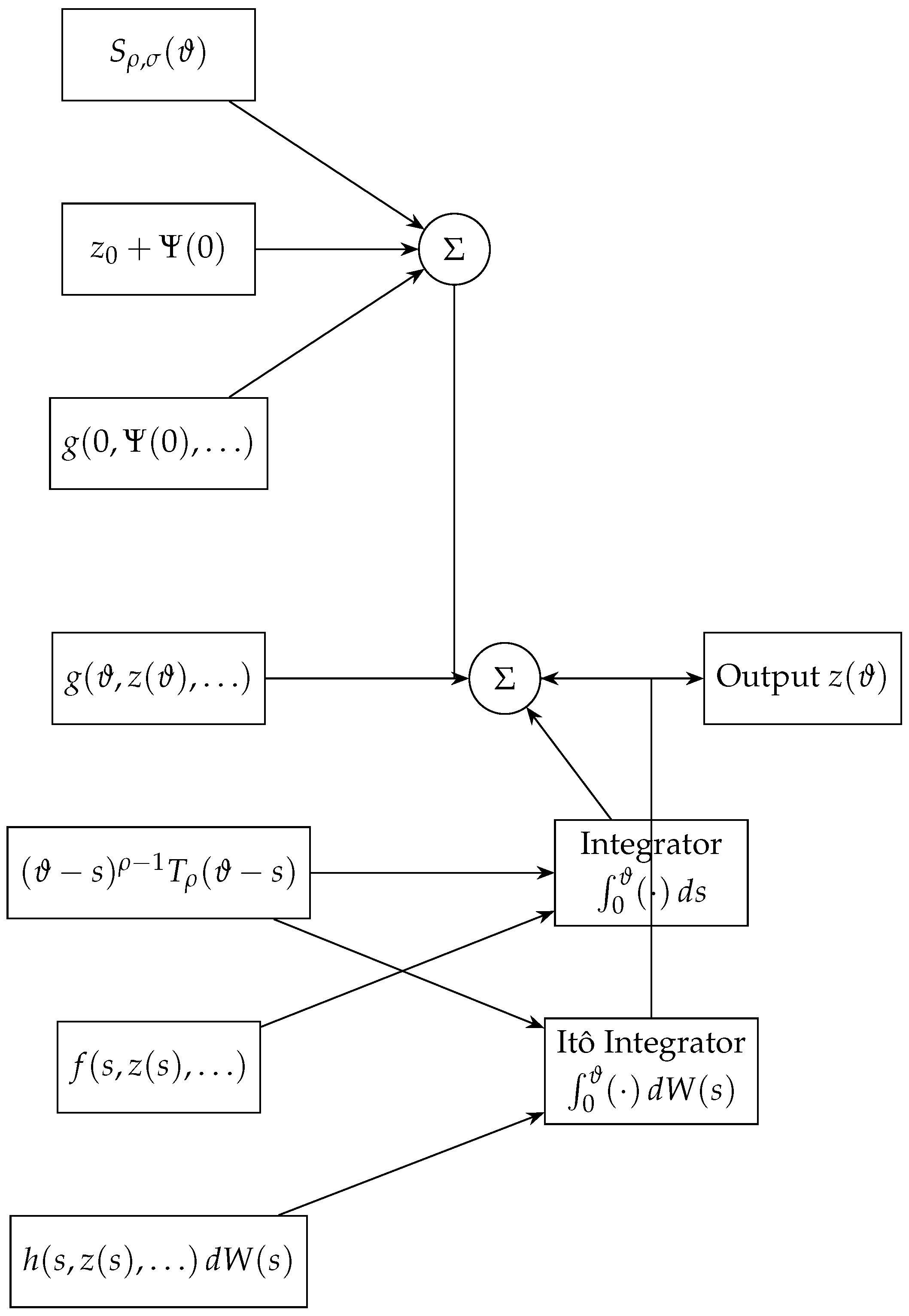
We illustrate the abstract results on a Sobolev-type stochastic filter model generalizing the deterministic filter example of ([7], Section 5). A digital filter processes a sampled input signal to produce an output signal; in practice the input, and hence the filter state, is corrupted by measurement or channel noise, which is naturally modeled as an additive Q-Wiener perturbation acting through the diffusion coefficient h. The system is described symbolically by (1)–(3) with g representing the (delayed) phase-shifting network, f the deterministic Fourier/convolution processing block, and h the noise-injection block; Figure 1 depicts the resulting signal flow. The phase-shifted input $g(\vartheta ,z\left(\vartheta \right),z\left(u_1\left(\vartheta \right)\right),\dots ,z\left(u_p\left(\vartheta \right)\right))$ is combined with the neutral Hilfer fractional memory kernel $S_{\rho ,\sigma }\left(\vartheta \right)$ acting on the nonlocal initial data, the deterministic block ${(\vartheta -s)}^{\rho -1}{T}_{\rho }(\vartheta -s)f$ is integrated against $ds$ over $(0,\vartheta )$, and the stochastic block ${(\vartheta -s)}^{\rho -1}{T}_{\rho }(\vartheta -s)h$ is integrated against the increments $dW\left(s\right)$ of the driving Wiener process; the summer network combines all contributions to output $z\left(\vartheta \right)$.

Taking $\sigma =1$ (Caputo case) and $h\equiv 0$ (no noise) in this model recovers exactly the deterministic filter example of ([7], Section 5), consistent with the reduction noted after Theorem 1.

A Concrete Sobolev-Type Stochastic Heat/Diffusion Example

To make Assumptions 1–7 verifiable in a specific case, consider the spatial domain $\mathcal{O}=(0,\pi )\subset \mathbb{R}$, the Hilbert space $\mathrm{Y}=L^2(0,\pi )$, and the standard eigenbasis ${\chi }_i\left(x\right)=\sqrt{2/\pi }sin\left(ix\right)$, $i=1,2,\dots$, of the Dirichlet Laplacian $-{\partial }_{xx}^2$ on $H^2(0,\pi )\cap H_0^1(0,\pi )$, with eigenvalues $i^2$. Let

$$\mathcal{A}=I-{\partial }_{xx}^2,\mathcal{B}=-{\partial }_{xx}^2,$$

both with domain $H^2(0,\pi )\cap H_0^1(0,\pi )$; these are the classical Sobolev-type operators used, e.g., for pseudo-parabolic (Sobolev, Barenblatt–Zheltov–Kochina) equations, and satisfy (C1)–(C3) with ${\mathcal{A}}^{-1}$ compact and self-adjoint, and with ${\chi }_i$ simultaneously diagonalizing $\mathcal{A},\mathcal{B},\mathcal{E}$ as required by Assumption 1. Then $\mathcal{E}=\mathcal{B}{\mathcal{A}}^{-1}$ has eigenpairs $\left({\alpha }_i,{\chi }_i\right)=\left(i^2/(1+i^2),{\chi }_i\right)$, so $0<{\alpha }_i<1$ for every i and Assumption 1 holds with ${\alpha }_i\uparrow 1$ as $i\to \infty$—a bounded, rather than unbounded, spectrum, which is typical of genuinely Sobolev-type (as opposed to purely parabolic) problems, since (C2) forces $D\left(\mathcal{A}\right)\subset D\left(\mathcal{B}\right)$, which is easiest to arrange when $\mathcal{A},\mathcal{B}$ have comparable order, giving a bounded $\mathcal{E}=\mathcal{B}{\mathcal{A}}^{-1}$. As discussed after Assumption 1, this is deliberately compatible with the Faedo–Galerkin theory of Section 4 (Remark 8), even though the classical spectral-gap rate ${\lambda }_n^{-(\theta -\mu )}\to 0$ does not apply here (since ${\lambda }_n\cancel{\to }\infty$); only the finite-T bound $N_0={sup}_{\vartheta \in [0,T]}∥S\left(\vartheta \right)∥<\infty$ of (4) is used, which holds automatically for this bounded $\mathcal{E}$.

Consider the stochastically forced, delayed, nonlocal Sobolev–Hilfer initial-boundary value problem, for $x\in (0,\pi )$, $\vartheta \in (0,T]$,

$$\begin{array}{cc}\hfill {}^{H}D_{0^{+}}^{\rho ,\sigma }\left[(I-{\partial }_{xx}^2)z(\vartheta ,x)+c_0{\int }_0^{\pi }k(x,\xi )z\left(u_1\left(\vartheta \right),\xi \right)d\xi \right]& =-{\partial }_{xx}^{2}z(\vartheta ,x)+c_{1}sin\left(z(\vartheta ,x)\right)+c_{2}z(\vartheta ,x)\dot{\beta }\left(\vartheta \right),\hfill \\ \hfill z(\vartheta ,0)=z(\vartheta ,\pi )& =0,\vartheta \in [0,T],\hfill \\ \hfill z(\vartheta ,x)& =z_0\left(x\right)+\mathsf{\Psi }(\vartheta ,x),\vartheta \in [-\eta ,0],\hfill \end{array}$$

(43)

with nonlocal condition $I_{0^{+}}^{(1-\rho )(1-\sigma )}\left[(I-{\partial }_{xx}^2)z\right](0^{+},x)+{\sum }_{j=1}^k{c}_j^{\prime }z({\vartheta }_j,x)=(I-{\partial }_{xx}^2)[z_0\left(x\right)+\mathsf{\Psi }(0,x)]$ for fixed $0<{\vartheta }_1<\cdots <{\vartheta }_k\le T$, $k(·,·)\in L^2\left({(0,\pi )}^2\right)$, and $\beta$ a standard real Brownian motion so that $W\left(\vartheta \right)=\beta \left(\vartheta \right)e_0$ (a one-dimensional, hence trivially trace-class, Q-Wiener process with $K=\mathbb{R}$). Here $g_0(\vartheta ,z,z\left(u_1\left(\vartheta \right)\right))=c_0{\int }_0^{\pi }k(·,\xi )z(u_1\left(\vartheta \right),\xi )d\xi =:c_0\mathcal{K}z\left(u_1\left(\vartheta \right)\right)$, $f_0(\vartheta ,z)=c_{1}sin\left(z\right)$, $h_0(\vartheta ,z)=c_{2}z$, ${\phi }_0\left(z\right)={\sum }_j{c}_j^{\prime }z({\vartheta }_j,·)$ are the “physical” maps of (1), and $\mathcal{K}$ denotes the Hilbert–Schmidt integral operator with kernel k.

By Assumption 3, we must verify Assumptions 2–6 for the ${\mathcal{A}}^{-1}$-composed maps $g={\mathcal{A}}^{-1}{g}_0=c_0{\mathcal{A}}^{-1}\mathcal{K}z\left(u_1\left(\vartheta \right)\right)$, $f={\mathcal{A}}^{-1}{f}_0$, $h={\mathcal{A}}^{-1}{h}_0$, $\phi ={\mathcal{A}}^{-1}{\phi }_0$—and, per Assumption 2 (using ${\mathcal{E}}^{\beta }$, as justified in Remark 3), this means verifying that ${\mathcal{E}}^{\beta }g$ (not merely g itself) is Lipschitz. This is straightforward precisely because $\mathcal{E}$ is bounded in this example: ${\mathcal{E}}^{\beta }$ has eigenvalues ${\alpha }_i^{\beta }\in (0,1)$ (bounded by 1, since $0<{\alpha }_i<1$), so $∥{\mathcal{E}}^{\beta }∥\le 1$ on all of $\mathrm{Y}=L^2(0,\pi )$—no domain restriction, and no separate regularity condition on the kernel k beyond $k\in L^2\left({(0,\pi )}^2\right)$ is needed. Since ${\mathcal{A}}^{-1}$ is also bounded ($W_1=∥{\mathcal{A}}^{-1}∥\le 1$, as $1+i^2\ge 1$) and $\mathcal{K}$ is a bounded (Hilbert–Schmidt) operator with $∥\mathcal{K}∥\le {∥k∥}_{L^2\left({(0,\pi )}^2\right)}$,

$${\mathcal{E}}^{\beta }g=c_0{\mathcal{E}}^{\beta }{\mathcal{A}}^{-1}\mathcal{K}z\left(u_1\left(\vartheta \right)\right),\mathbb{E}{∥{\mathcal{E}}^{\beta }g({\vartheta }_1,z_1,\dots )-{\mathcal{E}}^{\beta }g({\vartheta }_2,w_1,\dots )∥}^2\le c_0^2{∥k∥}_{L^2\left({(0,\pi )}^2\right)}^2\mathbb{E}{∥z\left(u_1\left({\vartheta }_1\right)\right)-w\left(u_1\left({\vartheta }_2\right)\right)∥}^2,$$

verifying Assumption 2 for ${\mathcal{E}}^{\beta }g$ (not merely for g) with $L_g\left(r\right)=c_0^2{∥k∥}_{L^2\left({(0,\pi )}^2\right)}^2$, independent of r. As in Remark 3, had we instead tried to hypothesize Lipschitz continuity of ${\mathcal{B}}^{\beta }g$ or ${\mathcal{A}}^{\beta }g$ directly, the argument would fail: $\mathcal{A}=I-{\partial }_{xx}^2$ has eigenvalues $1+i^2\to \infty$, so ${\mathcal{A}}^{\beta }$, and hence ${\mathcal{B}}^{\beta }={\mathcal{E}}^{\beta }{\mathcal{A}}^{\beta }$, is an unbounded operator for every $\beta >0$, and no analogous clean bound would be available. This is precisely why Assumption 2 is phrased in terms of ${\mathcal{E}}^{\beta }$, not ${\mathcal{B}}^{\beta }$. Similarly $f={\mathcal{A}}^{-1}{f}_0$ is bounded ($∥f∥\le W_1{c}_1\sqrt{\pi }$, $W_1=∥{\mathcal{A}}^{-1}∥\le 1$) and globally Lipschitz with constant $\le W_1^2{c}_1^2\le c_1^2$ (since ${\mathcal{A}}^{-1}$ is a contraction here, $∥{\mathcal{A}}^{-1}∥\le 1$, and $|sina-sinb|\le |a-b|$), verifying Assumption 4 with $L_f\left(r\right)\equiv c_1^2$; $h={\mathcal{A}}^{-1}{h}_0$ is linear, hence globally Lipschitz on ${\mathrm{Y}}_{\mu }$ with $L_h\left(r\right)\le c_2^2$, verifying Assumption 5; and $\phi ={\mathcal{A}}^{-1}{\phi }_0={\sum }_{j=1}^k{c}_j^{\prime }{\mathcal{A}}^{-1}z({\vartheta }_j,·)$ is a finite sum of evaluations of the ${\mathrm{Y}}_{\mu }$-valued path $z(·)\in D_T^{\mu }$ at the fixed times ${\vartheta }_j\in [0,T]$, composed with the bounded operator ${\mathcal{A}}^{-1}$—i.e., for each j, $z\mapsto {\mathcal{A}}^{-1}z({\vartheta }_j,·)$ is the (bounded) coordinate map $D_T^{\mu }\to {\mathrm{Y}}_{\mu }$, $z\mapsto z\left({\vartheta }_j\right)$, composed with ${\mathcal{A}}^{-1}$; no spatial embedding is needed (in particular ${\mathrm{Y}}_{\mu }\hookrightarrow C(0,\pi )$ plays no role here, since $\phi$ is not evaluated at a point in space, only in time). Directly from the triangle inequality and $∥{\mathcal{A}}^{-1}∥\le 1$, $\mathbb{E}{∥\phi \left(z_1\right)-\phi \left(z_2\right)∥}_{\mu }^2\le {\left({\sum }_j\left|c_j^{\prime }\right|\right)}^2{sup}_{\vartheta \in [0,T]}\mathbb{E}{∥z_1\left(\vartheta \right)-z_2\left(\vartheta \right)∥}_{\mu }^2$, verifying Assumption 6 with $C_{\phi }={\left({\sum }_j\left|c_j^{\prime }\right|\right)}^2$. Consequently, provided $T,c_0,c_1,c_2,c_j^{\prime }$ are small enough (or T is small enough relative to the fixed $c_0,c_1,c_2,c_j^{\prime }$) that (20) and (21) hold. Because all the Lipschitz constants above are global (independent of r), the conditions reduce here to a single explicit smallness inequality in T, whose right-hand side involves only $\rho ,\mu ,\beta ,\sigma ,T$ and the coefficients $c_0,c_1,c_2,c_j^{\prime }$, all of which are freely at the experimenter’s disposal.

Remark 9 

(An explicit admissible parameter choice). Take $\rho =0.9$, $\mu =0.3$, $\beta =0.1$, $\sigma =1$ as in Remark 1, so that $\rho (1-\mu )=0.63>1/2$; a single delay term ($p=1$) with $u_1\left(\vartheta \right)=q\vartheta$, $0\le q\le 1$ (e.g., $q=1/2$), which satisfies Assumption 7; a single nonlocal evaluation time $k=1$, ${\vartheta }_1=T/2$; and coefficients $c_0=c_1=c_2=c_1^{\prime }=0.05$, together with a horizon $T=0.1$. With this choice every Lipschitz/growth constant appearing in (20) and (21) above is proportional to $c_0^2,c_1^2,c_2^2$, or ${\left(c_1^{\prime }\right)}^2$, i.e., to $0.0025$, while the various Gamma-function and T-power prefactors in (20) and (21) are, for these values of $\rho ,\mu ,\beta$ and $T=0.1$, all of moderate size (none of the relevant exponents $2\rho (1-\mu )-1=0.134$, $2\rho (\mu -\beta )=0.36$ is close to a Gamma-function pole); consequently the left-hand sides of (20) and (21) are of order $c^2\times T^{(\mathit{small}\mathit{positive}\mathit{power})}\ll 1$ for $c=0.05$, and (20) and (21) hold for this choice (and, by continuity, for an open neighborhood of it) with substantial room to spare, e.g., by taking $R=1$ once $\mathbb{E}{∥z_0+\mathsf{\Psi }\left(0\right)∥}_{\mu }^2$ and $\mathbb{E}{∥\mathsf{\Psi }∥}_{0,\mu }^2$ are also fixed at order-1 values. This confirms concretely, rather than only qualitatively, that problem (43) satisfies the hypotheses of Theorems 1, 4, and 5.

Theorem 1 guarantees problem (43) has a unique mild solution $z\in B_R(D_T^{\mu },\tilde{\mathsf{\Psi }})$, Theorem 4 guarantees the fixed point iterates $z_n$ converge to it in mean square, and Theorem 5 guarantees that its truncated Fourier (Galerkin) approximations ${\overline{z}}_n(\vartheta ,x)={\sum }_{i=1}^n{\rho }_i^n\left(\vartheta \right){\chi }_i\left(x\right)$, obtained by numerically solving the coupled scalar system (42)—here, a system of n coupled real-valued Hilfer stochastic fractional differential equations driven by the single Brownian motion $\beta$—converge to z in mean square as $n\to \infty$. This example also illustrates the role of $\sigma$: taking $\sigma \to 1$ makes the nonlocal condition above converge to the Caputo-type pointwise condition $(I-{\partial }_{xx}^2)z(0,x)+{\sum }_j{c}_j^{\prime }z({\vartheta }_j,x)=(I-{\partial }_{xx}^2)[z_0\left(x\right)+\mathsf{\Psi }(0,x)]$, whereas $\sigma <1$ allows the initial datum to be prescribed only on a fractional integral (i.e., a time-averaged, memory-weighted version) of the neutral term, which is the physically relevant choice whenever the “initial” measurement of the system is itself obtained through an averaging or filtering process, as is common in the digital-filter interpretation of Figure 1. In terms of the underlying filter, $c_0$ scales the strength of the delayed feedback/memory coupling encoded by the kernel k, $c_1$ scales the (saturating, since $|sin|\le 1$) nonlinear forcing intrinsic to the filter dynamics, and $c_2$ scales the intensity of the additive channel or measurement noise; the smallness condition of Remark 9 therefore has the concrete reading that a stable, uniquely solvable filter model of this Sobolev type is guaranteed whenever the feedback strength, nonlinearity, and noise intensity are jointly moderate relative to the observation horizon T, which is the regime of practical interest for a lightly damped digital filter. The advantage of the Hilfer derivative over the Caputo derivative in this model is precisely the extra type parameter $\sigma$ just discussed: a purely Caputo-based model ($\sigma =1$ in our formulation) forces the nonlocal/initial condition to be a pointwise statement about $z(0,·)$ itself, whereas a filter whose very first reading is already an average over a short warm-up window—for instance, a running-average or low-pass pre-filter applied before sampling begins—is more faithfully modeled by $\sigma <1$, where the initial data constrains only $I_{0^{+}}^{(1-\rho )(1-\sigma )}[·]\left(0^{+}\right)$, a fractional-integral (memory-weighted) functional of the neutral term rather than its instantaneous value; the Hilfer formulation therefore strictly enlarges, rather than merely generalizes for its own sake, the class of physically realizable initial measurements this model can represent.

6. Conclusions

We generalized the neutral, nonlocal, Sobolev-type fractional differential equation with finite delay of Kaliraj et al. [7] in two independent directions: replacing the Caputo derivative by the more general Hilfer fractional derivative ^H$D_{0^{+}}^{\rho ,\sigma }$, and adding a stochastic perturbation driven by a Q-Wiener process. Using a probability-density (Mainardi–Wright) representation of the associated Hilfer semigroup-type operators $S_{\rho ,\sigma }\left(\vartheta \right)$ and $T_{\rho }\left(\vartheta \right)$, we derived the stochastic Volterra mild-solution formula, established existence and uniqueness of the mild solution in the mean-square sense via the Banach contraction principle, and constructed a Faedo–Galerkin approximation scheme whose solutions converge in mean square to the unique mild solution. Setting $\sigma =1$ and $h\equiv 0$ recovers precisely the results of [7], confirming the present work as a strict generalization; we also established, as a genuinely new result with no counterpart in [7], mean-square continuous dependence of the mild solution on the nonlocal and delay data (Theorem 2), and verified the full set of hypotheses on a concrete Sobolev-type stochastic heat/diffusion example with a finite-delay nonlocal condition (Section The Faedo–Galerkin Scheme).

Several directions remain open for future work.

(a)

Local, rather than global, Lipschitz hypotheses. Assumptions 2–6 are global (or, in the case of $L_g,L_f,L_h$, uniform over bounded sets with the ball radius r fixed in advance); a genuinely local theory, in which the Lipschitz constants are allowed to blow up as $r\to \infty$ and existence is obtained on a possibly shrinking time interval via a standard continuation/truncation argument, would substantially broaden the class of nonlinearities $g,f,h$ covered, at the cost of a more delicate analysis of the maximal interval of existence.

(b)

Approximate controllability. A natural next step, in the spirit of [13,24,25,26,27], is to append a control term $\mathcal{C}u\left(\vartheta \right)$ (with $\mathcal{C}$ a bounded linear control operator and u taking values in a separable control Hilbert space U) to the right-hand side of (1) and to study approximate controllability of the resulting Hilfer stochastic Sobolev-type neutral system with finite delay, using the associated controllability (Gramian) operator together with the fixed point and Faedo–Galerkin machinery developed here.

(c)

Impulsive effects. Finally, combining the present framework with instantaneous or non-instantaneous impulses at the switching times ${\vartheta }_k$ already present in the weighted space $D_T^{\mu }$ (but not otherwise used in the Equation (1) itself) would connect this work back to the impulsive Sobolev-type Caputo theory of [8] and its references, now in the Hilfer stochastic setting.

(d)

Infinite delay and other driving noises. The finite delay hypothesis (Assumption 7) could be relaxed to infinite delay via a suitable phase space, in the spirit of [14,15]; combined with the present Sobolev-type, finite-delay, Faedo–Galerkin machinery, this would remove one of the few remaining gaps relative to the existing Hilfer stochastic literature discussed in Section 1. Likewise, replacing the Q-Wiener process W by fractional Brownian motion or a Rosenblatt process, as in [18], would connect the present results to the growing literature on non-Markovian driving noise for Hilfer fractional systems.

(e)

Numerical validation. The coordinate system (42) underlying the Faedo–Galerkin scheme is, by construction, amenable to numerical simulation via a fractional Euler–Maruyama or similar scheme; a systematic numerical study of the convergence rate of ${\overline{z}}_n$ to z (complementing the qualitative convergence established in Theorem 5 and the rate discussion of Remark 8) on the concrete filtering model of Section 5 is a natural and, we expect, tractable next step.

Taken together, these directions would extend the present theory of existence, uniqueness, and approximation toward the controllability, long-time behavior, and computational questions that are of most direct interest in the filtering applications that motivate the Sobolev-type model of Section 5.

References

1. Khan, W.A.; Wani, S.A.; Ayman-Mursaleen, M.; Kotecha, K.; Jadhav, P. Extended forms of Legendre-Laguerre-based hybrid polynomials and their characteristics via fractional operator approach. J. Inequal. Appl. 2026, 2026, 24. [Google Scholar] [CrossRef] [Scilit]
2. Riyasat, M.; Wani, S.A.; Khan, S.; Shah, S. Operational perspective on degenerate Gould–Hopper–Fubini polynomials using fractional calculus. Georgian Math. J. 2026. [Google Scholar] [CrossRef] [Scilit]
3. Hilfer, R. (Ed.) Applications of Fractional Calculus in Physics; World Scientific: Singapore, 2000. [Google Scholar]
4. Furati, K.M.; Kassim, M.D.; Tatar, N.E. Existence and uniqueness for a problem involving Hilfer fractional derivative. Comput. Math. Appl. 2012, 64, 1616–1626. [Google Scholar] [CrossRef] [Scilit]
5. Gu, H.; Trujillo, J.J. Existence of mild solution for evolution equation with Hilfer fractional derivative. Appl. Math. Comput. 2015, 257, 344–354. [Google Scholar] [CrossRef] [Scilit]
6. Debbouche, A.; Nieto, J.J. Sobolev type fractional abstract evolution equations with nonlocal conditions and optimal multi-controls. Appl. Math. Comput. 2014, 245, 74–85. [Google Scholar] [CrossRef] [Scilit]
7. Kaliraj, K.; Manjula, M.; Thilakraj, E.; Ravichandran, C.; Nisar, K.S.; El-Ebiary, Y.A.B.; Hourani, A.O. Discussions on Sobolev type Neutral Nonlocal fractional differential equation. Partial Differ. Equ. Appl. Math. 2025, 13, 101018. [Google Scholar] [CrossRef] [Scilit]
8. Kaliraj, K.; Manjula, M.; Ravichandran, C.; Nisar, K.S. Results on neutral differential equation of sobolev type with nonlocal conditions. Chaos Solitons Fractals 2022, 158, 112060. [Google Scholar] [CrossRef] [Scilit]
9. Prato, G.D.; Zabczyk, J. Stochastic Equations in Infinite Dimensions; Cambridge University Press: Cambridge, UK, 1992. [Google Scholar]
10. Byszewski, L. Theorems about the existence and uniqueness of solutions of a semilinear evolution nonlocal Cauchy problem. J. Math. Anal. Appl. 1991, 162, 497–505. [Google Scholar] [CrossRef] [Scilit]
11. Zhou, Y.; Jiao, F. Nonlocal Cauchy problem for fractional evolution equations. Nonlinear Anal. Real World Appl. 2010, 11, 4465–4475. [Google Scholar] [CrossRef] [Scilit]
12. Mao, X. Stochastic Differential Equations and Applications, 2nd ed.; Horwood Publishing: Chichester, UK, 2007. [Google Scholar]
13. Sakthivel, R.; Ren, Y.; Mahmudov, N.I. On the approximate controllability of semilinear fractional differential systems. Comput. Math. Appl. 2011, 62, 1451–1459. [Google Scholar] [CrossRef] [Scilit]
14. Pradeesh, J.; Vijayakumar, V. On the Asymptotic Stability of Hilfer Fractional Neutral Stochastic Differential Systems with Infinite Delay. Qual. Theory Dyn. Syst. 2024, 23, 153. [Google Scholar] [CrossRef] [Scilit]
15. Sivasankar, S.; Udhayakumar, R.; Muthukumaran, V.; Gokul, G.; Al-Omari, S. Existence of Hilfer fractional neutral stochastic differential systems with infinite delay. Bull. Karaganda Univ. Math. Ser. 2024, 113, 174–193. [Google Scholar] [CrossRef] [Scilit]
16. Shah, R.; Irshad, N. Existence and uniqueness of solutions of Hilfer fractional neutral impulsive stochastic delayed differential equations with nonlocal conditions. J. Nonlinear Complex Data Sci. 2026, 27, 43–63. [Google Scholar] [CrossRef] [Scilit]
17. Raheem, A.; Alamrani, F.M.; Akhtar, J.; Alatawi, A.; Alshaban, E.; Khatoon, A.; Khan, F.A. Study on Controllability for Ψ-Hilfer Fractional Stochastic Differential Equations. Fractal Fract. 2024, 8, 727. [Google Scholar] [CrossRef] [Scilit]
18. Lavanya, M.; Vadivoo, B.S.; Nisar, K.S. Controllability Analysis of Neutral Stochastic Differential Equation Using Ψ-Hilfer Fractional Derivative With Rosenblatt Process. Qual. Theory Dyn. Syst. 2025, 24, 19. [Google Scholar] [CrossRef] [Scilit]
19. Lv, J.; Yang, M. A Study Concerning to the Existence and Averaging Principle for Ψ-Hilfer Fractional Stochastic Evolution Equations. Math. Methods Appl. Sci. 2025, 48, 15773–15783. [Google Scholar] [CrossRef] [Scilit]
20. Dhanush, A.; Vijayakumar, V. Results on the existence and time optimal control results for Hilfer fractional stochastic differential inclusions in Hilbert spaces. J. Appl. Math. Comput. 2025, 71, 3997–4023. [Google Scholar] [CrossRef] [Scilit]
21. Gou, H. Study on Sobolev type Hilfer evolution equations with non-instantaneous impulses. Int. J. Comput. Math. 2023, 100, 1153–1170. [Google Scholar] [CrossRef] [Scilit]
22. Gou, H.; Li, Y. Extremal mild solutions to Hilfer evolution equations with non-instantaneous impulses and nonlocal conditions. Fract. Calc. Appl. Anal. 2023, 26, 1145–1185. [Google Scholar] [CrossRef] [Scilit]
23. Pazy, A. Semigroups of Linear Operators and Applications to Partial Differential Equations; Applied Mathematical Sciences; Springer: New York, NY, USA, 1983; p. 44. [Google Scholar]
24. Ayman-Mursaleen, M.; Alshaban, E.; Nasiruzzaman, M. Approximation to family of α-Bernstein operators using shifted knot properties. J. Inequal. Appl. 2025, 2025, 107. [Google Scholar] [CrossRef] [Scilit]
25. Ayman-Mursaleen, M. Controllability of tempered Caputo fractional dynamical systems. J. Nonlinear Convex Anal. 2025, 26, 2501–2511. [Google Scholar]
26. Haque, I. Controllability for Ψ-Hilfer fractional Sobolev-type stochastic differential system. Fixed Point Theory Algorithms Sci. Eng. 2026, 2026, 27. [Google Scholar] [CrossRef] [Scilit]
27. Ayman-Mursaleen, M.; Saeed, S.; Almohammadi, S.; Arif, K.; Imran, M. A deep neural network model for heat transfer in darcy–forchheimer hybrid nanofluid flow with activation energy. Sci. Rep. 2026, 16, 8339. [Google Scholar] [CrossRef] [Scilit] [PubMed]
Figure 1. Signal-flow diagram of the stochastically perturbed Sobolev-type Hilfer filter model. The deterministic Fourier/convolution path (f, ordinary integrator) and the noise-injection path (h, Itô integrator) are combined at the summer network together with the neutral memory term g and the nonlocal/initial contribution processed by S ρ , σ ( ϑ ) .
Fractalfract 10 00652 g001