Article

Solvability of Nonlinear Discrete Fractional Equations with Mixed-Order Nabla Operators and Dirichlet Boundaries

by
Nikolay D. Dimitrov
1,*,† and
Jagan Mohan Jonnalagadda
2,†
1
Department of Mathematics, University of Ruse, 7017 Ruse, Bulgaria
2
Department of Mathematics, Birla Institute of Technology and Science Pilani, Hyderabad 500078, India
*
Author to whom correspondence should be addressed.
These authors contributed equally to this work.
Fractal Fract. 2026, 10(9), 641; https://doi.org/10.3390/fractalfract10090641
Submission received: 29 July 2026 / Revised: 9 September 2026 / Accepted: 12 September 2026 / Published: 14 September 2026
(This article belongs to the Special Issue Advances in Fractional Initial and Boundary Value Problems)

Abstract

In this manuscript, we study the solvability of a class of mixed-order nabla fractional equations coupled with Dirichlet conditions. Based on the obtained Green’s function and its properties, we establish existence, nonexistence, and multiplicity results using fixed point theory. In the end, we give some numerical examples that verify our theoretical results.

1. Introduction

Over the last few decades, research has clearly shown that fractional-order models outperform integer-order models in terms of accuracy. For example, fractional-order models in epidemiology have been shown to replicate real-world epidemic data more accurately than classical models [1,2,3,4]. This has led to a significant increase in research on such problems in the delta [5,6,7,8] and nabla [9,10,11,12] cases using Riemann–Liouville or Caputo operators. The main framework of nabla fractional calculus was introduced in earlier works such as [13,14,15], where fundamental definitions and basic properties of fractional sums and differences were given. This framework has since been significantly expanded with many new results driven by a wide range of real-world applications in scientific and technical fields, including modeling systems based on discrete data in economics, biology, and physics as well as in signal processing and control theory [16,17,18,19,20,21]. For a comprehensive introduction to the fundamental aspects of this topic, we refer the reader to the monographs [22,23,24,25] and the references therein. Recently, there has been a significant increase in the study of nabla problems, as they allow for more reliable modeling of long-term memory effects [26,27,28,29], making them particularly suitable for describing processes that are nonlocal in time or space. Based on different arguments, existence results have been obtained recently; however, almost all of these studies deal with nabla models with one fractional operator.
Such results exist for fractional boundary value problem; for example, in ref [30], Graef et. al. obtained existence results for
D 0 + α ω ( t ) + a D 0 + β ω ( t ) = w ( t ) f ω ( t ) , 0 β < 1 < α < 2 , a R , 0 < t < 1 .
Later, these results were extended in [31,32,33].
As we mentioned before, there are only three papers in the existing literature which have considered a nabla fractional problem with more than one Riemann–Liouville operator [34,35,36]; however, in all of these the second nabla operator was in the boundary conditions. In detail, in all of the above mentioned works, the following nabla problem was considered:
ρ ( ι ) ζ ω ( κ ) = J ( κ , ω ( κ ) ) , κ N ι + 2 b
coupled to Neumann-type conditions
ω ( ι ) = ρ ( ι ) ϑ ω ( b ) = 0 ,
to summation conditions in the form
ω ( ι ) = 0 , ρ ( ι ) ϑ ω ( b ) = α s = ι + 1 d ω ( s ) , d N ι + 1 b 1 , α > 0 ,
and to three-point conditions
ω ( ι ) = 0 , ρ ( ι ) ϑ ω ( b ) = α ρ ( ι ) ϑ ω ( ξ ) , ξ N ι + 1 b 1 , 0 < α 1 ,
respectively. Here, 0 ϑ 1 < ζ < 2 . With the idea of filling this gap in the existing literature, and inspired by recent works [37,38] where such problems have been studied for the discrete delta fractional case
Δ ζ ω ( κ ) + α Δ ϑ ω ( κ + ζ ϑ 1 ) = J ( κ + ζ ϑ 1 ) κ [ 0 , b + 1 ] N 0
coupled to Dirichlet conditions (where α R and 0 < ϑ < 1 < ζ < 2 ), in this manuscript we consider the following problem.

Formulation of the Problem

ρ ( ι ) ζ ω ( κ ) + Λ ρ ( ι ) ϑ ω ( κ ) = J ( κ , ω ( κ ) ) , κ N ι + 2 b
ω ( ι ) = ω ( b ) = 0
Here, 0 < ϑ < 1 < ζ < 2 , 1 < Λ < 1 , and J : N ι + 2 b × R R . With these assumptions, we construct the Green’s function corresponding to the considered problem consisting of (1) and (2) (Theorem 4). Further, we suppose that 1 < 1 + ϑ ζ < 2 and Λ 0 , Λ * in order to show that the Green’s function is non-negative on its domain of definition (Theorem 5).
Note that for our problem, as for any other that deals with two different fractional terms, there are clear real-world physical application. As shown in [39,40], the first term of order 1 < ζ < 2 shows fractional inertia, while the second term of order 0 < ϑ < 1 shows fractional damping with long memory. In detail, fractional inertia is a property of a system in which the force acceleration relation depends on a power-law weighted history of past motion, leading to a fractional derivative of order between 1 and 2 in Newton’s law, as in the considered problem (1). Fractional damping is a memory-dependent dissipation mechanism in which the damping force is proportional to a fractional derivative of displacement (order between 0 and 1, as in problem (1)), which means that it depends on a power-law weighted history of past velocities rather than only the instantaneous velocity.
We point out that in the classical beam equation ω + Λ ω , fixed at both ends with Dirichlet conditions, the first term represents acceleration, while the second gives viscous damping. In this classical model, the acceleration depends only on the present state and the damping depends only on the present velocity. The material has no long-term memory and the system “forgets” its past exponentially fast. It is experimentally proven that this model works well for ideal fluids, but fails when dealing with complex materials. Real materials such as polymers, biological tissues, composite materials, and porous media display long memory and cannot be modeled without fractional models.
In other words, while the classical equation assumes instantaneous damping and inertia, the considered problem in (1) and (2) captures the distributed memory effects observed in real complex materials, providing a more accurate and physically realistic representation. Thus, the problem that we consider models a fixed viscoelastic structure made of a complex material in which inertia and damping both depend on the entire history of motion, producing realistic long-memory vibration behavior such as observed in polymers, composites, and biological tissues.
This work is structured as follows: in Section 2, we recall the definition and some well-known properties of the nabla Mittag–Leffler function that are used in the present manuscript; Section 3 and Section 4 are devoted to the construction of the related Green’s function to the linear problem and to establishing some very useful bounds on it, respectively; in Section 5, under suitable conditions of nonlinearity, we present different uniqueness, existence, nonexistence, and multiplicity results for the considered problem using fixed point theory; at the end of the paper, Section 6 provides some examples that demonstrate the applications of our theoretical findings, while in Section 7 we discuss how the novel idea of this paper can be extended in future work.
To the best of our knowledge, a mixed-order nabla fractional problem has not previously been investigated in the literature. We point out that we consider the main mathematical novelty of this work to lie in constructing the Green’s function and deducing some of its useful properties. In detail, we investigate a previously unexplored mixed-order nabla fractional operator coupled to Dirichlet boundary conditions. The main contribution is the derivation and analysis of the corresponding Green’s function, which cannot be obtained by directly adapting the Green’s function of a single-order fractional problem. The interaction between the two different fractional orders fundamentally changes both the associated linear operator and its inverse, since the mixed operator has a different kernel from either of its individual components. Therefore, finding the exact expression of the Green’s function and establishing its qualitative properties provides the essential foundation for deriving the summation formulation and applying fixed point theory to obtain new uniqueness, existence, and multiplicity results for the nonlinear problem. Moreover, this novel idea can be extended to different higher-order fractional problems or nonlinear systems coupled to different boundary conditions.

2. Preliminaries

To the end of this work, we use the notation and definitions given in [24]. Represent by N ϰ = { ϰ , ϰ + 1 , ϰ + 2 , } , N ϰ f = { ϰ , ϰ + 1 , ϰ + 2 , , f } for any real ϰ and f with f ϰ N 1 .
For the reader’s convenience, we recall some basic definitions and properties of nabla fractional operators and Mittag–Leffler functions.
Definition 1
([24]). The rising function is
a b ¯ = Γ ( a + b ) Γ ( a )
for any a, b R .
Definition 2
([24]). Let β be any real number except the negative integer. The β t h nabla fractional Taylor monomial is
H β ( ζ , k ) = ( ζ k ) β ¯ Γ ( β + 1 ) .
Lemma 1
([10,24]). Let ς N l and υ > 1 :
(a) 
H υ ( ζ , ς 1 ) 0 , ζ N ς 1 ; H υ ( ζ , ς 1 ) > 0 , ζ N ς ;
(b) 
H υ ( ζ , ς 1 ) decreases with respect to ς for ζ N ς 1 and υ > 0 . Moreover, it increases with respect to ζ for ζ N ς and υ > 0 ;
(c) 
H υ ( ζ , l ) H υ 1 ( ζ , l ) = H υ ( ζ , l + 1 ) .
Definition 3
([24]). Let α, β, λ R such that α > 0 and 1 < λ < 1 . The nabla Mittag–Leffler function is defined by
E λ , α , β ( t , a ) = n = 0 λ n H α n + β ( t , a ) , t N a .
Lemma 2
([24]). Let α, β, λ, ν R such that α, υ > 0 , 1 < λ < 1 , and choose N N 1 such that N 1 < ν N . Then,
1. 
E λ , α , β ( t , ρ ( t ) ) = 1 1 λ , t N a ;
2. 
ρ ( a ) ν E λ , α , β ( t , ρ ( a ) ) = E λ , α , β ν ( t , ρ ( a ) ) , t N a + N ;
3. 
ρ ( a ) ν E λ , ν , ν 1 ( t , ρ ( a ) ) = λ E λ , ν , ν 1 ( t , ρ ( a ) ) , t N a + N ;
4. 
ρ ( a ) ν E λ , ν , ν 2 ( t , ρ ( a ) ) = λ E λ , ν , ν 2 ( t , ρ ( a ) ) , t N a + N .
Our main tool is the Guo–Krasnosel’skii theorem in cones [41].
Theorem 1.
Let B = B , · be a Banach space and let K B be a cone. Assume that Ω 1 and Ω 2 are bounded open subsets contained in B such that 0   Ω 1 and Ω 1   Ω 2 . Assume further that T : K Ω 2 ¯ Ω 1 K is a completely continuous operator. If either:
(1) 
T y y for y K Ω 1 and T y y for y K Ω 2 , or
(2) 
T y y for y K Ω 1 and T y y for y K Ω 2 ,
then T has at least one fixed point in K Ω 2 ¯ Ω 1 .

3. Construction of Green’s Function

The aim of this section is to construct the Green’s function for the linear boundary value problem
ρ ( ι ) ζ ω ( κ ) + Λ ρ ( ι ) ϑ ω ( κ ) = h ( κ ) , κ N ι + 2 b ,
with Dirichlet conditions (2). Here, 0 < ϑ < 1 < ζ < 2 , 1 < Λ < 1 , and h : N ι + 2 b R .
We use the standard notation for the nabla Mittag–Leffler function:
E Λ , ζ , ϑ ( κ , ι ) = n = 0 Λ n H ζ n + ϑ ( κ , ι ) , κ N ι .
Theorem 2.
The general solution of
ρ ( ι ) ζ ω ( κ ) + Λ ρ ( ι ) ϑ ω ( κ ) = 0 , κ N ι + 2
can be expressed as
ω ( κ ) = C 1 E Λ , ζ ϑ , ζ 1 ( κ , ρ ( ι ) ) + C 2 E Λ , ζ ϑ , ζ 2 ( κ , ρ ( ι ) ) , κ N ι ,
with C 1 and C 2 being some arbitrary constants.
Proof. 
For κ N ι + 2 ,
ρ ( ι ) ζ E Λ , ζ ϑ , ζ 1 ( κ , ρ ( ι ) ) + Λ ρ ( ι ) ϑ E Λ , ζ ϑ , ζ 1 ( κ , ρ ( ι ) ) = Λ E Λ , ζ ϑ , ζ ϑ 1 ( κ , ρ ( ι ) ) + Λ E Λ , ζ ϑ , ζ ϑ 1 ( κ , ρ ( ι ) ) = 0 .
Moreover, one can verify
ρ ( ι ) ζ E Λ , ζ ϑ , ζ 2 ( κ , ρ ( ι ) ) + Λ ρ ( ι ) ϑ E Λ , ζ ϑ , ζ 2 ( κ , ρ ( ι ) ) = Λ E Λ , ζ ϑ , ζ ϑ 2 ( κ , ρ ( ι ) ) + Λ E Λ , ζ ϑ , ζ ϑ 2 ( κ , ρ ( ι ) ) = 0 .
Thus, E Λ , ζ ϑ , ζ 1 ( κ , ρ ( ι ) ) and E Λ , ζ ϑ , ζ 2 ( κ , ρ ( ι ) ) are solutions of (4) on N ι . Clearly, they are independent on N ι . □
Theorem 3.
Let h : N ι + 2 b R . The general solution of the linear problem
ρ ( ι ) ζ ω ( κ ) + Λ ρ ( ι ) ϑ ω ( κ ) = h ( κ ) , κ N ι + 2
can be written in the form
ω ( κ ) = C 1 E Λ , ζ ϑ , ζ 1 ( κ , ρ ( ι ) ) + C 2 E Λ , ζ ϑ , ζ 2 ( κ , ρ ( ι ) ) s = ι + 1 κ E Λ , ζ ϑ , ζ 1 ( κ , ρ ( s ) ) h ( s ) , κ N ι
for arbitrary constants C 1 and C 2 .
Proof. 
For κ N ι , set
v ( κ ) = s = ι + 1 κ E Λ , ζ ϑ , ζ 1 ( κ , ρ ( s ) ) h ( s ) .
In view of Theorem 2, it is enough to verify
ρ ( ι ) ζ v ( κ ) + Λ ρ ( ι ) ϑ v ( κ ) = h ( κ ) , κ N ι + 2 b .
Notice that for κ N ι we have
s = ι + 1 κ E Λ , ζ ϑ , ζ 1 ( κ , ρ ( s ) ) h ( s ) = s = ι + 1 κ n = 0 Λ n H ( ζ ϑ ) n + ( ζ 1 ) ( κ , ρ ( s ) ) h ( s ) = n = 0 Λ n s = ι + 1 κ H ( ζ ϑ ) n + ( ζ 1 ) ( κ , ρ ( s ) ) h ( s ) = n = 0 Λ n s = ι κ H ( ζ ϑ ) n + ( ζ 1 ) ( κ , ρ ( s ) ) h ( s ) H ( ζ ϑ ) n + ( ζ 1 ) ( κ , ρ ( ι ) ) h ( ι ) = n = 0 Λ n ρ ( ι ) ( ζ ϑ ) n + ζ h ( κ ) H ( ζ ϑ ) n + ( ζ 1 ) ( κ , ρ ( ι ) ) h ( ι ) = n = 0 Λ n ρ ( ι ) ( ζ ϑ ) n + ζ h ( κ ) E Λ , ζ ϑ , ζ 1 ( κ , ρ ( ι ) ) h ( ι ) .
Thus, for κ N ι + 2 we obtain
ρ ( ι ) ζ v ( κ ) + Λ ρ ( ι ) ϑ v ( κ ) = n = 0 Λ n ρ ( ι ) ζ ρ ( ι ) ( ζ ϑ ) n + ζ h ( κ ) ρ ( ι ) ζ E Λ , ζ ϑ , ζ 1 ( κ , ρ ( ι ) ) h ( ι ) Λ n = 0 Λ n ρ ( ι ) ϑ ρ ( ι ) ( ζ ϑ ) n + ζ h ( κ ) + Λ ρ ( ι ) ϑ E Λ , ζ ϑ , ζ 1 ( κ , ρ ( ι ) ) h ( ι ) = n = 0 Λ n ρ ( ι ) ( ζ ϑ ) n h ( κ ) Λ E Λ , ζ ϑ , ζ ϑ 1 ( κ , ρ ( ι ) ) h ( ι ) Λ n = 0 Λ n ρ ( ι ) ( ζ ϑ ) ( n + 1 ) h ( κ ) + Λ E Λ , ζ ϑ , ζ ϑ 1 ( κ , ρ ( ι ) ) h ( ι ) = h ( κ ) + n = 1 Λ n ρ ( ι ) ( ζ ϑ ) n h ( κ ) Λ n = 0 Λ n ρ ( ι ) ( ζ ϑ ) ( n + 1 ) h ( κ ) = h ( κ ) + Λ n = 0 Λ n ρ ( ι ) ( ζ ϑ ) ( n + 1 ) h ( κ ) Λ n = 0 Λ n ρ ( ι ) ( ζ ϑ ) ( n + 1 ) h ( κ ) = h ( κ ) ,
implying that (8) holds. The proof is complete. □
Theorem 4.
The linear nabla fractional problem (3)–(2) has a unique solution
ω ( κ ) = s = ι + 2 b R ( κ , s ) h ( s ) , κ N ι b ,
where
R ( κ , s ) = R 1 ( κ , s ) , κ N ι ρ ( s ) , R 2 ( κ , s ) , κ N s b
with
R 1 ( κ , s ) = E Λ , ζ ϑ , ζ 1 ( κ , ι ) E Λ , ζ ϑ , ζ 1 ( b , ρ ( s ) ) E Λ , ζ ϑ , ζ 1 ( b , ι )
and
R 2 ( κ , s ) = E Λ , ζ ϑ , ζ 1 ( κ , ι ) E Λ , ζ ϑ , ζ 1 ( b , ρ ( s ) ) E Λ , ζ ϑ , ζ 1 ( b , ι ) E Λ , ζ ϑ , ζ 1 ( κ , ρ ( s ) ) .
Proof. 
From (7) and the first boundary condition ω ( ι ) = 0 , we get
C 1 + C 2 = 0 .
Next, from (7) and ω ( b ) = 0 we deduce
C 1 E Λ , ζ ϑ , ζ 1 ( b , ρ ( ι ) ) + C 2 E Λ , ζ ϑ , ζ 2 ( b , ρ ( ι ) ) s = ι + 1 b E Λ , ζ ϑ , ζ 1 ( b , ρ ( s ) ) h ( s ) = 0 .
Using (13) in (14), we obtain
C 1 E Λ , ζ ϑ , ζ 1 ( b , ρ ( ι ) ) E Λ , ζ ϑ , ζ 2 ( b , ρ ( ι ) ) s = ι + 1 b E Λ , ζ ϑ , ζ 1 ( b , ρ ( s ) ) h ( s ) = 0 .
Since
E Λ , ζ ϑ , ζ 1 ( b , ρ ( ι ) ) E Λ , ζ ϑ , ζ 2 ( b , ρ ( ι ) ) = n = 0 Λ n H ( ζ ϑ ) n + ( ζ 1 ) ( b , ρ ( ι ) ) n = 0 Λ n H ( ζ ϑ ) n + ( ζ 2 ) ( b , ρ ( ι ) ) = n = 0 Λ n H ( ζ ϑ ) n + ( ζ 1 ) ( b , ρ ( ι ) ) H ( ζ ϑ ) n + ( ζ 2 ) ( b , ρ ( ι ) ) = n = 0 Λ n H ( ζ ϑ ) n + ( ζ 1 ) ( b , ι ) = E Λ , ζ ϑ , ζ 1 ( b , ι ) ,
from (15) we can compute
C 1 = 1 E Λ , ζ ϑ , ζ 1 ( b , ι ) s = ι + 1 b E Λ , ζ ϑ , ζ 1 ( b , ρ ( s ) ) h ( s )
and
C 2 = C 1 = 1 E Λ , ζ ϑ , ζ 1 ( b , ι ) s = ι + 1 b E Λ , ζ ϑ , ζ 1 ( b , ρ ( s ) ) h ( s ) .
Using (16) and (17) in (7), we obtain
ω ( κ ) = E Λ , ζ ϑ , ζ 1 ( κ , ι ) E Λ , ζ ϑ , ζ 1 ( b , ι ) s = ι + 1 b E Λ , ζ ϑ , ζ 1 ( b , ρ ( s ) ) h ( s ) s = ι + 1 κ E Λ , ζ ϑ , ζ 1 ( κ , ρ ( s ) ) h ( s ) = s = ι + 1 κ E Λ , ζ ϑ , ζ 1 ( κ , ι ) E Λ , ζ ϑ , ζ 1 ( b , ρ ( s ) ) E Λ , ζ ϑ , ζ 1 ( b , ι ) E Λ , ζ ϑ , ζ 1 ( κ , ρ ( s ) ) h ( s ) + s = κ + 1 b E Λ , ζ ϑ , ζ 1 ( κ , ι ) E Λ , ζ ϑ , ζ 1 ( b , ρ ( s ) ) E Λ , ζ ϑ , ζ 1 ( b , ι ) h ( s ) = s = ι + 1 κ R 2 ( κ , s ) h ( s ) + s = κ + 1 b R 1 ( κ , s ) h ( s ) = s = ι + 1 κ R ( κ , s ) h ( s )
for κ N ι b . The fact that R ( κ , ι + 1 ) = 0 for all κ N ι b completes the proof. □
Remark 1.
Since E Λ , ζ ϑ , ζ 1 ( b , ι ) 0 , the Green’s function always exists. Clearly, the Green’s function satisfies (4) and the boundary conditions in (2). To see this, for κ N ι ρ ( s ) , consider
ρ ( ι ) ζ R ( κ , s ) + Λ ρ ( ι ) ϑ R ( κ , s ) = ρ ( ι ) ζ R 1 ( κ , s ) + Λ ρ ( ι ) ϑ R 1 ( κ , s ) = ρ ( ι ) ζ E Λ , ζ ϑ , ζ 1 ( κ , ι ) E Λ , ζ ϑ , ζ 1 ( b , ρ ( s ) ) E Λ , ζ ϑ , ζ 1 ( b , ι ) +   Λ ρ ( ι ) ϑ E Λ , ζ ϑ , ζ 1 ( κ , ι ) E Λ , ζ ϑ , ζ 1 ( b , ρ ( s ) ) E Λ , ζ ϑ , ζ 1 ( b , ι ) = E Λ , ζ ϑ , ζ 1 ( b , ρ ( s ) ) E Λ , ζ ϑ , ζ 1 ( b , ι ) ρ ( ι ) ζ E Λ , ζ ϑ , ζ 1 ( κ , ι ) +   Λ E Λ , ζ ϑ , ζ 1 ( b , ρ ( s ) ) E Λ , ζ ϑ , ζ 1 ( b , ι ) ρ ( ι ) ϑ E Λ , ζ ϑ , ζ 1 ( κ , ι ) = E Λ , ζ ϑ , ζ 1 ( b , ρ ( s ) ) E Λ , ζ ϑ , ζ 1 ( b , ι ) ι ζ E Λ , ζ ϑ , ζ 1 ( κ , ι ) +   Λ E Λ , ζ ϑ , ζ 1 ( b , ρ ( s ) ) E Λ , ζ ϑ , ζ 1 ( b , ι ) ι ϑ E Λ , ζ ϑ , ζ 1 ( κ , ι ) = Λ E Λ , ζ ϑ , ζ 1 ( b , ρ ( s ) ) E Λ , ζ ϑ , ζ 1 ( b , ι ) E Λ , ζ ϑ , ζ ϑ 1 ( κ , ι ) +   Λ E Λ , ζ ϑ , ζ 1 ( b , ρ ( s ) ) E Λ , ζ ϑ , ζ 1 ( b , ι ) E Λ , ζ ϑ , ζ ϑ 1 ( κ , ι ) = 0 .
For κ N s b , consider
ρ ( ι ) ζ R ( κ , s ) + Λ ρ ( ι ) ϑ R ( κ , s ) = ρ ( ι ) ζ R 2 ( κ , s ) + Λ ρ ( ι ) ϑ R 2 ( κ , s ) = ρ ( ι ) ζ E Λ , ζ ϑ , ζ 1 ( κ , ι ) E Λ , ζ ϑ , ζ 1 ( b , ρ ( s ) ) E Λ , ζ ϑ , ζ 1 ( b , ι ) E Λ , ζ ϑ , ζ 1 ( κ , ρ ( s ) ) +   Λ ρ ( ι ) ϑ E Λ , ζ ϑ , ζ 1 ( κ , ι ) E Λ , ζ ϑ , ζ 1 ( b , ρ ( s ) ) E Λ , ζ ϑ , ζ 1 ( b , ι ) E Λ , ζ ϑ , ζ 1 ( κ , ρ ( s ) ) = E Λ , ζ ϑ , ζ 1 ( b , ρ ( s ) ) E Λ , ζ ϑ , ζ 1 ( b , ι ) ρ ( ι ) ζ E Λ , ζ ϑ , ζ 1 ( κ , ι ) + ρ ( ι ) ζ E Λ , ζ ϑ , ζ 1 ( κ , ρ ( s ) ) +   Λ E Λ , ζ ϑ , ζ 1 ( b , ρ ( s ) ) E Λ , ζ ϑ , ζ 1 ( b , ι ) ρ ( ι ) ϑ E Λ , ζ ϑ , ζ 1 ( κ , ι ) Λ ρ ( ι ) ϑ E Λ , ζ ϑ , ζ 1 ( κ , ρ ( s ) ) = E Λ , ζ ϑ , ζ 1 ( b , ρ ( s ) ) E Λ , ζ ϑ , ζ 1 ( b , ι ) ι ζ E Λ , ζ ϑ , ζ 1 ( κ , ι ) + ι ζ E Λ , ζ ϑ , ζ 1 ( κ , ρ ( s ) ) +   Λ E Λ , ζ ϑ , ζ 1 ( b , ρ ( s ) ) E Λ , ζ ϑ , ζ 1 ( b , ι ) ι ϑ E Λ , ζ ϑ , ζ 1 ( κ , ι ) Λ ι ϑ E Λ , ζ ϑ , ζ 1 ( κ , ρ ( s ) ) = Λ E Λ , ζ ϑ , ζ 1 ( b , ρ ( s ) ) E Λ , ζ ϑ , ζ 1 ( b , ι ) E Λ , ζ ϑ , ζ ϑ 1 ( κ , ι ) + Λ E Λ , ζ ϑ , ζ ϑ 1 ( κ , ρ ( s ) ) +   Λ E Λ , ζ ϑ , ζ 1 ( b , ρ ( s ) ) E Λ , ζ ϑ , ζ 1 ( b , ι ) E Λ , ζ ϑ , ζ ϑ 1 ( κ , ι ) Λ E Λ , ζ ϑ , ζ ϑ 1 ( κ , ρ ( s ) ) = 0 .
Thus, the Green’s function satisfies (4) since
R ( ι , s ) = E Λ , ζ ϑ , ζ 1 ( ι , ι ) E Λ , ζ ϑ , ζ 1 ( b , ρ ( s ) ) E Λ , ζ ϑ , ζ 1 ( b , ι ) = 0
and
R ( b , s ) = E Λ , ζ ϑ , ζ 1 ( b , ι ) E Λ , ζ ϑ , ζ 1 ( b , ρ ( s ) ) E Λ , ζ ϑ , ζ 1 ( b , ι ) E Λ , ζ ϑ , ζ 1 ( b , ρ ( s ) ) = 0 ,
implying that the Green’s function satisfies the boundary conditions in (2).

4. Some Properties of the Green’s Function

The aim of this section is to show some positive properties of the Green’s function given in (10).
Lemma 3.
Let 1 < ϑ + 1 ζ < 2 and κ N ι + 2 . For 0 Λ < 1 , denote
g ( Λ ) = H ζ 3 ( κ , ρ ( ι ) ) + n = 1 Λ n H ( ζ ϑ ) n + ζ 3 ( κ , ρ ( ι ) ) = Γ ( κ ι + ζ 2 ) Γ ( κ ι + 1 ) Γ ( ζ 2 ) + n = 1 Λ n Γ ( κ ι + ζ n ϑ n + ζ 2 ) Γ ( κ ι + 1 ) Γ ( ζ n ϑ n + ζ 2 ) .
Hence, there exists a unique Λ ¯ = Λ ¯ ( κ ) ( 0 , 1 ) such that
g ( Λ ¯ ) = 0 .
Proof. 
One can verify that
g ( 0 ) = ( ζ 2 ) Γ ( κ ι + ζ 2 ) Γ ( κ ι + 1 ) Γ ( ζ 1 ) .
Clearly, for every κ N ι + 2 and 0 < ϑ < 1 < ζ < 2 , it follows that g ( 0 ) < 0 and that
lim Λ 1 g ( Λ ) > 0 .
One can then compute that
g ( Λ ) = n = 1 n Λ n 1 Γ ( κ ι + ζ n ϑ n + ζ 2 ) Γ ( κ ι + 1 ) Γ ( ζ n ϑ n + ζ 2 ) .
Now, again for κ N ι + 2 , 0 < ϑ < 1 < ζ < 2 , 0 Λ < 1 and n N 1 , we have n Λ n 1 0 , which means that
g ( Λ ) 0 .
This implies the existence of a unique Λ ¯ = Λ ¯ ( κ ) ( 0 , 1 ) such that g ( Λ ¯ ) = 0 . □
Denote
Λ * = min κ N ι + 2 b Λ ¯ ( κ ) .
From the above arguments, it is clear that 0 < Λ * < 1 .
Lemma 4.
Let 1 < ϑ + 1 ζ < 2 and 0 Λ < 1 . The following properties hold:
(i) 
0 < H ζ 1 ( κ , ρ ( ι ) ) E Λ , ζ ϑ , ζ 1 ( κ , ρ ( ι ) ) for κ N ι ;
(ii) 
E Λ , ζ ϑ , ζ 1 ( κ , ρ ( ι ) ) is an increasing function with respect to κ N ι ;
(iii) 
0 < H ζ 2 ( κ , ρ ( ι ) ) E Λ , ζ ϑ , ζ 1 ( κ , ρ ( ι ) ) for κ N ι + 1 ;
(iv) 
E Λ , ζ ϑ , ζ 1 ( κ , ρ ( ι ) ) is a decreasing function with respect to κ N ι + 1 and Λ 0 , Λ * ;
(v) 
E Λ , ζ ϑ , ζ 1 ( κ , ρ ( s ) ) E Λ , ζ ϑ , ζ 1 ( κ , ι ) for κ N s and s N ι + 1 ;
(vi) 
E Λ , ζ ϑ , ζ 1 ( κ , ρ ( s ) ) E Λ , ζ ϑ , ζ 1 ( κ , ι ) for κ N s , s N ι + 1 , and Λ 0 , Λ * .
Proof. 
For each κ N ι , we have
E Λ , ζ ϑ , ζ 1 ( κ , ρ ( ι ) ) = n = 0 Λ n H ( ζ ϑ ) n + ζ 1 ( κ , ρ ( ι ) ) = H ζ 1 ( κ , ρ ( ι ) ) + n = 1 Λ n H ( ζ ϑ ) n + ζ 1 ( κ , ρ ( ι ) ) .
Clearly, ( ζ ϑ ) n + ζ 1 > 0 for n N 1 . Then, H ζ 1 ( κ , ρ ( ι ) ) > 0 and H ( ζ ϑ ) n + ζ 1 ( κ , ρ ( ι ) ) > 0 , implying that 0 < H ζ 1 ( κ , ρ ( ι ) ) E Λ , ζ ϑ , ζ 1 ( κ , ρ ( ι ) ) , which completes the proof of (i). Now, one can verify
E Λ , ζ ϑ , ζ 1 ( κ , ρ ( ι ) ) = n = 0 Λ n H ( ζ ϑ ) n + ζ 1 ( κ , ρ ( ι ) ) = n = 0 Λ n H ( ζ ϑ ) n + ζ 1 ( κ , ρ ( ι ) ) = n = 0 Λ n H ( ζ ϑ ) n + ζ 2 ( κ , ρ ( ι ) ) = H v 2 ( κ , ρ ( ι ) ) + n = 1 Λ n H ( ζ ϑ ) n + ζ 2 ( κ , ρ ( ι ) ) .
Clearly, ( ζ ϑ ) n + ζ 2 > 0 for n N 1 . Then, H ζ 2 ( κ , ρ ( ι ) ) > 0 and H ( ζ ϑ ) n + ζ 2 ( κ , ρ ( ι ) ) > 0 , giving us
0 < H ζ 2 ( κ , ρ ( ι ) ) E Λ , ζ ϑ , ζ 1 ( κ , ρ ( ι ) ) .
Hence, E Λ , ζ ϑ , ζ 1 ( κ , ρ ( ι ) ) is increasing on κ N ι , which verifies (ii) and (iii). Furthermore,
2 E Λ , ζ ϑ , ζ 1 ( κ , ρ ( ι ) ) = 2 n = 0 Λ n H ( ζ ϑ ) n + ζ 1 ( κ , ρ ( ι ) ) = n = 0 Λ n 2 H ( ζ ϑ ) n + ζ 1 ( κ , ρ ( ι ) ) = n = 0 Λ n H ( ζ ϑ ) n + ζ 3 ( κ , ρ ( ι ) ) = H ζ 3 ( κ , ρ ( ι ) ) + n = 1 Λ n H ( ζ ϑ ) n + ζ 3 ( κ , ρ ( ι ) ) = g ( Λ ) g Λ * = 0 ,
implying that E Λ , ζ ϑ , ζ 1 ( κ , ρ ( ι ) ) is decreasing on κ N ι + 1 , which proves (iv). Obviously, ( ζ ϑ ) n + ζ 1 > 0 for n N 0 . Then, H ( ζ ϑ ) n + ζ 1 ( κ , ρ ( s ) ) H ( ζ ϑ ) n + ζ 1 ( κ , ι ) for each κ N s and s N ι + 1 , implying that
E Λ , ζ ϑ , ζ 1 ( κ , ρ ( s ) ) = n = 0 Λ n H ( ζ ϑ ) n + ζ 1 ( κ , ρ ( s ) ) n = 0 Λ n H ( ζ ϑ ) n + ζ 1 ( κ , ι ) = E Λ , ζ ϑ , ζ 1 ( κ , ι ) ,
which verifies (v). Finally, for (vi), we deduce
E Λ , ζ ϑ , ζ 1 ( κ , ρ ( s ) ) = n = 0 Λ n H ( ζ ϑ ) n + ζ 2 ( κ , ρ ( s ) ) = n = 0 Λ n H ( ζ ϑ ) n + ζ 2 ( κ s , ρ ( 0 ) ) = E Λ , ζ ϑ , ζ 1 ( κ s , ρ ( 0 ) ) .
Since E Λ , ζ ϑ , ζ 1 ( κ , ρ ( ι ) ) is decreasing on κ N ι + 1 , we have
E Λ , ζ ϑ , ζ 1 ( κ , ρ ( s ) ) = E Λ , ζ ϑ , ζ 1 ( κ s , ρ ( 0 ) ) E Λ , ζ ϑ , ζ 1 ( κ ι 1 , ρ ( 0 ) ) = n = 0 Λ n H ( ζ ϑ ) n + ζ 1 ( κ ι 1 , ρ ( 0 ) ) = n = 0 Λ n H ( ζ ϑ ) n + ζ 1 ( κ , ι ) = E Λ , ζ ϑ , ζ 1 ( κ , ι ) .
Theorem 5.
Let 1 < 1 + ϑ ζ < 2 and Λ 0 , Λ * . The Green’s function R ( κ , s ) defined in (10) is such that R ( κ , s ) 0 for each ( κ , s ) N ι b × N ι + 2 b . In particular, R ( ι , s ) = R ( b , s ) = 0 and R ( κ , s ) > 0 for each ( κ , s ) N ι + 1 b 1 × N ι + 2 b . Moreover,
max κ N ι b R ( κ , s ) = R ( s 1 , s ) , s N ι + 2 b .
Proof. 
Obviously, R ( ι , s ) = R ( b , s ) = 0 . Let κ N ι b and s N κ + 1 b . From Lemma 4 (i), it follows that
R ( κ , s ) = E Λ , ζ ϑ , ζ 1 ( κ , ι ) E Λ , ζ ϑ , ζ 1 ( b , ρ ( s ) ) E Λ , ζ ϑ , ζ 1 ( b , ι ) > 0 .
Moreover,
κ R ( κ , s ) = E Λ , ζ ϑ , ζ 1 ( κ , ι ) E Λ , ζ ϑ , ζ 1 ( b , ρ ( s ) ) E Λ , ζ ϑ , ζ 1 ( b , ι ) = E Λ , ζ ϑ , ζ 1 ( κ , ι ) E Λ , ζ ϑ , ζ 1 ( b , ι ) E Λ , ζ ϑ , ζ 1 ( b , ρ ( s ) ) > 0 ,
so R ( κ , s ) is increasing on κ N ι s 1 . Now, from Lemma 4 (v) and (vi) for s N ι + 2 κ ,
κ R ( κ , s ) = E Λ , ζ ϑ , ζ 1 ( κ , ι ) E Λ , ζ ϑ , ζ 1 ( b , ρ ( s ) ) E Λ , ζ ϑ , ζ 1 ( b , ι ) E Λ , ζ ϑ , ζ 1 ( κ , ρ ( s ) ) = E Λ , ζ ϑ , ζ 1 ( κ , ι ) E Λ , ζ ϑ , ζ 1 ( b , ι ) E Λ , ζ ϑ , ζ 1 ( b , ρ ( s ) ) E Λ , ζ ϑ , ζ 1 ( κ , ρ ( s ) ) = E Λ , ζ ϑ , ζ 1 ( b , ρ ( s ) ) E Λ , ζ ϑ , ζ 1 ( b , ι ) E Λ , ζ ϑ , ζ 1 ( κ , ι ) E Λ , ζ ϑ , ζ 1 ( κ , ρ ( s ) ) E Λ , ζ ϑ , ζ 1 ( κ , ι ) E Λ , ζ ϑ , ζ 1 ( κ , ρ ( s ) ) 0 ,
yielding that R ( κ , s ) is decreasing on κ N s b . Since R ( b , s ) = 0 , it follows that R ( κ , s ) 0 for κ N ι b and s N ι + 2 κ . Further,
max κ N ι s 1 R ( κ , s ) = R ( s 1 , s ) , s N ι + 2 b
and
max κ N s b R ( κ , s ) = R ( s , s ) , s N ι + 2 b .
In the end, note that
R ( s 1 , s ) R ( s , s ) = E Λ , ζ ϑ , ζ 1 ( s 1 , ι ) E Λ , ζ ϑ , ζ 1 ( b , ρ ( s ) ) E Λ , ζ ϑ , ζ 1 ( b , ι ) E Λ , ζ ϑ , ζ 1 ( s , ι ) E Λ , ζ ϑ , ζ 1 ( b , ρ ( s ) ) E Λ , ζ ϑ , ζ 1 ( b , ι ) E Λ , ζ ϑ , ζ 1 ( s , ρ ( s ) ) = E Λ , ζ ϑ , ζ 1 ( b , ρ ( s ) ) E Λ , ζ ϑ , ζ 1 ( b , ι ) E Λ , ζ ϑ , ζ 1 ( s 1 , ι ) E Λ , ζ ϑ , ζ 1 ( s , ι ) + 1 1 Λ = E Λ , ζ ϑ , ζ 1 ( b , ρ ( s ) ) E Λ , ζ ϑ , ζ 1 ( b , ι ) E Λ , ζ ϑ , ζ 1 ( s , ι ) + E Λ , ζ ϑ , ζ 1 ( s , ρ ( s ) ) E Λ , ζ ϑ , ζ 1 ( s , ι ) + E Λ , ζ ϑ , ζ 1 ( s , ρ ( s ) ) > 0 .
Theorem 6.
Let 1 < ϑ + 1 ζ < 2 and Λ 0 , Λ * . For all s N ι + 2 b , we have that
min κ κ 1 , κ 2 N ι + 1 b 1 R κ , s γ R s 1 , s
with γ 0 , 1 .
Proof. 
For κ N κ 1 s 1 , we have that
R κ , s R s 1 , s = E Λ , ζ ϑ , ζ 1 ( κ , ι ) E Λ , ζ ϑ , ζ 1 ( s 1 , ι ) E Λ , ζ ϑ , ζ 1 ( κ 1 , ι ) E Λ , ζ ϑ , ζ 1 ( b 1 , ι ) .
Since R κ , s is decreasing on κ N s κ 2 , we conclude that
R κ , s R s 1 , s = E Λ , ζ ϑ , ζ 1 ( κ , ι ) E Λ , ζ ϑ , ζ 1 ( b , ρ ( s ) ) E Λ , ζ ϑ , ζ 1 ( b , ι ) E Λ , ζ ϑ , ζ 1 ( κ , ρ ( s ) ) E Λ , ζ ϑ , ζ 1 ( s 1 , ι ) E Λ , ζ ϑ , ζ 1 ( b , ρ ( s ) ) E Λ , ζ ϑ , ζ 1 ( κ 2 , ι ) E Λ , ζ ϑ , ζ 1 ( b , ρ ( s ) ) E Λ , ζ ϑ , ζ 1 ( b , ι ) E Λ , ζ ϑ , ζ 1 ( κ 2 , ρ ( s ) ) E Λ , ζ ϑ , ζ 1 ( s 1 , ι ) E Λ , ζ ϑ , ζ 1 ( b , ρ ( s ) ) = 1 E Λ , ζ ϑ , ζ 1 ( s 1 , ι ) E Λ , ζ ϑ , ζ 1 ( κ 2 , ι ) E Λ , ζ ϑ , ζ 1 ( b , ι ) E Λ , ζ ϑ , ζ 1 ( κ 2 , ρ ( s ) ) E Λ , ζ ϑ , ζ 1 ( b , ρ ( s ) ) .
Since E Λ , ζ ϑ , ζ 1 ( κ 2 , ρ ( s ) ) E Λ , ζ ϑ , ζ 1 ( b , ρ ( s ) ) is decreasing on s, then
R κ , s R s 1 , s 1 E Λ , ζ ϑ , ζ 1 ( s 1 , ι ) E Λ , ζ ϑ , ζ 1 ( κ 2 , ι ) E Λ , ζ ϑ , ζ 1 ( b , ι ) E Λ , ζ ϑ , ζ 1 ( κ 2 , ι + 1 ) E Λ , ζ ϑ , ζ 1 ( b , ι + 1 ) > 1 E Λ , ζ ϑ , ζ 1 ( κ 2 , ι ) E Λ , ζ ϑ , ζ 1 ( κ 2 , ι ) E Λ , ζ ϑ , ζ 1 ( b , ι ) E Λ , ζ ϑ , ζ 1 ( κ 2 , ι + 1 ) E Λ , ζ ϑ , ζ 1 ( b , ι + 1 ) .
Now, set
γ = min E Λ , ζ ϑ , ζ 1 ( κ 1 , ι ) E Λ , ζ ϑ , ζ 1 ( b 1 , ι ) , 1 E Λ , ζ ϑ , ζ 1 ( b , ι ) E Λ , ζ ϑ , ζ 1 ( κ 2 , ι + 1 ) E Λ , ζ ϑ , ζ 1 ( κ 2 , ι ) E Λ , ζ ϑ , ζ 1 ( b , ι + 1 ) .
Clearly,
0 < E Λ , ζ ϑ , ζ 1 ( κ 1 , ι ) E Λ , ζ ϑ , ζ 1 ( b 1 , ι ) < 1 .
Since E Λ , ζ ϑ , ζ 1 ( κ 2 , ρ ( s ) ) E Λ , ζ ϑ , ζ 1 ( b , ρ ( s ) ) is decreasing on s, it follows that
0 < E Λ , ζ ϑ , ζ 1 ( b , ι ) E Λ , ζ ϑ , ζ 1 ( κ 2 , ι + 1 ) E Λ , ζ ϑ , ζ 1 ( κ 2 , ι ) E Λ , ζ ϑ , ζ 1 ( b , ι + 1 ) < 1 .
Consequently, 0 < γ < 1 . □
Theorem 7.
Assume 1 < ϑ + 1 ζ < 2 and Λ 0 , Λ * . For all ( κ , s ) N ι + 1 b 1 × N ι + 2 b , one can verify
R κ , s l ( κ ) R s 1 , s
with
l ( κ ) = 1 E Λ , ζ ϑ , ζ 1 ( b 1 , ι ) E Λ , ζ ϑ , ζ 1 ( κ , ι ) E Λ , ζ ϑ , ζ 1 ( b , ι ) E Λ , ζ ϑ , ζ 1 ( b 1 , ι ) E Λ , ζ ϑ , ζ 1 ( κ 1 , ι ) .
Proof. 
For κ N ι + 1 s 1 ,
R κ , s R s 1 , s = E Λ , ζ ϑ , ζ 1 ( κ , ι ) E Λ , ζ ϑ , ζ 1 ( s 1 , ι ) E Λ , ζ ϑ , ζ 1 ( κ , ι ) E Λ , ζ ϑ , ζ 1 ( b 1 , ι ) .
For κ N s b 1 , we have
R κ , s R s 1 , s = E Λ , ζ ϑ , ζ 1 ( κ , ι ) E Λ , ζ ϑ , ζ 1 ( b , ρ ( s ) ) E Λ , ζ ϑ , ζ 1 ( b , ι ) E Λ , ζ ϑ , ζ 1 ( κ , ρ ( s ) ) E Λ , ζ ϑ , ζ 1 ( s 1 , ι ) E Λ , ζ ϑ , ζ 1 ( b , ρ ( s ) ) = 1 E Λ , ζ ϑ , ζ 1 ( s 1 , ι ) E Λ , ζ ϑ , ζ 1 ( κ , ι ) E Λ , ζ ϑ , ζ 1 ( b , ι ) E Λ , ζ ϑ , ζ 1 ( κ , ρ ( s ) ) E Λ , ζ ϑ , ζ 1 ( b , ρ ( s ) ) .
Since E Λ , ζ ϑ , ζ 1 ( κ , ρ ( s ) ) E Λ , ζ ϑ , ζ 1 ( b , ρ ( s ) ) is decreasing on s,
R κ , s R s 1 , s 1 E Λ , ζ ϑ , ζ 1 ( s 1 , ι ) E Λ , ζ ϑ , ζ 1 ( κ , ι ) E Λ , ζ ϑ , ζ 1 ( b , ι ) E Λ , ζ ϑ , ζ 1 ( κ , ι + 1 ) E Λ , ζ ϑ , ζ 1 ( b , ι + 1 ) 1 E Λ , ζ ϑ , ζ 1 ( b 1 , ι ) E Λ , ζ ϑ , ζ 1 ( κ , ι ) E Λ , ζ ϑ , ζ 1 ( b , ι ) E Λ , ζ ϑ , ζ 1 ( κ , ι + 1 ) E Λ , ζ ϑ , ζ 1 ( b , ι + 1 ) .
Consequently, R κ , s l ( κ ) R s 1 , s for all ( κ , s ) N ι + 1 b 1 × N ι + 2 b . □

5. Existence Results

This section is devoted to establishing the existence results for the problem consisting of (1) and (2). Throughout this section, we suppose 1 < 1 + ϑ ζ < 2 and Λ 0 , Λ * .
Definition 4
([41]). Let B = B , · be a real Banach space. A nonempty closed convex set P B is called a cone if it satisfies the following two conditions:
1. 
y P , λ 0 implies λ y P ;
2. 
y P and y P imply y = 0 .
Definition 5
([41]). Let ψ be a non-negative continuous functional on a cone P of a real Banach space B = B , · . Then, for a positive real number c , we define the sets
P ψ , c = y P : ψ ( y ) < c
and
P a = y P : y < a .
We use the following Avery–Henderson theorem to obtain sufficient conditions for the existence of multiple positive solutions to (1) and (2).
Theorem 8
([41]). Let P be a cone in a real Banach space B = ( B , · ) . Let ϕ and ψ be non-negative continuous and increasing functionals on P , and let θ be a non-negative continuous functional on P with θ ( 0 ) = 0 . Assume that there exist positive constants r and η such that
ψ ( y ) θ ( y ) ϕ ( y ) and y η ψ ( y )
for all y P ( ψ , r ) ¯ . Suppose that there exist positive real numbers p < q < r such that
θ ( λ y ) λ θ ( y )
for all 0 λ 1 and y P ( θ , q ) . If T : P ( ψ , r ) ¯ P is a completely continuous operator satisfying:
1. 
ψ ( T y ) > r for all y P ( ψ , r ) ;
2. 
θ ( T y ) < q for all y P ( θ , q ) ;
3. 
P ( ϕ , p ) and ϕ ( T y ) > p for all y P ( ϕ , p ) ,
then T has at least two fixed points y 1 and y 2 such that
p < ϕ ( y 1 ) with θ ( y 1 ) < q
and
q < θ ( y 2 ) with ψ ( y 2 ) < r .
Define the Banach space B as
B = ω : N ι b R : ω ( ι ) = ω ( b ) = 0 ,
coupled with
ω = max κ N ι + 1 b 1 ω κ .
Note that combining Theorems 5 and 7, one obtains
l κ R s 1 , s R ( κ , s ) R s 1 , s , for all ( κ , s ) N ι + 1 b 1 × N ι + 2 b .
Clearly, this satisfies condition ( G ) stated in [42]: we have Φ defined on N ι + 2 b , l 1 and l 2 defined on N ι + 1 b 1 , for which Φ s > 0 and 0 < l 1 ( κ ) l 2 ( κ ) , and
Φ ( s ) l 1 ( κ ) R ( κ , s ) Φ ( s ) l 2 ( κ ) , for all ( κ , s ) N ι + 1 b 1 × N ι + 2 b .
In our case with l 1 ( κ ) = l κ , l 2 ( κ ) 1 and Φ ( s ) = R s 1 , s .
Denote
M = max κ N ι + 1 b 1 l κ and m = min κ N ι + 1 b 1 l κ .
Now, similar to [42], one might set
T ω κ = s = ι + 2 b R κ , s J s , ω s
and consider
P 1 = ω B , ω κ l κ ω , κ N ι + 1 b 1 ,
allowing for verification that T : P 1 P 1 is completely continuous.
Moreover, the next results also hold.
Theorem 9.
If there exist 0 < p < q < r and if J is such that:
(i) 
J κ , ω ω m s = ι + 2 b R s 1 , s for all κ N ι + 1 b 1 and ω r , r m , with the inequality being strict at ω = r ,
(ii) 
J κ , ω q s = ι + 2 b R s 1 , s for all κ N ι + 1 b 1 and ω 0 , q m , with the inequality being strict at ω = q ,
(iii) 
J κ , ω ω M s = ι + 2 b l ( s ) R s 1 , s for all κ N ι + 1 b 1 and ω m p , p ,
then (1) and (2) possesses at least two nontrivial positive solutions ω 1 and ω 2 such that
p < ω 1 , max κ N ι + 1 b 1 ω 1 κ < q < max κ N ι + 1 b 1 ω 1 κ , min κ N ι + 1 b 1 ω 2 κ < r .
Proof. 
Denote
α ( ω ) = min κ N ι + 1 b 1 ω ( κ ) , θ ( ω ) = max κ N ι + 1 b 1 ω ( κ ) ,
and
γ ( ω ) = ω .
For all ω P 1 , we have α ( ω ) θ ( ω ) γ ( ω ) . Since ω P 1 , we have
α ( ω ) = min κ N ι + 1 b 1 ω ( κ ) min κ N ι + 1 b 1 l 1 ( κ ) ω = m γ ( ω ) .
Thus, γ ( ω ) 1 m α ( ω ) for all ω P 1 . Hence, for all λ 0 and ω P 1 , we can verify that
θ ( λ ω ) = max κ N ι + 1 b 1 { λ ω ( κ ) } = λ max κ N ι + 1 b 1 ω ( κ ) = λ θ ( ω ) .
If ω P 1 ( α , r ) , i.e., min κ N ι + 1 b 1 ω ( κ ) = r , then α ( ω ) = r m ω . Using (i), we can deduce the following inequalities:
α ( T ω ) = min κ N ι + 1 b 1 s = ι + 2 b R κ , s J s , ω s min κ N ι + 1 b 1 s = ι + 2 b l 1 ( κ ) Φ ( s ) J s , ω s min κ N ι + 1 b 1 l 1 ( κ ) s = ι + 2 b Φ ( s ) J s , ω s s = ι + 2 b Φ ( s ) ω ( s ) m s = ι + 2 b Φ ( s ) .
The fact that α ( ω ) = r tells us that there exists κ 1 N ι + 1 b 1 with ω κ 1 = r . According to (i), we have J κ 1 , ω κ 1 > ω κ 1 m s = ι + 2 b Φ ( s ) . Since Φ > 0 on N ι + 1 b 1 , the inequality for α is strict too, and it follows that
α ( T ω ) > s = ι + 2 b Φ ( s ) ω ( s ) m s = ι + 2 b Φ ( s ) r , ω P 1 ( α , r ) .
Next, if ω P 1 ( θ , q ) , i.e., max κ N ι + 1 b 1 ω ( κ ) = q , we can deduce that γ ( ω ) θ ( ω ) = q α ( ω ) m γ ( ω ) . The last one gives q ω q m , and from (ii) we obtain
θ ( T ω ) = max κ N ι + 1 b 1 s = ι + 2 b R κ , s J s , ω s max κ N ι + 1 b 1 s = ι + 2 b l 2 ( κ ) Φ ( s ) J s , ω s s = ι + 2 b Φ ( s ) J s , ω s s = ι + 2 b Φ ( s ) q s = ι + 2 b Φ ( s ) .
Following the previous arguments, from θ ( ω ) = q we can deduce that there exists κ 2 N ι + 1 b 1 with ω κ 2 = q . Using (ii) and the fact that Φ > 0 on N ι + 1 b 1 , we arrive at
θ ( T ω ) < s = ι + 2 b Φ ( s ) q s = ι + 2 b Φ ( s ) = q , ω P 1 ( θ , q ) .
Now, since P 1 ( γ , p ) = ω P 1 ω < p , we can deduce that ω = p and α ( ω ) m p for all ω P 1 ( γ , p ) . Finally, using (iii), we can check that
γ ( T ω ) = max κ N ι b s = ι + 2 b R κ , s J s , ω s max κ N ι b s = ι + 2 b l 1 ( κ ) Φ ( s ) J s , ω s M s = ι + 2 b Φ ( s ) J s , ω s > M s = ι + 2 b Φ ( s ) ω ( s ) M s = ι + 2 b l 1 ( s ) Φ ( s ) s = ι + 2 b Φ ( s ) l 1 ( s ) ω s = ι + 2 b l 1 ( s ) Φ ( s ) = p .
Thus, γ ( T ω ) > p for all ω P 1 ( γ , p ) , and all the assumptions of Theorem 8 are verified. Hence, T has at least two fixed points on P 1 , ω 1 and ω 2 , such that (18) holds. □
Theorem 10.
If 0 < p < q < q m r and if:
(i) 
J κ , ω r s = ι + 2 b R s 1 , s for all κ N ι + 1 b 1 and ω [ 0 , r ] ,
(ii) 
J κ , ω < p s = ι + 2 b R s 1 , s for all κ N ι + 1 b 1 and ω [ 0 , p ] ,
(iii) 
J κ , ω ω m s = ι + 2 b R s 1 , s for all κ N ι + 1 b 1 and ω [ q , q m ] , with the inequality being strict for ω = q ,
then one can deduce that (1) and (2) must admit at least three fixed points ω 1 , ω 2 , ω 3 such that
max κ N ι + 1 b 1 ω 1 κ < p , q < min κ N ι + 1 b 1 ω 2 κ and p < max κ N ι + 1 b 1 ω 3 κ with max κ N ι + 1 b 1 ω 3 κ < q .
Proof. 
Since the proof is analogous to the one above and the one given in ([42], Theorem 3.3), we omit the details. □
In what follows, we assume that the nonlinearity of (1) and (2) is in the form J ( κ , ω ( κ ) ) = η ϕ ( κ ) ψ ( ω ( κ ) ) , with η > 0 and ϕ , ψ being continuous functions. Based on the results of Theorems 5 and 6, we will establish our final existence results similar to those given in [34].
One can set
P 2 = ω B , min κ N ι + 2 b ω κ γ ω , κ N ι + 1 b 1
and show that the operator T η : P 2 P 2 given by
T η ω κ = η s = ι + 2 b R κ , s ϕ ( s ) ψ ( ω ( s ) )
is completely continuous.
Let us next assume the following conditions about the function ψ :
(A1) lim ω 0 + ψ ω ω = 0 and lim ω + ψ ω ω = + ;
(A2) lim ω 0 + ψ ω ω = + and lim ω + ψ ω ω = 0 .
Define
R * = max s N ι + 2 b R s 1 , s , ϕ * = min κ N ι + 1 b 1 ϕ κ and ϕ * = max κ N ι + 1 b 1 ϕ κ .
Now, we establish our existence and nonexistence results in this case as follows.
Theorem 11.
If (A1) holds and if, for a suitably small constant ϵ > 0 and sufficiently large constant C 1 such that ϕ * ϵ < C 1 ϕ * holds, then for each
η ( C 1 ( b ι 1 ) ϕ * R * ) 1 , ( ( b ι 1 ) ϕ * R * ϵ ) 1 ,
(1) and (2) has a minimum of one positive solution.
Proof. 
From (A1), there exists r 1 > 0 and a very small constant ϵ > 0 satisfying ψ ω ϵ r 1 for all ω 0 , r 1 . Hence, for each ω P 2 with ω = r 1 ,
T η ω κ η R * s = ι + 2 b ϕ ( s ) ψ ( ω ( s ) ) η b ι 1 R * ϕ * ϵ r 1 r 1 = ω .
Now, if we set Ω 1 = ω B : ω < r 1 , we obtain
T η ω ω for ω P 2 Ω 1 .
Furthermore, from the second limit in condition (A1), it follows that there exist r 2 > r 1 > 0 and a sufficiently large constant C 1 such that ψ ω C 1 r 2 γ 2 for every ω r 2 . Let r 2 * = r 2 γ > r 2 and Ω 2 = ω B : ω < r 2 * . Then, for each ω P 2 with ω = r 2 * ,
min ι + 2 κ b ω κ γ ω = γ r 2 * = r 2 .
Hence,
T η ω κ = η s = ι + 2 b R κ , s ϕ ( s ) ψ ( ω ( s ) ) η ( b ι 1 ) γ R * ϕ * C 1 r 2 γ 2 r 2 * = ω ,
implying
T η ω ω for ω P 2 Ω 2 .
As a result, we deduce that T η has a fixed point ω P 2 Ω 2 ¯ Ω 1 with r 1 ω r 2 * by Theorem 1. □
Theorem 12.
Let (A2) hold. Furthermore, if there exists a sufficiently large constant C 2 such that ϕ * < C 2 ϕ * holds, then for each
η ( C 2 ( b ι 1 ) ϕ * R * ) 1 , ( ( b ι 1 ) ϕ * R * ) 1 ,
the problem consisting of (1) and (2) possesses a positive solution.
Proof. 
The argument follows steps similar to the ones above and those given in ([34], Theorem 4), so we do not repeat it here. □
We will present some sufficient conditions under which the considered problem (1) and (2) does not admit any positive solutions.
Finally, we present the assumptions
(A3) lim ω 0 + sup ψ ω ω = ψ 0 , lim ω + sup ψ ω ω = ψ ,
(A4) lim ω 0 + inf ψ ω ω = ψ 0 * , lim ω + inf ψ ω ω = ψ * .
Theorem 13.
Suppose that (A3) holds. Moreover, assume that both ψ 0 < + and ψ < + ; then, there is η 1 such that for each η ( 0 , η 1 ) , the problem consisting of (1) and (2) does not admit any any positive solutions.
Proof. 
Since ψ 0 < + and ψ < + , there are some positive m 1 , m 2 , r 3 and r 4 such that r 3 < r 4 , ψ ω m 1 ω for ω [ 0 , r 3 ] and ψ ω m 2 ω for ω [ r 4 , + ) . Set
m = max m 1 , m 2 , max r 3 ω r 4 ψ ω ω .
Then, ψ ( ω ) m ω . Assume that ω 1 is a positive solution of (1) and (2), i.e., T η ω 1 ( κ ) = ω 1 ( κ ) for κ N ι + 2 b . Hence,
ω 1 = T η ω 1 η R * ϕ * s = ι + 2 b ψ ω 1 s η R * ( b ι 1 ) ϕ * m ω 1 < ω 1 ,
which is a contradiction if we choose η 1 = 1 R * ( b ι 1 ) ϕ * m . Therefore, the problem in (1) and (2) has no positive solution for every η ( 0 , η 1 ) . □
Theorem 14.
Let (A4) hold. Furthermore, if ψ 0 * > 0 and ψ * > 0 , then there is η 2 such that for every η > η 2 , (1) and (2) has no positive solution.
Proof. 
The proof follows similar steps as the one above and those given in ([34], Theorem 6), so we skip it. □

6. An Illustration of the Theoretical Results

In the end, we establish the next numerical examples in order to illustrate the applicability of the theoretical results.
Example 1.
In (1) and (2), take b = 5 , ι = 0 , ϑ = 0.25 , ζ = 1.5 , ϕ ( s ) = s , and ψ ( ω ) = ω 2 . Clearly, ψ satisfies condition (A1). Also, ϕ * = 2 and ϕ * = 5 . We obtain Λ * = 0.0349 . Choose Λ = 0.03 ( 0 , Λ * ] . Consequently, we obtain R * = 1.1362 . If we take ϵ = 0.5 and C 1 = 3 , then ϕ * ϵ < C 1 ϕ * . From Theorem 11, for each
η 0.03667 , 0.088 ,
(1) and (2) has a minimum of one positive solution.
Example 2.
In (1) and (2), take b = 5 , ι = 0 , ϑ = 0.25 , ζ = 1.5 , ϕ ( s ) = s , and ψ ( ω ) = ω e ω . Clearly, ψ satisfies condition (A3) with ψ 0 = 1 and ψ = 0 . We obtain Λ * = 0.0349 . Choose Λ = 0.03 ( 0 , Λ * ] . Consequently, we obtain R * = 1.1362 . Also, ϕ * = 2 , ϕ * = 5 and η 1 = 0.044 . Thus, by Theorem 13, for each η ( 0 , η 1 ) , the problem in (1) and (2) does not possess any positive solutions.
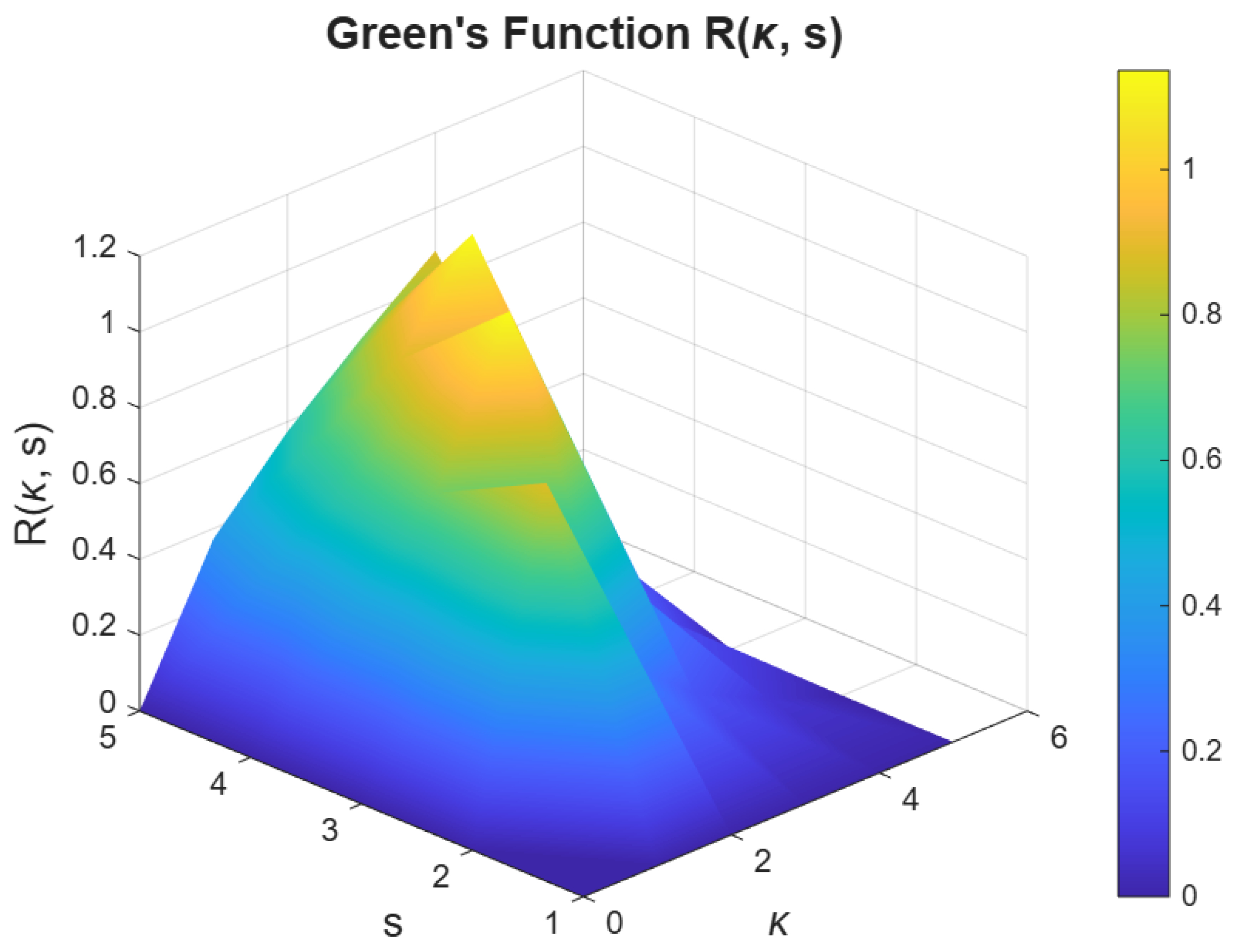
The reader can see Figure 1 and Table 1, where the values of the related Green’s functions for Examples 1 and 2 are given.

7. Conclusions

In this work, we have studied a new class of mixed-order nabla fractional boundary value problems with Dirichlet conditions. We obtain the related Green’s function and deduce several useful properties of it, which is the main mathematical novelty of this paper. These properties allow us to establish some uniqueness, existence, and multiplicity results for the considered problem. Furthermore, following the novel idea of this work, the present study can be extended in the future to cover higher-order operators or nonlinear systems coupled to different boundary conditions.

Author Contributions

Conceptualization, N.D.D. and J.M.J.; software, N.D.D. and J.M.J.; formal analysis, N.D.D. and J.M.J.; methodology, N.D.D. and J.M.J.; writing—original draft preparation, N.D.D. and J.M.J.; investigation, N.D.D. and J.M.J.; writing—review and editing, N.D.D. and J.M.J.; validation, N.D.D. and J.M.J.; visualization, N.D.D. and J.M.J.; supervision, N.D.D. and J.M.J.; resources, N.D.D. and J.M.J.; project administration, N.D.D. and J.M.J.; data curation, N.D.D. and J.M.J.; funding acquisition, N.D.D. All authors have read and agreed to the published version of the manuscript.

Funding

This study was supported by the European Union through the Program “Research, innovation and digitalization for smart transformation 2021–2027” and by the Center of Competence project “Blue Coastal Marine and Riverine Innovative & Sustainable Management of Environments and Resources (Blue Cristal)”, contract No. BG16RFPR002-1.014-0016-C01.

Data Availability Statement

The original contributions presented in this study are included in the article. Further inquiries can be directed to the corresponding author.

Acknowledgments

The authors thank the anonymous referees for their useful comments that have contributed to improving this paper.

Conflicts of Interest

The authors declare no conflicts of interest.

References

  1. Baba, I.A.; Ghanbari, B. Existence and uniqueness of solution of a fractional order tuberculosis model. Eur. Phys. J. Plus 2019, 134, 489. [Google Scholar] [CrossRef] [Scilit]
  2. Naik, P.A.; Zu, J.; Owolabi, K.M. Global dynamics of a fractional order model for the transmission of HIV epidemic with optimal control. Chaos Solitons Fractals 2020, 138, 109826. [Google Scholar] [CrossRef] [Scilit] [PubMed]
  3. Area, I.; Batarfi, H.; Losada, J.; Nieto, J.J.; Shammakh, W.; Torres, Á. On a fractional order Ebola epidemic model. Adv. Differ. Equ. 2015, 2015, 278. [Google Scholar] [CrossRef] [Scilit]
  4. Agarwal, R.; Airan, P.; Agarwal, R.P. Exploring the Landscape of Fractional-Order Models in Epidemiology: A Comparative Simulation Study. Axioms 2024, 13, 545. [Google Scholar] [CrossRef] [Scilit]
  5. Atici, F.M.; Eloe, P.W. A transform method in discrete fractional calculus. Int. J. Differ. Equ. 2007, 2, 165–176. [Google Scholar]
  6. Atici, F.M.; Eloe, P.W. Initial value problems in discrete fractional calculus. Proc. Am. Math. Soc. 2009, 137, 981–989. [Google Scholar] [CrossRef] [Scilit]
  7. Atici, F.M.; Eloe, P.W. Two-point boundary value problems for finite fractional difference equations. J. Differ. Equ. Appl. 2011, 17, 445–456. [Google Scholar] [CrossRef] [Scilit]
  8. Henderson, J. Nontrivial solutions for a nonlinear ζ-th order Atici–Eloe fractional difference equation satisfying Dirichlet boundary conditions. Differ. Equ. Appl. 2022, 14, 137–143. [Google Scholar] [CrossRef] [Scilit]
  9. Ahrendt, K.; Kissler, C. Green’s function for higher-order boundary value problems involving a nabla Caputo fractional operator. J. Differ. Equ. Appl. 2019, 25, 788–800. [Google Scholar] [CrossRef] [Scilit]
  10. Ikram, A. Lyapunov inequalities for nabla Caputo boundary value problems. J. Differ. Equ. Appl. 2019, 25, 757–775. [Google Scholar] [CrossRef] [Scilit]
  11. Liu, X.; Jia, B.; Gensler, S.; Erbe, L.; Peterson, A. Convergence of approximate solutions to nonlinear Caputo nabla fractional difference equations with boundary conditions. Electron. J. Differ. Equ. 2020, 2020, 1–19. [Google Scholar] [CrossRef] [Scilit]
  12. Peterson, A.; Hu, W. Caputo nabla fractional boundary value problems. In Progress on Difference Equations and Discrete Dynamical Systems: 25th ICDEA, London, UK, 24–28 June 2019; Springer Proceedings in Mathematics & Statistics; Springer: Cham, Switzerland, 2020; Volume 341. [Google Scholar]
  13. Gray, H.L.; Zhang, N.F. On a new definition of the fractional difference. Math. Comput. 1988, 50, 513–529. [Google Scholar] [CrossRef]
  14. Atici, F.M.; Eloe, P.W. Discrete fractional calculus with the nabla operator. Electron. J. Qual. Theory Differ. Equ. 2009, 2009, 1–12. [Google Scholar] [CrossRef] [Scilit]
  15. Anastassiou, G.A. Nabla discrete fractional calculus and nabla inequalities. Math. Comput. Model. 2010, 51, 562–571. [Google Scholar] [CrossRef] [Scilit]
  16. Heymans, N.; Podlubny, I. Physical interpretation of initial conditions for fractional differential equations with Riemann–Liouville fractional derivatives. Rheol. Acta 2006, 45, 765–771. [Google Scholar] [CrossRef] [Scilit]
  17. Kilbas, A.A.; Srivastava, H.H.; Trujillo, J.J. Theory and Applications of Fractional Differential Equations; Elsevier: Amsterdam, The Netherlands, 2006. [Google Scholar]
  18. Magin, R.L. Fractional Calculus in Bioengineering; Begell House Publisher: Danbury, CT, USA, 2006. [Google Scholar]
  19. Podlubny, I. Fractional Differential Equations; Academic Press: San Diego, CA, USA, 1999. [Google Scholar]
  20. Samko, S.G.; Kilbas, A.A.; Marichev, O.I. Fractional Integrals and Derivatives—Theory and Applications; Gordon & Breach: Linghorne, PA, USA, 1993. [Google Scholar]
  21. West, B.J.; Bologna, M.; Grigolini, P. Physics of Fractal Operators; Springer: New York, NY, USA, 2003. [Google Scholar]
  22. Miller, K.S.; Ross, B. Fractional Difference Calculus. Univalent Functions, Fractional Calculus, and Their Applications; Ellis Horwood Series in Mathematics and Its Applications; Horwood: Chichester, UK, 1989. [Google Scholar]
  23. Bohner, M.; Peterson, A. Dynamic Equations on Time Scales: An Introduction with Applications; Springer: Boston, MA, USA, 2001. [Google Scholar]
  24. Goodrich, C.; Peterson, A.C. Discrete Fractional Calculus; Springer: Cham, Switzerland, 2015. [Google Scholar]
  25. Ferreira, R.A.C. Discrete Fractional Calculus and Fractional Difference Equations; Springer Briefs in Mathematics; Springer: Cham, Switzerland, 2022. [Google Scholar]
  26. Ahrendt, K.; Castle, L.; Holm, M.; Yochman, K. Laplace transforms for the nabla-difference operator and a fractional variation of parameters formula. Commun. Appl. Anal. 2012, 16, 317–348. [Google Scholar]
  27. Bastos, N.; Torres, D. Combined delta-nabla sum operator in discrete fractional calculus. Commun. Frac. Calc. 2010, 2010, 41–47. [Google Scholar]
  28. Gholami, Y.; Ghanbari, K. Coupled systems of fractional ∇-difference boundary value problems. Differ. Equ. Appl. 2016, 8, 459–470. [Google Scholar] [CrossRef] [Scilit]
  29. Dimitrov, N.D.; Jonnalagadda, J.M. Existence Results for Nabla Fractional Problems with Anti-Periodic Boundary Conditions. Mathematics 2025, 13, 2487. [Google Scholar] [CrossRef] [Scilit]
  30. Graef, J.; Kong, L.; Kong, Q.; Wang, M. A fractional boundary value problem with Dirichlet boundary conditions. Commun. Appl. Anal. 2015, 19, 497–504. [Google Scholar]
  31. Graef, J.; Wang, M.; Yost, G. Nonlinear Fractional Boundary Value Problem Involving Riemann–Liouville Fractional Derivatives of Two Different Orders. Commun. Appl. Nonlinear Anal. 2016, 23, 93–102. [Google Scholar]
  32. Eloe, P.W.; Neugebauer, J.T. Green’s Functions for a Fractional Boundary Value Problem with Three Terms. Foundations 2022, 2, 885–897. [Google Scholar] [CrossRef] [Scilit]
  33. Panigrahi, S.; Kumar, R. Existence and non-existence of positive solutions for a class of fractional boundary value problems. Filomat 2025, 39, 3099–3125. [Google Scholar] [CrossRef] [Scilit]
  34. Dimitrov, N.D.; Jonnalagadda, J.M. Existence of Positive Solutions for a Class of Nabla Fractional Boundary Value Problems. Fractal Fract. 2025, 9, 131. [Google Scholar] [CrossRef] [Scilit]
  35. Dimitrov, N.D.; Jonnalagadda, J.M. Multiple Positive Solutions of Nabla Fractional Equations with Summation Boundaries. Mathematics 2025, 13, 3210. [Google Scholar] [CrossRef] [Scilit]
  36. Dimitrov, N.D.; Jonnalagadda, J.M. Positive Solutions for Nabla Fractional Three-Point Boundary Value Problems. Mathematics 2026, 14, 1086. [Google Scholar] [CrossRef] [Scilit]
  37. Cabada, A.; Dimitrov, N.; Jagan Mohan, J. Green’s functions for fractional difference equations with Dirichlet boundary conditions. Chaos Solitons Fractals 2021, 153, 111455. [Google Scholar] [CrossRef] [Scilit]
  38. Cabada, A.; Dimitrov, N.; Jagan Mohan, J. Green’s functions and existence of solutions of nonlinear fractional implicit difference equations with Dirichlet boundary conditions. Opusc. Math. 2024, 44, 167–195. [Google Scholar] [CrossRef] [Scilit]
  39. Chen, Y.; Xu, J.; Tai, Y.; Xu, X.; Chen, N. Critical damping design method of vibration isolation system with both fractional-order inerter and damper. Mech. Adv. Mater. Struct. 2022, 29, 1348–1359. [Google Scholar] [CrossRef] [Scilit]
  40. Li, Y.; Duan, J.-S. The periodic response of a fractional oscillator with a spring-pot and an inerter-pot. J. Mech. 2021, 37, 108–117. [Google Scholar] [CrossRef] [Scilit]
  41. Agarwal, R.; Meehan, M.; O’Regan, D. Fixed Point Theory and Applications; Cambridge University Press: Cambridge, UK, 2001. [Google Scholar]
  42. Cabada, A.; Dimitrov, N. Existence of Solutions of nth-Order Nonlinear Difference Equations with General Boundary Conditions. Acta Math. Sci. 2020, 40, 226–236. [Google Scholar] [CrossRef] [Scilit]
Figure 1. Values of R κ , s in Examples 1 and 2.
Fractalfract 10 00641 g001
Table 1. Values of the Green’s function considered in Examples 1 and 2.
s = 1 s = 2 s = 3 s = 4 s = 5
κ = 0 00000
κ = 1 0 0.88778 0.73843 0.57442 0.37333
κ = 2 0 0.33506 1.13620 0.88384 0.57442
κ = 3 0 0.16975 0.42968 1.13620 0.73843
κ = 4 0 0.071982 0.16975 0.33506 0.88778
κ = 5 00000
Disclaimer/Publisher’s Note: The statements, opinions and data contained in all publications are solely those of the individual author(s) and contributor(s) and not of MDPI and/or the editor(s). MDPI and/or the editor(s) disclaim responsibility for any injury to people or property resulting from any ideas, methods, instructions or products referred to in the content.