Event-Triggered Quantized Synchronization via Sampled-Data Iterative Learning Control for Coupled Fractional-Order Time-Delayed Competitive Neural Networks

Abstract

This paper examines the problem of achieving synchronization within fractional-order competitive neural networks (FOCNNs) affected by intrinsic transmission delays. To overcome the limitations associated with restricted network bandwidth and excessive computational expenses, a quantized sampled-data distributed iterative learning control (QSDILC) strategy is introduced. In contrast to conventional continuous-time methods, a precise quantizer and a variable sampling structure are explicitly integrated into the presented QSDILC law. Within this framework, the control trajectory of each individual node is adjusted relying entirely upon discretized, locally acquired error signals. Furthermore, an event-triggering scheme founded on the error energy attenuation (EEA) principle is formulated to maximize communication efficiency. Control signal refreshes are adaptively managed by this EEA-driven approach through the continuous tracking of how rapidly the synchronization error energy decays. Consequently, unnecessary iterative steps are eliminated while the strict convergence of the FOCNN states along the iteration axis is guaranteed. Through theoretical evaluation—relying on the fundamentals of fractional calculus and contraction mapping theory—the necessary criteria guaranteeing synchronization under the proposed QSDILC architecture are rigorously established. Numerical simulations demonstrate that communication overhead and computational burdens are significantly minimized by the integrated QSDILC and EEA-based event-triggered approach, all while a superior convergence speed is maintained, thereby offering a reference for addressing the synchronization control of time-delayed FOCNNs under limited communication and computational resources.

1. Introduction

In the past few decades, the collective dynamics of complex dynamical networks have attracted substantial multidisciplinary interest due to their extensive applications in diverse fields such as image processing, secure communication, and social network analysis [1,2]. Among various network collective behaviors, consensus synchronization—where all nodes in a coupled network reach a consistent state through localized interactions—has emerged as a fundamental research topic [3,4,5]. Particularly, competitive neural networks, which incorporate both excitatory and inhibitory interactions between neurons, have demonstrated remarkable capabilities in modeling biological systems, pattern recognition [6,7], and associative memory. When dealing with practical neural activities, biological processes often exhibit intrinsic memory and hereditary properties. Fractional-order calculus, characterized by its non-locality and long-term memory, provides a more accurate mathematical tool than traditional integer-order models to characterize these phenomena [8,9]. Consequently, investigating the synchronization of fractional-order competitive neural networks (FOCNNs) is of paramount theoretical and practical significance [10,11,12]. Under numerous engineering frameworks, the completion of synchronization objectives within a bounded duration is demanded of neural systems [13]. To handle operations that exhibit a periodic or repeating pattern, iterative learning control (ILC) has emerged as a highly powerful methodology [14,15].

Iterative learning control (ILC) is characterized by the strategic utilization of historical tracking data obtained from prior operations to update the control input, whereby highly precise tracking performance is successfully realized for plants executing recurrent missions within a prescribed duration. The evolution of distributed ILC has further enabled the coordination of multi-agent neural ensembles [16], where nodes update their behaviors based on neighboring information. Moreover, the implementation of distributed ILC in FOCNNs is often hampered by signal transmission latencies and the high dimensionality of neural states. Time-delays, in particular, can severely degrade synchronization performance, lead to sluggish response, or even induce oscillation and instability along the iteration axis. References [17,18] study the use of iterative learning control algorithms to handle multi-agent systems with time delays, achieving both stable and effective synchronization in such settings.

In modern networked environments, excessive demands are placed on communication bandwidth and computational resources due to the uninterrupted transmission of high-precision state variables among coupled nodes. To alleviate this transmission bottleneck, widespread applications have been found for sampled-data control and event-triggered strategies [19,20,21]. Sampled-data ILC updates the control signal only at discrete time instants, which aligns with the digital nature of modern communication channels. However, fixed-period sampling may still result in redundant data transmission when the synchronization error is already sufficiently small. Non-periodic event-triggered control can further address this issue. Although conventional event-triggered schemes can reduce unnecessary updates by monitoring error thresholds, they often lack a rigorous connection to the fundamental energy dissipation properties of the system. A solution is presented by an event-triggered scheme constructed upon the error energy attenuation (EEA) framework, in which control actions are updated in accordance with the decay speed of the synchronization error energy. Furthermore, for bandwidth-constrained digital transmission links, the implementation of signal quantization—under which a discrete array of values is mapped from continuous-time variables—is practically unavoidable. Convergence analysis of distributed ILC with quantified uncertainty, non-periodic EEA-based event-triggered updates, and fractional-order genetic effects is a topic worthy of further study. References [22,23] applied iterative learning control combined with the EEA-based event-triggered mechanisms to multi-agent systems and traditional nonlinear systems, respectively, achieving good convergence in both synchronization and tracking.

Driven by the above-mentioned incentives, the output synchronization consensus problem for FOCNNs featuring time delays is investigated in this study within a quantized sampled-data distributed iterative learning control (QSDILC) framework. As far as the authors are aware, a pioneering attempt is represented here to incorporate the EEA-driven triggering law within the fractional-order iterative learning scheme for neural networks experiencing both transmission delays and bandwidth limitations. Specifically, synthesis of a P-type sampled-data distributed learning protocol is driven by the EEA-based event-triggering strategy, where the control trajectory is updated exclusively when the synchronization error energy fails to attenuate according to a prescribed dissipative law. By employing the sector-bound property of logarithmic quantizers and fractional-order integral inequalities, sufficient conditions for iterative convergence are rigorously derived.

The main features and core contributions of this study are outlined below

(i)

For FOCNNs, a distributed P-type learning scheme is formulated by incorporating logarithmic quantization alongside a non-continuous sampling mechanism into a novel control framework, which is characterized as a QSDILC protocol, so as to satisfy the transmission specifications of digital communication networks.

(ii)

By integrating the standard error-threshold-based event triggered by the proposed error-energy-attenuation mechanism, the protocol achieves a superior trade-off between output synchronization precision and communication efficiency. The EEA-based event-triggered mechanism prunes redundant iterations from an energy-dissipation perspective, ensuring rapid convergence while minimizing the usage of communication bandwidth.

(iii)

A unified analytical platform is established to guarantee global consensus output synchronization despite the presence of transmission time-delays, quantization uncertainties, and non-smooth triggers. By utilizing fractional-order Bellman–Gronwall analysis and contraction mapping principle, the robust convergence along the iteration axis is rigorously proved.

The remainder of this paper is organized as follows. Section 2 provides the necessary mathematical preliminaries. Section 3 presents the description of the FOCNN model and the formal definition of control objectives. Section 4 introduces the proposed event-excited EEA-based triggering mechanism, the design of the QSDILC protocol, and elaborates on the scaling techniques for fractional-order integral terms involving time-delays. In Section 5, the convergence conditions are derived, and the theoretical stability is rigorously proved. Numerical simulations are provided in Section 6 to verify the theoretical results and demonstrate the effectiveness of the QSDILC algorithm. Section 7 provides a comprehensive conclusion of the entire paper.

• Notations: Throughout this paper, the n-dimensional Euclidean space is represented by ${\mathbb{R}}^n$. Let $Q^T$ denote the transpose of a given matrix Q, and let the operator ⊗ signify the Kronecker product. An identity matrix with dimensions $q\times q$ is symbolized by $I_q$. Regarding a matrix $Q\in {\mathbb{R}}^q$, its norm is evaluated via $\parallel Q\parallel =\sqrt{{\lambda }_{max}\left(Q^{T}Q\right)}$, in which the largest eigenvalue of the argument is yielded by ${\lambda }_{max}(·)$. For a vector-valued function $h\left(t\right):[0,T]\to {\mathbb{R}}^n$, its $\lambda$-norm is formulated as ${\parallel h\parallel }_{\lambda }={sup}_{t\in [0,T]}\{e^{-\lambda t}\parallel h\left(t\right)\parallel \}$, with $\lambda$ being a positive real constant. Additionally, the floor and sign operations are respectively denoted by $\lfloor ·\rfloor$ and $\mathrm{sign}(·)$.

2. Preliminaries

To establish a rigorous theoretical framework for the proposed FOCNNs network architecture, this section is organized into three aspects. First, the graph-theoretic foundations governing the structural topology of the model are delineated. Building upon this spatial context, essential definitions of fractional calculus are introduced. Finally, the logarithmic quantization schemes employed within the FOCNNs are detailed.

2.1. Graph Theory

A directed graph $\mathcal{G}=[\mathcal{V},\mathcal{E},\mathcal{A}]$ is commonly employed to describe the communication topology of a complex neural network with interacting agents. It consists of a node set $\mathcal{V}=\{1,2,\cdots ,N\}$ and an edge set $\mathcal{E}\subseteq \mathcal{V}\times \mathcal{V}$, where $(i,j)\in \mathcal{E}$ denotes a directed edge from node i to node j. The adjacency matrix $\mathcal{A}={\left[a_{ij}\right]}_{N\times N}$ of $\mathcal{G}$ is defined such that $a_{ij}=1$ if $(j,i)\in \mathcal{E}$ and $a_{ij}=0$ otherwise, with $a_{ii}=0$ for all i.

The Laplacian matrix $\mathcal{L}={\left[l_{ij}\right]}_{N\times N}$ of the digraph is given by

$$l_{ij}=\left\{\begin{array}{c}-a_{ij},i\ne j,\hfill \\ {\displaystyle {\sum }_{k=1,k\ne i}^N}{a}_{ik}=d_i,i=j,\hfill \end{array}\right.$$

where $d_i$ represents the in-degree of the i-th node. Correspondingly, the degree matrix is $\Omega =\mathrm{diag}\{d_1,\dots ,d_N\}$, and it follows that $\mathcal{L}=\Omega -\mathcal{A}$. A directed graph is said to contain a spanning tree if there exists a root node from which every other node can be reached via a directed path.

2.2. Fractional-Order Calculus

Fractional-order calculus is a generalization of classical calculus that extends the operations of differentiation and integration to non-integer orders.

Definition 1

([24]). For a function $g\left(t\right):{\mathbb{R}}^{+}\mapsto \mathbb{R}$, the Riemann–Liouville fractional-order integral with order $\alpha >0$ is defined as

$${}_{t_0}\mathcal{D}_t^{-\alpha }g\left(t\right)\triangleq {\displaystyle \frac{1}{\Xi \left(\alpha \right)}}{\int }_{t_0}^t{(t-s)}^{\alpha -1}g\left(s\right)ds,$$

where $\Xi (·)$ stands for the Gamma function.

Definition 2

([17]). Let $\alpha >0$ be a given real number. The formulation of the Caputo fractional-order derivative is given by

$${}_{t_0}{}^C\mathcal{D}_t^{\alpha }g\left(t\right)\triangleq {}_{t_0}\mathcal{D}_t^{\alpha -\iota }\left({\mathcal{D}}^{\iota }g\left(t\right)\right),\iota -1\le \alpha <\iota ,\iota \in \mathbb{N}.$$

For simplicity, the Caputo derivative ${}_{t_0}{}^C\mathcal{D}_t^{\alpha }$ is denoted by ${\mathcal{D}}_t^{\alpha }$ in the subsequent section.

Definition 3

([25]). The two-parameter function of the Mittag–Leffler function is defined by

$$E_{\alpha ,\beta }\left(z\right)={\displaystyle \sum _{k=0}^{\infty }}{\displaystyle \frac{z^k}{\Xi (\alpha k+\beta )}},\alpha >0,\beta >0,z\in \mathbb{C}.$$

To establish a rigorous theoretical foundation for the subsequent stability analysis and convergence proofs, several essential lemmas are introduced.

Lemma 1

([26]). The fractional-order derivative or integral of the Mittag–Leffler function satisfies

$${}_{t_0}\mathcal{D}_t^{\vartheta }\left[{(t-t_0)}^{\beta -1}{E}_{\alpha ,\beta }\left(\lambda {(t-t_0)}^{\alpha }\right)\right]={(t-t_0)}^{\beta -\vartheta -1}{E}_{\alpha ,\beta -\vartheta }\left(\lambda {(t-t_0)}^{\alpha }\right),\vartheta <\beta .$$

Lemma 2

([27]). Let $u\left(t\right)$ be a continuous function on $t\in [0,T]$, and let $v(t-\tau )$ be continuous and nonnegative on the domain $0\le \tau \le T$. Moreover, let $w\left(t\right)$ be a positive continuous and non-decreasing function on $t\in [0,T]$.

If

$$u\left(t\right)\le w\left(t\right)+{\int }_0^{t}v(t-\tau )u\left(\tau \right)d\tau ,t\in [0,T],$$

then

$$u\left(t\right)\le w\left(t\right)e^{{\int }_0^{t}v(t-\tau )d\tau },t\in [0,T].$$

Lemma 3

([28]). If the function $f(t,x(t\left)\right)$ is continuous, then the initial value problem

$$\left\{\begin{array}{c}{}_{t_0}{}^C\mathcal{D}_t^{\alpha }x\left(t\right)=f(t,x\left(t\right)),0<\alpha <1\hfill \\ x\left(t_0\right)=x\left(0\right),\hfill \end{array}\right.$$

is equivalent to the nonlinear Volterra integral equation

$$x\left(t\right)=x\left(0\right)+{\displaystyle \frac{1}{\Xi \left(\alpha \right)}}{\int }_0^t{(t-s)}^{\alpha -1}f(s,x\left(s\right))ds,$$

and its solutions are continuous.

2.3. Conception of Logarithmic Quantization

To mitigate the communication burden and data redundancy in the transmission channel, a logarithmic quantizer $\mathcal{Q}(·):\mathbb{R}\to \Theta$ is strategically integrated into the control framework. The set of quantized levels $\Theta$ is formulated as a discrete yet infinite manifold

$$\begin{array}{c}\hfill \Theta =\left\{\pm {\omega }_i:{\omega }_i={\rho }_1^i{\omega }_0,i=0,\pm 1,\pm 2,\dots \right\}\cup \left\{0\right\},0<{\rho }_1<1,{\omega }_0>0\end{array}$$

where $\rho$ denotes the quantization density. The mapping $\mathcal{Q}\left(e\right)$ projects the continuous error signal onto the nearest quantization level ${\omega }_i\mathrm{sign}\left(e\right)$ within a specific sector. From a robust control perspective, the induced quantization error is characterized by the sector bound condition [29]: $\mathcal{Q}\left(e\right)-e=\Delta e$, where the uncertainty term $\Delta$ is strictly confined within the compact interval $[-\varpi ,\varpi ]$ with $\varpi ={\displaystyle \frac{1-{\rho }_1}{1+{\rho }_1}}$. This formulation elegantly transforms the non-smooth quantization effect into a bounded multiplicative perturbation, facilitating the subsequent convergence analysis via the contraction mapping principle.

3. System Description and Problem Statement

Building upon the mathematical preliminaries established above, an in-depth analytical investigation into the FOCNNs is conducted in this subsection. To rigorously evaluate the dynamic behavior of the proposed architecture, the primary stability objectives and convergence criteria are explicitly formulated. Furthermore, to facilitate a tractable and robust systemic analysis, a set of fundamental assumptions is established.

The Description of Delayed FOCNNs

The dynamical architecture of the considered n-dimensional delayed FOCNNs is formulated by a set of coupled Caputo fractional differential equations as follows

$$\begin{array}{c}\hfill \left\{\begin{array}{ccc}\hfill {\mathcal{D}}_t^{\alpha }{x}_i\left(t\right)& =& -d_i{x}_i\left(t\right)+{\displaystyle \sum _{j=1}^n}{a}_{ij}{f}_j\left(x_j\left(t\right)\right)+{\iota }_i{o}_i\left(t\right)+{\displaystyle \sum _{j=1}^n}{b}_{ij}{f}_j\left(x_i(t-\tau )\right)+J_i\hfill \\ \hfill {\mathcal{D}}_t^{\alpha }{o}_i\left(t\right)& =& -c_i{o}_i\left(t\right)+{\vartheta }_i{f}_i\left(x_i\left(t\right)\right),\hfill \end{array}\right.\end{array}$$

(1)

where $i=1,2,\dots ,n$ serves as the node index within the neural ensemble. In this framework, ${\mathcal{D}}_t^{\alpha }$ denotes the Caputo fractional derivative operator of order $\alpha \in (0,1)$, characterizing the hereditary and memory effects inherent in neural activity. The state variables $x_i\left(t\right)$ and $o_i\left(t\right)$ represent the neuron potential and synaptic efficiency, respectively. The structural parameters $a_{ij}$ and $b_{ij}$ define the interconnection weights, while $J_i$ signifies the external stimuli. $f_i(·)$ and $f_j(·)$ denote the activation functions of the i-th and j-th neurons. The positive coefficients $d_i$, $c_i$, and $b_i$ describe the self-inhibitory and gain attributes of the nodes. To account for signal transmission latencies, a time delay $\tau >0$ is incorporated into the activation function $f_j(·)$. The initial state of the FOCNNs is stipulated by the continuous vector function $x_{i,k}\left(s\right)={\phi }_{i,k}\left(s\right)$ for $s\in [-\tau ,0]$.

To facilitate a more compact analytical framework, the scalar dynamics are first encapsulated into a vectorized form by introducing $x\left(t\right)={[x_1\left(t\right),x_2\left(t\right),\dots ,x_n\left(t\right)]}^T$, $o\left(t\right)={[o_1\left(t\right),o_2\left(t\right),\dots ,o_n\left(t\right)]}^T$, and the external stimuli vector $J={[J_1,J_2,\dots ,J_n]}^T$. To simplify the notation without loss of generality, the same activation function, denoted by $f(·)$, is assumed to be shared by all neurons. The FOCNNs’ parameters are defined by the diagonal matrices $D=\mathrm{diag}\{d_1,d_2,\dots ,d_n\}$, $A=\mathrm{diag}\{{\iota }_1,{\iota }_2,\dots ,{\iota }_n\}$, $B=\mathrm{diag}\{{\vartheta }_1,{\vartheta }_2,\dots ,{\vartheta }_n\}$, and $C=\mathrm{diag}\{c_1,c_2,\dots ,c_n\}$, along with the interconnection weight matrices $\widehat{A}={\left(a_{ij}\right)}_{n\times n}$ and $\widehat{B}={\left(b_{ij}\right)}_{n\times n}$. The FOCNNs (1) is reformulated as

$$\begin{array}{c}\hfill \left\{\begin{array}{ccc}\hfill {\mathcal{D}}_t^{\alpha }x\left(t\right)& =& -Dx\left(t\right)+\widehat{A}f\left(x\left(t\right)\right)+Ao\left(t\right)+\widehat{B}f\left(x(t-\tau )\right)+J\hfill \\ \hfill {\mathcal{D}}_t^{\alpha }o\left(t\right)& =& -Co\left(t\right)+Bf\left(x\right(t\left)\right).\hfill \end{array}\right.\end{array}$$

By utilizing the matrix lifting technique, the augmented state vector $z\left(t\right)={\left[\begin{array}{c}{x}^T\left(t\right),o^T\left(t\right)\end{array}\right]}^T$ allows the above FOCNNs to be transformed into the following unified representation

$$\begin{array}{c}\hfill {\mathcal{D}}_t^{\alpha }z\left(t\right)=\tilde{A}z\left(t\right)+\tilde{B}f\left(z\left(t\right)\right)+\tilde{C}f\left(z(t-\tau )\right)+\tilde{J},\end{array}$$

with $\tilde{A}=\left[\begin{array}{cc}-D& A\\ 0& -C\end{array}\right]$, $\tilde{B}=\left[\begin{array}{cc}\widehat{A}& 0\\ 0& B\end{array}\right]$, $\tilde{C}=\left[\begin{array}{cc}\widehat{B}& 0\\ 0& 0\end{array}\right]$, and $\tilde{J}=\left[\begin{array}{c}J\\ 0\end{array}\right]$.

Consider a coupled network consisting of N such FOCNNs, where the communication topology is characterized by a directed digraph $\mathcal{G}=\{\mathcal{V},\mathcal{E},\mathcal{A}\}$ and its associated Laplacian matrix $\mathcal{L}$. The dynamics of the i-th node within the coupled ensemble are governed by

$$\begin{array}{c}\hfill {\mathcal{D}}_t^{\alpha }{z}_i\left(t\right)=\tilde{A}{z}_i\left(t\right)+\tilde{B}f\left(z_i\left(t\right)\right)+\tilde{C}f\left(z_i(t-\tau )\right)+\tilde{D}{u}_i\left(t\right)-c{\displaystyle \sum _{j=0}^N}{\mathcal{L}}_{ij}\Psi z_j\left(t\right)+\tilde{J},\end{array}$$

where $u_i\left(t\right)\in {\mathbb{R}}^{2n}$ denotes the control input, $c>0$ represents the coupling strength, and $\Psi \in {\mathbb{R}}^{2n\times 2n}$ is a positive-definite inner coupling matrix.

By incorporating the output equation $y_i\left(t\right)=E{z}_i\left(t\right)+F{u}_i\left(t\right)$, where E is the output state matrix, and F is the direct feedthrough matrix, the FOCNNs is summarized as

$$\begin{array}{c}\hfill \left\{\begin{array}{cc}& {\mathcal{D}}_t^{\alpha }{z}_i\left(t\right)=\tilde{A}{z}_i\left(t\right)+\tilde{B}f\left(z_i\left(t\right)\right)+\tilde{C}f\left(z_i(t-\tau )\right)+\tilde{D}{u}_i\left(t\right)-c{\displaystyle {\sum }_{j=0}^N}{\mathcal{L}}_{ij}\Psi z_j\left(t\right)+\tilde{J}\\ & y_i\left(t\right)=E{z}_i\left(t\right)+F{u}_i\left(t\right).\end{array}\right.\end{array}$$

To characterize a predetermined output synchronization target $y_d\left(t\right)$, the reference framework over a finite time interval $t\in [0,T]$ is modeled by

$$\begin{array}{c}\hfill \left\{\begin{array}{cc}& {\mathcal{D}}_t^{\alpha }{z}_d\left(t\right)=\tilde{A}{z}_d\left(t\right)+\tilde{B}f\left(z_d\left(t\right)\right)+\tilde{C}f\left(z_d(t-\tau )\right)+\tilde{D}{u}_d\left(t\right)-c{\displaystyle {\sum }_{j=0}^N}{\mathcal{L}}_{ij}\Psi z_d\left(t\right)+\tilde{J},\\ & y_d\left(t\right)=E{z}_d\left(t\right)+F{u}_d\left(t\right).\end{array}\right.\end{array}$$

(2)

The desired initial conditions for the FOCNNs with time-delay are explicitly defined by the continuous function $z_d\left(s\right)={\phi }_d\left(s\right)$ for all $s\in [-\tau ,0]$.

An augmented directed graph denoted by $\overline{\mathcal{G}}=\{\mathcal{V}\cup \left\{0\right\},\overline{\mathcal{E}},\overline{\mathcal{A}}\}$ is employed to characterize the expanded topological interaction, where the existence of a spanning tree is guaranteed within $\overline{\mathcal{G}}$.

The ultimate output synchronization objective is to synthesize an appropriate sequence of control inputs $u_{i,k}\left(t\right)$ such that the output synchronization error vanishes as the iteration number k tends to infinity.

To establish a rigorous theoretical foundation for the proposed control architecture, this section delineates the fundamental assumptions regarding the FOCNNs’ dynamics, topological structure, and iterative initializations. These prerequisites are essential to ensure the existence, uniqueness, and subsequent convergence of the output synchronization manifold for the coupled FOCNNs.

Assumption 1.

$f(·)$ represents the activation function and meets the Lipschitz condition, that is, there exists a positive constant $l_f$ for all $z_i\in {\mathbb{R}}^{2n}$ such that

$$∥f\left(z_1\right)-f\left(z_2\right)∥⩽l_f∥z_1-z_2∥,z_i\in {\mathbb{R}}^{2n}.$$

Assumption 2.

For the delayed FOCNNs, the initial states on the interval $[-\tau ,0]$ are specified by

$$z_{i,k}\left(\kappa \right)=z_d\left(\kappa \right),\kappa \in [-\tau ,0],i\in \mathcal{V}.$$

4. Synchronization for Time-Delayed FOCNNs

In this part, the synthesis of the QSDILC law is detailed, and the triggering criteria associated with the EEA-driven mechanism within the FOCNNs are subsequently established. Furthermore, fractional integrals containing time delay terms will be appropriately scaled.

4.1. Design of the Sampling Mechanism in the QSDILC Protocol

Regarding the continuous-time framework, the total interval $[0,T]$ is segmented into M sub-intervals of width h via a dedicated sampling device. $\mathcal{H}=\{0,1,2,\dots ,M\}$ denotes the discrete index of the sampled indices, and $M=\lfloor {\displaystyle \frac{T}{h}}\rfloor$. The expression for the distributed synchronization error in the output space is formulated as follows

$${\xi }_{i,k}\left(t\right)={\upsilon }_i(y_d\left(t\right)-y_{i,k}\left(t\right))+\sum _{j\in \mathcal{V}}{a}_{ij}(y_{j,k}\left(t\right)-y_{i,k}\left(t\right)),$$

wherein $v_i$ signifies the coupling strength connecting the i-th FOCNN to the virtual reference agent. In particular, $v_i>0$ is assigned whenever the node receives direct information from the reference agent, whereas $v_i=0$ is assigned otherwise ${\upsilon }_i=0$, with $\mathcal{B}=\mathrm{diag}\{{\upsilon }_1,{\upsilon }_2,\dots ,{\upsilon }_N\}$ characterizing the pinning gain manifold.

Based on the sampled-data QSDILC protocol, we establish the synchronization result at sampling points. The primary control goal is to guarantee that the output synchronization error asymptotically converges to zero as the iteration index k approaches infinity for all sampling instances $rh$; that is

$$\underset{k\to \infty }{lim}\sum _{i,j\in \mathcal{V}}∥y_{i,k}\left(rh\right)-y_{j,k}\left(rh\right)∥=0,\forall r\in \mathcal{H}.$$

During the $(k+1)$-th iteration trial, the mathematical framework of the quantized sampled-data control protocol designed for the i-th agent is specified as follows

$$\left\{\begin{array}{c}{u}_{i,k+1}\left(t\right)=u_{i,k}\left(t\right)+\Gamma \mathcal{Q}\left({\xi }_{i,k}\left(t\right)\right),t\in [rh,rh+h)\hfill \\ u_{i,k+1}\left(t\right)=u_{i,k+1}\left(rh\right),\hfill \end{array}\right.$$

in which the learning gain matrix is designated as $\Gamma \in {\mathbb{R}}^{2n\times 2n}$.

4.2. Synthesis of the EEA-Driven Event-Triggered Framework

For the purpose of establishing the mathematical analysis, the output error $e_{i,k}\left(rh\right)$ at the k-th execution trial is utilized to characterize the deviation arising between the tracking target $y_d\left(rh\right)$ and the actual system output $y_{i,k}\left(rh\right)$ within the present control interval, yielding

$$\begin{array}{c}\hfill e_k\left(rh\right)={\left[{\left(e_{1,k}\left(rh\right)\right)}^T,\dots ,{\left(e_{N,k}\left(rh\right)\right)}^T\right]}^T,y_k\left(rh\right)={\left[{\left(y_{1,k}\left(rh\right)\right)}^T,\dots ,{\left(y_{N,k}\left(rh\right)\right)}^T\right]}^T.\end{array}$$

To regulate the discrete updating operations within the learning framework, the definition $R_k(rh+h)=e_{k_l}(rh+h)-e_k(rh+h)$ introduces the error energy manifold along the iteration axis for $k\in [k_l,k_{l+1})$. The generation of the triggering trial sequence $\left\{k_l\right\}$ is dynamically governed by an attenuation function $\chi \left(R_k(rh+h)\right)$, by which the sufficiency of error energy attenuation over successive learning runs is verified. The triggering condition is then given by

$$\{k+1=k_{l+1}\mid \chi \left(R_k(rh+h)\right)\ge 0\}.$$

The subsequent lemma provides the specific mathematical description of the EEA-based event-triggering mechanism for the considered FOCNNs.

Lemma 4.

Consider the proposed QSDILC framework. The EEA-driven execution condition $\chi \left(R_k\left((r+1)h\right)\right)$ formulated for the FOCNNs satisfies the following structure

$$\chi \left(R_k(rh+h)\right)={\parallel R_k(rh+h)\parallel }^2-{\displaystyle \frac{\eta \parallel e_k{(rh+h)\parallel }^2-2S_k(rh+h)}{2(1+\varpi ){∥\frac{h^{\alpha }}{\alpha }\frac{[(\mathcal{L}+\mathcal{B})\otimes E\tilde{D}\Gamma ]}{\Xi \left(\alpha \right)}+[(\mathcal{L}+\mathcal{B})\otimes F\Gamma ]∥}^2}},$$

the convergence rate and system robustness are well balanced by adjusting the positive scalar $\eta \in (0,1]$, which acts as a design parameter, whereas error compensation is executed by the auxiliary operator $S_k(rh+h)$ designed as

$$\begin{array}{cc}\hfill S_k(rh+h)=& ∥\left[I-\left({\displaystyle \frac{h^{\alpha }}{\alpha }}{\displaystyle \frac{[(\mathcal{L}+\mathcal{B})\otimes E\tilde{D}\Gamma ]}{\Xi \left(\alpha \right)}}+[(\mathcal{L}+\mathcal{B})\otimes F\Gamma ]\right)(1+\varpi )\right]e_k(rh+h)\hfill \\ \hfill & -(I_N\otimes E)\delta z_k\left(rh\right)-{\displaystyle \frac{(I_N\otimes E\tilde{A})}{\Xi \left(\alpha \right)}}{\int }_{rh}^{rh+h}{(rh+h-s)}^{\alpha -1}\delta z_k\left(s\right)ds\hfill \\ \hfill & -{\displaystyle \frac{(I_N\otimes E\tilde{B})}{\Xi \left(\alpha \right)}}{\int }_{rh}^{rh+h}{(rh+h-s)}^{\alpha -1}\delta f\left(z_k\left(s\right)\right)ds\hfill \\ \hfill & -{\displaystyle \frac{(I_N\otimes E\tilde{C})}{\Xi \left(\alpha \right)}}{\int }_{rh}^{rh+h}{(rh+h-s)}^{\alpha -1}\delta f\left(z_k(s-\tau )\right)ds\hfill \\ \hfill & {+{\displaystyle \frac{c(\mathcal{L}\otimes E\Psi )}{\Xi \left(\alpha \right)}}{\int }_{rh}^{rh+h}{(rh+h-s)}^{\alpha -1}\delta z_k\left(s\right)ds∥}^2.\hfill \end{array}$$

with $\delta z_k\left(t\right)=z_{k+1}\left(t\right)-z_k\left(t\right)$.

Proof. 

Utilizing the algebraic features of the Kronecker product, the compact formulation of the considered FOCNNs (2) can be mathematically cast into the collective framework

$$\left\{\begin{array}{cc}\hfill & {\mathcal{D}}_t^{\alpha }{z}_k\left(t\right)=(I_N\otimes \tilde{A})z_k\left(t\right)+(I_N\otimes \tilde{B})f\left(z_k\left(t\right)\right)+(I_N\otimes \tilde{C})f\left(z_k(t-\tau )\right)+(I_N\otimes \tilde{D})u_k\left(t\right)\hfill \\ & -c{\displaystyle {\sum }_{j=0}^N}{\mathcal{L}}_{ij}\Psi z_j\left(t\right)+(I_N\otimes \tilde{J}),\hfill \\ \hfill & y_k\left(t\right)=(I_N\otimes E)z_k\left(t\right)+(I_N\otimes F)u_k\left(t\right).\hfill \end{array}\right.$$

In light of the predefined tracking error $e_k\left(t\right)$, the recursive relation characterizing the error evolutionary trajectory can be derived as

$$\begin{array}{cc}\hfill e_{k+1}\left(t\right)& =e_k\left(t\right)+y_k\left(t\right)-y_{k+1}\left(t\right)\hfill \\ \hfill & =e_k\left(t\right)-(I_N\otimes F)\delta u_{k_l}\left(t\right)-(I_N\otimes E)\delta z_k\left(t\right),\hfill \end{array}$$

(3)

with $\delta u_{k_l}\left(t\right)=u_{k_{l+1}}\left(t\right)-u_{k_l}\left(t\right)$.

According to the established QSDILC protocol, $(I_{Nm}+\Delta (k,t))$ captures the aggregate quantization uncertainty with $\Delta (k,t)=\mathrm{diag}\{{\Delta }_1(k,t),\dots ,{\Delta }_N(k,t)\}$, the control increment $\delta u_{k_l}\left(t\right)$ is modulated by the topological interaction and quantization uncertainty as

$$\begin{array}{c}\hfill \delta u_{k_l}\left(t\right)=[(\mathcal{L}+\mathcal{B})\otimes \Gamma ](I_{Nm}+\Delta (k_l,t))e_{k_l}\left(t\right),\end{array}$$

(4)

with $\Delta (k_l,t)=\mathrm{diag}\{(I_m+{\Delta }_1(k_l,t)),\dots ,(I_m+{\Delta }_N(k_l,t))\}$.

By substituting the QSDILC (4) into the error dynamics (3), the error propagation relation is formulated as

$$\begin{array}{cc}\hfill e_{k+1}\left(t\right)& =e_k\left(t\right)-(I_N\otimes E)\delta z_k\left(t\right)-(I_N\otimes F)[(\mathcal{L}+\mathcal{B})\otimes \Gamma ](I_{Nm}+\Delta (k_l,t))e_{k_l}\left(t\right)\hfill \\ \hfill & =e_k\left(t\right)-(I_N\otimes E)\delta z_k\left(t\right)-[(\mathcal{L}+\mathcal{B})\otimes F\Gamma ](I_{Nm}+\Delta (k_l,t))e_{k_l}\left(t\right).\hfill \end{array}$$

(5)

Furthermore, with Definition 1 being applied during the sampling duration $t\in [rh,(r+1\left)h\right)$, and by reflecting the fact that the control input stays piecewise constant, the integration of the state variation $\delta z_k\left(t\right)$ is executed throughout the ongoing sampling interval. Accordingly, the integral mathematical expression of the error tracking dynamics can be yielded as

$$\begin{array}{cc}\hfill e_{k+1}\left(t\right)& =e_k\left(t\right)-(I_N\otimes E)\delta z_k\left(rh\right)-{\displaystyle \frac{(I_N\otimes E\tilde{A})}{\Xi \left(\alpha \right)}}{\int }_{rh}^t{(t-s)}^{\alpha -1}\delta z_k\left(s\right)ds\hfill \\ \hfill & -{\displaystyle \frac{(I_N\otimes E\tilde{B})}{\Xi \left(\alpha \right)}}{\int }_{rh}^t{(t-s)}^{\alpha -1}\delta f\left(z_k\left(s\right)\right)ds\hfill \\ \hfill & -{\displaystyle \frac{(I_N\otimes E\tilde{C})}{\Xi \left(\alpha \right)}}{\int }_{rh}^t{(t-s)}^{\alpha -1}\delta f\left(z_k(s-\tau )\right)ds\hfill \\ \hfill & +{\displaystyle \frac{c(\mathcal{L}\otimes E\Psi )}{\Xi \left(\alpha \right)}}{\int }_{rh}^t{(t-s)}^{\alpha -1}\delta z_k\left(s\right)ds\hfill \\ & -{\displaystyle \frac{(I_N\otimes E\tilde{D})}{\Xi \left(\alpha \right)}}{\int }_{rh}^t{(t-s)}^{\alpha -1}\delta u_{k_l}\left(s\right)ds\hfill \\ \hfill & -[(\mathcal{L}+\mathcal{B})\otimes F\Gamma ](I_{Nm}+\Delta (k_l,t))e_{k_l}\left(t\right),\hfill \end{array}$$

with $\delta f\left(z_k(s-\tau )\right)=f\left(z_{k+1}(s-\tau )\right)-f\left(z_k(s-\tau )\right),\delta f\left(z_k\left(s\right)\right)=f\left(z_{k+1}\left(s\right)\right)-f\left(z_k\left(s\right)\right)$.

Substituting Equation (4) into the above equation yields

$$\begin{array}{cc}\hfill e_{k+1}\left(t\right)& =e_k\left(t\right)-(I_N\otimes E)\delta z_k\left(rh\right)-{\displaystyle \frac{(I_N\otimes E\tilde{A})}{\Xi \left(\alpha \right)}}{\int }_{rh}^t{(t-s)}^{\alpha -1}\delta z_k\left(s\right)ds\hfill \\ \hfill & -{\displaystyle \frac{[(\mathcal{L}+\mathcal{B})\otimes E\tilde{D}\Gamma ](I_{Nm}+\Delta (k_l,t))}{\Xi \left(\alpha \right)}}{\int }_{rh}^t{(t-s)}^{\alpha -1}ds{e}_{k_l}\left(t\right)\hfill \\ \hfill & -{\displaystyle \frac{(I_N\otimes E\tilde{B})}{\Xi \left(\alpha \right)}}{\int }_{rh}^t{(t-s)}^{\alpha -1}\delta f\left(z_k\left(s\right)\right)ds\hfill \\ & -{\displaystyle \frac{(I_N\otimes E\tilde{C})}{\Xi \left(\alpha \right)}}{\int }_{rh}^t{(t-s)}^{\alpha -1}\delta f\left(z_k(s-\tau )\right)ds\hfill \\ & +{\displaystyle \frac{c(\mathcal{L}\otimes E\Psi )}{\Xi \left(\alpha \right)}}{\int }_{rh}^t{(t-s)}^{\alpha -1}\delta z_k\left(s\right)ds\hfill \\ \hfill & -[(\mathcal{L}+\mathcal{B})\otimes F\Gamma ](I_{Nm}+\Delta (k_l,t))e_{k_l}\left(t\right).\hfill \end{array}$$

Combining all terms containing $e_{k_l}\left(t\right)$ in the above equation yields the following result

$$\begin{array}{cc}\hfill e_{k+1}\left(t\right)=& e_k\left(t\right)-(I_N\otimes E)\delta z_k\left(rh\right)-{\displaystyle \frac{(I_N\otimes E\tilde{A})}{\Xi \left(\alpha \right)}}{\int }_{rh}^t{(t-s)}^{\alpha -1}\delta z_k\left(s\right)ds\hfill \\ \hfill -& \left[{\displaystyle \frac{{(t-rh)}^{\alpha }}{\alpha }}{\displaystyle \frac{[(\mathcal{L}+\mathcal{B})\otimes E\tilde{D}\Gamma ]}{\Xi \left(\alpha \right)}}+[(\mathcal{L}+\mathcal{B})\otimes F\Gamma ]\right](I_{Nm}+\Delta (k_l,t))e_{k_l}\left(t\right)\hfill \\ \hfill & -{\displaystyle \frac{(I_N\otimes E\tilde{B})}{\Xi \left(\alpha \right)}}{\int }_{rh}^t{(t-s)}^{\alpha -1}\delta f\left(z_k\left(s\right)\right)ds\hfill \\ \hfill & -{\displaystyle \frac{(I_N\otimes E\tilde{C})}{\Xi \left(\alpha \right)}}{\int }_{rh}^t{(t-s)}^{\alpha -1}\delta f\left(z_k(s-\tau )\right)ds\hfill \\ \hfill & +{\displaystyle \frac{c(\mathcal{L}\otimes E\Psi )}{\Xi \left(\alpha \right)}}{\int }_{rh}^t{(t-s)}^{\alpha -1}\delta z_k\left(s\right)ds.\hfill \end{array}$$

(6)

In order to effectively quantify the discrepancy introduced by discrete sampling, the description $R_k\left(t\right)=e_{k_l}\left(t\right)-e_k\left(t\right)$ is introduced to represent the measurement error. This formulation specifically captures the instantaneous deviation from the state recorded at the latest triggering instant. Consequently, an algebraic decomposition for the sampled state is obtained in the form of

$$\begin{array}{c}\hfill e_{k_l}\left(t\right)=R_k\left(t\right)+e_k\left(t\right).\end{array}$$

(7)

By embedding the algebraic relations of Equation (7) within Equation (6), one can readily deduce that

$$\begin{array}{cc}\hfill e_{k+1}& \left(t\right)=e_k\left(t\right)-(I_N\otimes E)\delta z_k\left(rh\right)-{\displaystyle \frac{(I_N\otimes E\tilde{A})}{\Xi \left(\alpha \right)}}{\int }_{rh}^t{(t-s)}^{\alpha -1}\delta z_k\left(s\right)ds\hfill \\ \hfill & -\left[{\displaystyle \frac{{(t-rh)}^{\alpha }}{\alpha }}{\displaystyle \frac{[(\mathcal{L}+\mathcal{B})\otimes E\tilde{D}\Gamma ]}{\Xi \left(\alpha \right)}}+[(\mathcal{L}+\mathcal{B})\otimes F\Gamma ]\right](I_{Nm}+\Delta (k_l,t))R_k\left(t\right)\hfill \\ \hfill & -\left[{\displaystyle \frac{{(t-rh)}^{\alpha }}{\alpha }}{\displaystyle \frac{[(\mathcal{L}+\mathcal{B})\otimes E\tilde{D}\Gamma ]}{\Xi \left(\alpha \right)}}+[(\mathcal{L}+\mathcal{B})\otimes F\Gamma ]\right](I_{Nm}+\Delta (k_l,t))e_k\left(t\right)\hfill \\ & -{\displaystyle \frac{(I_N\otimes E\tilde{B})}{\Xi \left(\alpha \right)}}{\int }_{rh}^t{(t-s)}^{\alpha -1}\delta f\left(z_k\left(s\right)\right)ds\hfill \\ & -{\displaystyle \frac{(I_N\otimes E\tilde{C})}{\Xi \left(\alpha \right)}}{\int }_{rh}^t{(t-s)}^{\alpha -1}\delta f\left(z_k(s-\tau )\right)ds\hfill \\ & +{\displaystyle \frac{c(\mathcal{L}\otimes E\Psi )}{\Xi \left(\alpha \right)}}{\int }_{rh}^t{(t-s)}^{\alpha -1}\delta z_k\left(s\right)ds.\hfill \end{array}$$

When setting the particular sampling time as $t=(r+1)h$, the aforementioned integration can be mathematically discretized as

$$\begin{array}{cc}\hfill e_{k+1}& (rh+h)=\hfill \\ & e_k(rh+h)-(I_N\otimes E)\delta z_k\left(rh\right)-{\displaystyle \frac{(I_N\otimes E\tilde{A})}{\Xi \left(\alpha \right)}}{\int }_{rh}^{rh+h}{(rh+h-s)}^{\alpha -1}\delta z_k\left(s\right)ds\hfill \\ \hfill & -\left[{\displaystyle \frac{{(t-rh)}^{\alpha }}{\alpha }}{\displaystyle \frac{[(\mathcal{L}+\mathcal{B})\otimes E\tilde{D}\Gamma ]}{\Xi \left(\alpha \right)}}+[(\mathcal{L}+\mathcal{B})\otimes F\Gamma ]\right](I_{Nm}+\Delta (k_l,t))e_k(rh+h)\hfill \\ \hfill & -\left[{\displaystyle \frac{{(t-rh)}^{\alpha }}{\alpha }}{\displaystyle \frac{[(\mathcal{L}+\mathcal{B})\otimes E\tilde{D}\Gamma ]}{\Xi \left(\alpha \right)}}+[(\mathcal{L}+\mathcal{B})\otimes F\Gamma ]\right](I_{Nm}+\Delta (k_l,t))R_k(rh+h)\hfill \\ \hfill & -{\displaystyle \frac{(I_N\otimes E\tilde{B})}{\Xi \left(\alpha \right)}}{\int }_{rh}^{rh+h}{(rh+h-s)}^{\alpha -1}\delta f\left(z_k\left(s\right)\right)ds\hfill \\ & -{\displaystyle \frac{(I_N\otimes E\tilde{C})}{\Xi \left(\alpha \right)}}{\int }_{rh}^{rh+h}{(rh+h-s)}^{\alpha -1}\delta f\left(z_k(s-\tau )\right)ds\hfill \\ & +{\displaystyle \frac{c(\mathcal{L}\otimes E\Psi )}{\Xi \left(\alpha \right)}}{\int }_{rh}^{rh+h}{(rh+h-s)}^{\alpha -1}\delta z_k\left(s\right)ds.\hfill \end{array}$$

The EEA-driven triggering mechanism can be explicitly characterized by the following function

$$\begin{array}{c}\hfill M_{k+1}\left(t\right)={\parallel e_{k+1}\left(t\right)\parallel }^2,\end{array}$$

and further $\delta M_{k+1}(rh+h)$ is defined as

$$\begin{array}{c}\hfill \delta M_{k+1}(rh+h)=\parallel e_{k+1}{(rh+h)\parallel }^2-\eta {\parallel e_k(rh+h)\parallel }^2.\end{array}$$

By incorporating the calculated relation of $e_{k+1}\left((r+1)h\right)$ into the preceding equality, it yields

$$\begin{array}{cc}\hfill & \delta M_{k+1}(rh+h)\hfill \\ \hfill & =\parallel \left[I-\left({\displaystyle \frac{h^{\alpha }}{\alpha }}{\displaystyle \frac{(\mathcal{L}+\mathcal{B})\otimes E\tilde{D}\Gamma }{\Xi \left(\alpha \right)}}+[(\mathcal{L}+\mathcal{B})\otimes F\Gamma ]\right)(I_{Nm}+\Delta (k_l,t))\right]e_k(rh+h)\hfill \\ \hfill & -\left({\displaystyle \frac{h^{\alpha }}{\alpha }}{\displaystyle \frac{(\mathcal{L}+\mathcal{B})\otimes E\tilde{D}\Gamma }{\Xi \left(\alpha \right)}}+[(\mathcal{L}+\mathcal{B})\otimes F\Gamma ]\right)(I_{Nm}+\Delta (k_l,t))R_k(rh+h)\hfill \\ \hfill & -(I_N\otimes E)\delta z_k\left(rh\right)-{\displaystyle \frac{(I_N\otimes E\tilde{A})}{\Xi \left(\alpha \right)}}{\int }_{rh}^{rh+h}{(rh+h-s)}^{\alpha -1}\delta z_k\left(s\right)ds\hfill \\ \hfill & -{\displaystyle \frac{(I_N\otimes E\tilde{B})}{\Xi \left(\alpha \right)}}{\int }_{rh}^{rh+h}{(rh+h-s)}^{\alpha -1}\delta f\left(z_k\left(s\right)\right)ds\hfill \\ \hfill & -{\displaystyle \frac{(I_N\otimes E\tilde{C})}{\Xi \left(\alpha \right)}}{\int }_{rh}^{rh+h}{(rh+h-s)}^{\alpha -1}\delta f\left(z_k(s-\tau )\right)ds\hfill \\ \hfill & +{\displaystyle \frac{c(\mathcal{L}\otimes E\Psi )}{\Xi \left(\alpha \right)}}{\int }_{rh}^{rh+h}{(rh+h-s)}^{\alpha -1}\delta z_k\left(s\right)ds{\parallel }^2-\eta {\parallel e_k(rh+h)\parallel }^2.\hfill \end{array}$$

By applying the Cauchy–Schwarz inequality ${(a+b)}^2\le 2a^2+2b^2$ to the current above expression, the following relationship is derived

$$\begin{array}{cc}\hfill & \delta M_{k+1}(rh+h)\hfill \\ \hfill & \le 2\parallel \left[I-\left[{\displaystyle \frac{h^{\alpha }}{\alpha }}{\displaystyle \frac{[(\mathcal{L}+\mathcal{B})\otimes E\tilde{D}\Gamma ]}{\Xi \left(\alpha \right)}}+[(\mathcal{L}+\mathcal{B})\otimes F\Gamma ]\right](I_{Nm}+\Delta (k_l,t))\right]e_k(rh+h)\hfill \\ \hfill & -(I_N\otimes E)\delta z_k\left(rh\right)-{\displaystyle \frac{(I_N\otimes E\tilde{A})}{\Xi \left(\alpha \right)}}{\int }_{rh}^{rh+h}{(rh+h-s)}^{\alpha -1}\delta z_k\left(s\right)ds\hfill \\ \hfill & -{\displaystyle \frac{(I_N\otimes E\tilde{B})}{\Xi \left(\alpha \right)}}{\int }_{rh}^{rh+h}{(rh+h-s)}^{\alpha -1}\delta f\left(z_k\left(s\right)\right)ds\hfill \\ \hfill & -{\displaystyle \frac{(I_N\otimes E\tilde{C})}{\Xi \left(\alpha \right)}}{\int }_{rh}^{rh+h}{(rh+h-s)}^{\alpha -1}\delta f\left(z_k(s-\tau )\right)ds\hfill \\ & +{\displaystyle \frac{c(\mathcal{L}\otimes E\Psi )}{\Xi \left(\alpha \right)}}{\int }_{rh}^{rh+h}{(rh+h-s)}^{\alpha -1}\delta z_k\left(s\right)ds{\parallel }^2-\eta {\parallel e_k(rh+h)\parallel }^2\hfill \\ \hfill & +2\parallel \left[{\displaystyle \frac{h^{\alpha }}{\alpha }}{\displaystyle \frac{[(\mathcal{L}+\mathcal{B})\otimes E\tilde{D}\Gamma ]}{\Xi \left(\alpha \right)}}+[(\mathcal{L}+\mathcal{B})\otimes F\Gamma ]\right](I_{Nm}+\Delta (k_l,t)){\parallel }^2{\parallel R_k(rh+h)\parallel }^2.\hfill \end{array}$$

(8)

Noting that $\parallel \Delta (k_l,t)\parallel \le \varpi$, Equation (8) can be written as

$$\begin{array}{cc}\hfill & \delta M_{k+1}(rh+h)\hfill \\ \hfill & \le 2\parallel \left[I-\left[{\displaystyle \frac{h^{\alpha }}{\alpha }}{\displaystyle \frac{[(\mathcal{L}+\mathcal{B})\otimes E\tilde{D}\Gamma ]}{\Xi \left(\alpha \right)}}+[(\mathcal{L}+\mathcal{B})\otimes F\Gamma ]\right](1+\varpi )\right]e_k(rh+h)\hfill \\ \hfill & -(I_N\otimes E)\delta z_k\left(rh\right)-{\displaystyle \frac{(I_N\otimes E\tilde{A})}{\Xi \left(\alpha \right)}}{\int }_{rh}^{rh+h}{(rh+h-s)}^{\alpha -1}\delta z_k\left(s\right)ds\hfill \\ \hfill & -{\displaystyle \frac{(I_N\otimes E\tilde{B})}{\Xi \left(\alpha \right)}}{\int }_{rh}^{rh+h}{(rh+h-s)}^{\alpha -1}\delta f\left(z_k\left(s\right)\right)ds\hfill \\ & -{\displaystyle \frac{(I_N\otimes E\tilde{C})}{\Xi \left(\alpha \right)}}{\int }_{rh}^{rh+h}{(rh+h-s)}^{\alpha -1}\delta f\left(z_k(s-\tau )\right)ds\hfill \\ & +{\displaystyle \frac{c(\mathcal{L}\otimes E\Psi )}{\Xi \left(\alpha \right)}}{\int }_{rh}^{rh+h}{(rh+h-s)}^{\alpha -1}\delta z_k\left(s\right)ds{\parallel }^2-\eta {\parallel e_k(rh+h)\parallel }^2\hfill \\ \hfill & +2\parallel {\displaystyle \frac{h^{\alpha }}{\alpha }}{\displaystyle \frac{[(\mathcal{L}+\mathcal{B})\otimes E\tilde{D}\Gamma ]}{\Xi \left(\alpha \right)}}+[(\mathcal{L}+\mathcal{B})\otimes F\Gamma ]{\parallel }^2(1+\varpi ){\parallel R_k(rh+h)\parallel }^2.\hfill \end{array}$$

When $\delta M_{k+1}(rh+h)<0$ is satisfied, it is determined that the triggering event will not be executed.

To rigorously characterize the attenuation of FOCNNs, the auxiliary error operator $S_k(rh+h)$ is defined as follows

$$\begin{array}{cc}\hfill S_k(rh+h)=& \parallel \left[I-\left[{\displaystyle \frac{h^{\alpha }}{\alpha }}{\displaystyle \frac{[(\mathcal{L}+\mathcal{B})\otimes E\tilde{D}\Gamma ]}{\Xi \left(\alpha \right)}}+[(\mathcal{L}+\mathcal{B})\otimes F\Gamma ]\right](1+\varpi )\right]e_k(rh+h)\hfill \\ \hfill & -(I_N\otimes E)\delta z_k\left(rh\right)-{\displaystyle \frac{(I_N\otimes E\tilde{A})}{\Xi \left(\alpha \right)}}{\int }_{rh}^{rh+h}{(rh+h-s)}^{\alpha -1}\delta z_k\left(s\right)ds\hfill \\ \hfill & -{\displaystyle \frac{(I_N\otimes E\tilde{B})}{\Xi \left(\alpha \right)}}{\int }_{rh}^{rh+h}{(rh+h-s)}^{\alpha -1}\delta f\left(z_k\left(s\right)\right)ds\hfill \\ \hfill & -{\displaystyle \frac{(I_N\otimes E\tilde{C})}{\Xi \left(\alpha \right)}}{\int }_{rh}^{rh+h}{(rh+h-s)}^{\alpha -1}\delta f\left(z_k(s-\tau )\right)ds\hfill \\ \hfill & +{\displaystyle \frac{c(\mathcal{L}\otimes E\Psi )}{\Xi \left(\alpha \right)}}{\int }_{rh}^{rh+h}{(rh+h-s)}^{\alpha -1}\delta z_k\left(s\right)ds{\parallel }^2.\hfill \end{array}$$

Consequently, to ensure the monotonic decay of the output synchronization error energy along the iteration axis, the following inequality must be satisfied

$$\begin{array}{c}\hfill \parallel R_k{(rh+h)\parallel }^2\ge {\displaystyle \frac{\eta \parallel e_k{(rh+h)\parallel }^2-2S_k^2(rh+h)}{2(1+\varpi )\parallel \frac{h^{\alpha }}{\alpha }\frac{[(\mathcal{L}+\mathcal{B})\otimes E\tilde{D}\Gamma ]}{\Xi \left(\alpha \right)}{+[(\mathcal{L}+\mathcal{B})\otimes F\Gamma ]\parallel }^2}}.\end{array}$$

To implement the EEA event-triggering law, the following mathematical structure explicitly characterizes the adaptive switching function $\chi \left(R_k\left((r+1)h\right)\right)$

$$\begin{array}{c}\hfill \chi \left(R_k(rh+h)\right)={\parallel R_k(rh+h)\parallel }^2-{\displaystyle \frac{\eta \parallel e_k{(rh+h)\parallel }^2-2S_k^2(rh+h)}{2(1+\varpi )\parallel \frac{h^{\alpha }}{\alpha }\frac{[(\mathcal{L}+\mathcal{B})\otimes E\tilde{D}\Gamma ]}{\Xi \left(\alpha \right)}{+[(\mathcal{L}+\mathcal{B})\otimes F\Gamma ]\parallel }^2}}.\end{array}$$

The execution of the QSDILC protocol update is thus governed by the following integrated triggering criteria

$$\begin{array}{c}\hfill \{k+1=k_{l+1}|\parallel e_k(rh+h)\parallel >\theta or\chi \left(R_k(rh+h)\right)\ge 0\}.\end{array}$$

To balance communication overhead against tracking accuracy, this co-designed condition dictates that the QSDILC scheme updates exclusively under the scenario where either the deviation outstrips the preset bound $\theta >0$ or the convergence property degrades significantly. □

4.3. Formulation of EEA-Driven Event-Triggering Mechanism Within QSDILC Protocol

By integrating the aforementioned analytical insights regarding the sampled-data features and the EEA-driven triggering law, the synthesis of the QSDILC protocol can be successfully executed as follows

$$\left\{\begin{array}{c}{u}_{i,k+1}\left(t\right)=u_{i,k_l}\left(t\right)+\Gamma \mathcal{Q}\left({\xi }_{k_l}\left(t\right)\right)k=k_l,\hfill \\ u_{i,k}\left(rh\right)=u_{i,k_l}\left(rh\right)k\in [k_l,k_{l+1}),\hfill \\ u_{i,k_{l+1}}\left(t\right)=u_{i,k_{l+1}}\left(rh\right)t\in [rh,rh+h].\hfill \end{array}\right.$$

(9)

By monitoring the attenuation rate of the error energy, this protocol ensures that the FOCNNs achieve high-precision output synchronization while significantly mitigating communication overhead and preventing Zeno-like behaviors in the iteration axis.

To facilitate a global convergence analysis of the coupled ensemble, the following aggregate notations are introduced for the state, control input, and output vectors

$$\begin{array}{cc}& z_{k_l}\left(t\right)={[z_{1,k_l}^T\left(t\right),z_{2,k_l}^T\left(t\right),\dots ,z_{N,k_l}^T\left(t\right)]}^T,u_{k_l}\left(t\right)={[u_{1,k_l}^T\left(t\right),u_{2,k_l}^T\left(t\right),\dots ,u_{N,k_l}^T\left(t\right)]}^T,\\ & y_{k_l}\left(t\right)={[y_{1,k_l}^T\left(t\right),y_{2,k_l}^T\left(t\right),\dots ,y_{N,k_l}^T\left(t\right)]}^T,{\xi }_{k_l}\left(t\right)={[{\xi }_{1,k_l}^T\left(t\right),{\xi }_{2,k_l}^T\left(t\right),\dots ,{\xi }_{N,k_l}^T\left(t\right)]}^T.\end{array}$$

Within this structure, the mathematical description of the QSDILC protocol (3) is cast into a vectorized framework

$$\left\{\begin{array}{c}{u}_{k+1}\left(t\right)=u_{k_l}\left(t\right)+(I_N\otimes \Gamma )\mathcal{Q}\left({\xi }_{k_l}\left(t\right)\right)k=k_l\hfill \\ u_{k_l}\left(rh\right)=u_{k_l}\left(rh\right)k\in [k_l,k_{l+1})\hfill \\ u_{k_{l+1}}\left(t\right)=u_{k_{l+1}}\left(rh\right)t\in [rh,rh+h].\hfill \end{array}\right.$$

(10)

To alleviate the limitations imposed by digital communication channels, the information exchange at specific trial-triggering moments is dynamically governed by the EEA-driven event-triggered law. The resulting quantized distributed learning protocol is characterized as

$$\begin{array}{c}\hfill u_{k_{l+1}}\left(t\right)=u_{k_l}\left(t\right)+[I_N\otimes \Gamma ]\mathcal{Q}\left({\xi }_{k_l}\left(t\right)\right).\end{array}$$

(11)

Utilizing the sector-bound property of the logarithmic quantizer $\mathcal{Q}(·)$, the quantized control update is rigorously mapped to a bounded linear perturbation

$$\begin{array}{c}\hfill u_{k_{l+1}}\left(t\right)=u_{k_l}\left(t\right)+[(\mathcal{L}+\mathcal{B})\otimes \Gamma ]\left(I_{Nm}+\Delta (k_l,t)\right)e_{k_l}\left(t\right),\end{array}$$

this unified representation provides the necessary theoretical framework to establish the sufficient conditions for rapid convergence along the iteration axis under digital communication constraints.

4.4. Scaling Lemma for Delayed Integral Terms

In the subsequent analysis, the estimation of integral terms involving time delays plays a pivotal role in deriving the main results. To this end, the following scaling property is introduced

Lemma 5.

The integral terms with time delays τ in various situations can all be scaled to the following form

$$\begin{array}{cc}\hfill {\int }_{rh}^t{(t-s)}^{\alpha -1}\parallel \delta z_{k_l}(s-\tau )\parallel ds& \le {\int }_0^t{(t+\tau -s)}^{\alpha -1}\parallel \delta z_{k_l}\left(s\right)\parallel ds.\hfill \end{array}$$

Proof. 

Define $I={\int }_{rh}^t{(t-s)}^{\alpha -1}\parallel \delta z_{k_l}(s-\tau )\parallel ds,$ when $r=0$ and $\tau =\varkappa h+ϵ,\varkappa =\{0,1,...,M\}$, one has

$$\begin{array}{c}\hfill I={\int }_0^t{(t-s)}^{\alpha -1}\parallel \delta z_{k_l}(s-\tau )\parallel ds.\end{array}$$

(12)

If $t<\tau =\varkappa h+ϵ$, it has $t-\varkappa h-ϵ<0$, from Equation (12), one can obtain

$$\begin{array}{cc}\hfill I& ={\int }_0^t{(t-s)}^{\alpha -1}\parallel \delta z_{k_l}(s-\tau )\parallel ds={\int }_{-\varkappa h-ϵ}^{t-\varkappa h-ϵ}{(t+\varkappa h+ϵ-s)}^{\alpha -1}\parallel \delta z_{k_l}\left(s\right)\parallel ds\hfill \\ \hfill & \le {\int }_{-\varkappa h-ϵ}^0{(t+\varkappa h+ϵ-s)}^{\alpha -1}\parallel \delta z_{k_l}\left(s\right)\parallel ds.\hfill \end{array}$$

If $t>\tau =\varkappa h+ϵ$, it has

$$\begin{array}{cc}\hfill I& ={\int }_{-\varkappa h-ϵ}^{t-\varkappa h-ϵ}{(t+\varkappa h+ϵ-s)}^{\alpha -1}\parallel \delta z_{k_l}\left(s\right)\parallel ds\hfill \\ \hfill & \le {\int }_{-\varkappa h-ϵ}^0{(t+\varkappa h+ϵ-s)}^{\alpha -1}\parallel \delta z_{k_l}\left(s\right)\parallel ds+{\int }_0^{t-\varkappa h-ϵ}{(t+\varkappa h+ϵ-s)}^{\alpha -1}\parallel \delta z_{k_l}\left(s\right)\parallel ds,\hfill \end{array}$$

as ${\int }_{-\varkappa h-ϵ}^0{(t+\varkappa h+ϵ-s)}^{\alpha -1}\parallel \delta z_{k_l}\left(s\right)\parallel ds=0$, for $r=0$

$$\begin{array}{cc}\hfill I& \le {\int }_0^t{(t+\varkappa h+ϵ-s)}^{\alpha -1}\parallel \delta z_{k_l}\left(s\right)\parallel ds={\int }_0^t{(t+\tau -s)}^{\alpha -1}\parallel \delta z_{k_l}\left(s\right)\parallel ds.\hfill \end{array}$$

Considering $r>0$, under the condition that $rh+h\le \varkappa h+ϵ$, which leads to $t<\tau$, obviously $I=0$. If $rh>\varkappa h+ϵ$ then $t>\tau$, then the boundary can be determined as

$$\begin{array}{cc}\hfill {\int }_{rh}^t{(t-s)}^{\alpha -1}\parallel \delta z_{k_l}(s-\tau )\parallel ds& ={\int }_{rh-\varkappa h-ϵ}^{t-\varkappa h-ϵ}{(t+\varkappa h+ϵ-s)}^{\alpha -1}\parallel \delta z_{k_l}\left(s\right)\parallel ds\hfill \\ \hfill & \le {\int }_0^t{(t+\varkappa h+ϵ-s)}^{\alpha -1}\parallel \delta z_{k_l}\left(s\right)\parallel ds.\hfill \end{array}$$

For $\varkappa -1+{\displaystyle \frac{ϵ}{\varkappa }}<r\le \varkappa +{\displaystyle \frac{ϵ}{\varkappa }}$, we study two different scenarios, when $t<\tau =\varkappa h+ϵ$, it has

$$\begin{array}{cc}\hfill & {\int }_{rh}^t{(t-s)}^{\alpha -1}\parallel \delta z_{k_l}(s-\tau )\parallel ds={\int }_{rh-\varkappa h-ϵ}^{t-\varkappa h-ϵ}{(t+\varkappa h+ϵ-s)}^{\alpha -1}\parallel \delta z_{k_l}\left(s\right)\parallel ds\hfill \\ \hfill & \le {\int }_{rh-\varkappa h-ϵ}^0{(t+\varkappa h+ϵ-s)}^{\alpha -1}\parallel \delta z_{k_l}\left(s\right)\parallel ds\le 0,\hfill \end{array}$$

when $t\ge \tau =\varkappa h+ϵ$, it has

$$\begin{array}{cc}\hfill & {\int }_{rh}^t{(t-s)}^{\alpha -1}\parallel \delta z_{k_l}(s-\tau )\parallel ds={\int }_{rh-\varkappa h-ϵ}^{t-\varkappa h-ϵ}{(t+\varkappa h+ϵ-s)}^{\alpha -1}\parallel \delta z_{k_l}\left(s\right)\parallel ds\hfill \\ \hfill & \le {\int }_{\varkappa h-\varkappa h-ϵ}^0{(t+\varkappa h+ϵ-s)}^{\alpha -1}\parallel \delta z_{k_l}\left(s\right)\parallel ds+{\int }_0^{t-\varkappa h-ϵ}{(t+\varkappa h+ϵ-s)}^{\alpha -1}\parallel \delta z_{k_l}\left(s\right)\parallel ds\hfill \\ \hfill & \le {\int }_0^t{(t+\tau -s)}^{\alpha -1}\parallel \delta z_{k_l}\left(s\right)\parallel ds.\hfill \end{array}$$

To sum up, it can be finally concluded that

$$\begin{array}{c}\hfill {\int }_{rh}^t{(t-s)}^{\alpha -1}\parallel \delta z_{k_l}(s-\tau )\parallel ds\le {\int }_0^t{(t+\tau -s)}^{\alpha -1}\parallel \delta z_{k_l}\left(s\right)\parallel ds.\end{array}$$

□

5. Sufficient Conditions for Iterative Convergence of Coupled FOCNNs

Based on the preceding lemmas and the established mathematical framework, the sufficient conditions for the consensus output synchronization of the FOCNNs are now positioned to be derived. By employing the proposed QSDILC protocol, the following theorem is established to guarantee that the output synchronization error asymptotically converges to zero as the iteration process evolves.

Theorem 1.

For the FOCNNs, consider the QSDILC protocol and satisfies Assumptions 1–2. If the learning gain meets

$$\begin{array}{c}\hfill \rho =\parallel I_{Nm}-(\mathcal{L}+\mathcal{B})\otimes F\Gamma \parallel +\varpi \parallel (\mathcal{L}+\mathcal{B})\otimes F\Gamma \parallel <1,\end{array}$$

when the number of iterations tends to infinity, all neural networks will achieve consensus output synchronization.

Proof. 

For the sampling interval $t\in [rh,rh+h)$, the error dynamics are characterized by utilizing Equation (5) as follows

$$\begin{array}{cc}\hfill e_{k_{l+1}}\left(t\right)& =e_{k_l}\left(t\right)-(I_N\otimes E)\delta z_{k_l}\left(t\right)-(I_N\otimes D)\delta u_{k_l}\left(t\right)\hfill \\ \hfill & =e_{k_l}\left(t\right)-(I_N\otimes E)\delta z_{k_l}\left(t\right)-[(\mathcal{L}+\mathcal{B})\otimes F\Gamma ](I_{Nm}+\Delta (k_l,t))e_{k_l}\left(t\right)\hfill \\ \hfill & =[I-[(\mathcal{L}+\mathcal{B})\otimes F\Gamma ](I_{Nm}+\Delta (k_l,t))]e_{k_l}\left(t\right)-(I_N\otimes E)\delta z_{k_l}\left(t\right).\hfill \end{array}$$

(13)

By integrating Equation (13) with respect to Lemma 3 under $t_0=0$, we derive the continuous-time error state equation. To align with the sampled-data control scheme while preserving non-local memory properties, the entire time span $[0,t]$ is partitioned into two subsegments: the past horizon $[0,nh)$ and the active horizon $[nh,t]$. Considering that $\delta u_{k_l}\left(t\right)=\delta u_{k_l}\left(rh\right)$ holds for any $t\in [rh,rh+h)$, it yields

$$\begin{array}{cc}\hfill \delta z_{k_l}\left(t\right)& =z_{k_{l+1}}\left(t\right)-z_{k_l}\left(t\right)\hfill \\ & =\delta z_{k_l}\left(rh\right)+{\displaystyle \frac{(I_N\otimes \tilde{A})}{\Xi \left(\alpha \right)}}{\int }_{rh}^t{(t-s)}^{\alpha -1}\delta z_{k_l}\left(s\right)ds\hfill \\ \hfill & +{\displaystyle \frac{(I_N\otimes \tilde{B})}{\Xi \left(\alpha \right)}}{\int }_{rh}^t{(t-s)}^{\alpha -1}\delta f\left(z_{k_l}\left(s\right)\right)ds\hfill \\ \hfill & +{\displaystyle \frac{(I_N\otimes \tilde{C})}{\Xi \left(\alpha \right)}}{\int }_{rh}^t{(t-s)}^{\alpha -1}\delta f\left(z_{k_l}(s-\tau )\right)ds\hfill \\ \hfill & +{\displaystyle \frac{c(\mathcal{L}\otimes \Psi )}{\Xi \left(\alpha \right)}}{\int }_{rh}^t{(t-s)}^{\alpha -1}\delta z_{k_l}\left(s\right)ds\hfill \\ & +{\displaystyle \frac{(I_N\otimes \tilde{D})}{\Xi \left(\alpha \right)}}{\int }_{rh}^t{(t-s)}^{\alpha -1}ds\delta u_{k_l}\left(rh\right)+{\mathcal{W}}_{k_l}(t,rh)\hfill \end{array}$$

(14)

in which the past memory component ${\mathcal{W}}_{k_l}(t,rh)$ defined on $[0,rh)$ is given by

$$\begin{array}{cc}\hfill & {\mathcal{W}}_{k_l}(t,rh)={\int }_0^{rh}\left[{(t-s)}^{\alpha -1}-{(rh-s)}^{\alpha -1}\right][{\displaystyle \frac{(I_N\otimes \tilde{A})}{\Xi \left(\alpha \right)}}\delta z_{k_l}\left(s\right)\hfill \\ \hfill & +{\displaystyle \frac{(I_N\otimes \tilde{B})}{\Xi \left(\alpha \right)}}\delta f\left(z_{k_l}\left(s\right)\right)+{\displaystyle \frac{(I_N\otimes \tilde{C})}{\Xi \left(\alpha \right)}}\delta f\left(z_{k_l}(s-\tau )\right)\hfill \\ \hfill & +{\displaystyle \frac{c(\mathcal{L}\otimes \Psi )}{\Xi \left(\alpha \right)}}\delta z_{k_l}\left(s\right)+{\displaystyle \frac{(I_N\otimes \tilde{D})}{\Xi \left(\alpha \right)}}\delta u_{k_l}\left(s\right)]ds.\hfill \end{array}$$

(15)

with $\delta f\left(z_{k_l}(s-\tau )\right)=f\left(z_{k_l+1}(s-\tau )\right)-f\left(z_{k_l}(s-\tau )\right),\delta f\left(z_{k_l}\left(s\right)\right)=f\left(z_{k_{l+1}}\left(s\right)\right)-f\left(z_{k_l}\left(s\right)\right)$.

From the definition of the $\lambda$-norm and Assumption 1, and taking norms in Equations (14) and (15) yields

$$\begin{array}{cc}\hfill \parallel \delta z_{k_l}\left(t\right)\parallel & \le \parallel \delta z_{k_l}\left(rh\right)\parallel +{\displaystyle \frac{\nu }{\Xi \left(\alpha \right)}}{\int }_{rh}^t{(t-s)}^{\alpha -1}\parallel \delta z_{k_l}\left(s\right)\parallel ds\hfill \\ \hfill & +{\displaystyle \frac{\parallel I_N\otimes \tilde{D}\parallel }{\Xi \left(\alpha \right)}}{\int }_{rh}^t{(t-s)}^{\alpha -1}{e}^{\lambda s}ds{\parallel \delta u_{k_l}\left(rh\right)\parallel }_{\lambda }\hfill \\ \hfill & +{\displaystyle \frac{l_f\parallel I_N\otimes \tilde{C}\parallel }{\Xi \left(\alpha \right)}}{\int }_{rh}^t{(t-s)}^{\alpha -1}\parallel \delta z_{k_l}(s-\tau )\parallel ds+\parallel {\mathcal{W}}_{k_l}(t,rh)\parallel ,\hfill \end{array}$$

(16)

with $\nu =\parallel I_N\otimes \tilde{A}\parallel +l_f\parallel I_N\otimes \tilde{B}\parallel +c\parallel \mathcal{L}\otimes \Psi \parallel$ and

$$\begin{array}{cc}\hfill & \parallel {\mathcal{W}}_{k_l}(t,rh)\parallel \le {\int }_0^{rh}\left[{(rh-s)}^{\alpha -1}-{(t-s)}^{\alpha -1}\right][{\displaystyle \frac{\parallel I_N\otimes \tilde{A}\parallel }{\Xi \left(\alpha \right)}}\parallel \delta z_{k_l}\left(s\right)\parallel \hfill \\ \hfill & +{\displaystyle \frac{\parallel I_N\otimes \tilde{B}\parallel }{\Xi \left(\alpha \right)}}\parallel \delta f\left(z_{k_l}\left(s\right)\right)\parallel +{\displaystyle \frac{\parallel I_N\otimes \tilde{C}\parallel }{\Xi \left(\alpha \right)}}\parallel \delta f\left(z_{k_l}(s-\tau )\right)\parallel \hfill \\ \hfill & +{\displaystyle \frac{c\parallel \mathcal{L}\otimes \Psi \parallel }{\Xi \left(\alpha \right)}}\parallel \delta z_{k_l}\left(s\right)\parallel +{\displaystyle \frac{\parallel I_N\otimes \tilde{D}\parallel }{\Xi \left(\alpha \right)}}\parallel \delta u_{k_l}\left(s\right)\parallel ]ds.\hfill \end{array}$$

(17)

Owing to the inherent memory characteristics of fractional-order calculus that induce coupling across consecutive sampling periods, an interval-by-interval mathematical induction approach is employed to resolve this non-local behavior—starting with $r=0$, validating $r=1$, and generalizing to all $r\in \{0,\dots ,M\}$—while a piecewise analysis framework is adopted to explicitly account for the time-delay components.

Case 1. For the case $r=0$, corresponding to the time interval $t\in [0,h)$, it can be obtained that $\parallel {\mathcal{W}}_{k_l}(t,h)\parallel =0$ and $\parallel \delta z_{k_l}\left(0\right)\parallel =0$, from Equation (16) and Lemma 5, one gets

$$\begin{array}{cc}\hfill \parallel \delta z_{k_l}\left(t\right)\parallel & \le {\displaystyle \frac{\nu }{\Xi \left(\alpha \right)}}{\int }_0^t{(t-s)}^{\alpha -1}\parallel \delta z_{k_l}\left(s\right)\parallel ds\hfill \\ \hfill & +{\displaystyle \frac{\parallel I_N\otimes \tilde{D}\parallel }{\Xi \left(\alpha \right)}}{\int }_0^t{(t-s)}^{\alpha -1}{e}^{\lambda s}ds{\parallel \delta u_{k_l}\left(0\right)\parallel }_{\lambda }\hfill \\ & +{\displaystyle \frac{l_f\parallel I_N\otimes \tilde{C}\parallel }{\Xi \left(\alpha \right)}}{\int }_0^t{(t+\tau -s)}^{\alpha -1}\parallel \delta z_{k_l}\left(s\right)\parallel ds.\hfill \end{array}$$

Through Lemma 1, it can be summarized as follows: for $\lambda >0$, there exists

$$\begin{array}{cc}\hfill & {\displaystyle \frac{d{t}^{\alpha }{E}_{1,1+\alpha }\left(\lambda t\right)}{dt}}=t^{\alpha -1}{E}_{1,\alpha }\left(\lambda t\right)>0,\hfill \\ \hfill & {\displaystyle \frac{1}{\Xi \left(\alpha \right)}}{\int }_0^t{(t-s)}^{\alpha -1}{e}^{\lambda s}ds=t^{\alpha }{E}_{1,1+\alpha }\left(\lambda t\right).\hfill \end{array}$$

It can be proven that ${\displaystyle \frac{1}{\Xi \left(\alpha \right)}}{\int }_0^t{(t-s)}^{\alpha -1}{e}^{\lambda s}ds$ is an increasing function.

Setting the following functions

$$\begin{array}{cc}\hfill & v(t-s)={\displaystyle \frac{\nu }{\Xi \left(\alpha \right)}}{(t-s)}^{\alpha -1}+{\displaystyle \frac{l_f\parallel I_N\otimes \tilde{C}\parallel }{\Xi \left(\alpha \right)}}{(t+\tau -s)}^{\alpha -1},\hfill \\ & w\left(s\right)={\displaystyle \frac{\parallel I_N\otimes \tilde{D}\parallel }{\Xi \left(\alpha \right)}}{\int }_0^t{(t-s)}^{\alpha -1}{e}^{\lambda s}ds{\parallel \delta u_{k_l}\left(0\right)\parallel }_{\lambda }.\hfill \end{array}$$

It is easy to derive ${\displaystyle \frac{dw\left(s\right)}{ds}}>0$, and by using Lemma 2, one gets

$$\begin{array}{cc}\hfill & \parallel \delta z_{k_l}\left(t\right)\parallel \le {\displaystyle \frac{\parallel I_N\otimes \tilde{D}\parallel }{\Xi \left(\alpha \right)}}{\int }_0^t{(t-s)}^{\alpha -1}{e}^{\lambda s}ds{\parallel \delta u_{k_l}\left(0\right)\parallel }_{\lambda }exp({\displaystyle \frac{\nu }{\Xi (\alpha +1)}}{h}^{\alpha }\hfill \\ & +{\displaystyle \frac{l_f\parallel I_N\otimes \tilde{C}\parallel }{\Xi (\alpha +1)}}({(h-\tau )}^{\alpha }-{(-\tau )}^{\alpha })).\hfill \end{array}$$

(18)

Noting that

$$\begin{array}{cc}\hfill {\int }_{rh}^t{(t-s)}^{\alpha -1}{e}^{\lambda s}& ds\stackrel{t-s=w}{=}{\int }_0^{t-rh}{w}^{\alpha -1}{e}^{\lambda (t-w)}dw=e^{\lambda t}{\int }_0^{t-rh}{w}^{\alpha -1}{e}^{-\lambda w}dw\hfill \\ & \stackrel{\lambda w=s}{=}{\displaystyle \frac{e^{\lambda t}}{{\lambda }^{\alpha }}}{\int }_0^{\lambda (t-rh)}{s}^{\alpha -1}{e}^{-s}ds<{\displaystyle \frac{e^{\lambda t}}{{\lambda }^{\alpha }}}{\int }_0^{\lambda t}{s}^{\alpha -1}{e}^{-s}ds<{\displaystyle \frac{e^{\lambda t}}{{\lambda }^{\alpha }}}\Xi \left(\alpha \right).\hfill \end{array}$$

(19)

Substituting Equation (17) into Equation (16) yields

$$\begin{array}{cc}\hfill \parallel \delta z_{k_l}\left(t\right)\parallel & \le {\displaystyle \frac{\parallel I_N\otimes \tilde{D}\parallel {\gamma }_1{e}^{\lambda t}}{{\lambda }^{\alpha }}}{\parallel \delta u_{k_l}\left(0\right)\parallel }_{\lambda }\hfill \\ \hfill & \le {\displaystyle \frac{\parallel I_N\otimes \tilde{D}\parallel {\gamma }_1}{{\lambda }^{\alpha }}}{\parallel \delta u_{k_l}\left(0\right)\parallel }_{\lambda },\hfill \end{array}$$

(20)

with ${\gamma }_1=exp({\displaystyle \frac{\nu }{\Xi (\alpha +1)}}{h}^{\alpha }+{\displaystyle \frac{l_f\parallel I_N\otimes \tilde{C}\parallel }{\Xi (\alpha +1)}}({(h-\tau )}^{\alpha }-{(-\tau )}^{\alpha }))$.

According to Equation (5), setting $r=0$ yields

$$\begin{array}{cc}\hfill e_{k_{l+1}}\left(0\right)& =[I-[(\mathcal{L}+\mathcal{B})\otimes F\Gamma ](I_{Nm}+\Delta (k_l,t))]e_{k_l}\left(0\right)-(I_N\otimes E)\delta z_{k_l}\left(0\right).\hfill \end{array}$$

(21)

Applying the norm to both sides of Equation (20) and substituting Equation (19) into the result, one can obtain

$$\begin{array}{cc}\hfill \parallel e_{k_{l+1}}\left(0\right)\parallel & \le [\parallel I_{Nm}-(\mathcal{L}+\mathcal{B})\otimes F\Gamma \parallel +\varpi \parallel (\mathcal{L}+\mathcal{B})\otimes F\Gamma \parallel ]\parallel e_{k_l}\left(0\right)\parallel \hfill \\ \hfill & \le \rho \parallel e_{k_l}\left(0\right)\parallel ,\hfill \end{array}$$

(22)

with $\rho =\parallel I_{Nm}-(\mathcal{L}+\mathcal{B})\otimes F\Gamma \parallel +\varpi \parallel (\mathcal{L}+\mathcal{B})\otimes F\Gamma \parallel$.

Invoking the definition of the $\lambda$-norm, it follows that

$$\begin{array}{cc}\hfill \underset{t\in \left[0,h\right)}{sup}\{e^{-\lambda \times t}\parallel e_{k_{l+1}}\left(0\right)\parallel \}& \le \rho \underset{t\in \left[0,h\right)}{sup}\{e^{-\lambda \times t}\parallel e_{k_l}\left(0\right)\parallel \}.\hfill \end{array}$$

Furthermore, it can be concluded that

$$\begin{array}{cc}\hfill {\parallel e_{k_{l+1}}\left(0\right)\parallel }_{\lambda }& \le \rho \parallel e_{k_l}{\left(0\right)\parallel }_{\lambda }.\hfill \end{array}$$

(23)

When $\rho <1$, it can be concluded that $\underset{k\to \infty }{lim}{\parallel e_{k_l}\left(0\right)\parallel }_{\lambda }=0$, which ensures the convergence of iterative errors under event-triggering conditions.

As $r=0$, taking the $\lambda$-norm of both sides of Equation (4), we can obtain

$$\begin{array}{c}\hfill \parallel \delta u_{k_l}{\left(0\right)\parallel }_{\lambda }\le \parallel [(\mathcal{L}+\mathcal{B})\otimes \Gamma ](1+\varpi )\parallel \parallel e_{k_l}{\left(0\right)\parallel }_{\lambda }.\end{array}$$

(24)

In the case that $\underset{k_l\to \infty }{lim}{\parallel e_{k_l}\left(0\right)\parallel }_{\lambda }=0$, and combining it with Equation (24), yields

$$\begin{array}{c}\hfill \underset{k_l\to \infty }{lim}{\parallel \delta u_{k_l}\left(0\right)\parallel }_{\lambda }=0.\end{array}$$

(25)

Substituting Equation (25) into Equation (20), we can obtain

$$\begin{array}{c}\hfill \underset{k_l\to \infty }{lim}\parallel \delta z_{k_l}\left(t\right)\parallel =0,t\in [0,h).\end{array}$$

(26)

According to how $\parallel {\mathcal{W}}_{k_l}(t,rh)\parallel$ is defined, we derive the following relation whenever $t\in [0,h)$

$$\begin{array}{cc}\hfill & \parallel {\mathcal{W}}_{k_l}(t,h)\parallel \le {\int }_0^h\left[{(h-s)}^{\alpha -1}-{(t-s)}^{\alpha -1}\right][{\displaystyle \frac{\parallel I_N\otimes \tilde{A}\parallel }{\Xi \left(\alpha \right)}}\parallel \delta z_{k_l}\left(s\right)\parallel \hfill \\ \hfill & +{\displaystyle \frac{\parallel I_N\otimes \tilde{B}\parallel }{\Xi \left(\alpha \right)}}\parallel \delta f\left(z_{k_l}\left(s\right)\right)\parallel +{\displaystyle \frac{\parallel I_N\otimes \tilde{C}\parallel }{\Xi \left(\alpha \right)}}\parallel \delta f\left(z_{k_l}(s-\tau )\right)\parallel \hfill \\ \hfill & +{\displaystyle \frac{c\parallel \mathcal{L}\otimes \Psi \parallel }{\Xi \left(\alpha \right)}}\parallel \delta z_{k_l}\left(s\right)\parallel +{\displaystyle \frac{\parallel I_N\otimes \tilde{D}\parallel }{\Xi \left(\alpha \right)}}\parallel \delta u_{k_l}\left(s\right)\parallel ]ds.\hfill \end{array}$$

(27)

The preceding expression simplifies directly, considering that ${lim}_{k_l\to \infty }\parallel \delta u_{k_l}\left(t\right)\parallel \le {lim}_{k_l\to \infty }{\parallel \delta u_{k_l}\left(0\right)\parallel }_{\lambda }=0$ together with ${lim}_{k_l\to \infty }\parallel \delta z_{k_l}\left(t\right)\parallel =0$, yielding

$$\underset{k_l\to \infty }{lim}\parallel {\mathcal{W}}_{k_l}(t,h)\parallel =0.$$

(28)

Case 2. Due to trajectory continuity at sampling instances in the fractional-order system, calculating the left-hand limit for $t\to h^{-}$ gives

$$0\le \underset{k_l\to \infty }{lim}\parallel \delta z_{k_l}\left(h\right)\parallel \le \underset{k_l\to \infty }{lim}{e}^{\lambda h}{\parallel \delta z_{k_l}\left(t\right)\parallel }_{\lambda }=0,$$

(29)

which guarantees both ${lim}_{k_l\to \infty }\parallel \delta z_{k_l}\left(h\right)\parallel =0$ and ${lim}_{k_l\to \infty }{\parallel \delta z_{k_l}\left(h\right)\parallel }_{\lambda }=0$.

Associated with the time interval $t\in [h,2h)$ where $r=1$, it follows from Equation (16) and Lemma 5 that

$$\begin{array}{cc}\hfill \parallel \delta z_{k_l}\left(t\right)\parallel & \le \parallel \delta z_{k_l}\left(h\right)\parallel +{\displaystyle \frac{\nu }{\Xi \left(\alpha \right)}}{\int }_h^t{(t-s)}^{\alpha -1}\parallel \delta z_{k_l}\left(s\right)\parallel ds\hfill \\ \hfill & +{\displaystyle \frac{\parallel I_N\otimes \tilde{D}\parallel }{\Xi \left(\alpha \right)}}{\int }_h^t{(t-s)}^{\alpha -1}{e}^{\lambda s}ds{\parallel \delta u_{k_l}\left(h\right)\parallel }_{\lambda }\hfill \\ & +{\displaystyle \frac{l_f\parallel I_N\otimes \tilde{C}\parallel }{\Xi \left(\alpha \right)}}{\int }_h^t{(t-s)}^{\alpha -1}\parallel \delta z_{k_l}(s-\tau )\parallel ds+\parallel {\mathcal{W}}_{k_l}(t,h)\parallel .\hfill \end{array}$$

(30)

By decomposing the integration interval from $[0,t]$ into $[0,h)$ and $[h,t)$, the following inequality relationship is further derived

$$\begin{array}{cc}\hfill \parallel \delta z_{k_l}\left(t\right)\parallel & \le \parallel \delta z_{k_l}\left(h\right)\parallel +{\displaystyle \frac{\nu }{\Xi \left(\alpha \right)}}{\int }_h^t{(t-s)}^{\alpha -1}\parallel \delta z_{k_l}\left(s\right)\parallel ds\hfill \\ \hfill & +{\displaystyle \frac{\parallel I_N\otimes \tilde{D}\parallel }{\Xi \left(\alpha \right)}}{\int }_h^t{(t-s)}^{\alpha -1}{e}^{\lambda s}ds{\parallel \delta u_{k_l}\left(h\right)\parallel }_{\lambda }\hfill \\ & +{\displaystyle \frac{l_f\parallel I_N\otimes \tilde{C}\parallel }{\Xi \left(\alpha \right)}}{\int }_h^t{(t+\tau -s)}^{\alpha -1}\parallel \delta z_{k_l}\left(s\right)\parallel ds\hfill \\ & +{\displaystyle \frac{l_f\parallel I_N\otimes \tilde{C}\parallel }{\Xi \left(\alpha \right)}}{\int }_0^h{(t+\tau -s)}^{\alpha -1}\parallel \delta z_{k_l}\left(s\right)\parallel ds+\parallel {\mathcal{W}}_{k_l}(t,h)\parallel .\hfill \end{array}$$

(31)

From Equation (26) and the characteristic of sampled data, when k approaches infinity during the iteration process, we have

$$\begin{array}{c}\hfill {\int }_0^h{(t+\tau -s)}^{\alpha -1}\parallel \delta z_{k_l}\left(s\right)\parallel ds=0.\end{array}$$

(32)

As a result, Equation (31) can be rewritten as

$$\begin{array}{cc}\hfill \parallel \delta z_{k_l}\left(t\right)\parallel & \le \parallel \delta z_{k_l}\left(h\right)\parallel +{\displaystyle \frac{\nu }{\Xi \left(\alpha \right)}}{\int }_h^t{(t-s)}^{\alpha -1}\parallel \delta z_{k_l}\left(s\right)\parallel ds\hfill \\ \hfill & +{\displaystyle \frac{\parallel I_N\otimes \tilde{D}\parallel }{\Xi \left(\alpha \right)}}{\int }_h^t{(t-s)}^{\alpha -1}{e}^{\lambda s}ds{\parallel \delta u_{k_l}\left(h\right)\parallel }_{\lambda }\hfill \\ & +{\displaystyle \frac{l_f\parallel I_N\otimes \tilde{C}\parallel }{\Xi \left(\alpha \right)}}{\int }_h^t{(t+\tau -s)}^{\alpha -1}\parallel \delta z_{k_l}\left(s\right)\parallel ds+\parallel {\mathcal{W}}_{k_l}(t,h)\parallel .\hfill \end{array}$$

(33)

Through Lemma 1, it can be summarized as follows: for $\lambda >0$, there exists

$$\begin{array}{cc}\hfill & {\displaystyle \frac{d{(t-h)}^{\alpha }{E}_{1,1+\alpha }\left(\lambda (t-h)\right)}{dt}}={(t-h)}^{\alpha -1}{E}_{1,\alpha }\left(\lambda (t-h)\right)>0,\hfill \\ \hfill & {\displaystyle \frac{1}{\Xi \left(\alpha \right)}}{\int }_h^t{(t-s)}^{\alpha -1}{e}^{\lambda s}ds=e^{\lambda h}{(t-h)}^{\alpha }{E}_{1,1+\alpha }\left(\lambda (t-h)\right).\hfill \end{array}$$

It can be proven that ${\displaystyle \frac{1}{\Xi \left(\alpha \right)}}{\int }_h^t{(t-s)}^{\alpha -1}{e}^{\lambda s}ds$ is an increasing function.

Setting the following functions

$$\begin{array}{cc}\hfill & v(t-s)={\displaystyle \frac{\nu }{\Gamma \left(\alpha \right)}}{(t-s)}^{\alpha -1}+{\displaystyle \frac{l_f\parallel I_N\otimes \tilde{C}\parallel }{\Xi \left(\alpha \right)}}{(t+\tau -s)}^{\alpha -1}\hfill \\ & w\left(s\right)=\parallel \delta z_{k_l}\left(h\right)\parallel +{\displaystyle \frac{\parallel I_N\otimes \tilde{D}\parallel }{\Xi \left(\alpha \right)}}{\int }_h^t{(t-s)}^{\alpha -1}{e}^{\lambda s}ds{\parallel \delta u_{k_l}\left(h\right)\parallel }_{\lambda }.\hfill \end{array}$$

It is easy to derive ${\displaystyle \frac{dw\left(s\right)}{ds}}>0$, and by using Lemma 2, it follows that

$$\begin{array}{cc}\hfill \parallel \delta z_{k_l}\left(t\right)\parallel & \le \parallel \delta z_{k_l}\left(h\right)\parallel exp({\displaystyle \frac{\nu }{\Xi (\alpha +1)}}{h}^{\alpha }+{\displaystyle \frac{l_f\parallel I_N\otimes \tilde{C}\parallel }{\Xi (\alpha +1)}}({(h-\tau )}^{\alpha }-{(-\tau )}^{\alpha }))\hfill \\ & +{\displaystyle \frac{\parallel I_N\otimes \tilde{D}\parallel }{\Xi \left(\alpha \right)}}{\int }_h^t{(t-s)}^{\alpha -1}{e}^{\lambda s}ds{\parallel \delta u_{k_l}\left(h\right)\parallel }_{\lambda }\hfill \\ & \times exp({\displaystyle \frac{\nu }{\Xi (\alpha +1)}}{h}^{\alpha }+{\displaystyle \frac{l_f\parallel I_N\otimes \tilde{C}\parallel }{\Xi (\alpha +1)}}({(h-\tau )}^{\alpha }-{(-\tau )}^{\alpha })).\hfill \end{array}$$

(34)

Substituting Equation (19) into Equation (35) yields

$$\begin{array}{cc}\hfill \parallel \delta z_{k_l}\left(t\right)\parallel & \le {\gamma }_1\parallel \delta z_{k_l}\left(h\right)\parallel +{\displaystyle \frac{\parallel I_N\otimes \tilde{D}\parallel {\gamma }_1{e}^{\lambda t}}{{\lambda }^{\alpha }}}{\parallel \delta u_{k_l}\left(h\right)\parallel }_{\lambda }.\hfill \end{array}$$

(35)

By applying the $\lambda$-norm operator to Equation (4) alongside the boundedness property $\parallel \Delta (k_l,t)\parallel \le \varpi$, one can easily deduce that

$$\begin{array}{cc}\hfill \parallel \delta u_{k_l}{\left(h\right)\parallel }_{\lambda }& =\parallel (\mathcal{L}+\mathcal{B})\otimes \Gamma \parallel \parallel (I_{Nm}+\Delta (k_l,t))\parallel \parallel e_{k_l}\left(h\right){\parallel }_{\lambda }\hfill \\ \hfill & \le \parallel [(\mathcal{L}+\mathcal{B})\otimes \Gamma ](1+\varpi )\parallel e_{k_l}{\left(h\right)\parallel }_{\lambda }.\hfill \end{array}$$

(36)

From Equation (5), evaluating the FOCNNs at $r=1$ yields

$$\begin{array}{cc}\hfill e_{k_{l+1}}\left(h\right)& =[I-[(\mathcal{L}+\mathcal{B})\otimes F\Gamma ](I_{Nm}+\Delta (k_l,t))]e_{k_l}\left(h\right)-(I_N\otimes E)\delta z_{k_l}\left(h\right).\hfill \end{array}$$

(37)

By imposing the norm operator on each side of Equation (37) and incorporating the bounded condition $\parallel \Delta (k_l,t)\parallel \le \varpi$, it readily follows that

$$\begin{array}{cc}\hfill \parallel e_{k_{l+1}}\left(h\right)\parallel & \le [\parallel I_{Nm}-(\mathcal{L}+\mathcal{B})\otimes F\Gamma \parallel +\varpi \parallel (\mathcal{L}+\mathcal{B})\otimes F\Gamma \parallel ]\parallel e_{k_l}\left(h\right)\parallel +\parallel I_N\otimes E\parallel \parallel \delta z_{k_l}\left(h\right)\parallel \hfill \\ \hfill & \le \rho \parallel e_{k_l}\left(h\right)\parallel +\parallel I_N\otimes E\parallel \parallel \delta z_{k_l}\left(h\right)\parallel ,\hfill \end{array}$$

with $\rho =\parallel I_{Nm}-(\mathcal{L}+\mathcal{B})\otimes F\Gamma \parallel +\varpi \parallel (\mathcal{L}+\mathcal{B})\otimes F\Gamma \parallel .$

Under the condition $\rho <1$, combining Equation (29) establishes that ${lim}_{k_l\to \infty }{\parallel e_{k_l}\left(h\right)\parallel }_{\lambda }=0$, thereby guaranteeing the convergence of iterative learning errors within the event-triggered scheme.

In the case that $\underset{k_l\to \infty }{lim}{\parallel e_{k_l}\left(h\right)\parallel }_{\lambda }=0$, and combining it with Equation (36), one has

$$\begin{array}{c}\hfill \underset{k_l\to \infty }{lim}{\parallel \delta u_{k_l}\left(h\right)\parallel }_{\lambda }=0.\end{array}$$

(38)

Substituting Equation (29) and Equation (38) into Equation (35), we can obtain

$$\begin{array}{c}\hfill \underset{k_l\to \infty }{lim}\parallel \delta z_{k_l}\left(t\right)\parallel =0,t\in [h,2h).\end{array}$$

(39)

According to how $\parallel {\mathcal{W}}_{k_l}(t,rh)\parallel$ is defined, we derive the following relation whenever $t\in [h,2h)$

$$\begin{array}{cc}\hfill & \parallel {\mathcal{W}}_{k_l}(t,2h)\parallel \le {\int }_h^{2h}\left[{(2h-s)}^{\alpha -1}-{(t-s)}^{\alpha -1}\right][{\displaystyle \frac{\parallel I_N\otimes \tilde{A}\parallel }{\Xi \left(\alpha \right)}}\parallel \delta z_{k_l}\left(s\right)\parallel \hfill \\ \hfill & +{\displaystyle \frac{\parallel I_N\otimes \tilde{B}\parallel }{\Xi \left(\alpha \right)}}\parallel \delta f\left(z_{k_l}\left(s\right)\right)\parallel +{\displaystyle \frac{\parallel I_N\otimes \tilde{C}\parallel }{\Xi \left(\alpha \right)}}\parallel \delta f\left(z_{k_l}(s-\tau )\right)\parallel \hfill \\ \hfill & +{\displaystyle \frac{c\parallel \mathcal{L}\otimes \Psi \parallel }{\Xi \left(\alpha \right)}}\parallel \delta z_{k_l}\left(s\right)\parallel +{\displaystyle \frac{\parallel I_N\otimes \tilde{D}\parallel }{\Xi \left(\alpha \right)}}\parallel \delta u_{k_l}\left(s\right)\parallel ]ds.\hfill \end{array}$$

(40)

The preceding expression simplifies directly, considering that ${lim}_{k_l\to \infty }\parallel \delta u_{k_l}\left(h\right)\parallel \le {lim}_{k_l\to \infty }{\parallel \delta u_{k_l}\left(h\right)\parallel }_{\lambda }=0$ together with ${lim}_{k_l\to \infty }\parallel \delta z_{k_l}\left(t\right)\parallel =0$, yielding

$$\underset{k_l\to \infty }{lim}\parallel {\mathcal{W}}_{k_l}(t,2h)\parallel =0.$$

(41)

Consequently, by synthesizing the results from Case 1 and Case 2, the output synchronization error is proven to converge to zero over the combined interval $t\in [0,2h)$. Extending this logic via mathematical induction, the convergence analysis holds for any arbitrary sampling interval $\zeta (0\le \zeta \le M)$. This guarantees asymptotic output synchronization over the entire finite time horizon.

Combining Equation (26), Equation (39) and Equation (28), Equation (41) yields the following deduction

$$\begin{array}{cc}\hfill & \underset{k_l\to \infty }{lim}\parallel \delta z_{k_l}\left(t\right)\parallel =0,t\in [0,rh),\hfill \\ \hfill & \underset{k_l\to \infty }{lim}\parallel {\mathcal{W}}_{k_l}(t,rh)\parallel =0.\hfill \end{array}$$

(42)

Lemma 5 reveals the asymptotic behavior of the time-delay component

$$\begin{array}{c}\hfill {\int }_{rh}^t{(t-s)}^{\alpha -1}\parallel \delta z_{k_l}(s-\tau )\parallel ds\le {\int }_{rh}^t{(t+\tau -s)}^{\alpha -1}\parallel \delta z_{k_l}\left(s\right)\parallel ds.\end{array}$$

(43)

Incorporating Equation (43) into Equation (16), one obtains

$$\begin{array}{cc}\hfill \parallel \delta z_{k_l}\left(t\right)\parallel & \le \parallel \delta z_{k_l}\left(rh\right)\parallel +{\displaystyle \frac{\nu }{\Xi \left(\alpha \right)}}{\int }_{rh}^t{(t-s)}^{\alpha -1}\parallel \delta z_{k_l}\left(s\right)\parallel ds\hfill \\ \hfill & +{\displaystyle \frac{\parallel I_N\otimes \tilde{D}\parallel }{\Xi \left(\alpha \right)}}{\int }_{rh}^t{(t-s)}^{\alpha -1}{e}^{\lambda s}ds{\parallel \delta u_{k_l}\left(rh\right)\parallel }_{\lambda }\hfill \\ & +{\displaystyle \frac{l_f\parallel I_N\otimes \tilde{C}\parallel }{\Xi \left(\alpha \right)}}{\int }_{rh}^t{(t+\tau -s)}^{\alpha -1}\parallel \delta z_{k_l}\left(s\right)\parallel ds+\parallel {\mathcal{W}}_{k_l}(t,rh)\parallel .\hfill \end{array}$$

Through Lemma 1, it can be summarized as follows: for $\lambda >0$, there exists

$$\begin{array}{cc}\hfill & {\displaystyle \frac{d{(t-2h)}^{\alpha }{E}_{1,1+\alpha }\left(\lambda (t-2h)\right)}{dt}}={(t-2h)}^{\alpha -1}{E}_{1,\alpha }\left(\lambda (t-2h)\right)>0,\hfill \\ \hfill & {\displaystyle \frac{1}{\Xi \left(\alpha \right)}}{\int }_{2h}^t{(t-s)}^{\alpha -1}{e}^{\lambda s}ds=e^{2\lambda h}{(t-2h)}^{\alpha }{E}_{1,1+\alpha }\left(\lambda (t-2h)\right).\hfill \end{array}$$

It can be proven that ${\displaystyle \frac{1}{\Xi \left(\alpha \right)}}{\int }_{2h}^t{(t-s)}^{\alpha -1}{e}^{\lambda s}ds$ is an increasing function.

Setting the following functions

$$\begin{array}{cc}\hfill & v(t-s)={\displaystyle \frac{\nu }{\Xi \left(\alpha \right)}}{(t-s)}^{\alpha -1}+{\displaystyle \frac{l_f\parallel I_N\otimes \tilde{C}\parallel }{\Xi \left(\alpha \right)}}{(t+\tau -s)}^{\alpha -1},\hfill \\ & w\left(s\right)=\parallel \delta z_{k_l}\left(rh\right)\parallel +{\displaystyle \frac{\parallel I_N\otimes \tilde{D}\parallel }{\Xi \left(\alpha \right)}}{\int }_{rh}^t{(t-s)}^{\alpha -1}{e}^{\lambda s}ds\parallel \delta u_{k_l}{\left(rh\right)\parallel }_{\lambda }+\parallel {\mathcal{W}}_{k_l}(t,rh)\parallel .\hfill \end{array}$$

It is easy to derive ${\displaystyle \frac{dw\left(s\right)}{ds}}>0$, and by using Lemma 2, one has

$$\begin{array}{cc}\hfill & \parallel \delta z_{k_l}\left(t\right)\parallel \le \parallel \delta z_{k_l}\left(rh\right)\parallel exp\left({\displaystyle \frac{\nu }{\Xi (\alpha +1)}}{h}^{\alpha }+{\displaystyle \frac{l_f\parallel I_N\otimes \tilde{C}\parallel }{\Xi (\alpha +1)}}({(h-\tau )}^{\alpha }-{(-\tau )}^{\alpha })\right)\hfill \\ \hfill & +{\displaystyle \frac{\parallel I_N\otimes \tilde{D}\parallel {\gamma }_1{e}^{\lambda t}}{\Xi \left(\alpha \right)}}{\int }_{rh}^t{(t-s)}^{\alpha -1}{e}^{\lambda s}ds{\parallel \delta u_{k_l}\left(rh\right)\parallel }_{\lambda }exp({\displaystyle \frac{\nu }{\Xi (\alpha +1)}}{h}^{\alpha }\hfill \\ \hfill & +{\displaystyle \frac{l_f\parallel I_N\otimes \tilde{C}\parallel }{\Xi (\alpha +1)}}{((h-\tau )}^{\alpha }-{(-\tau )}^{\alpha })+\parallel {\mathcal{W}}_{k_l}(t,rh)\parallel exp({\displaystyle \frac{\nu }{\Xi (\alpha +1)}}{h}^{\alpha }\hfill \\ \hfill & +{\displaystyle \frac{l_f\parallel I_N\otimes \tilde{C}\parallel }{\Xi (\alpha +1)}}({(h-\tau )}^{\alpha }-{(-\tau )}^{\alpha })).\hfill \end{array}$$

(44)

Substituting Equation (19) into Equation (44) yields

$$\begin{array}{cc}\hfill \parallel \delta z_{k_l}\left(t\right)\parallel & \le {\gamma }_1\parallel \delta z_{k_l}\left(rh\right)\parallel +{\gamma }_1\parallel {\mathcal{W}}_{k_l}(t,rh)\parallel +{\displaystyle \frac{\parallel I_N\otimes \tilde{D}\parallel {\gamma }_1{e}^{\lambda t}}{{\lambda }^{\alpha }}}{\parallel \delta u_{k_l}\left(rh\right)\parallel }_{\lambda }.\hfill \end{array}$$

(45)

From Equation (42), as $k_l\to \infty$ one has

$$\begin{array}{cc}\hfill \parallel \delta z_{k_l}\left(t\right)\parallel & \le {\displaystyle \frac{\parallel I_N\otimes \tilde{D}\parallel {\gamma }_1{e}^{\lambda t}}{{\lambda }^{\alpha }}}{\parallel \delta u_{k_l}\left(rh\right)\parallel }_{\lambda }.\hfill \end{array}$$

(46)

From Equation (5), as $t=rh$, the following equation can be yielded

$$\begin{array}{c}\hfill e_{k_{l+1}}\left(rh\right)=[I-[(\mathcal{L}+\mathcal{B})\otimes F\Gamma ](I_{Nm}+\Delta (k_l,t))]e_{k_l}\left(rh\right)-(I_N\otimes E)\delta z_{k_l}\left(rh\right).\end{array}$$

(47)

Applying the norm operator to each side of Equation (47) under the boundedness constraint $\parallel \Delta (k_l,t)\parallel \le \varpi$ straightly leads to the inequality below

$$\begin{array}{cc}\hfill \parallel & e_{k_{l+1}}\left(rh\right)\parallel \le [\parallel I_{Nm}-(\mathcal{L}+\mathcal{B})\otimes F\Gamma \parallel +\varpi \parallel (\mathcal{L}+\mathcal{B})\otimes F\Gamma \parallel ]\parallel e_{k_l}\left(rh\right)\parallel +\parallel I_N\otimes E\parallel \parallel \delta z_{k_l}\left(rh\right)\parallel ,\hfill \end{array}$$

(48)

with $\rho =\parallel I_{Nm}-(\mathcal{L}+\mathcal{B})\otimes F\Gamma \parallel +\varpi \parallel (\mathcal{L}+\mathcal{B})\otimes F\Gamma \parallel .$

When $\rho <1$, as $\underset{k_l\to \infty }{lim}\parallel \delta z_{k_l}\left(rh\right)\parallel =0$. Therefore, it can be concluded that $\underset{k\to \infty }{lim}\parallel e_{k_l}\left(rh\right)\parallel \le \underset{k\to \infty }{lim}{\parallel e_{k_l}\left(rh\right)\parallel }_{\lambda }=0$. Ensures the convergence of iterative errors under event-triggering conditions.

Noting the definition of $\parallel e_{k_l}\left(rh\right)\parallel$, one has

$$\begin{array}{cc}\hfill \parallel y_{i,k}\left(rh\right)-y_{j,k}\left(rh\right)\parallel =& \parallel y_{i,k}\left(rh\right)-y_d\left(rh\right)-(y_{j,k}\left(rh\right)-y_d\left(rh\right))\parallel =\parallel e_{j,k}\left(rh\right)-e_{i,k}\left(rh\right)\parallel \hfill \\ \hfill & ⩽\parallel e_{i,k}\left(rh\right)\parallel +\parallel e_{j,k}\left(rh\right)\parallel .\hfill \end{array}$$

(49)

Furthermore, it can be obtained that

$$\begin{array}{c}\hfill \underset{k\to \infty }{lim}\sum _{i,j\in \mathcal{V}}∥y_{i,k}\left(rh\right)-y_{j,k}\left(rh\right)∥=0,\forall r\in M\end{array}$$

The stability and efficacy of synchronization for FOCNNs under the EEA-based event-triggered condition are established by the derivation provided above. Based on these results, it is deduced that synchronization of the FOCNNs is still maintained when the triggering constraints are relaxed under the ideal QSDILC protocol; however, a significantly larger amount of computational power is required in such a scenario. □

6. Numerical Simulation

To confirm the validity and finite-time convergence performance of the introduced QSDILC algorithm, a comprehensive numerical evaluation is detailed in this part.

A complex topological network comprising four distinct nodes is considered, with each node being characterized as an independent neural network unit. These units are interconnected via specific coupling relationships. Within each individual neural network, a two-neuron architecture is employed.

For the numerical simulation, the related parameters are configured as $\tau =0.2$, $c=0.3,\alpha =0.85,\varpi =0.081$ with the temporal span being restricted to $t\in [0,1.2]$. The system matrices associated with the FOCNNs are given in the following form

$$\widehat{A}=\left[\begin{array}{cc}0.15& 0\\ 0& 0.25\end{array}\right],\widehat{B}=\left[\begin{array}{cc}0.3& 0\\ 0& 0.25\end{array}\right],A=\left[\begin{array}{cc}0.2& 0\\ 0& 0.25\end{array}\right],B=\left[\begin{array}{cc}0.1& 0\\ 0& 0.2\end{array}\right],C=\left[\begin{array}{cc}0.25& 0\\ 0& 0.1\end{array}\right],$$

$$E=\left[\begin{array}{cccc}1& 0& 0& 0\\ 0& 1& 0& 0\\ 0& 0& 1& 0\\ 0& 0& 0& 1\end{array}\right],F=\left[\begin{array}{cccc}1& 0& 0& 0\\ 0& 1& 0& 0\\ 0& 0& 1& 0\\ 0& 0& 0& 1\end{array}\right].$$

Meanwhile, the target reference trajectories are described by

$$y_d\left(t\right)={[0.3t{e}^t,0.8log(1+0.5sint),cos\left(3\pi t\right)-1,sin\left(3\pi t\right)]}^{\mathrm{T}}.$$

In addition, the mathematical formulations of the activation functions are given by

$$\begin{array}{ccc}& & f_1\left(\xi \right)=\left\{\begin{array}{ccc}\hfill & & {\displaystyle \sum _{l=1}^3}{\displaystyle \frac{{(-1)}^{l+1}}{2}}\left(\right|\xi +m_1^{\left(l\right)}|-|\xi -m_1^{\left(l\right)}\left|\right),\xi ⩾0\hfill \\ \hfill & & {\displaystyle \frac{1}{2}}\left(\right|\xi +m_1^{(-1)}|-|\xi -m_1^{(-1)}\left|\right),\xi <0\hfill \end{array}\right.\hfill \\ & & f_2\left(\xi \right)=\left\{\begin{array}{ccc}\hfill & & {\displaystyle \frac{1}{2}}\left(\right|\xi +m_2^{\left(1\right)}|-|\xi -m_2^{\left(1\right)}\left|\right),\xi ⩾0\hfill \\ \hfill & & {\displaystyle \frac{1}{2}}\left(\right|\xi +m_2^{(-1)}|-|\xi -m_2^{(-1)}\left|\right),\xi <0\hfill \end{array}\right.\hfill \end{array}$$

with $m_1^{(-1)}=-1,m_1^{\left(1\right)}=1,m_1^{\left(2\right)}=3,m_1^{\left(3\right)}=5,m_2^{(-1)}=-3$ and $m_2^{\left(1\right)}=1$.

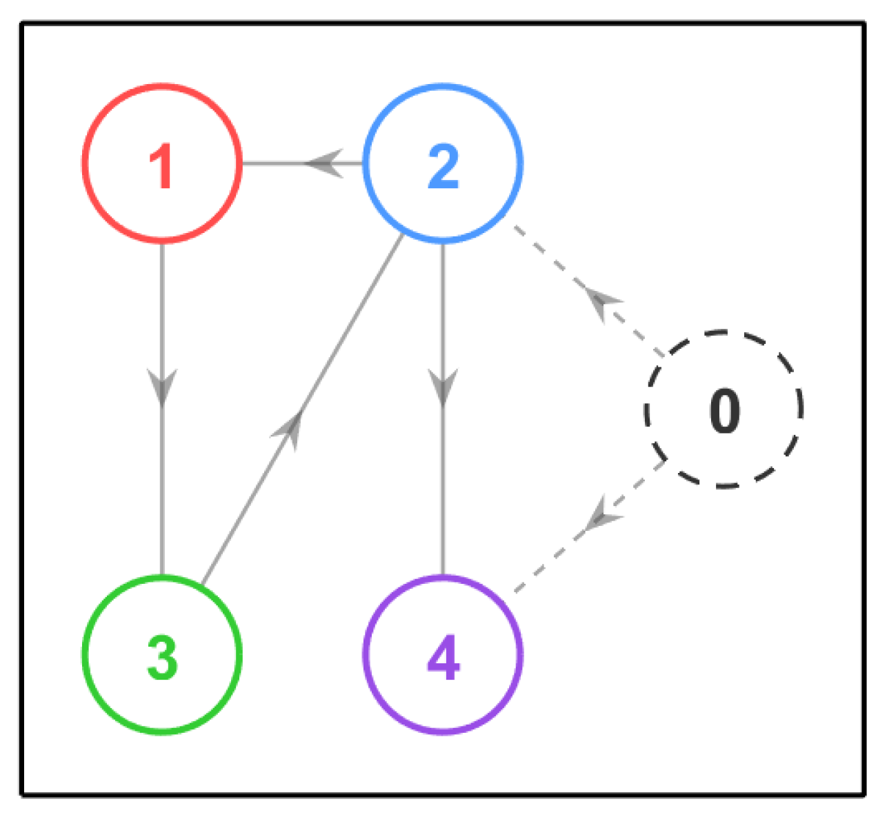
Figure 1 illustrates the invariant communication topology governing the network nodes of the FOCNNs. The node labeled as 0 corresponds to the virtual reference state, which indicates that the desired target information is directly accessible only by the second and fourth agents. Accordingly, the corresponding Laplacian matrix $\mathcal{L}$ and pinning gain matrix $\mathcal{B}$ are formulated as

$$\mathcal{L}=\left[\begin{array}{cccc}1& -1& 0& 0\\ 0& 1& -1& 0\\ -1& 0& 1& 0\\ 0& -1& 0& 1\end{array}\right],\mathcal{B}=\left[\begin{array}{cccc}0& 0& 0& 0\\ 0& 1& 0& 0\\ 0& 0& 0& 0\\ 0& 0& 0& 1\end{array}\right].$$

To verify the statement in Theorem 1, the selection of the control gain matrix is made as $\Gamma =\mathrm{diag}\{0.62,0.55,0.48,0.61\}$. By direct computation, the evaluation of the inequality yields $\rho =\parallel I_{Nm}-(\mathcal{L}+\mathcal{B})\otimes F\Gamma \parallel +\varpi \parallel (\mathcal{L}+\mathcal{B})\otimes F\Gamma \parallel =0.857<1$ under $\varpi =0.081$. Consequently, the validity of Theorem 1 is rigorously confirmed.

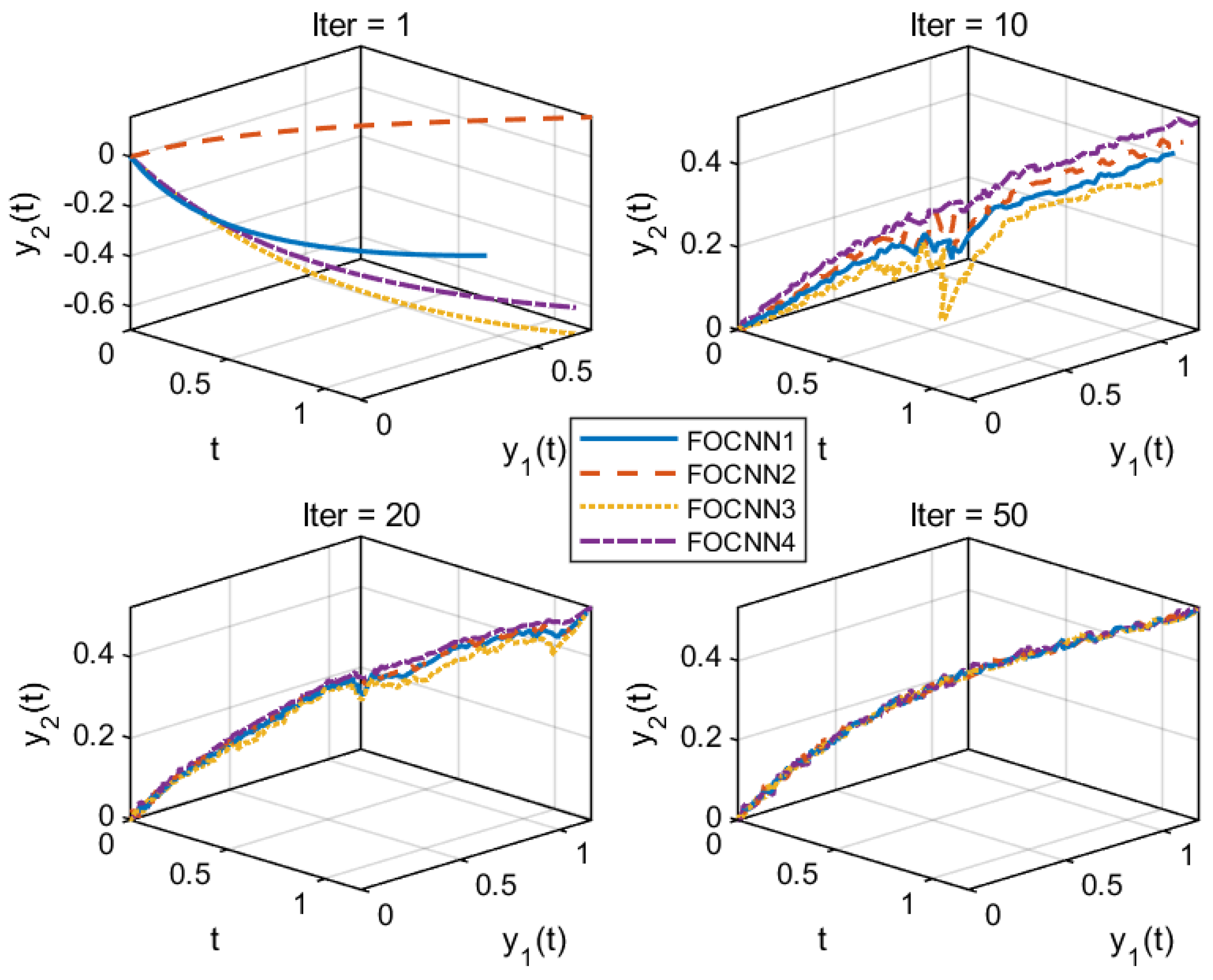
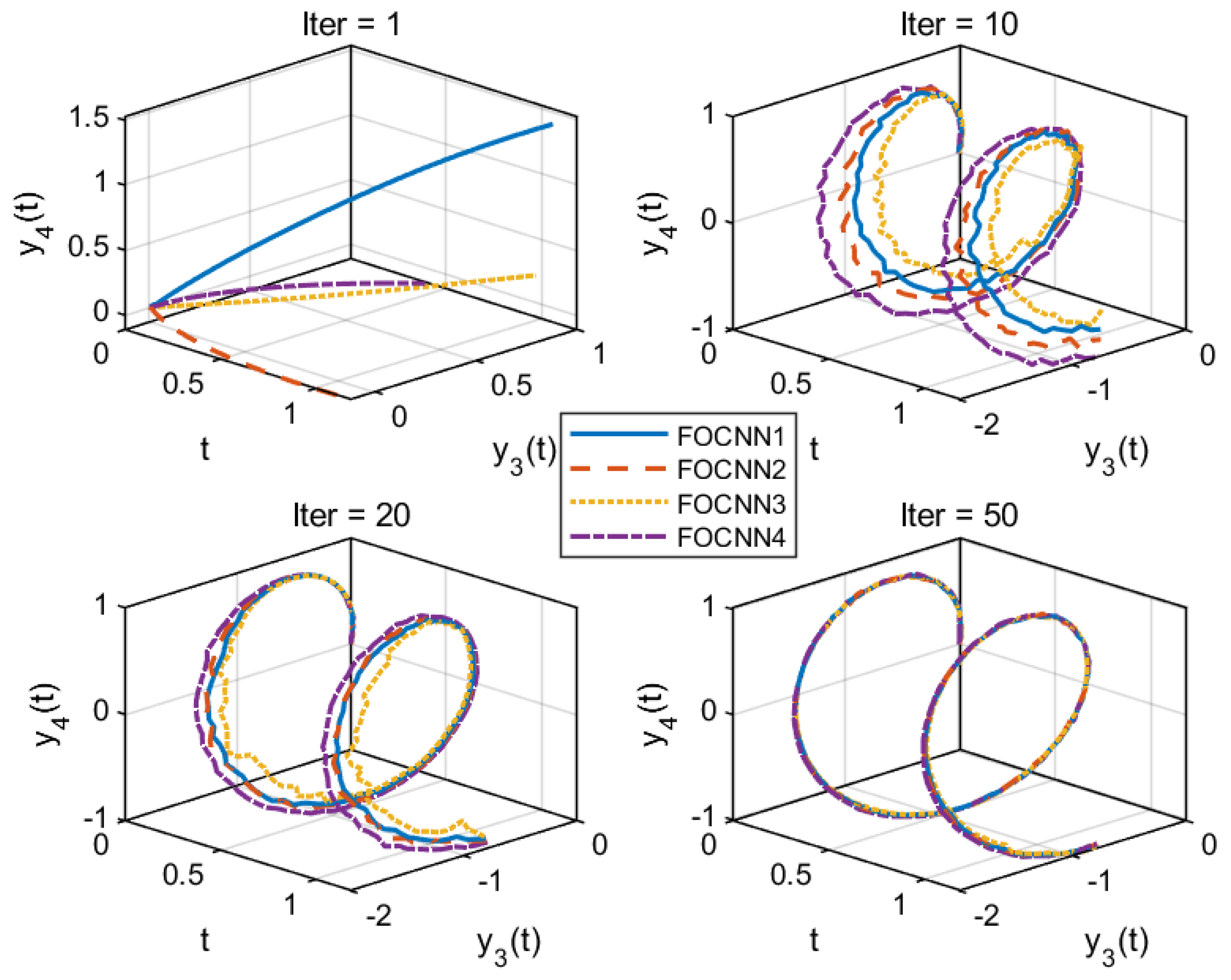
Figure 2 and Figure 3 provide a granular view of the $x\left(t\right)$ and $o\left(t\right)$ states, which generates the output $y_1\left(t\right),y_2\left(t\right)$ and $y_3\left(t\right),y_4\left(t\right)$, respectively. These profiles reveal that under the QSDILC protocol, the output synchronization error manifolds across the entire temporal horizon vanish within a finite number of iterations, effectively bridging the gap between actual plant responses and their target references.

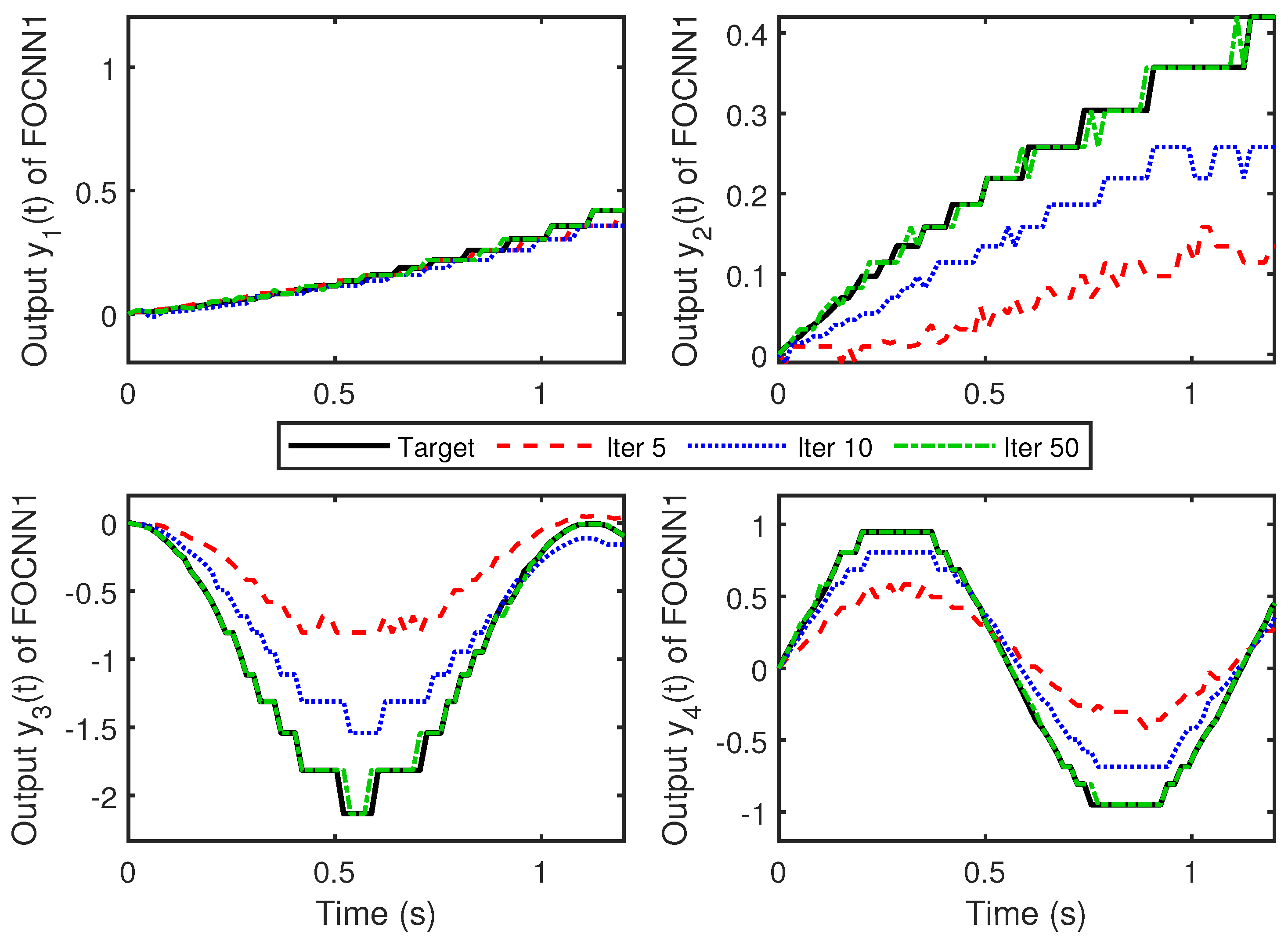
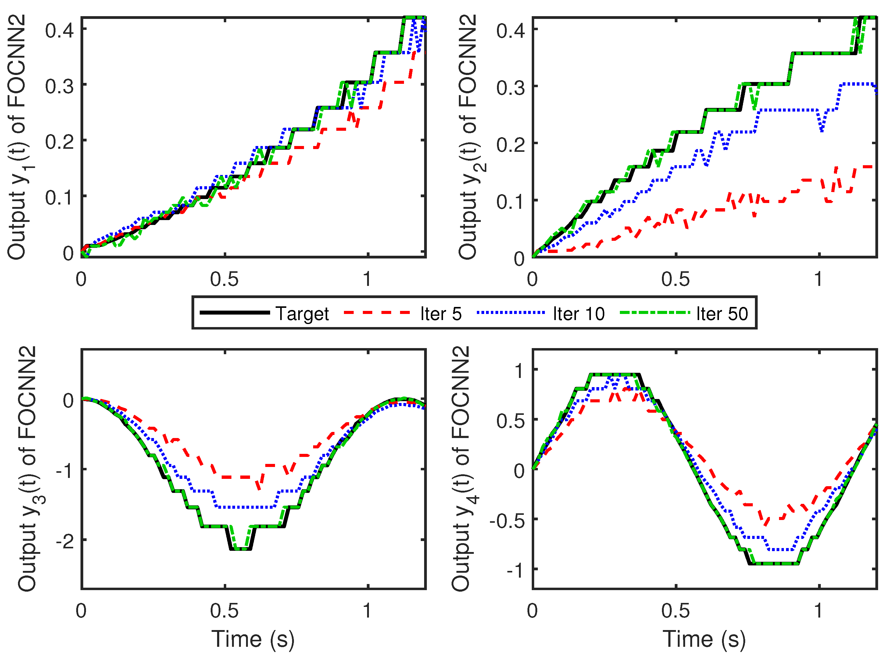
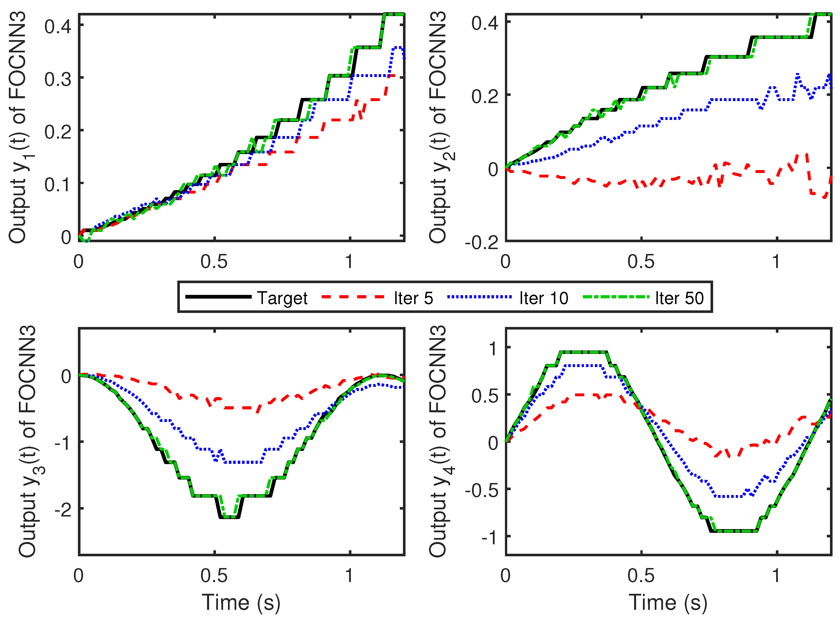
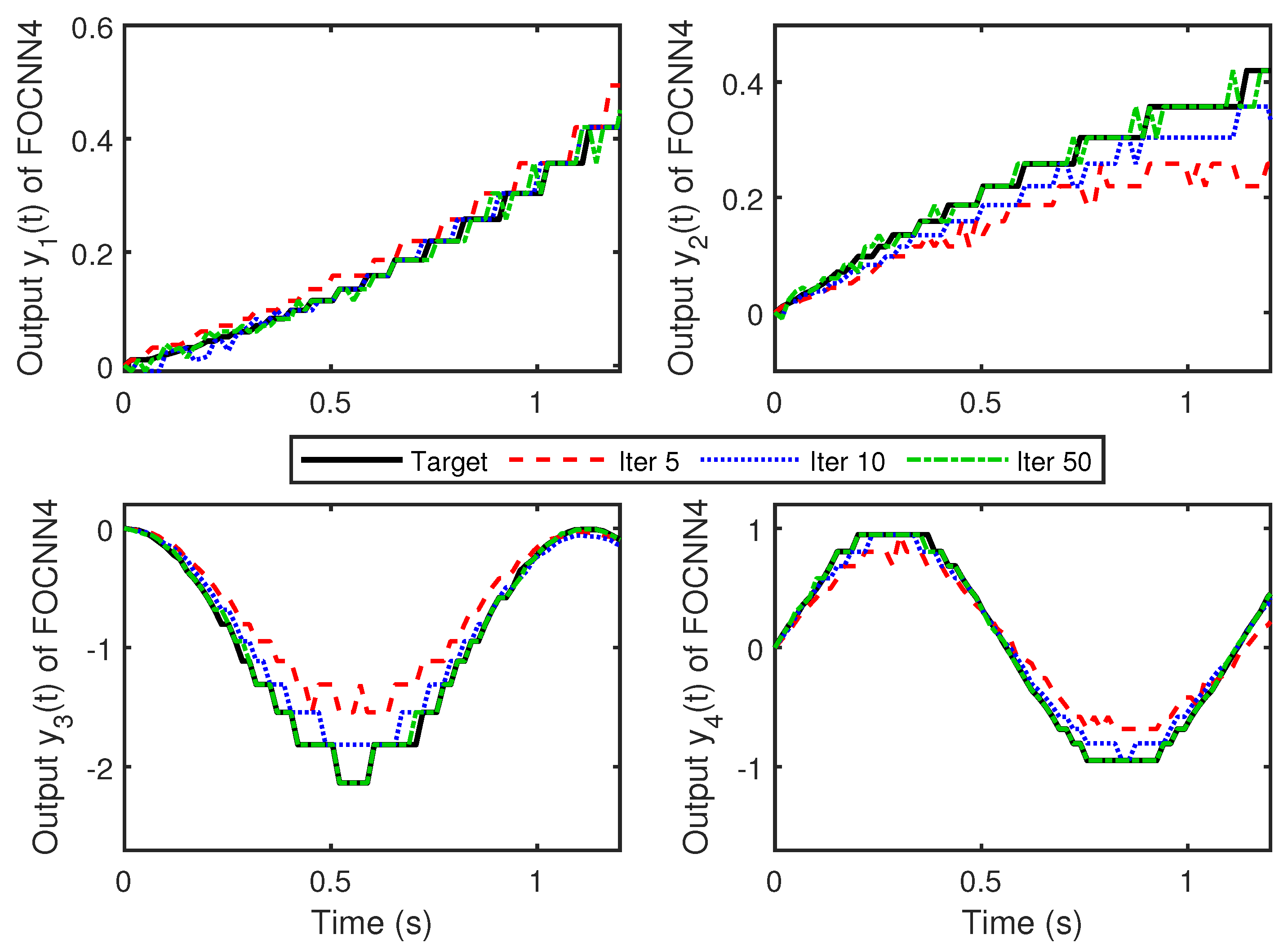
Figure 4, Figure 5, Figure 6 and Figure 7 illustrate the evolutionary performance of the proposed QSDILC protocol, demonstrating that both FOCNN-wise outputs and the multifaceted state deviations strictly converge to the target profiles along the iteration axis, achieving synchronization between the FOCNNs.

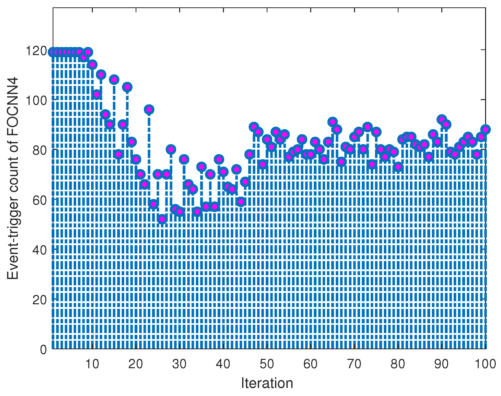
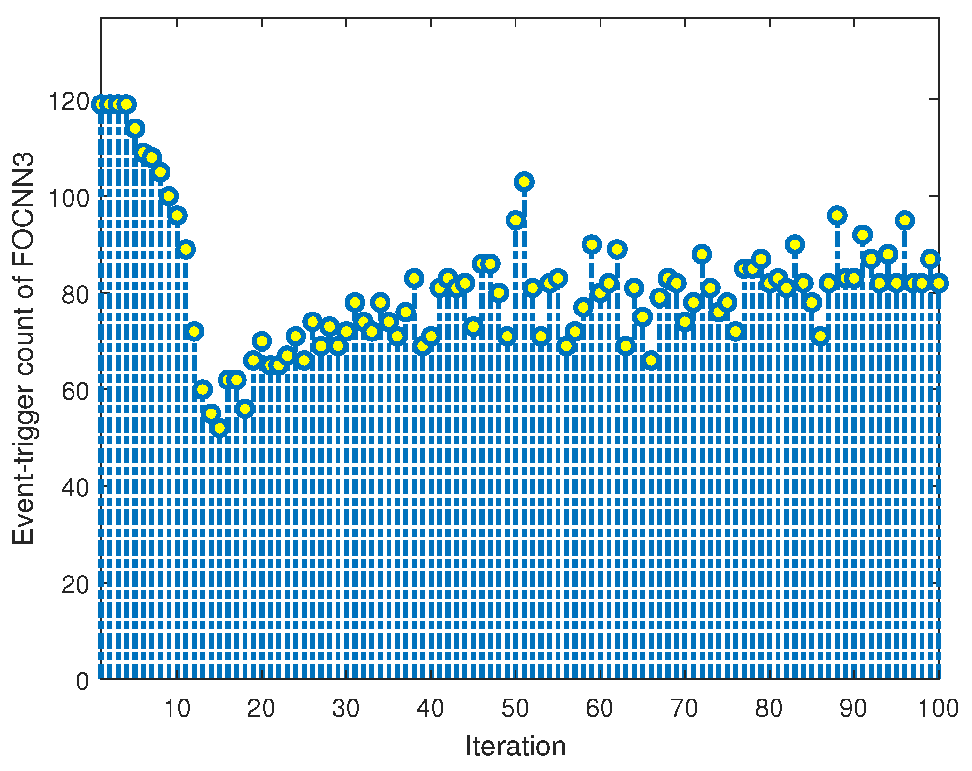
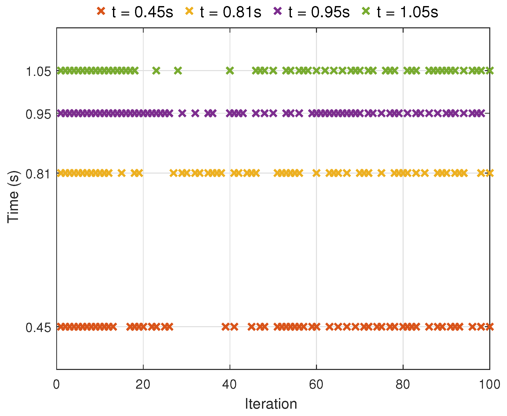
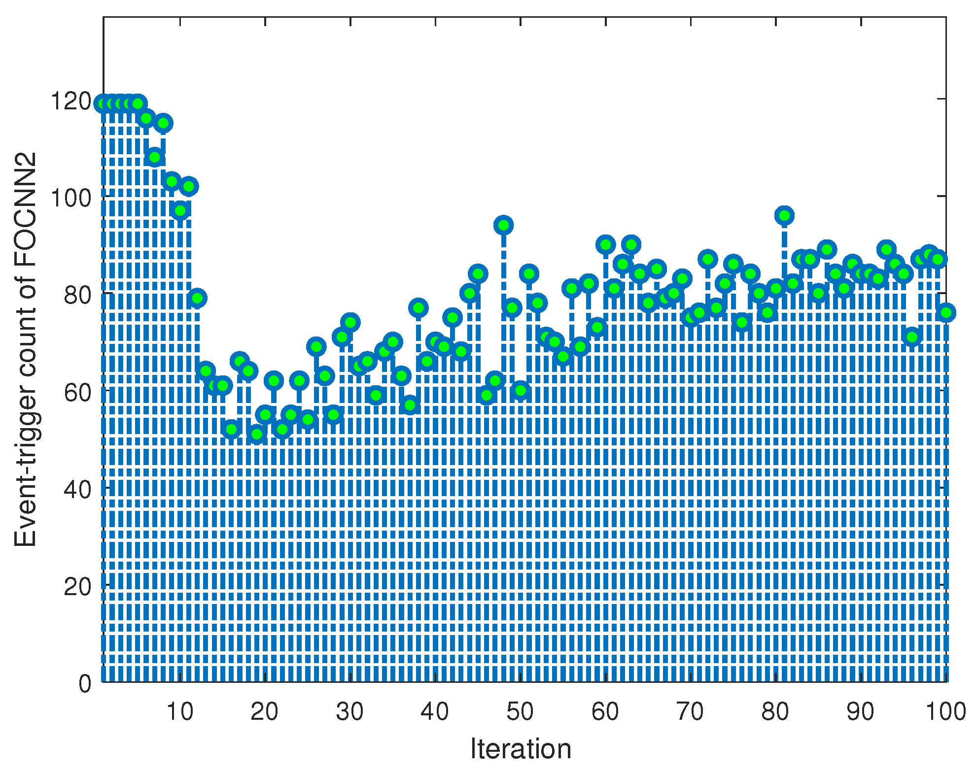
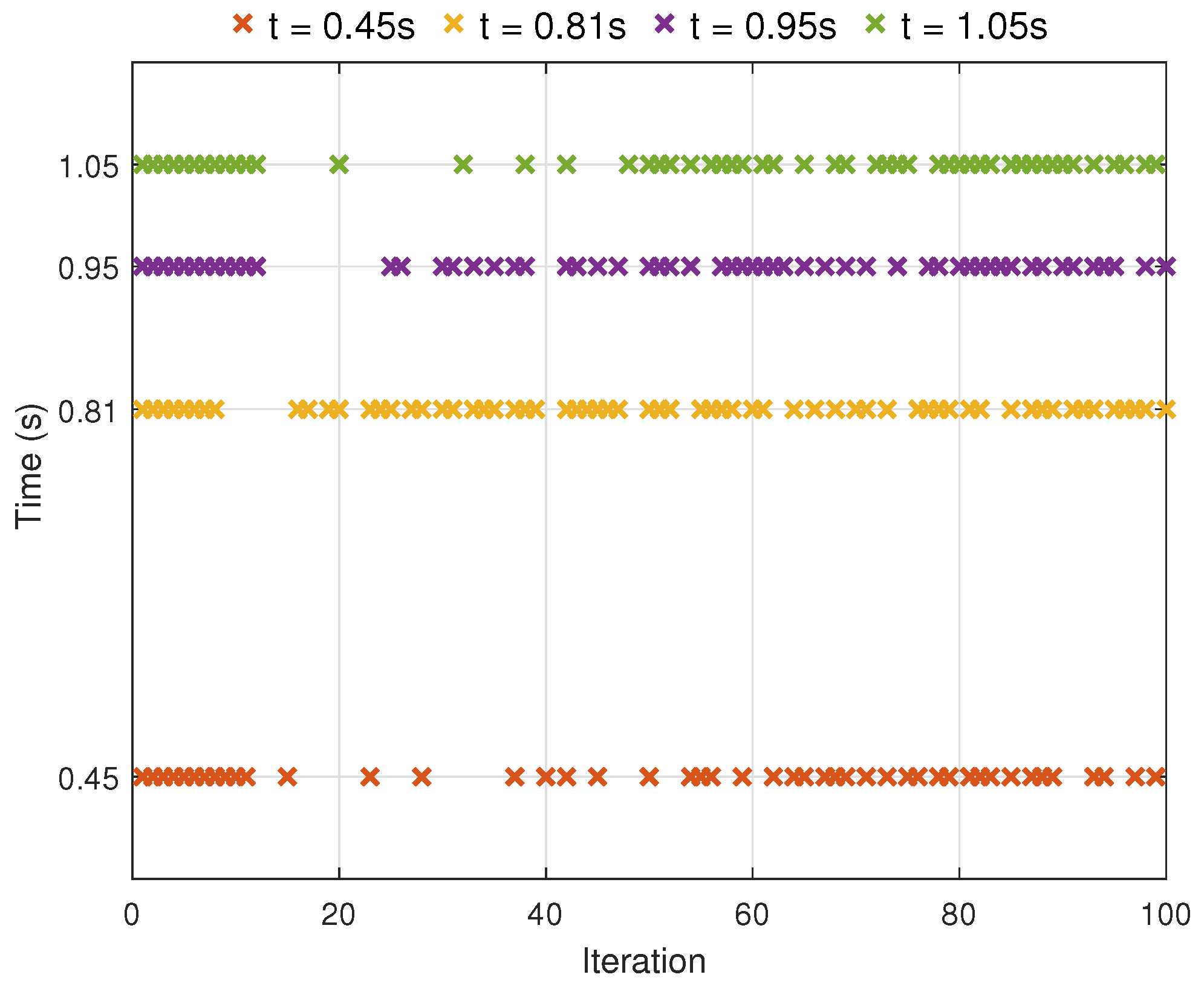
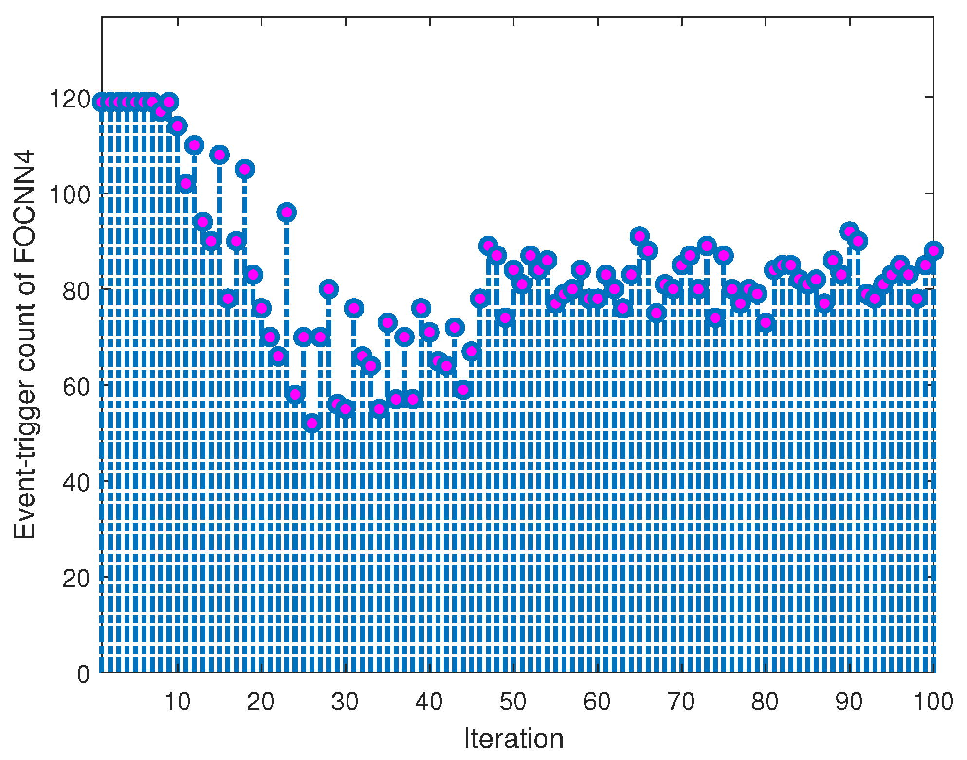
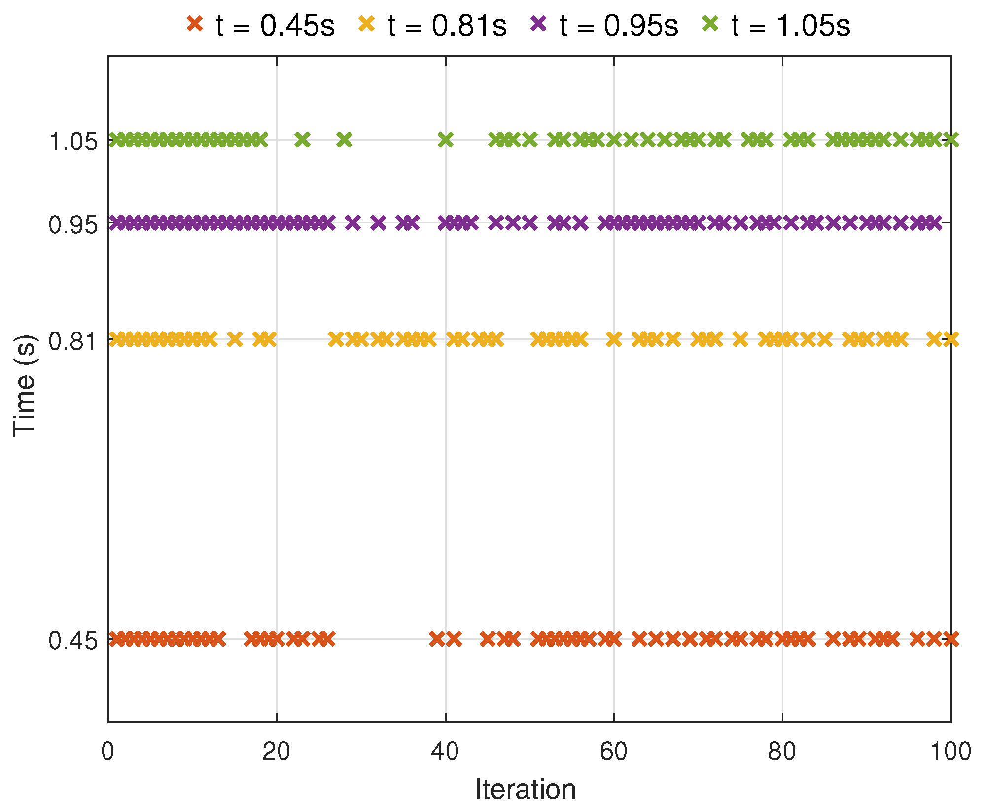
The comprehensive simulation results regarding the proposed event-triggered mechanisms for FOCNN1 through FOCNN4 are graphically visualized in Figure 8, Figure 9, Figure 10, Figure 11, Figure 12, Figure 13, Figure 14 and Figure 15. As clearly illustrated by the trigger occurrence counts, it is evident that a significant reduction in data transmission is successfully achieved as the iteration index increases. In particular, the event-triggering frequency is observed to gradually stabilize after a relatively short initial transient phase, thereby demonstrating the efficiency and reliability of the designed control strategy in practical scenarios.

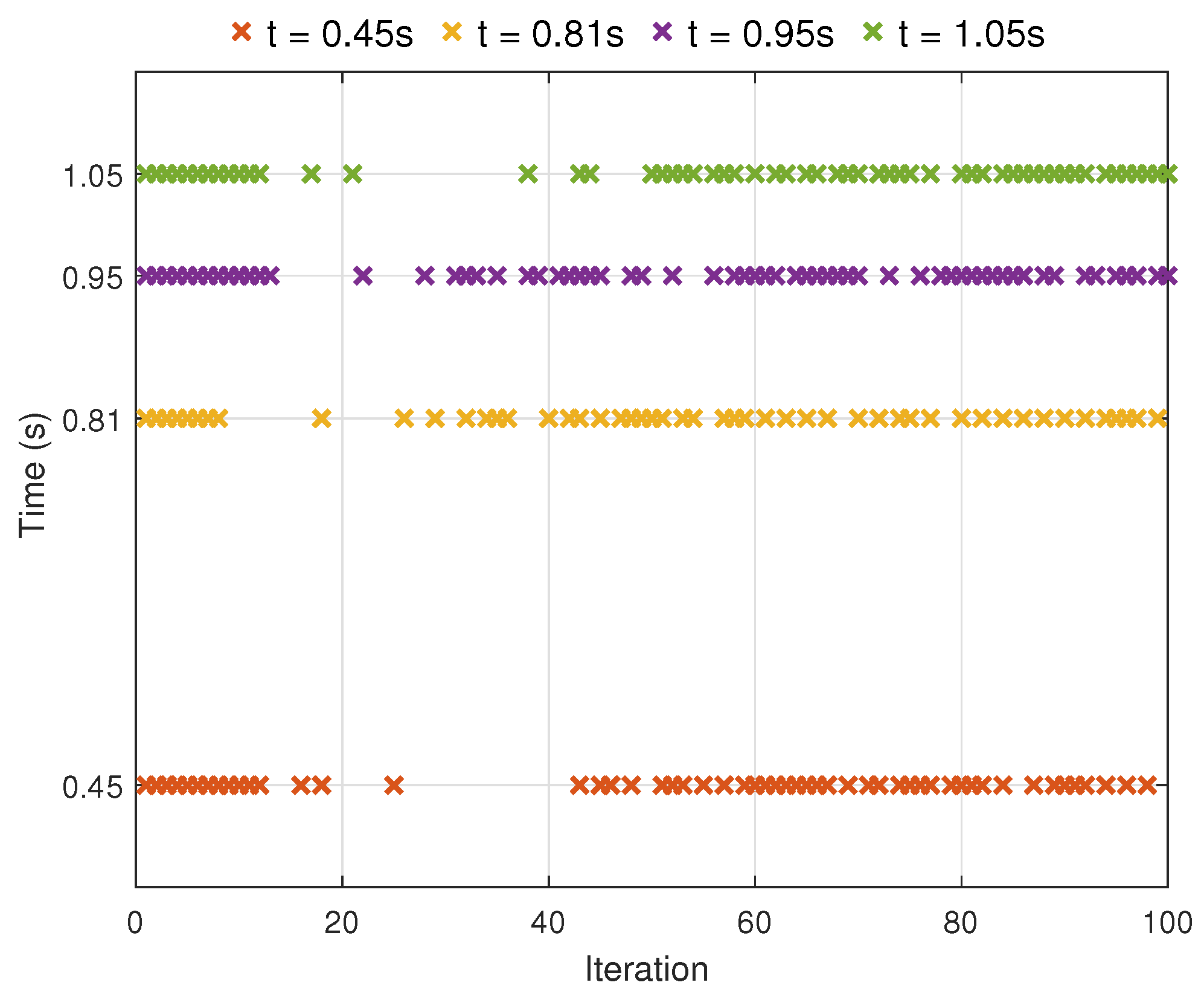
Furthermore, the event-triggered status across various time snapshots (t = 0.45 s, 0.81 s, 0.95 s, 1.05 s) is depicted to demonstrate the sparse execution of the QSDILC control law. It can be inferred from these trajectories that the communication overhead is effectively mitigated while the desired learning performance is maintained. Specifically, the consistent convergence patterns exhibited by all four FOCNN configurations validate the robustness of the proposed fractional-order learning scheme under the prescribed event-triggered condition.

The experimental results summarized in

Table 1. Sum of event-triggered counts for individual FOCNN nodes.

	Actuated Triggering Counts	Theoretical Maximum Times	Communication Ratio
FOCNN1	8325	12,000	69.38%
FOCNN2	7875	12,000	65.63%
FOCNN3	8095	12,000	67.46%
FOCNN4	8305	12,000	69.21%

demonstrate the efficacy of the proposed EEA-driven event-triggered mechanism across four FOCNN modules, revealing a significant reduction in communication overhead. By achieving actual triggering counts of 8325, 7875, 8095, and 8305 against a theoretical maximum of 12,000, the framework successfully reduces communication overhead by 30.62% for FOCNN1, 34.37% for FOCNN2, 32.54% for FOCNN3, and 30.79% for FOCNN4, respectively. This empirical evidence validates the FOCNNs’s ability to maintain computational performance while substantially mitigating the communication burden, a critical factor for the scalability of decentralized or resource-constrained neural architectures.

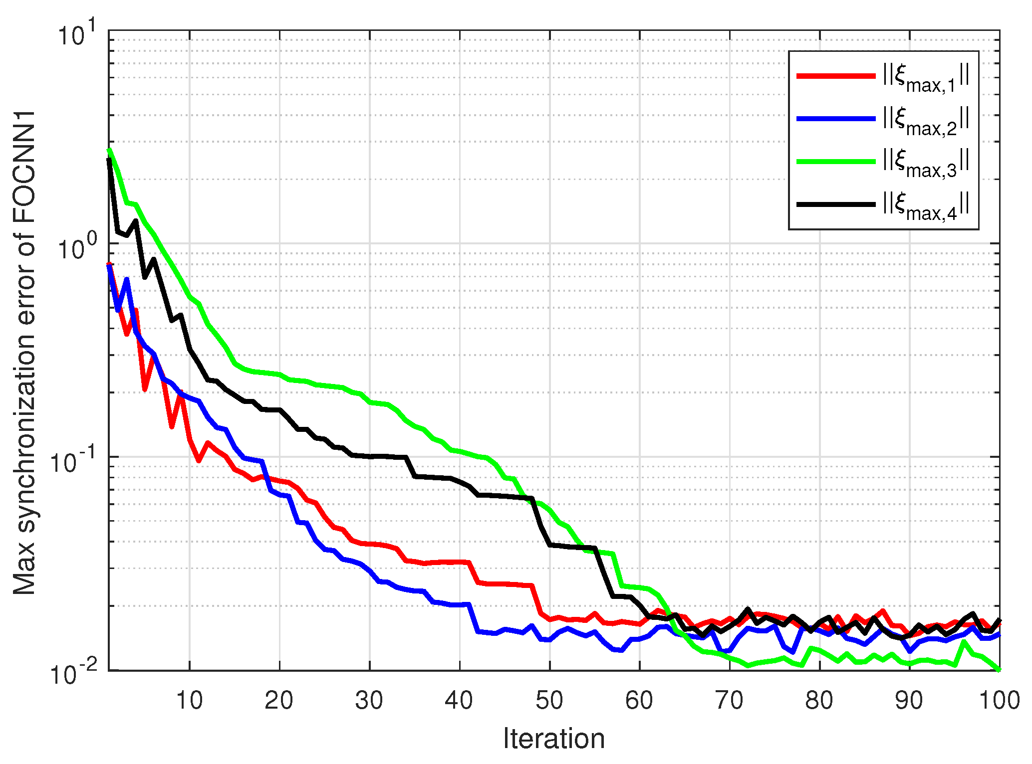
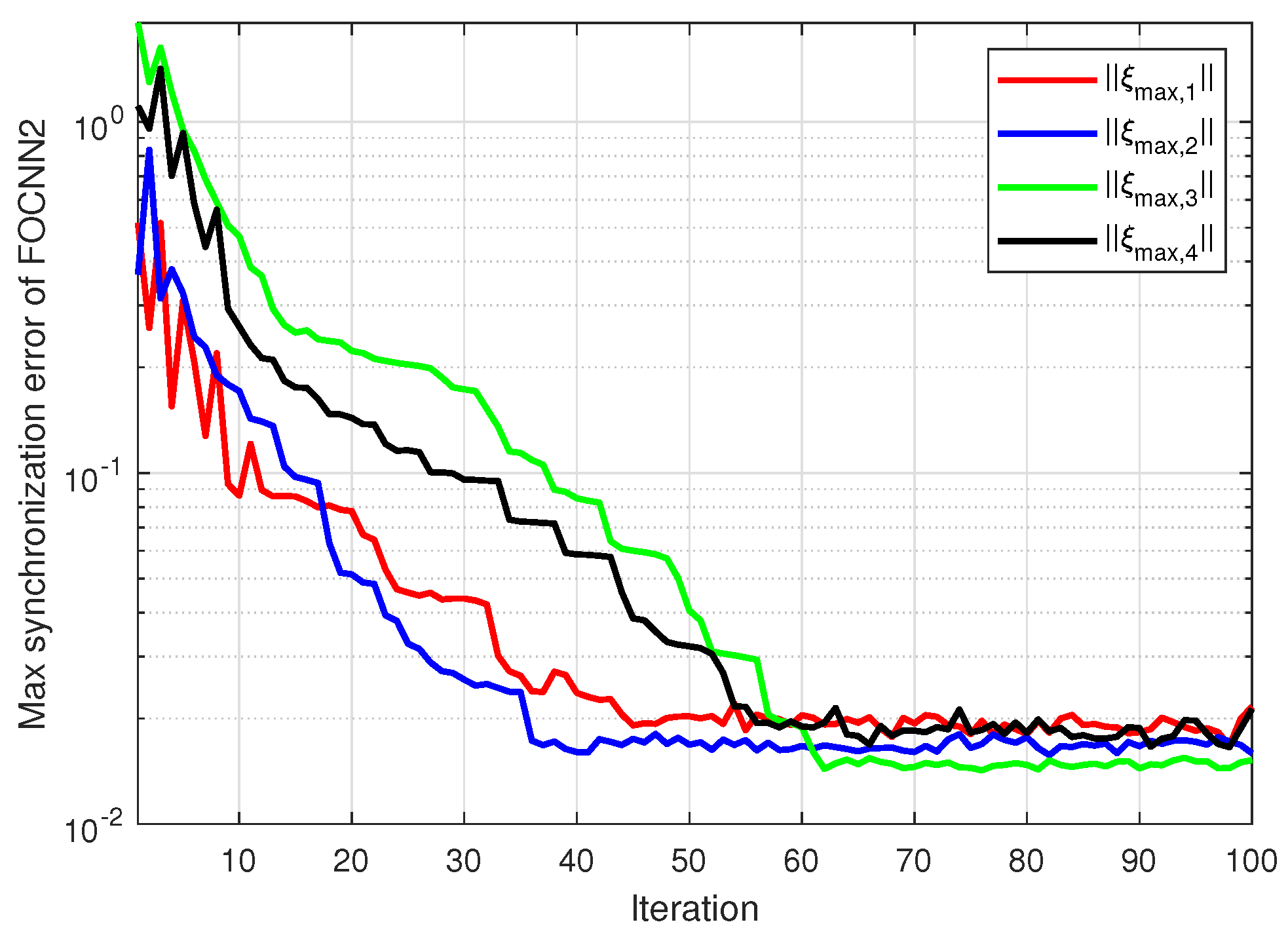
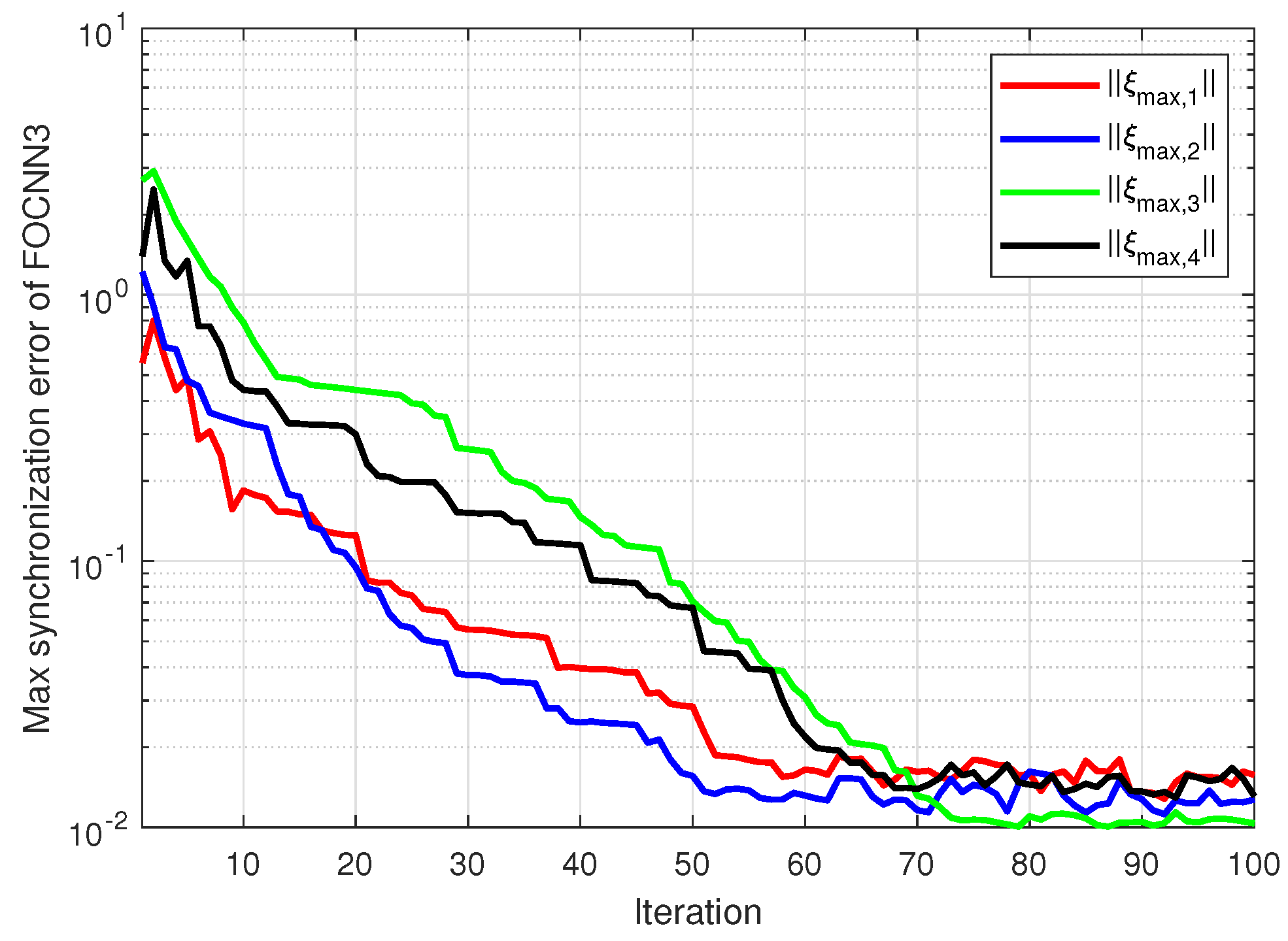
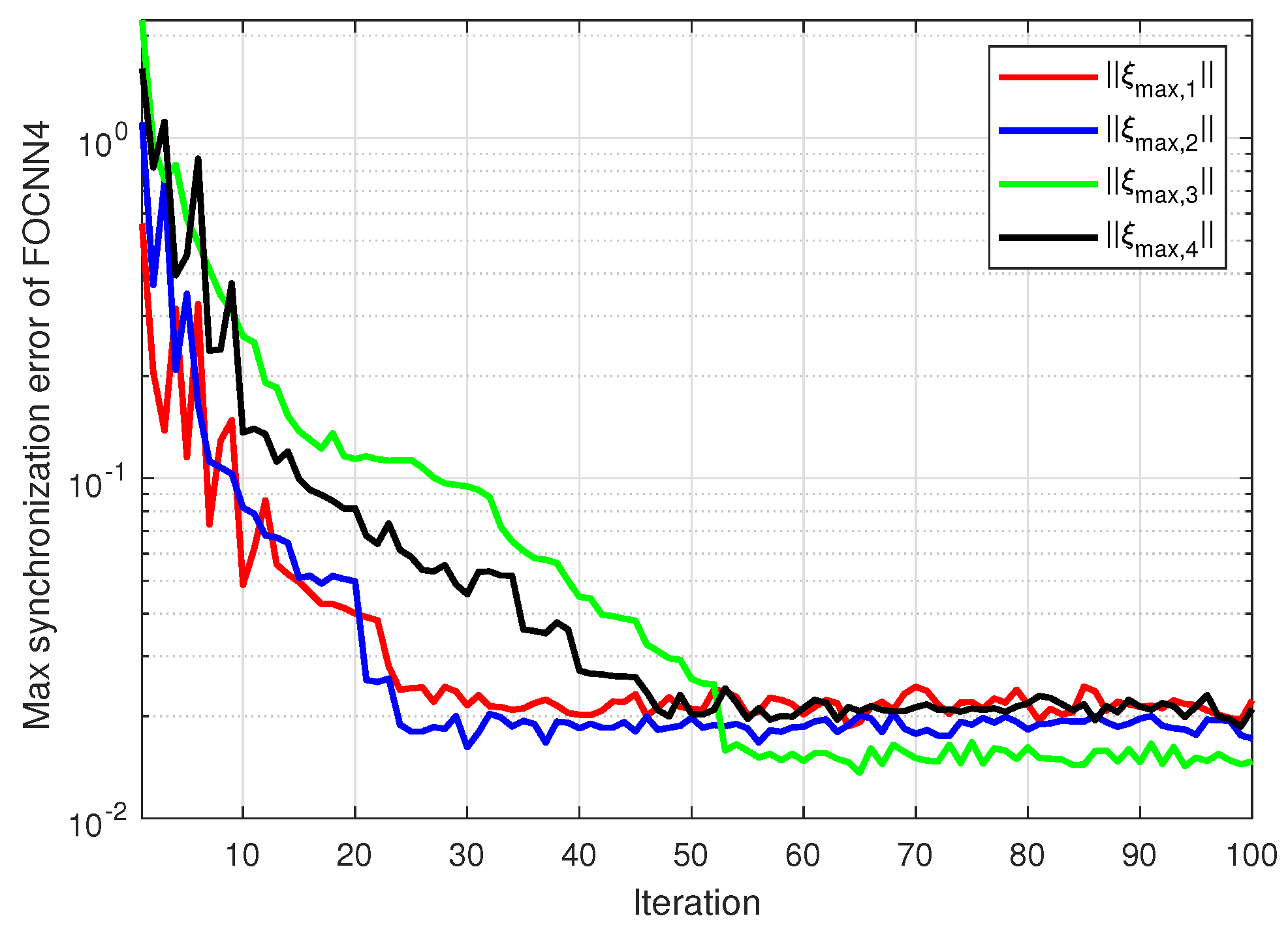
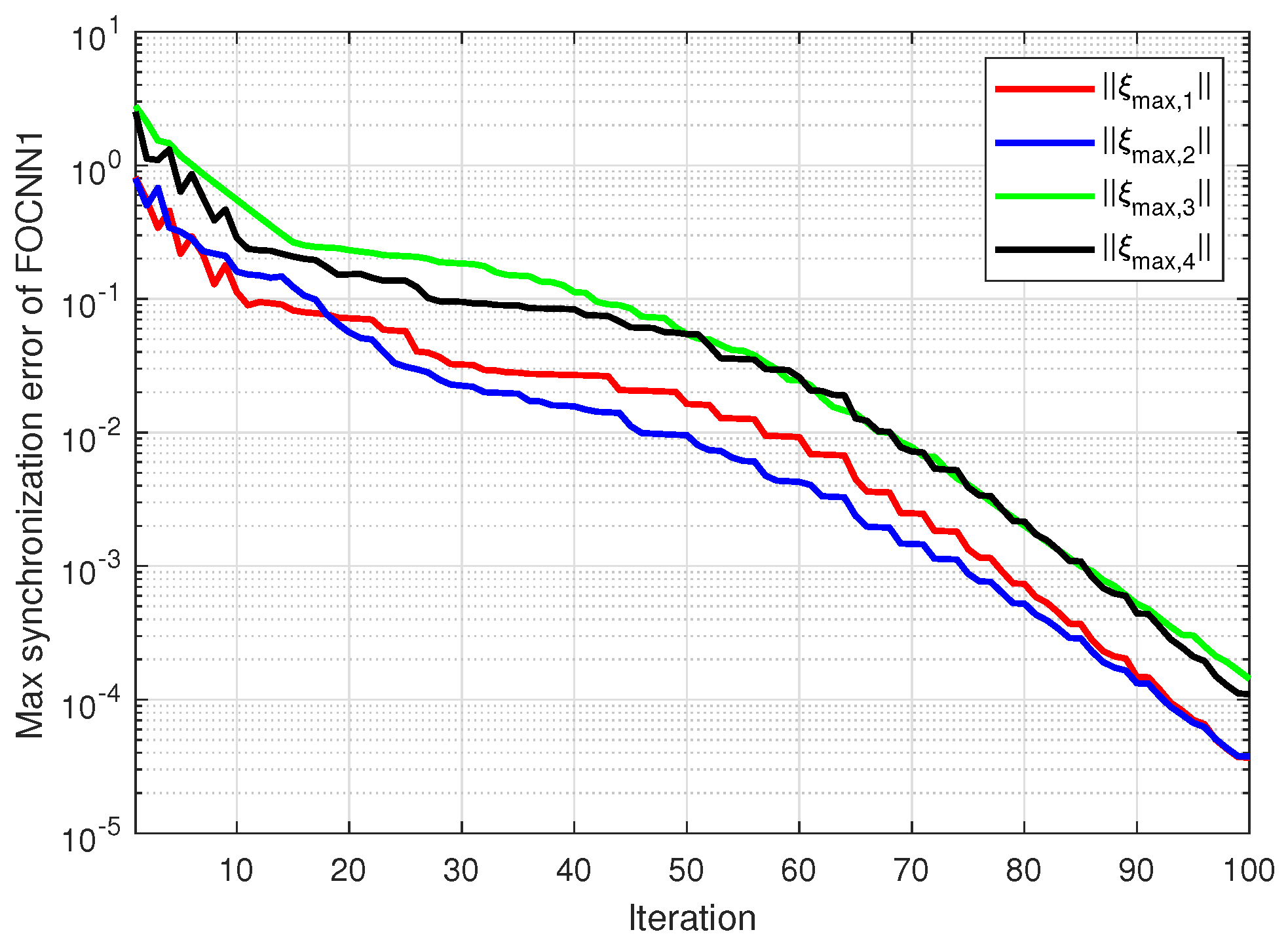
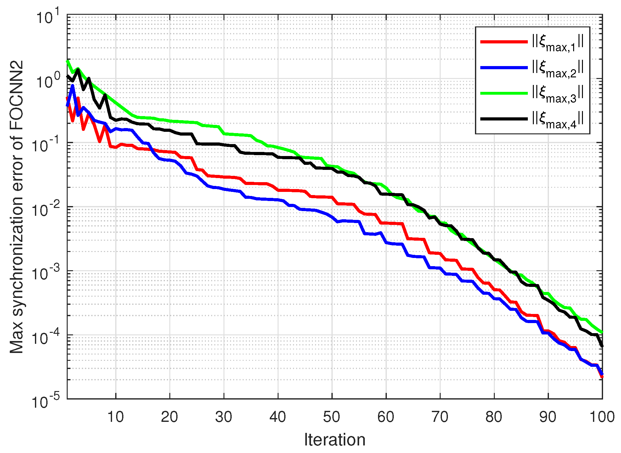
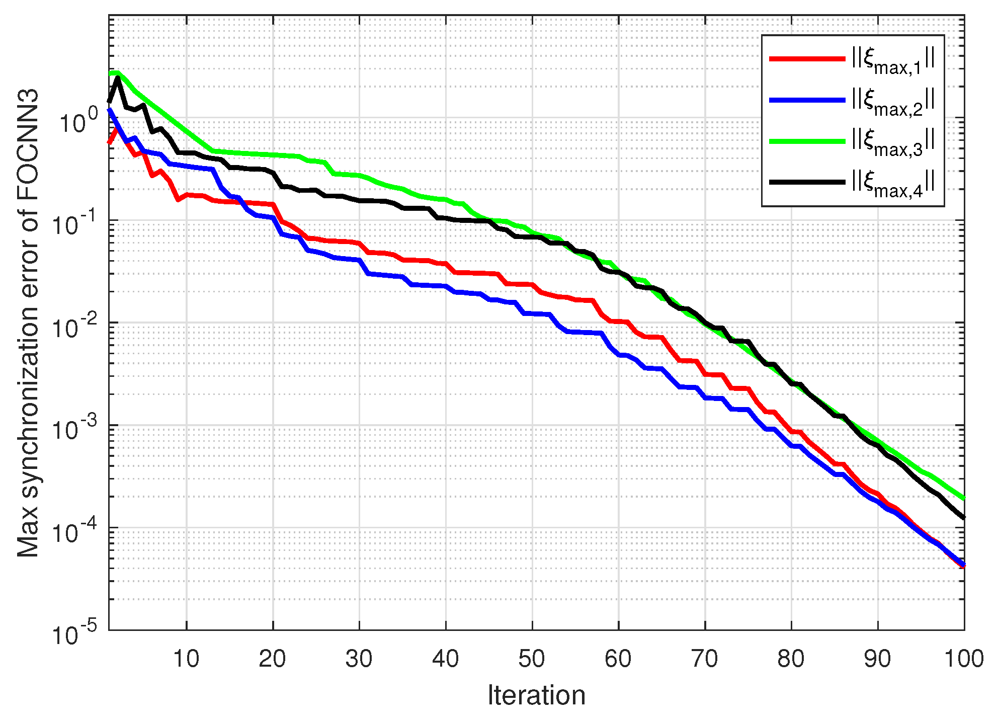
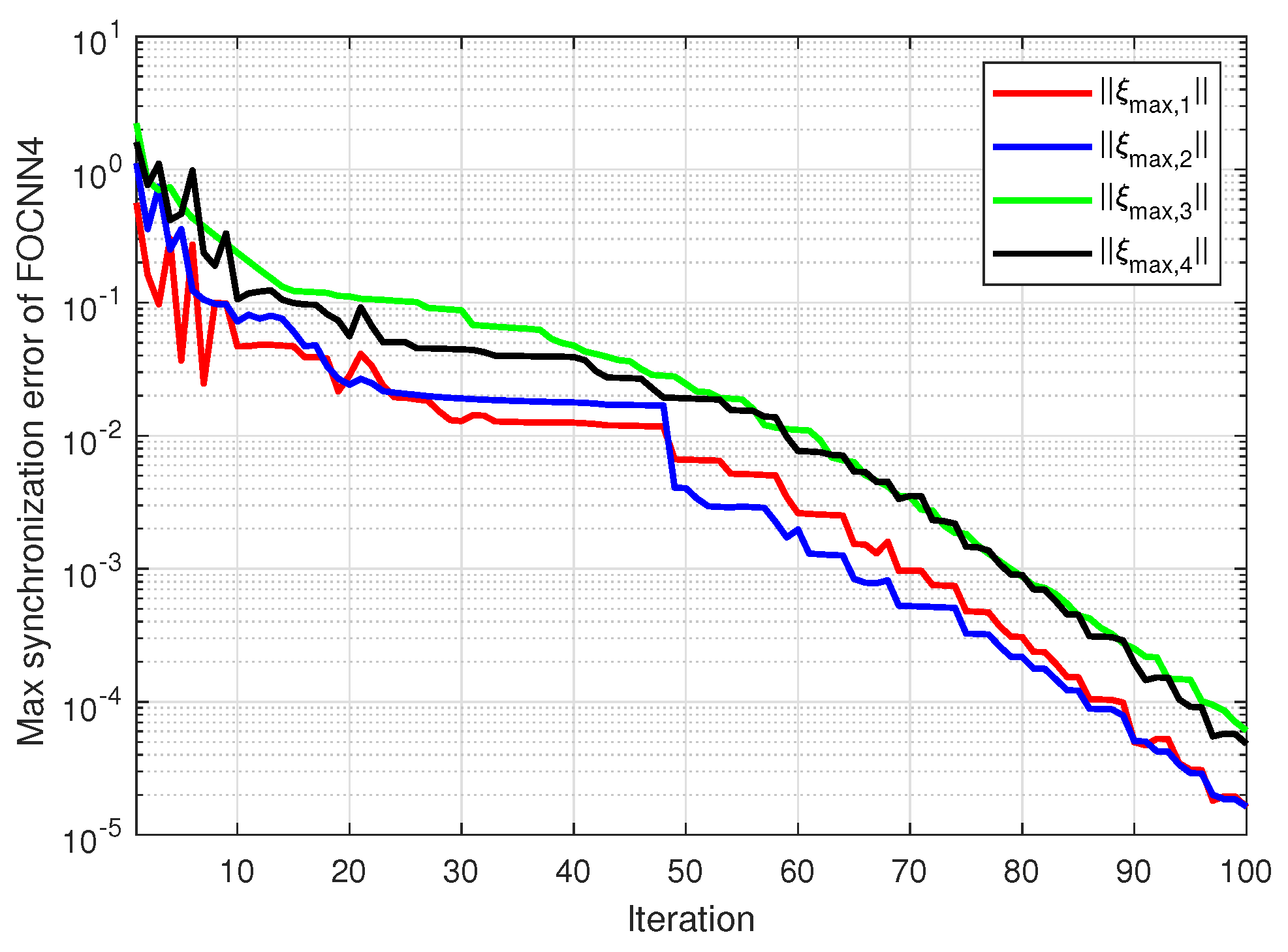
The peak output-synchronization error profiles for FOCNN1 through FOCNN4, operating under the proposed QSDILC protocol, are illustrated in Figure 16, Figure 17, Figure 18 and Figure 19. These trajectories specifically highlight the FOCNNs’ resilience to quantization effects integrated within the sampled-data framework. It is observed that despite the precision constraints imposed by the quantizer, a consistent downward trend is maintained across all iterations. While the introduction of quantization errors inevitably leads to localized oscillations in the initial phase, the errors successfully converge to a predefined neighborhood of the origin. This validates that the QSDILC protocol effectively compensates for information loss during the quantization process, ensuring that high-precision learning performance is preserved even under significant data compression.

A comparative analysis between Figure 16, Figure 17, Figure 18 and Figure 19 and Figure 20, Figure 21, Figure 22 and Figure 23 reveals the distinct impact of the quantization process within the QSDILC framework. In the absence of quantization, the maximum output synchronization errors exhibit a smoother and more rapid decay, eventually reaching a significantly lower steady-state precision. Conversely, when the QSDILC protocol is employed with quantization effects, the convergence trajectories are characterized by localized fluctuations and a slightly higher error floor, which is attributed to the inherent information loss and mapping errors of the quantizer. The advantage of the unquantized scheme lies in its superior synchronization accuracy and faster convergence rate, making it suitable for high-precision tasks. However, its disadvantage involves a heavy reliance on high-bandwidth communication to transmit continuous-valued signals. In contrast, the quantized QSDILC scheme, while sacrificing a degree of precision, offers the critical advantage of significantly reduced communication overhead and enhanced resource efficiency, which is indispensable for practical networked neural systems with bandwidth constraints.

7. Conclusions

In this research, the output synchronization target inherent in FOCNNs with time delays has been comprehensively addressed. The QSDILC protocol has been successfully formulated, through which the constraints of limited communication bandwidth and high computational costs have been effectively mitigated. Furthermore, the EEA-based event-triggered mechanism has been orchestrated to prune redundant iterations, ensuring that transmission efficiency has been significantly optimized without compromising convergence stability. The theoretical feasibility of this framework has been rigorously established via the properties of fractional calculus together with the contraction mapping theorem. Finally, numerical verifications have convincingly highlighted the realistic advantages of the synthesized QSDILC strategy under the EEA triggering law, whereby a substantial reduction in communication overhead and computational burden has been achieved for large-scale FOCNN implementations.

References

1. Chang, S.; Wang, C.; Ma, Y. Dual event-triggered intermittent synchronization for complex dynamic networks with time delay under hybrid attacks. Inf. Sci. 2026, 754, 123664. [Google Scholar] [CrossRef] [Scilit]
2. Kumar, R. A stable framework-based modeling of the complex dynamical system using a double context layered with self-weighted output feedback loop Elman recurrent neural network. Inf. Sci. 2025, 712, 122132. [Google Scholar] [CrossRef] [Scilit]
3. Tang, Z.; Liu, X. Synchronization of directly coupled complex networks with multiweights and multiple delays. Chaos Solitons Fractals 2024, 188, 115569. [Google Scholar] [CrossRef] [Scilit]
4. Luo, S.; Ye, D. Cluster consensus control of linear multiagent systems under directed topology with general partition. IEEE Trans. Autom. Control 2021, 67, 1929–1936. [Google Scholar] [CrossRef] [Scilit]
5. Gu, H.; Liu, K.; Lü, J. Adaptive PI control for synchronization of complex networks with stochastic coupling and nonlinear dynamics. IEEE Trans. Circuits Syst. I Regul. Pap. 2020, 67, 5268–5280. [Google Scholar] [CrossRef] [Scilit]
6. Meyer-Bäse, A.; Botella, G.; Rybarska-Rusinek, L. Stochastic stability analysis of competitive neural networks with different time-scales. Neurocomputing 2013, 118, 115–118. [Google Scholar] [CrossRef] [Scilit]
7. Yang, Y.; Liu, Y. Global exponential convergence and synchronization for exponential numerical competitive neural networks with different time scales and fuzzy logic. Proc. Inst. Mech. Eng. Part C J. Mech. Eng. Sci. 2024, 238, 18. [Google Scholar] [CrossRef] [Scilit]
8. Zhou, X.; Wang, H.; Wang, K.; Tian, Y. Quantized iterative learning control for singular nonlinear fractional-order time-delay multi-agent systems with iteration-varying reference trajectories and switching topologies. Commun. Nonlinear Sci. Numer. Simul. 2023, 125, 107359. [Google Scholar] [CrossRef] [Scilit]
9. Wang, H.; Yu, Y.; Wen, G. Stability analysis of fractional-order Hopfield neural networks with time delays. Neural Netw. 2014, 55, 98–109. [Google Scholar] [CrossRef] [Scilit] [PubMed]
10. Pratap, A.; Raja, R.; Agarwal, R.P.; Cao, J. Stability analysis and robust synchronization of fractional-order competitive neural networks with different time scales and impulsive perturbations. Int. J. Adapt. Control Signal Process. 2019, 33, 1635–1660. [Google Scholar] [CrossRef] [Scilit]
11. Wang, S.; Jian, J. Predefined-time synchronization of fractional-order memristive competitive neural networks with time-varying delays. Chaos Solitons Fractals 2023, 174, 113790. [Google Scholar] [CrossRef] [Scilit]
12. Wang, S.; Jian, J. Predefined-time synchronization of incommensurate fractional-order competitive neural networks with time-varying delays. Chaos Solitons Fractals 2023, 177, 114216. [Google Scholar] [CrossRef] [Scilit]
13. Shen, J.; Cao, J. Finite-time synchronization of coupled neural networks via discontinuous controllers. Cogn. Neurodyn. 2011, 5, 373–385. [Google Scholar] [CrossRef] [Scilit] [PubMed]
14. Zhuang, Z.; González, R.A.; Tao, H.; Paszke, W.; Oomen, T. Data-enabled iterative learning control: A zero-sum game design for time-scale-varying tasks. Automatica 2026, 185, 112781. [Google Scholar] [CrossRef] [Scilit]
15. Wang, W.; Meng, D.; Zhang, L.; Cai, K. Design and experimental validation of adaptive iterative learning control for nonlinear vehicular platoons. Automatica 2026, 183, 112680. [Google Scholar] [CrossRef] [Scilit]
16. Cao, X.; Fečkan, M.; Shen, D.; Wang, J. Iterative learning control for multi-agent systems with impulsive consensus tracking. Nonlinear Anal. Model. Control 2021, 26, 130–150. [Google Scholar] [CrossRef] [Scilit]
17. Han, T.; Zhou, X.; Zhang, S.; Qiu, A. Consensus synchronization via quantized iterative learning for coupled fractional-order time-delayed competitive neural networks with input sharing. Neural Netw. 2025, 189, 107569. [Google Scholar] [CrossRef] [Scilit] [PubMed]
18. Zhou, X.; Wang, H.; Tian, Y.; Dai, X. Consensus tracking via quantized iterative learning control for singular nonlinear multi-agent systems with state time-delay and initial state error. Nonlinear Dyn. 2021, 103, 2701–2719. [Google Scholar] [CrossRef] [Scilit]
19. Karaki, B.J.; Mahmoud, M.S. Event-triggered leader-following consensus for a class of nonlinear multiagent systems with time-varying delay. Int. J. Robust Nonlinear Control 2022, 32, 3314–3333. [Google Scholar] [CrossRef] [Scilit]
20. Hui, Y.; Meng, D.; Chi, R.; Cai, K. Sampled-data adaptive iterative learning control for uncertain nonlinear systems. IEEE Trans. Syst. Man Cybern. Syst. 2024, 54, 4568–4578. [Google Scholar] [CrossRef] [Scilit]
21. Zhang, T.; Li, J. Event-triggered iterative learning control for multi-agent systems with quantization. Asian J. Control 2018, 20, 1088–1101. [Google Scholar] [CrossRef] [Scilit]
22. Wang, L.; Zhang, G. Event-triggered iterative learning control for perfect consensus tracking of non-identical fractional order multi-agent systems. Int. J. Control Autom. Syst. 2021, 19, 1426–1442. [Google Scholar] [CrossRef] [Scilit]
23. Yu, Q.; Fan, Z.; Bu, X.; Hou, Z. Event-triggered based predictive iterative learning control with random packet loss compensation for nonlinear networked systems. ISA Trans. 2024, 148, 169–181. [Google Scholar] [CrossRef] [Scilit] [PubMed]
24. Povstenko, Y. Essentials of Fractional Calculus. In Fractional Thermoelasticity; Springer: Cham, Switzerland, 2024; pp. 1–19. [Google Scholar]
25. Haubold, H.J.; Mathai, A.M.; Saxena, R.K. Mittag-Leffler functions and their applications. J. Appl. Math. 2011, 2011, 298628. [Google Scholar] [CrossRef] [Scilit]
26. Saxena, R.; Kalla, S.L. On the solutions of certain fractional kinetic equations. Appl. Math. Comput. 2008, 199, 504–511. [Google Scholar] [CrossRef] [Scilit]
27. Li, Y.; Chen, Y.; Ahn, H.S. Fractional-order iterative learning control for fractional-order linear systems. Asian J. Control 2011, 13, 54–63. [Google Scholar] [CrossRef] [Scilit]
28. Diethelm, K.; Ford, N.J. Analysis of fractional differential equations. J. Math. Anal. Appl. 2002, 265, 229–248. [Google Scholar] [CrossRef] [Scilit]
29. Fu, M.; Xie, L. The sector bound approach to quantized feedback control. IEEE Trans. Autom. Control 2005, 50, 1698–1711. [Google Scholar] [CrossRef] [Scilit]
Figure 1. Invariant network topology governing the communication among neural units.
Fractalfract 10 00606 g001
Figure 2. Evolution of the output of x ( t ) in three-dimensional space at different iterations.
Fractalfract 10 00606 g002
Figure 3. Evolution of the output of o ( t ) in three-dimensional space at different iterations.
Fractalfract 10 00606 g003
Figure 4. Output-synchronization evolution curves concerning the first FOCNN node.
Fractalfract 10 00606 g004
Figure 5. Output-synchronization evolution curves concerning the second FOCNN node.
Fractalfract 10 00606 g005
Figure 6. Output-synchronization evolution curves concerning the third FOCNN node.
Fractalfract 10 00606 g006
Figure 7. Output-synchronization evolution curves concerning the fourth FOCNN node.
Fractalfract 10 00606 g007
Figure 8. The number of trigger occurrences of FOCNN 1.
Fractalfract 10 00606 g008
Figure 9. Event-triggered status of FOCNN 1.
Fractalfract 10 00606 g009
Figure 10. The number of trigger occurrences of FOCNN 2.
Fractalfract 10 00606 g010
Figure 11. Event-triggered status of FOCNN 2.
Fractalfract 10 00606 g011
Figure 12. The number of trigger occurrences of FOCNN 3.
Fractalfract 10 00606 g012
Figure 13. Event-triggered status of FOCNN 3.
Fractalfract 10 00606 g013
Figure 14. The number of trigger occurrences of FOCNN 4.
Fractalfract 10 00606 g014
Figure 15. Event-triggered status of FOCNN 4.
Fractalfract 10 00606 g015
Figure 16. The evolution of maximum errors for FOCNN1 with quantification.
Fractalfract 10 00606 g016
Figure 17. The evolution of maximum errors for FOCNN2 with quantification.
Fractalfract 10 00606 g017
Figure 18. The evolution of maximum errors for FOCNN3 with quantification.
Fractalfract 10 00606 g018
Figure 19. The evolution of maximum errors for FOCNN4 with quantification.
Fractalfract 10 00606 g019
Figure 20. Transient behaviors of maximum tracking errors for FOCNN1.
Fractalfract 10 00606 g020
Figure 21. Transient behaviors of maximum tracking errors for FOCNN2.
Fractalfract 10 00606 g021
Figure 22. Transient behaviors of maximum tracking errors for FOCNN3.
Fractalfract 10 00606 g022
Figure 23. Transient behaviors of maximum tracking errors for FOCNN4.
Fractalfract 10 00606 g023