Optical Soliton Solutions for Fractal Modified Zakharov–Kuznetsov Equation on Cantor Sets and Modulation Instability Analysis

Abstract

In this paper, the new fractal modified Zakharov–Kuznetsov equation (fmZKe) defined on Cantor sets is investigated. The fmZKe is a non-differentiable model that arises naturally in mathematical physics, nonlinear wave theory, and plasma physics. The extended rational sine–cosine method is utilized to construct new optical soliton solutions of the model. The fmZKe is reduced to a non-differentiable ordinary differential equation by applying a non-differentiable wave transformation defined on Cantor sets. This reduction leads to a system of linear algebraic equations, which upon solving yields several exact solutions of the model. Furthermore, to establish a clear understanding of the model’s behavior, non-smooth graphical representations of the solutions are presented for various parameter values. The stability analysis of the newly obtained solutions in a classical sense is examined using stability theory, and the real-life applications of the results are highlighted.

1. Introduction

The multidimensional extension of the well-known Korteweg–de Vries (KdV), called the Zakharov–Kuznetsov (ZK) equation is

$${\mathcal{U}}_t+{\lambda }_1\mathcal{U}{\mathcal{U}}_x+{\lambda }_2{\left({\mathcal{U}}_{xx}+{\mathcal{U}}_{yy}\right)}_x=0.$$

(1)

Introduced in [1] as a model for propagation of ion-sound waves in magnetic fields, it serves as an important and widely used model for the investigation of vortical structures in geophysical flows. It arises in various branches of physics, applied mathematics, and engineering [2,3], with especially significant applications in plasma physics [4,5,6,7,8,9]. In particular, the ZK equation describes the dynamics of weakly nonlinear ion-acoustic waves in magnetized plasma consisting of cold ions and hot isothermal electrons under a uniform magnetic field [10,11,12,13,14]. In [15], the ZK equation in a higher dimension is investigated. Using the extended direct algebraic method, the electric field potential, electric field, and magnetic field in the form of traveling wave solutions for the two-dimensional ZK equation are obtained in [16]. The chaotic behavior of the ZK equation with dual-power law and triple-power law nonlinearity into planar dynamic systems was investigated via the perturbation technique [17]. The analytical solutions to the (2 + 1)-dimensional Zakharov–Kuznetsov (ZK) equation and its generalized form were derived in [18]. The periodic and solitary wave solutions for the ZK equation and its modified version are found in [19] using the sine–cosine scheme. In [20], the exact solutions to the ZK equation with power law nonlinearity are computed. The stochastic quantum Zakharov–Kuznetsov equation (SQZKE) perturbed in the Ito sense by multiplicative Brownian motion is studied in [21]. The numerical solutions to the (2 + 1)-D time-fractional Zakharov–Kuznetsov equations are found in [22] using the Newton–Raphson method. The reduction perturbation method is utilized to derive the Zakharov–Kuznetsov equation in [23]. In [24,25], the bifurcation theory was employed to study the fractional dynamics of the modified Camassa–Holm equation and the coupled Boussinesq equations. The new closed solutions of the space-time fractional Date–Jimbo–Kashiwara–Miwa equation and the modified generalized multidimensional fractional Kadomtsev–Petviashvili equation were reported in [26,27]. The modified Zakharov–Kuznetsov equation [28,29,30] is defined as

$${\mathcal{U}}_t+{\lambda }_1{\mathcal{U}}^2{\mathcal{U}}_x+{\lambda }_2{\left({\mathcal{U}}_{xx}+{\mathcal{U}}_{yy}\right)}_x=0,$$

(2)

where ${\lambda }_1$ and ${\lambda }_2$ are constant parameters.

On Cantor sets, the fmZKe is defined as

$${\displaystyle \frac{{\partial }^{\mu }\mathcal{U}}{\partial t^{\mu }}}+{\lambda }_1{\mathcal{U}}^2{\displaystyle \frac{{\partial }^{\mu }\mathcal{U}}{\partial x^{\mu }}}+{\lambda }_2{\displaystyle \frac{{\partial }^{\mu }}{\partial x^{\mu }}}\left({\displaystyle \frac{{\partial }^{2\mu }\mathcal{U}}{\partial x^{2\mu }}}+{\displaystyle \frac{{\partial }^{2\mu }\mathcal{U}}{\partial y^{2\mu }}}\right)=0,$$

(3)

where $\mu$ is a fractal dimension on Cantor sets. ${\lambda }_1$ and ${\lambda }_2$ are constant parameters. Fractional calculus has many real-life applications in applied physical science and engineering [31,32,33,34,35,36,37]. However, the concept of classical calculus is not applicable for problems arising in Cantor sets. The local fractional differential equations arising on Cantor sets are highly irregular or possess self-similarity properties [38,39,40]. Naturally, fractals are abundant in nature [41,42,43]. The word “fractals” was first celebrated by a Polish–French mathematician Benoit Mandelbrot in his paper “The fractal geometry of nature” [44]. In this paper, we aim to study fmZKe (Equation (3)), a nonlinear non-differentiable model defined on Cantor sets, and derive new exact solutions using the extended rational sine–cosine method. The main purposes of this paper are:

• To introduce a modified Zakharov–Kuznetsov equation on Cantor sets.
• To derive new exact solutions of the model in terms of trigonometric and hyperbolic functions using the extended rational sine–cosine method.
• To provide non-differentiable surface solution behavior of the model on Cantor sets.
• To study the stability of the model using modulation instability analysis.
• To highlight the applications of the model in physics and applied sciences.

The remaining sections are organized as follows: the preliminary section is given in Section 2. The procedure of the extended rational sine–cosine method is presented in Section 3 and Section 4, respectively. The new exact solutions of the ZK equation are presented in Section 5. Section 6 contains the results and discussion. The modulation stability of the ZK equation is discussed in Section 7, and the concluding remark is presented in Section 8. By direct substitution, the trigonometric and hyperbolic function solutions of Equation (3) are verified in Appendix A.

2. Preliminaries

Definition 1

([31,32,33,34,35,36]). Given a non-differentiable function $\mathcal{T}\left({\zeta }^{\mu }\right)\in {\mathcal{C}}_{\mu }({\lambda }_1,{\lambda }_2)$, we have $|\mathcal{T}\left({\zeta }^{\mu }\right)-\mathcal{T}\left({\zeta }_0^{\mu }\right)|<{ϵ}^{\mu },$ $0<ϵ\le 1,$ where $|{\zeta }^{\mu }-{\zeta }_0^{\mu }|<\delta$ for $ϵ,\delta >0$, and $ϵ\in \mathbb{R}$, ${\mathcal{C}}_{\mu }({\lambda }_1,{\lambda }_2)$ is a set of non-differentiable functions (see [31]).

Definition 2

([31,32,33,34,35,36]). The local fractional derivative of the function $\mathcal{T}(x,t)$ of order μ at $x=x_0$ is defined as

$${\displaystyle \frac{{\partial }^{\mu }\mathcal{T}(x,t)}{\partial x^{\mu }}}{|}_{x=x_0}=\underset{x\to x_0}{lim}{\displaystyle \frac{{\Delta }^{\mu }(\mathcal{T}(x,t)-\mathcal{T}(x_0,t))}{{(x-x_0)}^{\mu }}},$$

(4)

where

$${\Delta }^{\mu }(\mathcal{T}(x,t)-\mathcal{T}(x_0,t))\cong \Gamma (1+\mu )\left(\mathcal{T}(x,t)-\mathcal{T}(x_0,t)\right).$$

(5)

The Euler’s gamma function is

$$\Gamma \left(\mu \right)={\int }_0^{\infty }{x}^{\mu -1}\exp (-x)dx.$$

(6)

The higher order derivative is defined as [31,32,33,34,35,36]

$${\displaystyle \frac{{\partial }^{n\mu }\mathcal{T}(x,t)}{\partial x^{n\mu }}}=\stackrel{ntimes}{\overbrace{{\displaystyle \frac{{\partial }^{\mu }}{\partial x^{\mu }}}\cdots {\displaystyle \frac{{\partial }^{\mu }}{\partial x^{\mu }}}\mathcal{T}(x,t)}}.$$

(7)

In the subsequent subsection, we establish the definition of the local fractional integral.

Definition 3

(local fractional integral). The local fractional integral of the function $\mathcal{T}\left(t\right)$ of order μ in the interval $[\gamma ,\beta ]$ is defined by [31,32,33,34,35,36]:

$${}_{\gamma }I_{\beta }^{\left(\mu \right)}={\displaystyle \frac{1}{\Gamma (1+\mu )}}{\int }_{\gamma }^{\beta }\mathcal{T}\left(\tau \right){\left(d\tau \right)}^{\mu }={\displaystyle \frac{1}{\Gamma (1+\mu )}}\underset{\Delta \to 0}{lim}{\displaystyle \sum _{i=0}^{N-1}}\mathcal{T}\left({\tau }_i\right){\left({\Delta }_{\tau i}\right)}^{\mu },$$

(8)

where ${\Delta }_{\tau i}={\tau }_{i+1}-{\tau }_i,{\Delta }_{\tau }=max\{{\Delta }_{\tau 0},{\Delta }_{\tau 1},{\Delta }_{\tau 2},\cdots \}$, ${\tau }_0=\gamma ,{\tau }_N=\beta$, and $\{{\tau }_0,{\tau }_1,\dots ,{\tau }_N\}$ is a partition of the interval $[\gamma ,\beta ].$ Note: Equation (8) is equivalent to the Riemann sum (see [31]).

Proof 

([31]). Properties of the local fractional derivatives on Cantor sets:

$$\begin{array}{ccc}& & {\displaystyle \frac{d^{\mu }{x}^{c\mu }}{d{x}^{\mu }}}={\displaystyle \frac{\Gamma (1+C\mu )}{\Gamma (1+(C-1\left)\mu \right)}}{x}^{(C-1)\mu },\left(Cisconstant\right).\hfill \\ & & {\displaystyle \frac{d^{\mu }}{d{x}^{\mu }}}\left({\mathcal{SIN}}_{\mu }\left(C{x}^{\mu }\right)\pm {\mathcal{COS}}_{\mu }\left(C{x}^{\mu }\right)\right)=C{\mathcal{COS}}_{\mu }\left(C{x}^{\mu }\right)\mp C{\mathcal{SIN}}_{\mu }\left(C{x}^{\mu }\right).\hfill \\ & & {\displaystyle \frac{d^{\mu }}{d{x}^{\mu }}}\left(\mathcal{W}\left(x\right)\pm \mathcal{U}\left(x\right)\right)={\displaystyle \frac{d^{\mu }}{d{x}^{\mu }}}\left(\mathcal{W}\left(x\right)\right)\pm {\displaystyle \frac{d^{\mu }}{d{x}^{\mu }}}\left(\mathcal{U}\left(x\right)\right).\hfill \\ & & {\displaystyle \frac{d^{\mu }}{d{x}^{\mu }}}\left(\mathcal{W}\left(x\right)\mathcal{U}\left(x\right)\right)=\mathcal{W}\left(x\right){\displaystyle \frac{d^{\mu }}{d{x}^{\mu }}}\left(\mathcal{U}\left(x\right)\right)+\mathcal{U}\left(x\right){\displaystyle \frac{d^{\mu }}{d{x}^{\mu }}}\left(\mathcal{W}\left(x\right)\right).\hfill \\ & & {\displaystyle \frac{d^{\mu }}{d{x}^{\mu }}}\left({\displaystyle \frac{\mathcal{W}\left(x\right)}{\mathcal{U}\left(x\right)}}\right)={\displaystyle \frac{\mathcal{W}\left(x\right)\frac{d^{\mu }}{d{x}^{\mu }}\left(\mathcal{U}\left(x\right)\right)-\mathcal{U}\left(x\right)\frac{d^{\mu }}{d{x}^{\mu }}\left(\mathcal{W}\left(x\right)\right)}{{\left(\mathcal{U}\left(x\right)\right)}^2}}.\hfill \\ & & {\displaystyle \frac{d^{\mu }\mathcal{U}\left(x\right)}{d{z}^{\mu }}}={\mathcal{U}}^{\left(1\right)}\left(\mathcal{R}\left(x\right)\right){\mathcal{R}}^{\left(\mu \right)}\left(x\right),where{\mathcal{U}}^{\left(1\right)}\left(\mathcal{R}\left(x\right)\right)and{\mathcal{R}}^{\mu }\left(x\right)exist\left(chainrule\right).\hfill \end{array}$$

Generalized functions on Cantor sets [31]:

$$\begin{array}{ccc}& & {\mathcal{SIN}}_{\mu }\left({\zeta }^{\mu }\right)={\displaystyle \frac{E_{\mu }\left(i^{\mu }{\zeta }^{\mu }\right)-E_{\mu }(-i^{\mu }{\zeta }^{\mu })}{2i^{\mu }}}={\displaystyle \sum _{j=0}^{\infty }}{\displaystyle \frac{{(-1)}^j{\zeta }^{(2j+1)\mu }}{\Gamma (1+(2j+1\left)\mu \right)}},\hfill \\ & & {\mathcal{COS}}_{\mu }\left({\zeta }^{\mu }\right)={\displaystyle \frac{E_{\mu }\left(i^{\mu }{\zeta }^{\mu }\right)+E_{\mu }(-i^{\mu }{\zeta }^{\mu })}{2}}={\displaystyle \sum _{j=0}^{\infty }}{\displaystyle \frac{{(-1)}^j{\zeta }^{2j\mu }}{\Gamma (2j\mu +1)}},\hfill \\ & & {\mathcal{TAN}}_{\mu }\left({\zeta }^{\mu }\right)={\displaystyle \frac{E_{\mu }\left(i^{\mu }{\zeta }^{\mu }\right)-E_{\mu }(-i^{\mu }{\zeta }^{\mu })}{E_{\mu }\left(i^{\mu }{\zeta }^{\mu }\right)+E_{\mu }(-i^{\mu }{\zeta }^{\mu })}},\hfill \\ & & {\mathcal{COT}}_{\mu }\left({\zeta }^{\mu }\right)={\displaystyle \frac{E_{\mu }\left(i^{\mu }{\zeta }^{\mu }\right)+E_{\mu }(-i^{\mu }{\zeta }^{\mu })}{E_{\mu }\left(i^{\mu }{\zeta }^{\mu }\right)-E_{\mu }(-i^{\mu }{\zeta }^{\mu })}},\hfill \\ & & {\mathcal{SINH}}_{\mu }\left({\zeta }^{\mu }\right)={\displaystyle \frac{E_{\mu }\left({\zeta }^{\mu }\right)-E_{\mu }(-{\zeta }^{\mu })}{2}}={\displaystyle \sum _{j=0}^{\infty }}{\displaystyle \frac{{\zeta }^{(2j+1)\mu }}{\Gamma (1+(2j+1\left)\mu \right)}},\hfill \\ & & {\mathcal{COSH}}_{\mu }\left({\zeta }^{\mu }\right)={\displaystyle \frac{E_{\mu }\left({\zeta }^{\mu }\right)+E_{\mu }(-{\zeta }^{\mu })}{2}}={\displaystyle \sum _{j=0}^{\infty }}{\displaystyle \frac{{\zeta }^{2j\mu }}{\Gamma (2j\mu +1)}},\hfill \\ & & {\mathcal{TANH}}_{\mu }\left({\zeta }^{\mu }\right)={\displaystyle \frac{E_{\mu }\left({\zeta }^{\mu }\right)-E_{\mu }(-{\zeta }^{\mu })}{E_{\mu }\left({\zeta }^{\mu }\right)+E_{\mu }(-{\zeta }^{\mu })}},\hfill \\ & & {\mathcal{COTH}}_{\mu }\left({\zeta }^{\mu }\right)={\displaystyle \frac{E_{\mu }\left({\zeta }^{\mu }\right)+E_{\mu }(-{\zeta }^{\mu })}{E_{\mu }\left({\zeta }^{\mu }\right)-E_{\mu }(-{\zeta }^{\mu })}},\hfill \\ & & E_{\mu }\left({\zeta }^{\mu }\right)={\displaystyle \sum _{j=0}^{\infty }}{\displaystyle \frac{{\zeta }^{\mu j}}{\Gamma (\mu j+1)}},E_{\mu }(-{\zeta }^{\mu })={\displaystyle \sum _{j=0}^{\infty }}{\displaystyle \frac{{(-1)}^j{\zeta }^{\mu j}}{\Gamma (\mu j+1)}},\hfill \end{array}$$

where $\mu$ is a fractal dimension on Cantor sets. □

In the upcoming section, we outline the scheme for the extended rational sine–cosine method on the Cantor sets.

3. The Extended Rational Sine–Cosine Method

Consider the following non-differentiable, nonlinear, local fractional partial differential equation of the form:

$$F\left(\mathcal{U},{\displaystyle \frac{{\partial }^{\mu }\mathcal{U}}{\partial x^{\mu }}},{\displaystyle \frac{{\partial }^{\mu }\mathcal{U}}{\partial y^{\mu }}},{\displaystyle \frac{{\partial }^{\mu }\mathcal{U}}{\partial t^{\mu }}},{\displaystyle \frac{{\partial }^{2\mu }\mathcal{U}}{\partial x^{2\mu }}},{\displaystyle \frac{{\partial }^{2\mu }\mathcal{U}}{\partial y^{2\mu }}},{\displaystyle \frac{{\partial }^{2\mu }\mathcal{U}}{\partial t^{2\mu }}},\cdots \right)=0,$$

(9)

where $\mu$ is a fractal dimension on the Cantor sets, $\mathcal{U}=\mathcal{U}(x^{\mu },y^{\mu },t^{\mu })$ is the unknown function, and F denotes a polynomial in $\mathcal{U}$ and involves nonlinear local fractional partial differential equations.

Let us introduce a non-differentiable traveling wave solution of the form

$${\zeta }^{\mu }={\delta }^{\mu }{x}^{\mu }+{\nu }^{\mu }{y}^{\mu }+{\tau }^{\mu }{t}^{\mu }$$

(10)

so that

$$\mathcal{U}\left(x^{\mu },y^{\mu },t^{\mu }\right)=\mathcal{T}\left({\zeta }^{\mu }\right).$$

(11)

From Equations (9) and (11), we get the following change of derivatives (chain rule):

$$\begin{array}{ccc}& & {\displaystyle \frac{{\partial }^{\mu }\mathcal{U}}{\partial t^{\mu }}}={\displaystyle \frac{d^{\mu }\mathcal{T}}{d{\zeta }^{\mu }}}{\left({\displaystyle \frac{d\zeta }{dt}}\right)}^{\mu }={\tau }^{\mu }{\displaystyle \frac{d\mathcal{T}}{d{\zeta }^{\mu }}},{\displaystyle \frac{{\partial }^{\mu }\mathcal{U}}{\partial x^{\mu }}}={\displaystyle \frac{d^{\mu }\mathcal{T}}{d{\zeta }^{\mu }}}{\left({\displaystyle \frac{d\zeta }{dx}}\right)}^{\mu }={\delta }^{\mu }{\displaystyle \frac{d\mathcal{T}}{d{\zeta }^{\mu }}},\hfill \\ & & {\displaystyle \frac{{\partial }^{2\mu }\mathcal{U}}{\partial x^{2\mu }}}={\displaystyle \frac{{\partial }^{\mu }}{\partial x^{\mu }}}\left(\left({\displaystyle \frac{d^{\mu }\mathcal{T}}{d{\zeta }^{\mu }}}\right){\left({\displaystyle \frac{d\zeta }{dx}}\right)}^{\mu }\right)={\delta }^{\mu }{\displaystyle \frac{d^{\mu }}{d{\zeta }^{\mu }}}\left(\left({\displaystyle \frac{d^{\mu }\mathcal{T}}{d{\zeta }^{\mu }}}\right){\left({\displaystyle \frac{d\zeta }{dx}}\right)}^{\mu }\right)={\delta }^{2\mu }{\displaystyle \frac{d^{2\mu }\mathcal{T}}{d{\zeta }^{2\mu }}},\hfill \\ & & {\displaystyle \frac{{\partial }^{2\mu }\mathcal{U}}{\partial y^{2\mu }}}={\displaystyle \frac{{\partial }^{\mu }}{\partial y^{\mu }}}\left(\left({\displaystyle \frac{d^{\mu }\mathcal{T}}{d{\zeta }^{\mu }}}\right){\left({\displaystyle \frac{d\zeta }{dy}}\right)}^{\mu }\right)={\nu }^{\mu }{\displaystyle \frac{d^{\mu }}{d{\zeta }^{\mu }}}\left(\left({\displaystyle \frac{d^{\mu }\mathcal{T}}{d{\zeta }^{\mu }}}\right){\left({\displaystyle \frac{d\zeta }{dy}}\right)}^{\mu }\right)={\nu }^{2\mu }{\displaystyle \frac{d^{2\mu }\mathcal{T}}{d{\zeta }^{2\mu }}},\hfill \end{array}$$

and higher-order derivatives.

Then Equation (9) reduces to

$$F\left(\mathcal{T},{\displaystyle \frac{d^{\mu }\mathcal{T}}{d{\zeta }^{\mu }}},{\displaystyle \frac{d^{2\mu }\mathcal{T}}{d{\zeta }^{2\mu }}},\cdots \right)=0.$$

(12)

Then Equation (12) can be integrated as much as possible, neglecting the constant of integration. Now, based on the procedure of the extended rational sine–cosine method, we assume a non-differentiable solutions of the form:

$$\mathcal{T}\left({\zeta }^{\mu }\right)={\displaystyle \frac{{\mathcal{A}}_0{\mathcal{SIN}}_{\mu }\left({\beta }^{\mu }{\zeta }^{\mu }\right)}{{\mathcal{A}}_2+{\mathcal{A}}_1{\mathcal{COS}}_{\mu }\left({\beta }^{\mu }{\zeta }^{\mu }\right)}},{\mathcal{COS}}_{\mu }\left({\beta }^{\mu }{\zeta }^{\mu }\right)\ne {\displaystyle \frac{-{\mathcal{A}}_2}{{\mathcal{A}}_1}},$$

(13)

or of another form:

$$\mathcal{T}\left({\zeta }^{\mu }\right)={\displaystyle \frac{{\mathcal{A}}_0{\mathcal{COS}}_{\mu }\left({\beta }^{\mu }{\zeta }^{\mu }\right)}{{\mathcal{A}}_2+{\mathcal{A}}_1{\mathcal{SIN}}_{\mu }\left({\beta }^{\mu }{\zeta }^{\mu }\right)}},{\mathcal{SIN}}_{\mu }\left({\beta }^{\mu }{\zeta }^{\mu }\right)\ne {\displaystyle \frac{-{\mathcal{A}}_2}{{\mathcal{A}}_1}},$$

(14)

where ${\mathcal{A}}_0,{\mathcal{A}}_1,{\mathcal{A}}_2,{\beta }^{\mu }$ are the parameters to be computed, ${\delta }^{\mu },{\nu }^{\mu }$ are the wave numbers, and ${\tau }^{\mu }$ is the wave speed, respectively. The derivatives of Equation (13) give

$${\displaystyle \frac{d^{\mu }\mathcal{T}}{d{\zeta }^{\mu }}}={\displaystyle \frac{{\mathcal{A}}_0{\beta }^{\mu }\left({\mathcal{A}}_1+{\mathcal{A}}_2{\mathcal{COS}}_{\mu }\left({\beta }^{\mu }{\zeta }^{\mu }\right)\right)}{{\left({\mathcal{A}}_2+{\mathcal{A}}_1{\mathcal{COS}}_{\mu }\left({\beta }^{\mu }{\zeta }^{\mu }\right)\right)}^2}},$$

(15)

$${\displaystyle \frac{d^{2\mu }\mathcal{T}}{d{\zeta }^{2\mu }}}={\displaystyle \frac{{\mathcal{A}}_0{\beta }^{2\mu }{\mathcal{SIN}}_{\mu }\left({\beta }^{\mu }{\zeta }^{\mu }\right)\left({\mathcal{A}}_1{\mathcal{COS}}_{\mu }\left({\beta }^{\mu }{\zeta }^{\mu }\right){\mathcal{A}}_2+2{\mathcal{A}}_1^2-{\mathcal{A}}_2^2\right)}{{\left({\mathcal{A}}_2+{\mathcal{A}}_1{\mathcal{COS}}_{\mu }\left({\beta }^{\mu }{\zeta }^{\mu }\right)\right)}^3}}.$$

(16)

And that of Equation (14) yields

$${\displaystyle \frac{d^{\mu }\mathcal{T}}{d{\zeta }^{\mu }}}=-{\displaystyle \frac{{\mathcal{A}}_0{\beta }^{\mu }\left({\mathcal{A}}_1+{\mathcal{A}}_2{\mathcal{SIN}}_{\mu }\left({\beta }^{\mu }{\zeta }^{\mu }\right)\right)}{{\left({\mathcal{A}}_2+{\mathcal{A}}_1{\mathcal{SIN}}_{\mu }\left({\beta }^{\mu }{\zeta }^{\mu }\right)\right)}^2}},$$

(17)

$${\displaystyle \frac{d^{2\mu }\mathcal{T}}{d{\zeta }^{2\mu }}}={\displaystyle \frac{{\mathcal{A}}_0{\beta }^{2\mu }{\mathcal{COS}}_{\mu }\left({\beta }^{\mu }{\zeta }^{\mu }\right)\left({\mathcal{A}}_1{\mathcal{SIN}}_{\mu }\left({\beta }^{\mu }{\zeta }^{\mu }\right){\mathcal{A}}_2+2{\mathcal{A}}_1^2-{\mathcal{A}}_2^2\right)}{{\left({\mathcal{A}}_2+{\mathcal{A}}_1{\mathcal{SIN}}_{\mu }\left({\beta }^{\mu }{\zeta }^{\mu }\right)\right)}^3}},$$

(18)

and higher order derivatives.

By substituting Equation (13) or Equation (14) into the reduced equation given in Equation (12) and matching the coefficients of all terms involving equal powers of ${\mathcal{SIN}}_{\mu }\left({\beta }^{\mu }{\zeta }^{\mu }\right)$ or ${\mathcal{COS}}_{\mu }\left({\beta }^{\mu }{\zeta }^{\mu }\right)$, we derive a corresponding system of algebraic equations for the parameters ${\mathcal{A}}_0,{\mathcal{A}}_1,{\mathcal{A}}_2,$ and ${\beta }^{\mu }$. Solving this system and substituting the obtained parameter values into Equation (13) or Equation (14) leads to various exact solutions of Equation (12).

4. The Extended Rational Sinh–Cosh Method

In this section, we introduce the extended rational sinh–cosh method for solving nonlinear local fractional differential equations on Cantor sets. Let us assume the following solutions for Equation (12):

$$\mathcal{T}\left({\zeta }^{\mu }\right)={\displaystyle \frac{{\mathcal{A}}_0{\mathcal{SINH}}_{\mu }\left({\beta }^{\mu }{\zeta }^{\mu }\right)}{{\mathcal{A}}_2+{\mathcal{A}}_1{\mathcal{COSH}}_{\mu }\left({\beta }^{\mu }{\zeta }^{\mu }\right)}},{\mathcal{COSH}}_{\mu }\left({\beta }^{\mu }{\zeta }^{\mu }\right)\ne {\displaystyle \frac{-{\mathcal{A}}_2}{{\mathcal{A}}_1}},$$

(19)

or

$$\mathcal{T}\left({\zeta }^{\mu }\right)={\displaystyle \frac{{\mathcal{A}}_0{\mathcal{COSH}}_{\mu }\left({\beta }^{\mu }{\zeta }^{\mu }\right)}{{\mathcal{A}}_2+{\mathcal{A}}_1{\mathcal{SINH}}_{\mu }\left({\beta }^{\mu }{\zeta }^{\mu }\right)}},{\mathcal{SINH}}_{\mu }\left({\beta }^{\mu }{\zeta }^{\mu }\right)\ne {\displaystyle \frac{-{\mathcal{A}}_2}{{\mathcal{A}}_1}},$$

(20)

where ${\mathcal{A}}_0,{\mathcal{A}}_1,{\mathcal{A}}_2,{\beta }^{\mu }$ are parameters to be computed, ${\lambda }^{\mu },{\nu }^{\mu }$ are wave numbers, and ${\tau }^{\mu }$ is the wave speed, respectively.

The corresponding derivatives of Equations (19) and (20) give

$${\displaystyle \frac{d^{\mu }\mathcal{T}}{d{\zeta }^{\mu }}}={\displaystyle \frac{{\mathcal{A}}_0{\beta }^{\mu }\left({\mathcal{A}}_1+{\mathcal{A}}_2{\mathcal{COSH}}_{\mu }\left({\beta }^{\mu }{\zeta }^{\mu }\right)\right)}{{\left({\mathcal{A}}_2+{\mathcal{A}}_1{\mathcal{COSH}}_{\mu }\left({\beta }^{\mu }{\zeta }^{\mu }\right)\right)}^2}},$$

(21)

$${\displaystyle \frac{d^{2\mu }\mathcal{T}}{d{\zeta }^{2\mu }}}=-{\displaystyle \frac{{\mathcal{A}}_0{\beta }^{2\mu }{\mathcal{SINH}}_{\mu }\left({\beta }^{\mu }{\zeta }^{\mu }\right)\left({\mathcal{A}}_1{\mathcal{COSH}}_{\mu }\left({\beta }^{\mu }{\zeta }^{\mu }\right){\mathcal{A}}_2+2{\mathcal{A}}_1^2-{\mathcal{A}}_2^2\right)}{{\left({\mathcal{A}}_2+{\mathcal{A}}_1{\mathcal{COSH}}_{\mu }\left({\beta }^{\mu }{\zeta }^{\mu }\right)\right)}^3}}.$$

(22)

and

$${\displaystyle \frac{d^{\mu }\mathcal{T}}{d{\zeta }^{\mu }}}={\displaystyle \frac{{\mathcal{A}}_0{\beta }^{\mu }\left({\mathcal{A}}_2{\mathcal{SINH}}_{\mu }\left({\beta }^{\mu }{\zeta }^{\mu }\right)-{\mathcal{A}}_1\right)}{{\left({\mathcal{A}}_2+{\mathcal{A}}_1{\mathcal{SINH}}_{\mu }\left({\beta }^{\mu }{\zeta }^{\mu }\right)\right)}^2}},$$

(23)

$${\displaystyle \frac{d^{2\mu }\mathcal{T}}{d{\zeta }^{2\mu }}}={\displaystyle \frac{{\mathcal{A}}_0{\beta }^{2\mu }{\mathcal{COSH}}_{\mu }\left({\beta }^{\mu }{\zeta }^{\mu }\right)\left(2{\mathcal{A}}_1^2-{\mathcal{A}}_1{\mathcal{SINH}}_{\mu }\left({\beta }^{\mu }{\zeta }^{\mu }\right){\mathcal{A}}_2+{\mathcal{A}}_2^2\right)}{{\left({\mathcal{A}}_2+{\mathcal{A}}_1{\mathcal{SINH}}_{\mu }\left({\beta }^{\mu }{\zeta }^{\mu }\right)\right)}^3}},$$

(24)

and higher order derivatives.

Substituting Equation (19) or Equation (20) into the reduced form of the equation in Equation (12) and equating the coefficients of all terms with identical powers of ${\mathcal{SINH}}_{\mu }\left({\beta }^{\mu }{\zeta }^{\mu }\right)$ or ${\mathcal{COSH}}_{\mu }\left({\beta }^{\mu }{\zeta }^{\mu }\right)$, we obtain a system of algebraic equations for the parameters ${\mathcal{A}}_0,{\mathcal{A}}_1,{\mathcal{A}}_2,$ and ${\beta }^{\mu }$. Solving this system and substituting the resulting parameter values into Equation (19) or Equation (20) yields a family of exact solutions to Equation (12).

5. Exact Solutions for Fractal Modified Zakharov–Kuznetsov Equation on Cantor Sets

In this section, the exact solutions of the proposed model are investigated via the rational sine–cosine method on Cantor sets.

Let us assume Equation (3) has the following solution:

$$\mathcal{U}(x^{\mu },y^{\mu },t^{\mu })=\mathcal{T}\left({\zeta }^{\mu }\right),$$

(25)

where ${\zeta }^{\mu }={\zeta }_1^{\mu }{x}^{\mu }+{\zeta }_2^{\mu }{y}^{\mu }+{\zeta }_3^{\mu }{t}^{\mu }.$ Here, ${\zeta }^{\mu }$ represents the non-differentiable wave variable function defined on Cantor sets [31].

With the help of Equation (3) and the chain rule property, we obtain the following derivatives:

$$\begin{array}{ccc}& & {\displaystyle \frac{{\partial }^{\mu }\mathcal{U}}{\partial t^{\mu }}}={\displaystyle \frac{d^{\mu }\mathcal{T}}{d{\zeta }^{\mu }}}{\left({\displaystyle \frac{d\zeta }{dt}}\right)}^{\mu }={\zeta }_3^{\mu }{\displaystyle \frac{d^{\mu }\mathcal{T}}{d{\zeta }^{\mu }}},{\displaystyle \frac{{\partial }^{\mu }\mathcal{U}}{\partial x^{\mu }}}={\displaystyle \frac{d^{\mu }\mathcal{T}}{d{\zeta }^{\mu }}}{\left({\displaystyle \frac{d\zeta }{dx}}\right)}^{\mu }={\zeta }_1^{\mu }{\displaystyle \frac{d^{\mu }\mathcal{T}}{d{\zeta }^{\mu }}}\hfill \\ & & {\displaystyle \frac{{\partial }^{2\mu }\mathcal{U}}{\partial x^{2\mu }}}={\displaystyle \frac{{\partial }^{\mu }}{\partial x^{\mu }}}\left(\left({\displaystyle \frac{d^{\mu }\mathcal{T}}{d{\zeta }^{\mu }}}\right){\left({\displaystyle \frac{d\zeta }{dx}}\right)}^{\mu }\right)={\zeta }_1^{\mu }{\displaystyle \frac{d^{\mu }}{d{\zeta }^{\mu }}}\left(\left({\displaystyle \frac{d^{\mu }\mathcal{T}}{d{\zeta }^{\mu }}}\right){\left({\displaystyle \frac{d\zeta }{dx}}\right)}^{\mu }\right)={\zeta }_1^{2\mu }{\displaystyle \frac{d^{2\mu }\mathcal{T}}{d{\zeta }^{2\mu }}}\hfill \\ & & {\displaystyle \frac{{\partial }^{2\mu }\mathcal{U}}{\partial y^{2\mu }}}={\displaystyle \frac{{\partial }^{\mu }}{\partial y^{\mu }}}\left(\left({\displaystyle \frac{d^{\mu }\mathcal{T}}{d{\zeta }^{\mu }}}\right){\left({\displaystyle \frac{d\zeta }{dy}}\right)}^{\mu }\right)={\zeta }_2^{\mu }{\displaystyle \frac{d^{\mu }}{d{\zeta }^{\mu }}}\left(\left({\displaystyle \frac{d^{\mu }\mathcal{T}}{d{\zeta }^{\mu }}}\right){\left({\displaystyle \frac{d\zeta }{dy}}\right)}^{\mu }\right)={\zeta }_2^{2\mu }{\displaystyle \frac{d^{2\mu }\mathcal{T}}{d{\zeta }^{2\mu }}}\hfill \\ & & {\displaystyle \frac{{\partial }^{\mu }}{\partial x^{\mu }}}\left({\displaystyle \frac{{\partial }^{2\mu }\mathcal{U}}{\partial x^{2\mu }}}+{\displaystyle \frac{{\partial }^{2\mu }\mathcal{U}}{\partial y^{2\mu }}}\right)={\displaystyle \frac{{\partial }^{\mu }}{\partial x^{\mu }}}\left({\zeta }_1^{2\mu }{\displaystyle \frac{d^{2\mu }\mathcal{T}}{d{\zeta }^{2\mu }}}+{\zeta }_2^{2\mu }{\displaystyle \frac{d^{2\mu }\mathcal{T}}{d{\zeta }^{2\mu }}}\right)={\zeta }_1^{\mu }\left({\zeta }_1^{2\mu }+{\zeta }_2^{2\mu }\right){\displaystyle \frac{d^{3\mu }\mathcal{T}}{d{\zeta }^{3\mu }}}\hfill \end{array}$$

Inserting the derivatives in Equation (3) yields

$$\begin{array}{c}{\zeta }_3^{\mu }{\displaystyle \frac{d^{\mu }\mathcal{T}}{d{\zeta }^{\mu }}}+{\lambda }_1{\zeta }_1^{\mu }{\mathcal{T}}^2{\displaystyle \frac{d^{\mu }\mathcal{T}}{d{\zeta }^{\mu }}}+{\lambda }_2{\zeta }_1^{\mu }\left({\zeta }_1^{2\mu }+{\zeta }_2^{2\mu }\right){\displaystyle \frac{d^{3\mu }\mathcal{T}}{d{\zeta }^{3\mu }}}=0\hfill \end{array}$$

(26)

Integrating Equation (26) gives

$${\zeta }_3^{\mu }\mathcal{T}+{\lambda }_1{\zeta }_1^{\mu }{\displaystyle \frac{{\mathcal{T}}^3}{3}}+{\lambda }_2{\zeta }_1^{\mu }\left({\zeta }_1^{2\mu }+{\zeta }_2^{2\mu }\right){\displaystyle \frac{d^{2\mu }\mathcal{T}}{d{\zeta }^{2\mu }}}=0.$$

(27)

Note: Since Equation (3) is homogeneous, the constant of integration in Equation (27) is taken to be zero.

Assume Equation (27) has the following solution:

$$\mathcal{T}\left({\zeta }^{\mu }\right)={\displaystyle \frac{{\mathcal{A}}_0{\mathcal{SIN}}_{\mu }\left({\beta }^{\mu }{\zeta }^{\mu }\right)}{{\mathcal{A}}_2+{\mathcal{A}}_1{\mathcal{COS}}_{\mu }\left({\beta }^{\mu }{\zeta }^{\mu }\right)}},{\mathcal{COS}}_{\mu }\left({\beta }^{\mu }{\zeta }^{\mu }\right)\ne {\displaystyle \frac{-{\mathcal{A}}_2}{{\mathcal{A}}_1}},$$

(28)

By inserting Equation (28) into Equation (27) and subsequently arranging the resulting expression according to powers of ${\left({\mathcal{COS}}_{\mu }\left({\beta }^{\mu }{\zeta }^{\mu }\right)\right)}^i$, the coefficients associated with each power are set to zero. This process leads to the derivation of the following system of algebraic equations:

$$\begin{array}{ccc}\hfill {\left({\mathcal{COS}}_{\mu }\left({\beta }^{\mu }{\zeta }^{\mu }\right)\right)}^2:& & -{\zeta }_1^{\mu }{\lambda }_1{\mathcal{A}}_0^2+3{\zeta }_3^{\mu }{\mathcal{A}}_1^2=0,\hfill \\ \hfill {\left({\mathcal{COS}}_{\mu }\left({\beta }^{\mu }{\zeta }^{\mu }\right)\right)}^1:& & 6{\zeta }_3^{\mu }{\mathcal{A}}_1{\mathcal{A}}_2+3{\beta }^{2\mu }{\zeta }_3^{3\mu }{\lambda }_2{\mathcal{A}}_1{\mathcal{A}}_2+3{\beta }^{2\mu }{\zeta }_1^{\mu }{\zeta }_2^{2\mu }{\lambda }_2{\mathcal{A}}_1{\mathcal{A}}_2=0,\hfill \\ \hfill {\left({\mathcal{COS}}_{\mu }\left({\beta }^{\mu }{\zeta }^{\mu }\right)\right)}^0:& & {\zeta }_1^{\mu }{\lambda }_1{\mathcal{A}}_0^2+6{\beta }^{2\mu }{\zeta }_3^{3\mu }{\lambda }_2{\mathcal{A}}_1^2+6{\beta }^{2\mu }{\zeta }_1^{\mu }{\zeta }_2^{2\mu }{\lambda }_2{\mathcal{A}}_1^2+3{\zeta }_3^{\mu }{\mathcal{A}}_2^2-3{\beta }^{2\mu }{\zeta }_3^{3\mu }{\lambda }_2{\mathcal{A}}_2^2\hfill \\ & & -3{\beta }^{2\mu }{\zeta }_1^{\mu }{\zeta }_2^{2\mu }{\lambda }_2{\mathcal{A}}_2^2=0.\hfill \end{array}$$

Upon solving the resulting system of algebraic equations, the following optical soliton solutions of Equation (27) are derived:

• Case 1: $\left\{{\mathcal{A}}_0=\mp {\displaystyle \frac{\sqrt{3}\sqrt{{\zeta }_3^{\mu }}{\mathcal{A}}_1}{\sqrt{{\zeta }_1^{\mu }}\sqrt{{\lambda }_1}}},{\mathcal{A}}_2=\mp {\mathcal{A}}_1,{\beta }^{\mu }=-{\displaystyle \frac{\sqrt{2}\sqrt{{\zeta }_3^{\mu }}}{\sqrt{-{\zeta }_1^3{\lambda }_2-{\zeta }_1^{\mu }{\zeta }_2^{2\mu }{\lambda }_2}}}\right\}$.

$${\mathcal{T}}_1^{+}(x^{\mu },y^{\mu },t^{\mu })={\displaystyle \frac{\sqrt{3}{\mathcal{SIN}}_{\mu }\left(\frac{\sqrt{2}({\zeta }_1^{\mu }{x}^{\mu }+{\zeta }_2^{\mu }{y}^{\mu }+{\zeta }_3^{\mu }{t}^{\mu })\sqrt{{\zeta }_3^{\mu }}}{\sqrt{-{\zeta }_1^{3\mu }{\lambda }_2-{\zeta }_1^{\mu }{\zeta }_2^{2\mu }{\lambda }_2}}\right)\sqrt{{\zeta }_3^{\mu }}}{\left(-1+{\mathcal{COS}}_{\mu }\left(\frac{\sqrt{2}({\zeta }_1^{\mu }{x}^{\mu }+{\zeta }_2^{\mu }{y}^{\mu }+{\zeta }_3^{\mu }{t}^{\mu })\sqrt{{\zeta }_3^{\mu }}}{\sqrt{-{\zeta }_1^{3\mu }{\lambda }_2-{\zeta }_1^{\mu }{\zeta }_2^{2\mu }{\lambda }_2}}\right)\right)\sqrt{{\zeta }_1^{\mu }}\sqrt{{\lambda }_1}}},$$

(29)

$${\mathcal{T}}_2^{-}(x^{\mu },y^{\mu },t^{\mu })=-{\displaystyle \frac{\sqrt{3}{\mathcal{SIN}}_{\mu }\left(\frac{\sqrt{2}({\zeta }_1^{\mu }{x}^{\mu }+{\zeta }_2^{\mu }{y}^{\mu }+{\zeta }_3^{\mu }{t}^{\mu })\sqrt{{\zeta }_3^{\mu }}}{\sqrt{-{\zeta }_1^{3\mu }{\lambda }_2-{\zeta }_1^{\mu }{\zeta }_2^{2\mu }{\lambda }_2}}\right)\sqrt{{\zeta }_3^{\mu }}}{\left(-1+{\mathcal{COS}}_{\mu }\left(\frac{\sqrt{2}({\zeta }_1^{\mu }{x}^{\mu }+{\zeta }_2^{\mu }{y}^{\mu }+{\zeta }_3^{\mu }{t}^{\mu })\sqrt{{\zeta }_3^{\mu }}}{\sqrt{-{\zeta }_1^{3\mu }{\lambda }_2-{\zeta }_1^{\mu }{\zeta }_2^{2\mu }{\lambda }_2}}\right)\right)\sqrt{{\zeta }_1^{\mu }}\sqrt{{\lambda }_1}}},$$

(30)

$${\mathcal{T}}_3^{+}(x^{\mu },y^{\mu },t^{\mu })={\displaystyle \frac{\sqrt{3}{\mathcal{SIN}}_{\mu }\left(\frac{\sqrt{2}({\zeta }_1^{\mu }{x}^{\mu }+{\zeta }_2^{\mu }{y}^{\mu }+{\zeta }_3^{\mu }{t}^{\mu })\sqrt{{\zeta }_3^{\mu }}}{\sqrt{-{\zeta }_1^{3\mu }{\lambda }_2-{\zeta }_1^{\mu }{\zeta }_2^{2\mu }{\lambda }_2}}\right)\sqrt{{\zeta }_3^{\mu }}}{\left(1+{\mathcal{COS}}_{\mu }\left(\frac{\sqrt{2}({\zeta }_1^{\mu }{x}^{\mu }+{\zeta }_2^{\mu }{y}^{\mu }+{\zeta }_3^{\mu }{t}^{\mu })\sqrt{{\zeta }_3^{\mu }}}{\sqrt{-{\zeta }_1^{3\mu }{\lambda }_2-{\zeta }_1^{\mu }{\zeta }_2^{2\mu }{\lambda }_2}}\right)\right)\sqrt{{\zeta }_1^{\mu }}\sqrt{{\lambda }_1}}},$$

(31)

$${\mathcal{T}}_4^{-}(x^{\mu },y^{\mu },t^{\mu })=-{\displaystyle \frac{\sqrt{3}{\mathcal{SIN}}_{\mu }\left(\frac{\sqrt{2}({\zeta }_1^{\mu }{x}^{\mu }+{\zeta }_2^{\mu }{y}^{\mu }+{\zeta }_3^{\mu }{t}^{\mu })\sqrt{{\zeta }_3^{\mu }}}{\sqrt{-{\zeta }_1^{3\mu }{\lambda }_2-{\zeta }_1^{\mu }{\zeta }_2^{2\mu }{\lambda }_2}}\right)\sqrt{{\zeta }_3^{\mu }}}{\left(1+{\mathcal{COS}}_{\mu }\left(\frac{\sqrt{2}({\zeta }_1^{\mu }{x}^{\mu }+{\zeta }_2^{\mu }{y}^{\mu }+{\zeta }_3^{\mu }{t}^{\mu })\sqrt{{\zeta }_3^{\mu }}}{\sqrt{-{\zeta }_1^{3\mu }{\lambda }_2-{\zeta }_1^{\mu }{\zeta }_2^{2\mu }{\lambda }_2}}\right)\right)\sqrt{{\zeta }_1^{\mu }}\sqrt{{\lambda }_1}}}.$$

(32)

• Case 2: $\left\{{\mathcal{A}}_0=\mp {\displaystyle \frac{\sqrt{3}\sqrt{{\zeta }_3^{\mu }}{\mathcal{A}}_1}{\sqrt{{\zeta }_1^{\mu }}\sqrt{{\lambda }_1}}},{\mathcal{A}}_2=0,{\beta }^{\mu }=-{\displaystyle \frac{\sqrt{{\zeta }_3}}{\sqrt{2}\sqrt{-{\zeta }_1^{3\mu }{\lambda }_2-{\zeta }_1^{\mu }{\zeta }_2^{2\mu }{\lambda }_2}}}\right\}$.

$${\mathcal{T}}_5^{+}(x^{\mu },y^{\mu },t^{\mu })={\displaystyle \frac{\sqrt{3}\sqrt{{\zeta }_3^{\mu }}{\mathcal{TAN}}_{\mu }\left(\frac{({\zeta }_1^{\mu }{x}^{\mu }+{\zeta }_2^{\mu }{y}^{\mu }+{\zeta }_3^{\mu }{t}^{\mu })\sqrt{{\zeta }_3^{\mu }}}{\sqrt{2}\sqrt{-{\zeta }_1^{3\mu }{\lambda }_2-{\zeta }_1^{\mu }{\zeta }_2^{2\mu }{\lambda }_2}}\right)}{\sqrt{{\zeta }_1^{\mu }}\sqrt{{\lambda }_1}}},$$

(33)

$${\mathcal{T}}_6^{-}(x^{\mu },y^{\mu },t^{\mu })=-{\displaystyle \frac{\sqrt{3}\sqrt{{\zeta }_3^{\mu }}{\mathcal{TAN}}_{\mu }\left(\frac{({\zeta }_1^{\mu }{x}^{\mu }+{\zeta }_2^{\mu }{y}^{\mu }+{\zeta }_3^{\mu }{t}^{\mu })\sqrt{{\zeta }_3^{\mu }}}{\sqrt{2}\sqrt{-{\zeta }_1^{3\mu }{\lambda }_2-{\zeta }_1^{\mu }{\zeta }_2^{2\mu }{\lambda }_2}}\right)}{\sqrt{{\zeta }_1^{\mu }}\sqrt{{\lambda }_1}}}.$$

(34)

Moreover, if Equation (27) assumes a solution of the form

$$\mathcal{T}\left({\zeta }^{\mu }\right)={\displaystyle \frac{{\mathcal{A}}_0{\mathcal{COS}}_{\mu }\left({\beta }^{\mu }{\zeta }^{\mu }\right)}{{\mathcal{A}}_2+{\mathcal{A}}_1{\mathcal{SIN}}_{\mu }\left({\beta }^{\mu }{\zeta }^{\mu }\right)}},{\mathcal{SIN}}_{\mu }\left({\beta }^{\mu }{\zeta }^{\mu }\right)\ne {\displaystyle \frac{-{\mathcal{A}}_2}{{\mathcal{A}}_1}}.$$

(35)

Swap Equation (35) into Equation (27) and subsequently collect the resulting expression according to powers of ${\left({\mathcal{SIN}}_{\mu }\left({\beta }^{\mu }{\zeta }^{\mu }\right)\right)}^i$, setting the coefficients associated with each power to zero, thus leading to the derivation of the following system of algebraic equations:

$$\begin{array}{ccc}\hfill {\left({\mathcal{SIN}}_{\mu }\left({\beta }^{\mu }{\zeta }^{\mu }\right)\right)}^2:& & {\zeta }_1^{\mu }{\lambda }_1{\mathcal{A}}_0^2+3{\zeta }_3^{\mu }{\mathcal{A}}_1^2=0,\hfill \\ \hfill {\left({\mathcal{SIN}}_{\mu }\left({\beta }^{\mu }{\zeta }^{\mu }\right)\right)}^1:& & 6{\zeta }_3^{\mu }{\mathcal{A}}_1{\mathcal{A}}_2-3{\beta }^{2\mu }{\zeta }_3^{3\mu }{\lambda }_2{\mathcal{A}}_1{\mathcal{A}}_2-3{\beta }^{2\mu }{\zeta }_1^{\mu }{\zeta }_2^{2\mu }{\lambda }_2{\mathcal{A}}_1{\mathcal{A}}_2=0,\hfill \\ \hfill {\left({\mathcal{SIN}}_{\mu }\left({\beta }^{\mu }{\zeta }^{\mu }\right)\right)}^0:& & {\zeta }_1^{\mu }{\lambda }_1{\mathcal{A}}_0^2+6{\beta }^{2\mu }{\zeta }_3^{3\mu }{\lambda }_2{\mathcal{A}}_1^2+6{\beta }^2{\zeta }_1^{\mu }{\zeta }_2^{2\mu }{\lambda }_2{\mathcal{A}}_1^2+3{\zeta }_3^{\mu }{\mathcal{A}}_2^2+3{\beta }^{2\mu }{\zeta }_1^{3\mu }{\lambda }_2{\mathcal{A}}_2^2\hfill \\ & & +3{\beta }^{2\mu }{\zeta }_1^{\mu }{\zeta }_2^{2\mu }{\lambda }_2{\mathcal{A}}_2^2=0.\hfill \end{array}$$

Solving the resulting system of algebraic equations yields the following optical soliton solutions of Equation (27):

• Case 3: $\left\{{\mathcal{A}}_0=\mp {\displaystyle \frac{\sqrt{3}\sqrt{{\zeta }_3^{\mu }}{\mathcal{A}}_1}{\sqrt{{\zeta }_1^{\mu }}\sqrt{{\lambda }_1}}},{\mathcal{A}}_2=\mp {\mathcal{A}}_1,{\beta }^{\mu }=-{\displaystyle \frac{\sqrt{2}\sqrt{{\zeta }_3^{\mu }}}{\sqrt{-{\zeta }_1^3{\lambda }_2-{\zeta }_1^{\mu }{\zeta }_2^{2\mu }{\lambda }_2}}}\right\}$.

$${\mathcal{T}}_7^{+}(x^{\mu },y^{\mu },t^{\mu })={\displaystyle \frac{\sqrt{3}{\mathcal{COS}}_{\mu }\left(\frac{\sqrt{2}({\zeta }_1^{\mu }{x}^{\mu }+{\zeta }_2^{\mu }{y}^{\mu }+{\zeta }_3^{\mu }{t}^{\mu })\sqrt{{\zeta }_3^{\mu }}}{\sqrt{-{\zeta }_1^{3\mu }{\lambda }_2-{\zeta }_1^{\mu }{\zeta }_2^{2\mu }{\lambda }_2}}\right)\sqrt{{\zeta }_3^{\mu }}}{\left(-1+{\mathcal{SIN}}_{\mu }\left(\frac{\sqrt{2}({\zeta }_1^{\mu }{x}^{\mu }+{\zeta }_2^{\mu }{y}^{\mu }+{\zeta }_3^{\mu }{t}^{\mu })\sqrt{{\zeta }_3^{\mu }}}{\sqrt{-{\zeta }_1^{3\mu }{\lambda }_2-{\zeta }_1^{\mu }{\zeta }_2^{2\mu }{\lambda }_2}}\right)\right)\sqrt{{\zeta }_1^{\mu }}\sqrt{{\lambda }_1}}},$$

(36)

$${\mathcal{T}}_8^{-}(x^{\mu },y^{\mu },t^{\mu })=-{\displaystyle \frac{\sqrt{3}{\mathcal{COS}}_{\mu }\left(\frac{\sqrt{2}({\zeta }_1^{\mu }{x}^{\mu }+{\zeta }_2^{\mu }{y}^{\mu }+{\zeta }_3^{\mu }{t}^{\mu })\sqrt{{\zeta }_3^{\mu }}}{\sqrt{-{\zeta }_1^{3\mu }{\lambda }_2-{\zeta }_1^{\mu }{\zeta }_2^{2\mu }{\lambda }_2}}\right)\sqrt{{\zeta }_3^{\mu }}}{\left(-1+{\mathcal{SIN}}_{\mu }\left(\frac{\sqrt{2}({\zeta }_1^{\mu }{x}^{\mu }+{\zeta }_2^{\mu }{y}^{\mu }+{\zeta }_3^{\mu }{t}^{\mu })\sqrt{{\zeta }_3^{\mu }}}{\sqrt{-{\zeta }_1^{3\mu }{\lambda }_2-{\zeta }_1^{\mu }{\zeta }_2^{2\mu }{\lambda }_2}}\right)\right)\sqrt{{\zeta }_1^{\mu }}\sqrt{{\lambda }_1}}},$$

(37)

$${\mathcal{T}}_9^{+}(x^{\mu },y^{\mu },t^{\mu })={\displaystyle \frac{\sqrt{3}{\mathcal{COS}}_{\mu }\left(\frac{\sqrt{2}({\zeta }_1^{\mu }{x}^{\mu }+{\zeta }_2^{\mu }{y}^{\mu }+{\zeta }_3^{\mu }{t}^{\mu })\sqrt{{\zeta }_3^{\mu }}}{\sqrt{-{\zeta }_1^{3\mu }{\lambda }_2-{\zeta }_1^{\mu }{\zeta }_2^{2\mu }{\lambda }_2}}\right)\sqrt{{\zeta }_3^{\mu }}}{\left(1+{\mathcal{SIN}}_{\mu }\left(\frac{\sqrt{2}({\zeta }_1^{\mu }{x}^{\mu }+{\zeta }_2^{\mu }{y}^{\mu }+{\zeta }_3^{\mu }{t}^{\mu })\sqrt{{\zeta }_3^{\mu }}}{\sqrt{-{\zeta }_1^{3\mu }{\lambda }_2-{\zeta }_1^{\mu }{\zeta }_2^{2\mu }{\lambda }_2}}\right)\right)\sqrt{{\zeta }_1^{\mu }}\sqrt{{\lambda }_1}}},$$

(38)

$${\mathcal{T}}_{10}^{-}(x^{\mu },y^{\mu },t^{\mu })=-{\displaystyle \frac{\sqrt{3}{\mathcal{COS}}_{\mu }\left(\frac{\sqrt{2}({\zeta }_1^{\mu }{x}^{\mu }+{\zeta }_2^{\mu }{y}^{\mu }+{\zeta }_3^{\mu }{t}^{\mu })\sqrt{{\zeta }_3^{\mu }}}{\sqrt{-{\zeta }_1^{3\mu }{\lambda }_2-{\zeta }_1^{\mu }{\zeta }_2^{2\mu }{\lambda }_2}}\right)\sqrt{{\zeta }_3^{\mu }}}{\left(1+{\mathcal{SIN}}_{\mu }\left(\frac{\sqrt{2}({\zeta }_1^{\mu }{x}^{\mu }+{\zeta }_2^{\mu }{y}^{\mu }+{\zeta }_3^{\mu }{t}^{\mu })\sqrt{{\zeta }_3^{\mu }}}{\sqrt{-{\zeta }_1^{3\mu }{\lambda }_2-{\zeta }_1^{\mu }{\zeta }_2^{2\mu }{\lambda }_2}}\right)\right)\sqrt{{\zeta }_1^{\mu }}\sqrt{{\lambda }_1}}}.$$

(39)

• Case 4: $\left\{{\mathcal{A}}_0=\mp {\displaystyle \frac{\sqrt{3}\sqrt{{\zeta }_3^{\mu }}{\mathcal{A}}_1}{\sqrt{{\zeta }_1^{\mu }}\sqrt{{\lambda }_1}}},{\mathcal{A}}_2=0,{\beta }^{\mu }=-{\displaystyle \frac{\sqrt{{\zeta }_3}}{\sqrt{2}\sqrt{-{\zeta }_1^{3\mu }{\lambda }_2-{\zeta }_1^{\mu }{\zeta }_2^{2\mu }{\lambda }_2}}}\right\}$.

$${\mathcal{T}}_{11}^{+}(x^{\mu },y^{\mu },t^{\mu })={\displaystyle \frac{\sqrt{3}\sqrt{{\zeta }_3^{\mu }}{\mathcal{COT}}_{\mu }\left(\frac{({\zeta }_1^{\mu }{x}^{\mu }+{\zeta }_2^{\mu }{y}^{\mu }+{\zeta }_3^{\mu }{t}^{\mu })\sqrt{{\zeta }_3^{\mu }}}{\sqrt{2}\sqrt{-{\zeta }_1^{3\mu }{\lambda }_2-{\zeta }_1^{\mu }{\zeta }_2^{2\mu }{\lambda }_2}}\right)}{\sqrt{{\zeta }_1^{\mu }}\sqrt{{\lambda }_1}}},$$

(40)

$${\mathcal{T}}_{12}^{-}(x^{\mu },y^{\mu },t^{\mu })=-{\displaystyle \frac{\sqrt{3}\sqrt{{\zeta }_3^{\mu }}{\mathcal{COT}}_{\mu }\left(\frac{({\zeta }_1^{\mu }{x}^{\mu }+{\zeta }_2^{\mu }{y}^{\mu }+{\zeta }_3^{\mu }{t}^{\mu })\sqrt{{\zeta }_3^{\mu }}}{\sqrt{2}\sqrt{-{\zeta }_1^{3\mu }{\lambda }_2-{\zeta }_1^{\mu }{\zeta }_2^{2\mu }{\lambda }_2}}\right)}{\sqrt{{\zeta }_1^{\mu }}\sqrt{{\lambda }_1}}}.$$

(41)

Additionally, if Equation (27) assumes a hyperbolic solution of the form

$$\mathcal{T}\left({\zeta }^{\mu }\right)={\displaystyle \frac{{\mathcal{A}}_0{\mathcal{SINH}}_{\mu }\left({\beta }^{\mu }{\zeta }^{\mu }\right)}{{\mathcal{A}}_2+{\mathcal{A}}_1{\mathcal{COSH}}_{\mu }\left({\beta }^{\mu }{\zeta }^{\mu }\right)}},{\mathcal{COSH}}_{\mu }\left({\beta }^{\mu }{\zeta }^{\mu }\right)\ne {\displaystyle \frac{-{\mathcal{A}}_2}{{\mathcal{A}}_1}},$$

(42)

then put Equation (42) into Equation (27) and subsequently arrange the resulting expression according to powers of ${\left({\mathcal{COSH}}_{\mu }\left({\beta }^{\mu }{\zeta }^{\mu }\right)\right)}^i$, and the coefficients associated with each power are set to zero. This leads to the following system of algebraic equations:

$$\begin{array}{ccc}\hfill {\left({\mathcal{COSH}}_{\mu }\left({\beta }^{\mu }{\zeta }^{\mu }\right)\right)}^2:& & {\zeta }_1^{\mu }{\lambda }_1{\mathcal{A}}_0^2+3{\zeta }_3^{\mu }{\mathcal{A}}_1^2=0,\hfill \\ \hfill {\left({\mathcal{COSH}}_{\mu }\left({\beta }^{\mu }{\zeta }^{\mu }\right)\right)}^1:& & 6{\zeta }_3^{\mu }{\mathcal{A}}_1{\mathcal{A}}_2-3{\beta }^{2\mu }{\zeta }_1^{3\mu }{\lambda }_2{\mathcal{A}}_1{\mathcal{A}}_2-3{\beta }^{2\mu }{\zeta }_1^{\mu }{\zeta }_2^{2\mu }{\lambda }_2{\mathcal{A}}_1{\mathcal{A}}_2=0,\hfill \\ \hfill {\left({\mathcal{COSH}}_{\mu }\left({\beta }^{\mu }{\zeta }^{\mu }\right)\right)}^0:& & -{\zeta }_1^{\mu }{\lambda }_1{\mathcal{A}}_0^2-6{\beta }^{2\mu }{\zeta }_1^{3\mu }{\lambda }_2{\mathcal{A}}_1^2-6{\beta }^{2\mu }{\zeta }_1^{\mu }{\zeta }_2^{2\mu }{\lambda }_2{\mathcal{A}}_1^2+3{\zeta }_3^{\mu }{\mathcal{A}}_2^2+3{\beta }^{2\mu }{\zeta }_1^{3\mu }{\lambda }_2{\mathcal{A}}_2^2\hfill \\ & & +3{\beta }^{2\mu }{\zeta }_1^{\mu }{\zeta }_2^{2\mu }{\lambda }_2{\mathcal{A}}_2^2=0.\hfill \end{array}$$

After solving the system of algebraic equations, the following optical soliton solutions of Equation (27) are obtained:

• Case 5: $\left\{{\mathcal{A}}_0=\mp {\displaystyle \frac{i\sqrt{3}\sqrt{{\zeta }_3^{\mu }}{\mathcal{A}}_1}{\sqrt{{\zeta }_1^{\mu }}\sqrt{{\lambda }_1}}},{\mathcal{A}}_2=\mp i{\mathcal{A}}_1,{\beta }^{\mu }=-{\displaystyle \frac{\sqrt{2}\sqrt{{\zeta }_3^{\mu }}}{\sqrt{{\zeta }_1^{3\mu }{\lambda }_2+{\zeta }_1^{\mu }{\zeta }_2^{2\mu }{\lambda }_2}}}\right\}$.

$${\mathcal{T}}_{13}^{+}(x^{\mu },y^{\mu },t^{\mu })={\displaystyle \frac{i\sqrt{3}{\mathcal{SINH}}_{\mu }\left(\frac{\sqrt{2}({\zeta }_1^{\mu }{x}^{\mu }+{\zeta }_2^{\mu }{y}^{\mu }+{\zeta }_3^{\mu }{t}^{\mu })\sqrt{{\zeta }_3^{\mu }}}{\sqrt{{\zeta }_1^{3\mu }{\lambda }_2+{\zeta }_1^{\mu }{\zeta }_2^{2\mu }{\lambda }_2}}\right)\sqrt{{\zeta }_3^{\mu }}}{\left(-1+{\mathcal{COSH}}_{\mu }\left(\frac{\sqrt{2}({\zeta }_1^{\mu }{x}^{\mu }+{\zeta }_2^{\mu }{y}^{\mu }+{\zeta }_3^{\mu }{t}^{\mu })\sqrt{{\zeta }_3^{\mu }}}{\sqrt{{\zeta }_1^{3\mu }{\lambda }_2+{\zeta }_1^{\mu }{\zeta }_2^{2\mu }{\lambda }_2}}\right)\right)\sqrt{{\zeta }_1^{\mu }}\sqrt{{\lambda }_1}}},$$

(43)

$${\mathcal{T}}_{14}^{-}(x^{\mu },y^{\mu },t^{\mu })=-{\displaystyle \frac{i\sqrt{3}{\mathcal{SINH}}_{\mu }\left(\frac{\sqrt{2}({\zeta }_1^{\mu }{x}^{\mu }+{\zeta }_2^{\mu }{y}^{\mu }+{\zeta }_3^{\mu }{t}^{\mu })\sqrt{{\zeta }_3^{\mu }}}{\sqrt{{\zeta }_1^{3\mu }{\lambda }_2+{\zeta }_1^{\mu }{\zeta }_2^{2\mu }{\lambda }_2}}\right)\sqrt{{\zeta }_3^{\mu }}}{\left(-1+{\mathcal{COSH}}_{\mu }\left(\frac{\sqrt{2}({\zeta }_1^{\mu }{x}^{\mu }+{\zeta }_2^{\mu }{y}^{\mu }+{\zeta }_3^{\mu }{t}^{\mu })\sqrt{{\zeta }_3^{\mu }}}{\sqrt{{\zeta }_1^{3\mu }{\lambda }_2+{\zeta }_1^{\mu }{\zeta }_2^{2\mu }{\lambda }_2}}\right)\right)\sqrt{{\zeta }_1^{\mu }}\sqrt{{\lambda }_1}}},$$

(44)

$${\mathcal{T}}_{15}^{+}(x^{\mu },y^{\mu },t^{\mu })={\displaystyle \frac{i\sqrt{3}{\mathcal{SINH}}_{\mu }\left(\frac{\sqrt{2}({\zeta }_1^{\mu }{x}^{\mu }+{\zeta }_2^{\mu }{y}^{\mu }+{\zeta }_3^{\mu }{t}^{\mu })\sqrt{{\zeta }_3^{\mu }}}{\sqrt{{\zeta }_1^{3\mu }{\lambda }_2+{\zeta }_1^{\mu }{\zeta }_2^{2\mu }{\lambda }_2}}\right)\sqrt{{\zeta }_3^{\mu }}}{\left(1+{\mathcal{COSH}}_{\mu }\left(\frac{\sqrt{2}({\zeta }_1^{\mu }{x}^{\mu }+{\zeta }_2^{\mu }{y}^{\mu }+{\zeta }_3^{\mu }{t}^{\mu })\sqrt{{\zeta }_3^{\mu }}}{\sqrt{{\zeta }_1^{3\mu }{\lambda }_2+{\zeta }_1^{\mu }{\zeta }_2^{2\mu }{\lambda }_2}}\right)\right)\sqrt{{\zeta }_1^{\mu }}\sqrt{{\lambda }_1}}},$$

(45)

$${\mathcal{T}}_{16}^{-}(x^{\mu },y^{\mu },t^{\mu })=-{\displaystyle \frac{i\sqrt{3}{\mathcal{SINH}}_{\mu }\left(\frac{\sqrt{2}({\zeta }_1^{\mu }{x}^{\mu }+{\zeta }_2^{\mu }{y}^{\mu }+{\zeta }_3^{\mu }{t}^{\mu })\sqrt{{\zeta }_3^{\mu }}}{\sqrt{{\zeta }_1^{3\mu }{\lambda }_2+{\zeta }_1^{\mu }{\zeta }_2^{2\mu }{\lambda }_2}}\right)\sqrt{{\zeta }_3^{\mu }}}{\left(1+{\mathcal{COSH}}_{\mu }\left(\frac{\sqrt{2}({\zeta }_1^{\mu }{x}^{\mu }+{\zeta }_2^{\mu }{y}^{\mu }+{\zeta }_3^{\mu }{t}^{\mu })\sqrt{{\zeta }_3^{\mu }}}{\sqrt{{\zeta }_1^{3\mu }{\lambda }_2+{\zeta }_1^{\mu }{\zeta }_2^{2\mu }{\lambda }_2}}\right)\right)\sqrt{{\zeta }_1^{\mu }}\sqrt{{\lambda }_1}}}.$$

(46)

Finally, Equation (27) can assume a solution of the form

$$\mathcal{T}\left({\zeta }^{\mu }\right)={\displaystyle \frac{{\mathcal{A}}_0{\mathcal{COSH}}_{\mu }\left({\beta }^{\mu }{\zeta }^{\mu }\right)}{{\mathcal{A}}_2+{\mathcal{A}}_1{\mathcal{SINH}}_{\mu }\left({\beta }^{\mu }{\zeta }^{\mu }\right)}},{\mathcal{SINH}}_{\mu }\left({\beta }^{\mu }{\zeta }^{\mu }\right)\ne {\displaystyle \frac{-{\mathcal{A}}_2}{{\mathcal{A}}_1}},$$

(47)

Substituting Equation (47) into Equation (27) and arranging the resulting expression according to powers of ${\left({\mathcal{SINH}}_{\mu }\left({\beta }^{\mu }{\zeta }^{\mu }\right)\right)}^i$, the coefficients associated with each power are set to zero. This gives the following system of algebraic equations:

$$\begin{array}{ccc}\hfill {\left({\mathcal{SINH}}_{\mu }\left({\beta }^{\mu }{\zeta }^{\mu }\right)\right)}^2:& & {\zeta }_1^{\mu }{\lambda }_1{\mathcal{A}}_0^2+3{\zeta }_3^{\mu }{\mathcal{A}}_1^2=0,\hfill \\ \hfill {\left({\mathcal{SINH}}_{\mu }\left({\beta }^{\mu }{\zeta }^{\mu }\right)\right)}^1:& & 6{\zeta }_3^{\mu }{\mathcal{A}}_1{\mathcal{A}}_2-3{\beta }^{2\mu }{\zeta }_1^{3\mu }{\lambda }_2{\mathcal{A}}_1{\mathcal{A}}_2-3{\beta }^{2\mu }{\zeta }_1^{\mu }{\zeta }_2^{2\mu }{\lambda }_2{\mathcal{A}}_1{\mathcal{A}}_2=0,\hfill \\ \hfill {\left({\mathcal{SINH}}_{\mu }\left({\beta }^{\mu }{\zeta }^{\mu }\right)\right)}^0:& & {\zeta }_1^{\mu }{\lambda }_1{\mathcal{A}}_0^2+6{\beta }^{2\mu }{\zeta }_1^{3\mu }{\lambda }_2{\mathcal{A}}_1^2+6{\beta }^{2\mu }{\zeta }_1^{\mu }{\zeta }_2^{2\mu }{\lambda }_2{\mathcal{A}}_1^2+3{\zeta }_3^{\mu }{\mathcal{A}}_2^2+3{\beta }^{2\mu }{\zeta }_1^{3\mu }{\lambda }_2{\mathcal{A}}_2^2\hfill \\ & & +3{\beta }^{2\mu }{\zeta }_1^{\mu }{\zeta }_2^{2\mu }{\lambda }_2{\mathcal{A}}_2^2=0.\hfill \end{array}$$

Upon solving the system of algebraic equations, the following optical soliton solutions of Equation (27) are derived:

• Case 6: $\left\{{\mathcal{A}}_0=\mp {\displaystyle \frac{i\sqrt{3}\sqrt{{\zeta }_3^{\mu }}{\mathcal{A}}_1}{\sqrt{{\zeta }_1^{\mu }}\sqrt{{\lambda }_1}}},{\mathcal{A}}_2=\mp i{\mathcal{A}}_1,{\beta }^{\mu }=-{\displaystyle \frac{\sqrt{2}\sqrt{{\zeta }_3^{\mu }}}{\sqrt{{\zeta }_1^{3\mu }{\lambda }_2+{\zeta }_1^{\mu }{\zeta }_2^{2\mu }{\lambda }_2}}}\right\}$.

$${\mathcal{T}}_{17}^{+}(x^{\mu },y^{\mu },t^{\mu })={\displaystyle \frac{i\sqrt{3}{\mathcal{COSH}}_{\mu }\left(\frac{\sqrt{2}({\zeta }_1^{\mu }{x}^{\mu }+{\zeta }_2^{\mu }{y}^{\mu }+{\zeta }_3^{\mu }{t}^{\mu })\sqrt{{\zeta }_3^{\mu }}}{\sqrt{{\zeta }_1^{3\mu }{\lambda }_2+{\zeta }_1^{\mu }{\zeta }_2^{2\mu }{\lambda }_2}}\right)\sqrt{{\zeta }_3^{\mu }}}{\left(-i+{\mathcal{SINH}}_{\mu }\left(\frac{\sqrt{2}({\zeta }_1^{\mu }{x}^{\mu }+{\zeta }_2^{\mu }{y}^{\mu }+{\zeta }_3^{\mu }{t}^{\mu })\sqrt{{\zeta }_3^{\mu }}}{\sqrt{{\zeta }_1^{3\mu }{\lambda }_2+{\zeta }_1^{\mu }{\zeta }_2^{2\mu }{\lambda }_2}}\right)\right)\sqrt{{\zeta }_1^{\mu }}\sqrt{{\lambda }_1}}},$$

(48)

$${\mathcal{T}}_{18}^{-}(x^{\mu },y^{\mu },t^{\mu })=-{\displaystyle \frac{i\sqrt{3}{\mathcal{COSH}}_{\mu }\left(\frac{\sqrt{2}({\zeta }_1^{\mu }{x}^{\mu }+{\zeta }_2^{\mu }{y}^{\mu }+{\zeta }_3^{\mu }{t}^{\mu })\sqrt{{\zeta }_3^{\mu }}}{\sqrt{{\zeta }_1^{3\mu }{\lambda }_2+{\zeta }_1^{\mu }{\zeta }_2^{2\mu }{\lambda }_2}}\right)\sqrt{{\zeta }_3^{\mu }}}{\left(-i+{\mathcal{SINH}}_{\mu }\left(\frac{\sqrt{2}({\zeta }_1^{\mu }{x}^{\mu }+{\zeta }_2^{\mu }{y}^{\mu }+{\zeta }_3^{\mu }{t}^{\mu })\sqrt{{\zeta }_3^{\mu }}}{\sqrt{{\zeta }_1^{3\mu }{\lambda }_2+{\zeta }_1^{\mu }{\zeta }_2^{2\mu }{\lambda }_2}}\right)\right)\sqrt{{\zeta }_1^{\mu }}\sqrt{{\lambda }_1}}},$$

(49)

$${\mathcal{T}}_{19}^{+}(x^{\mu },y^{\mu },t^{\mu })={\displaystyle \frac{i\sqrt{3}{\mathcal{COSH}}_{\mu }\left(\frac{\sqrt{2}({\zeta }_1^{\mu }{x}^{\mu }+{\zeta }_2^{\mu }{y}^{\mu }+{\zeta }_3^{\mu }{t}^{\mu })\sqrt{{\zeta }_3^{\mu }}}{\sqrt{{\zeta }_1^{3\mu }{\lambda }_2+{\zeta }_1^{\mu }{\zeta }_2^{2\mu }{\lambda }_2}}\right)\sqrt{{\zeta }_3^{\mu }}}{\left(i+{\mathcal{SINH}}_{\mu }\left(\frac{\sqrt{2}({\zeta }_1^{\mu }{x}^{\mu }+{\zeta }_2^{\mu }{y}^{\mu }+{\zeta }_3^{\mu }{t}^{\mu })\sqrt{{\zeta }_3^{\mu }}}{\sqrt{{\zeta }_1^{3\mu }{\lambda }_2+{\zeta }_1^{\mu }{\zeta }_2^{2\mu }{\lambda }_2}}\right)\right)\sqrt{{\zeta }_1^{\mu }}\sqrt{{\lambda }_1}}},$$

(50)

$${\mathcal{T}}_{20}^{-}(x^{\mu },y^{\mu },t^{\mu })=-{\displaystyle \frac{i\sqrt{3}{\mathcal{COSH}}_{\mu }\left(\frac{\sqrt{2}({\zeta }_1^{\mu }{x}^{\mu }+{\zeta }_2^{\mu }{y}^{\mu }+{\zeta }_3^{\mu }{t}^{\mu })\sqrt{{\zeta }_3^{\mu }}}{\sqrt{{\zeta }_1^{3\mu }{\lambda }_2+{\zeta }_1^{\mu }{\zeta }_2^{2\mu }{\lambda }_2}}\right)\sqrt{{\zeta }_3^{\mu }}}{\left(i+{\mathcal{SINH}}_{\mu }\left(\frac{\sqrt{2}({\zeta }_1^{\mu }{x}^{\mu }+{\zeta }_2^{\mu }{y}^{\mu }+{\zeta }_3^{\mu }{t}^{\mu })\sqrt{{\zeta }_3^{\mu }}}{\sqrt{{\zeta }_1^{3\mu }{\lambda }_2+{\zeta }_1^{\mu }{\zeta }_2^{2\mu }{\lambda }_2}}\right)\right)\sqrt{{\zeta }_1^{\mu }}\sqrt{{\lambda }_1}}}.$$

(51)

6. Results and Discussion

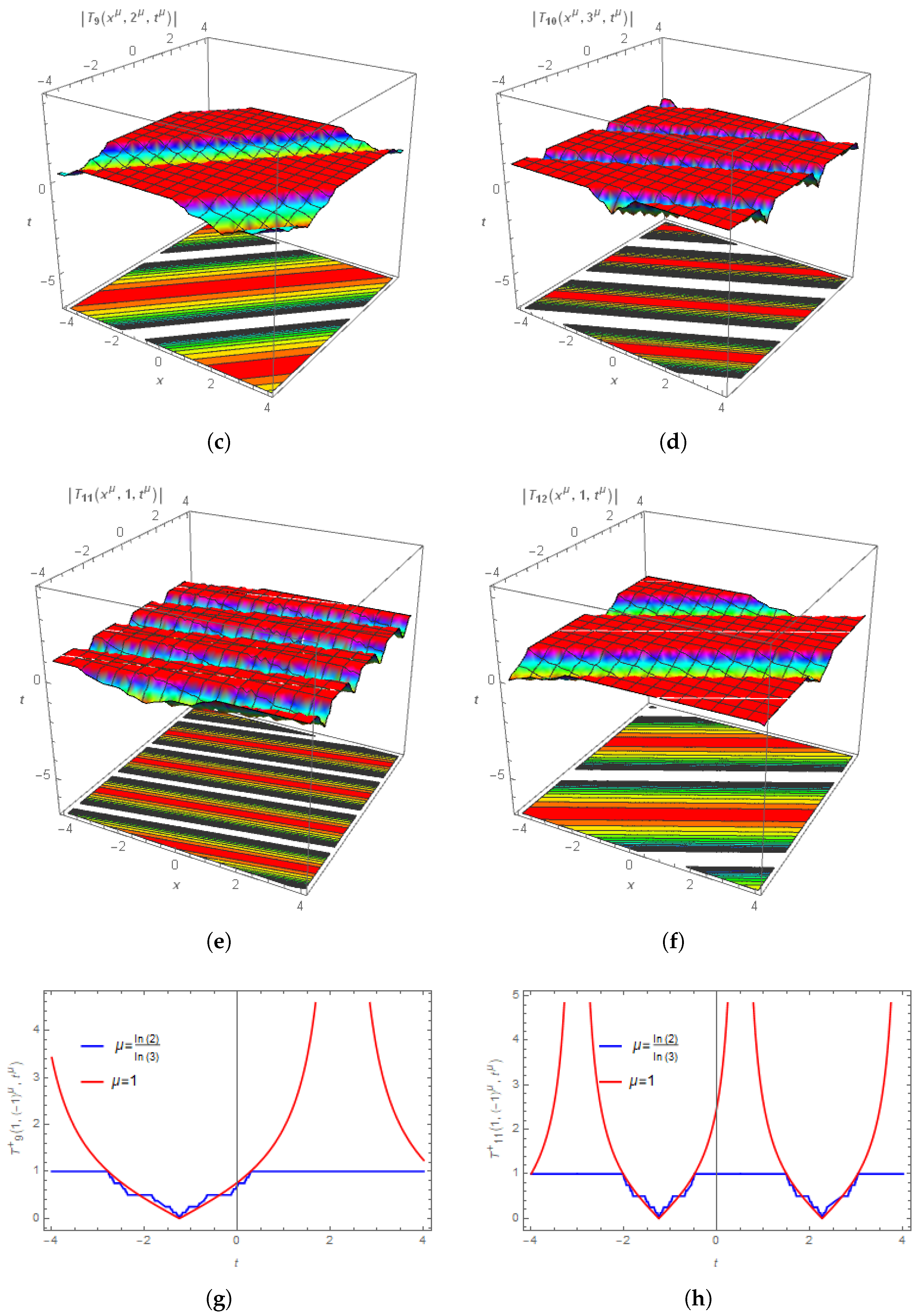
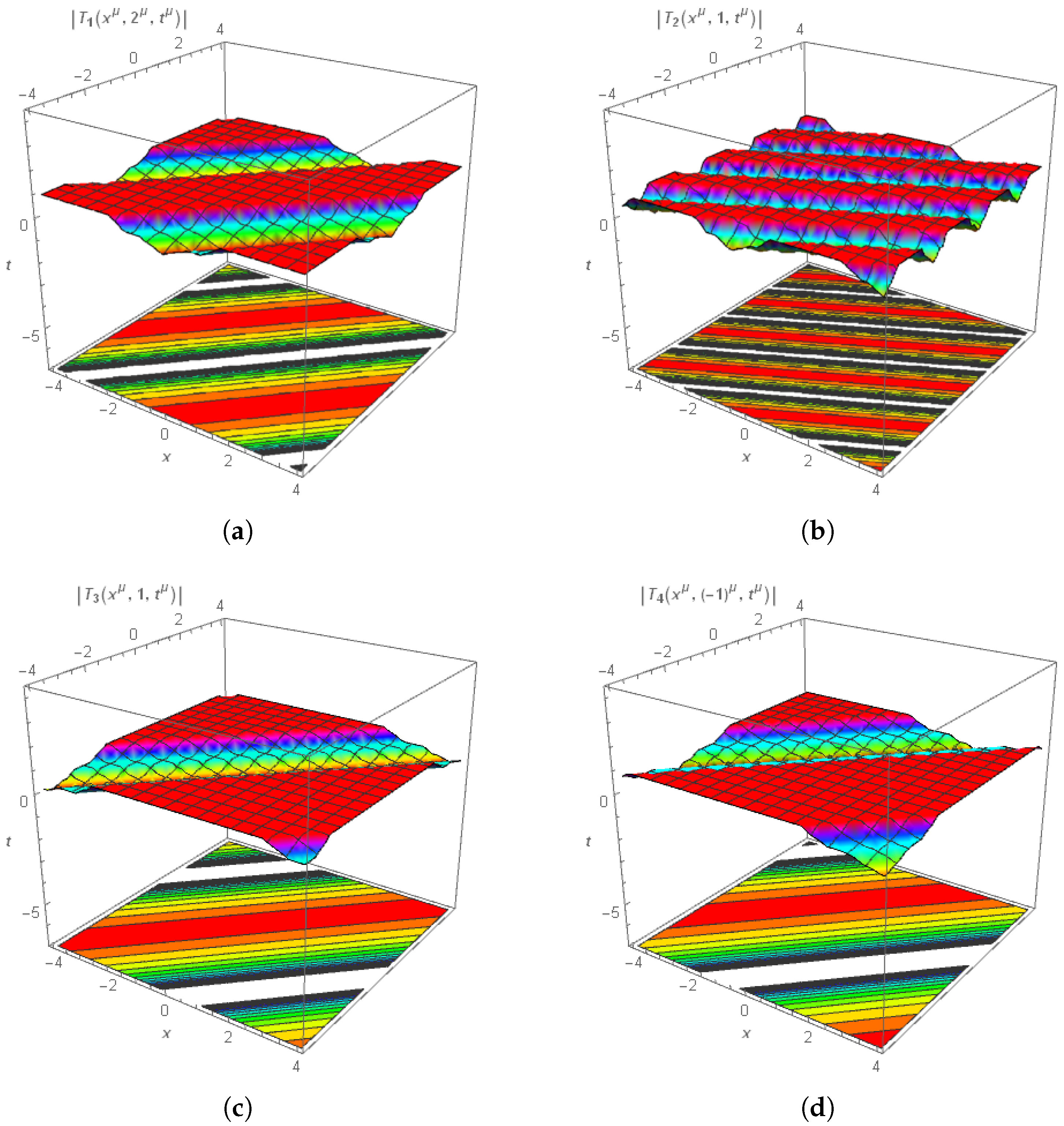
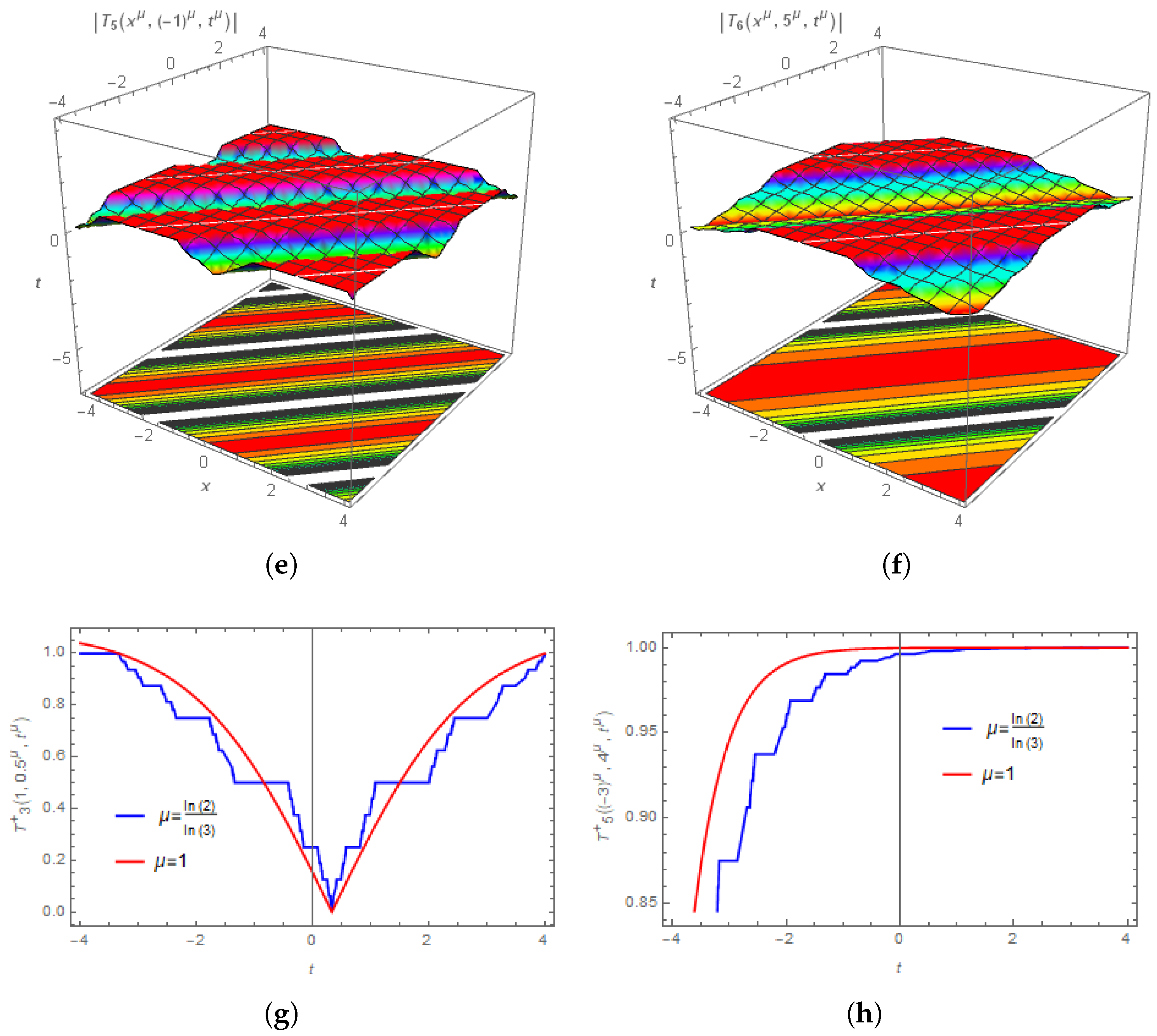
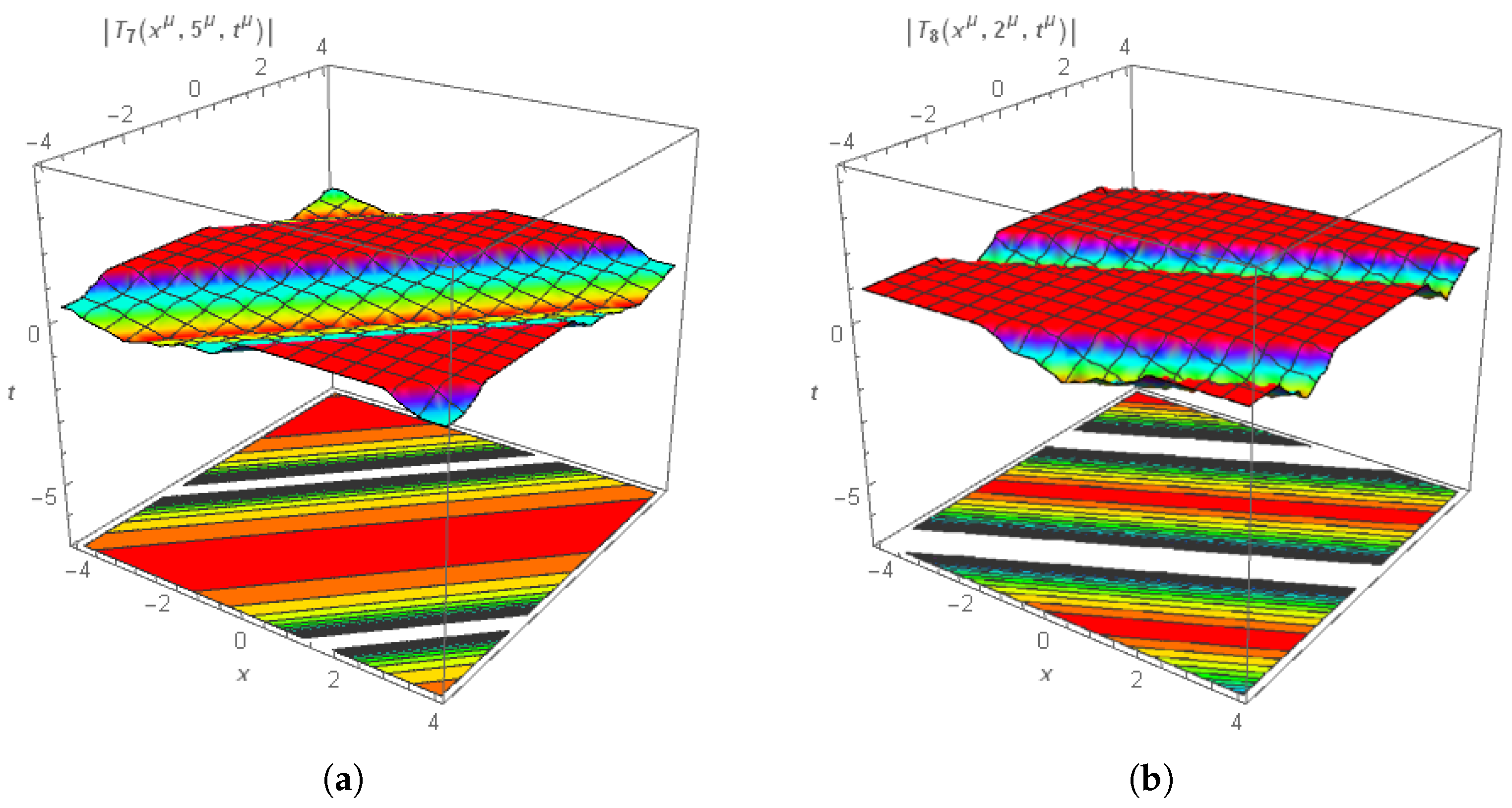
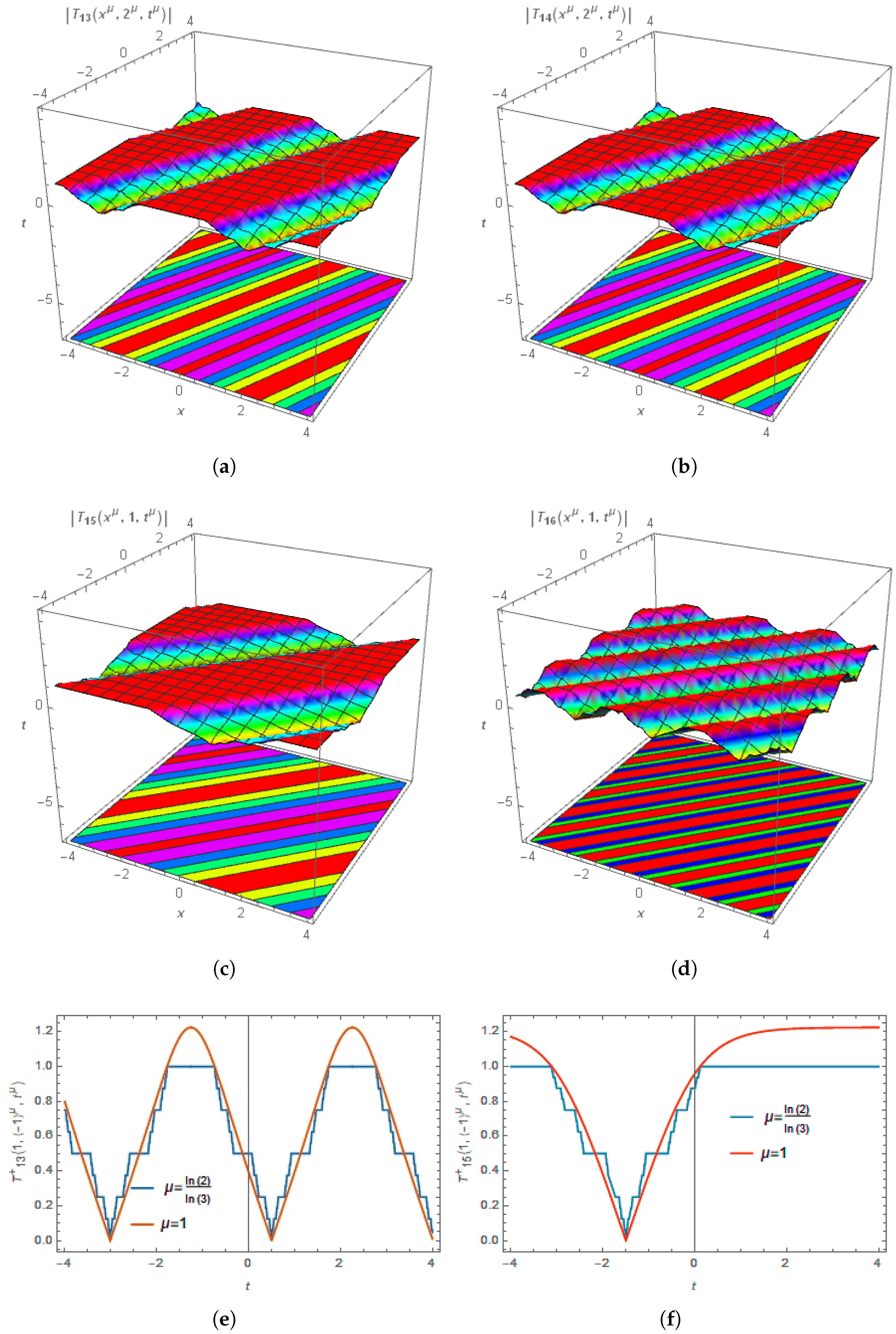
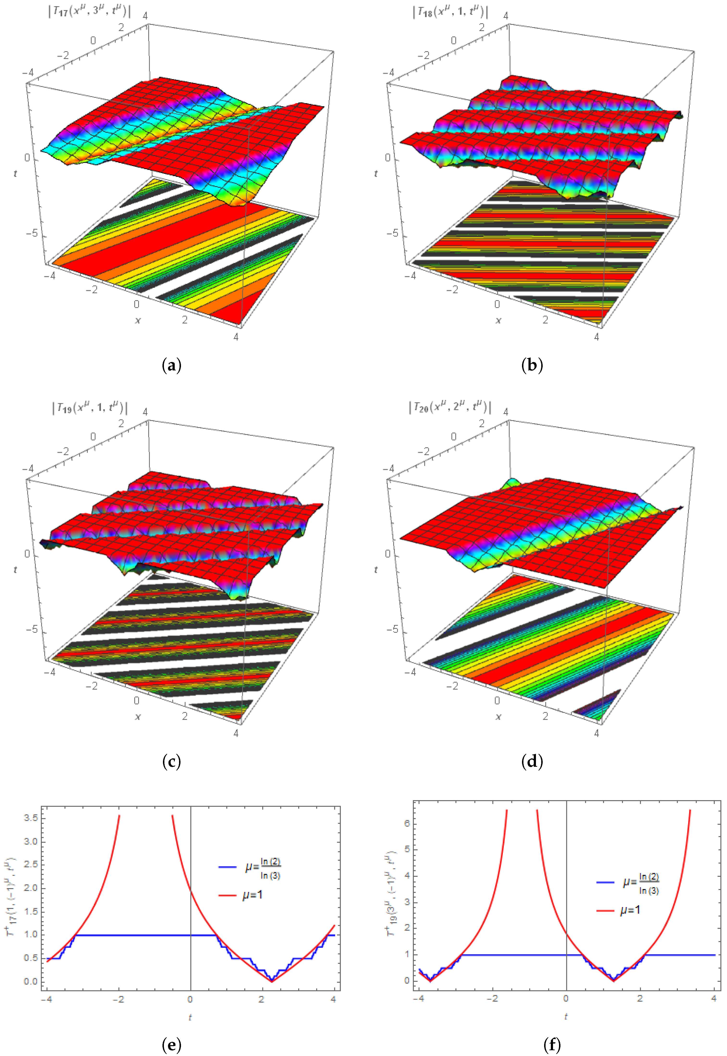
The non-differentiable graphical solution profile of Equation (3) on Cantor sets employing numerous parameters mentioned in the text is discussed in this section. The algebraic mathematical software Mathematica 12.0 is used to simulate each of the graphical solutions. With the aid of several model parameters, we were able to find trigonometric function solutions in Figure 1a through Figure 1f, involving ($|{\mathcal{T}}_1\left(x^{\mu },y^{\mu },t^{\mu }\right)|$ to $|{\mathcal{T}}_6\left(x^{\mu },y^{\mu },t^{\mu }\right)|$). The optical soliton solution behavior of Equation (3) on Cantor sets is exactly described for $\mu ={\displaystyle \frac{In\left(2\right)}{In\left(3\right)}}$. The graphics clearly show the non-differentiable wave behavior across the Cantor sets. We used several parameters in the model ($|{\mathcal{T}}_7\left(x^{\mu },y^{\mu },t^{\mu }\right)|$ to $|{\mathcal{T}}_{12}\left(x^{\mu },y^{\mu },t^{\mu }\right)|$) and were able to discover trigonometric function solutions in Figure 2a–f. The optical soliton solution of Equation (3) on Cantor sets is exactly described for $\mu ={\displaystyle \frac{In\left(2\right)}{In\left(3\right)}}$. The figures show graphically the non-differentiable wave behavior on Cantor sets. In Figure 3a to Figure 3d, we found hyperbolic function solutions (i.e., $|{\mathcal{T}}_{13}\left(x^{\mu },y^{\mu },t^{\mu }\right)|$ to $|{\mathcal{T}}_{16}\left(x^{\mu },y^{\mu },t^{\mu }\right)|$) by using several model parameters. The optical soliton solution behavior of Equation (3) on Cantor sets is exactly described for $\mu ={\displaystyle \frac{In\left(2\right)}{In\left(3\right)}}$. The illustrations vividly depict the non-differentiable wave behavior on the cantor sets. Figure 4a to Figure 4d, we were able to get hyperbolic function solutions by using several model parameters, namely ($|{\mathcal{T}}_{17}\left(x^{\mu },y^{\mu },t^{\mu }\right)|$ to $|{\mathcal{T}}_{20}\left(x^{\mu },y^{\mu },t^{\mu }\right)|$). For $\mu ={\displaystyle \frac{In\left(2\right)}{In\left(3\right)}}$, the optical soliton solution behavior of Equation (3) is shown exactly on Cantor sets. The illustrations clearly show the non-differentiable wave behavior on the Cantor sets. The complex solutions in $|{\mathcal{T}}_{13}\left(x^{\mu },y^{\mu },t^{\mu }\right)|$ to $|{\mathcal{T}}_{16}\left(x^{\mu },y^{\mu },t^{\mu }\right)|$ and $|{\mathcal{T}}_{17}\left(x^{\mu },y^{\mu },t^{\mu }\right)|$ to $|{\mathcal{T}}_{20}\left(x^{\mu },y^{\mu },t^{\mu }\right)|$ are containing both the phase and amplitude of nonlinear waves and at the same time include nonlocal effects, memory and heredity. These properties are crucial tools in modeling wave propagation in quantum systems, optical fibers, plasma physics, and telecommunication systems. The real-valued function solutions reported in $|{\mathcal{T}}_1\left(x^{\mu },y^{\mu },t^{\mu }\right)|$ to $|{\mathcal{T}}_6\left(x^{\mu },y^{\mu },t^{\mu }\right)|$ and $|{\mathcal{T}}_7\left(x^{\mu },y^{\mu },t^{\mu }\right)|$ to $|{\mathcal{T}}_{12}\left(x^{\mu },y^{\mu },t^{\mu }\right)|$ exhibit both the phase and amplitude of nonlinear waves while simultaneously incorporating nonlocal effects, memory, and heredity and preserving the properties of wave propagation with many real-life applications.

7. Modulation Instability Analysis (MI)

In Section 5, the rational sine–cosine scheme is utilized to obtain optical solitons to Equation (3) on Cantor sets, and the non-differentiable graphical solution behavior is presented. The modulation instability analysis is discussed in this section. Setting $\mu =1$ in Equation (3) and using the linear stability method, we assume that Equation (3) has the perturbed steady-state solution in the form

$$\mathcal{U}\left(x,y,t\right)=\mathcal{K}+\Theta \mathcal{N}\left(x,y,t\right),$$

(52)

where $\Theta$ represents the normalized optical power. Using linear stability analysis, we study the evolution of the perturbation in Equation (3). Putting Equation (52) into Equation (3) gives

$$\Theta {\mathcal{N}}_t+{\mathcal{K}}^2\Theta {\lambda }_1{\mathcal{N}}_x+2\mathcal{K}{\Theta }^2{\lambda }_1\mathcal{N}{\mathcal{N}}_x+{\Theta }^3{\lambda }_1{\mathcal{N}}^2{\mathcal{N}}_x+\Theta {\lambda }_2{\mathcal{N}}_{xxx}+\Theta {\lambda }_2{\mathcal{N}}_{yyx}=0.$$

(53)

Linearizing in $\Theta$, we get

$${\mathcal{N}}_t+{\mathcal{K}}^2{\lambda }_1{\mathcal{N}}_x+{\lambda }_2{\mathcal{N}}_{xxx}+{\lambda }_2{\mathcal{N}}_{yyx}=0.$$

(54)

Assume the solution of Equation (54) is

$$\mathcal{N}(x,y,t)=\mathcal{L}\exp \left(i\left(\mathcal{J}x+\mathcal{R}y-\mathcal{P}t\right)\right),$$

(55)

where $\mathcal{L}$ is constant, $\mathcal{J},\mathcal{R}$, and $\mathcal{P}$ are the normalized wave numbers, and $\mathcal{P}$ represents the frequency of the perturbation, respectively. Substituting Equation (55) into Equation (54), we get

$$\begin{array}{c}\hfill -\mathcal{L}\mathcal{P}+\mathcal{J}{\mathcal{K}}^2\mathcal{L}{\lambda }_1-{\mathcal{J}}^3\mathcal{L}{\lambda }_2-\mathcal{J}\mathcal{L}{\mathcal{R}}^2{\lambda }_2=0.\end{array}$$

(56)

Solving for $\mathcal{R}$, we get the dispersion relation as

$$\mathcal{R}=\pm {\displaystyle \frac{1}{\sqrt{\mathcal{J}}\sqrt{{\lambda }_2}}}\sqrt{-\mathcal{P}+\mathcal{J}{\mathcal{K}}^2{\lambda }_1-{\mathcal{J}}^3{\lambda }_2}.$$

(57)

The last equation gives the stability of the steady state. When $\mathcal{R}$ is real, Equation (55) is stable for small disturbances, but when $\mathcal{R}$ is imaginary, Equation (55) is unstable and vice versa, as the related disturbances rise exponentially. Moreover, from Equation (55), the required conditions for the occurrence of modulation instability are

$$\begin{array}{ccc}& & -\mathcal{P}+\mathcal{J}{\mathcal{K}}^2{\lambda }_1-{\mathcal{J}}^3{\lambda }_2<0,\hfill \end{array}$$

(58)

or

$$\begin{array}{ccc}& & \mathcal{J}<0,{\lambda }_2<0.\hfill \end{array}$$

(59)

Thus, the gain spectrum $G\left(\mathcal{P}\right)$ for the modulation instability (IM) is determined by the following equation:

$$G\left(\mathcal{P}\right)=2Im\left(\mathcal{R}\right)=2Im\left({\displaystyle \frac{1}{\sqrt{\mathcal{J}}\sqrt{{\lambda }_2}}}\sqrt{-\mathcal{P}+\mathcal{J}{\mathcal{K}}^2{\lambda }_1-{\mathcal{J}}^3{\lambda }_2}\right).$$

(60)

8. Conclusions

In this paper, we study fmZKe on Cantor sets by employing the extended rational sine–cosine method. We recover a variety of new exact solutions in terms of trigonometric and hyperbolic function solutions. With the help of a computer symbolic system and several parameters mentioned in the text, we plot the three-dimensional and two-dimensional graphical solution profiles of the model and highlight their real-life applications. Additionally, the modulation instability of the model in the classical sense is reported. The solutions achieved by the extended rational sine–cosine method are straightforward, robust, and unique. Furthermore, the suggested fmZKe has many applications in applied physical science and engineering. The model is crucial and, in the future, will be useful for understanding the fractal dynamics of nonlinear phenomena.

References

1. Zakharov, V.E.; Kuznetsov, E.A. Three-dimensional solitons. Zh. Eksp. Teor. Fiz. 1974, 29, 594–597. [Google Scholar]
2. Munro, S.; Parkes, E.J. The derivation of a modified Zakharov-Kuznetsov equation and the stability of its solutions. J. Plasma Phys. 2000, 62, 305–317. [Google Scholar] [CrossRef] [Scilit]
3. Munro, S.; Parkes, E.J. Stability of solitary-wave solutions to a modified Zakharov-Kuznetsov equation. J. Plasma Phys. 2000, 64, 411–426. [Google Scholar] [CrossRef] [Scilit]
4. Li, B.; Yong, C.; Zhang, H. Exact travelling wave solutions for a generalized Zakharov-Kuznetsov equation. Appl. Math. Comput. 2003, 146, 653–666. [Google Scholar] [CrossRef] [Scilit]
5. Shivamoggi, B.K. The Painlev analysis of the Zakharov-Kuznetsov equation. Phys. Scr. 1990, 42, 641. [Google Scholar] [CrossRef] [Scilit]
6. Du, X.X.; Tian, B.; Qu, Q.X.; Yuan, Y.Q.; Zhao, X.H. Lie group analysis, solitons, self-adjointness and conservation laws of the modified Zakharov-Kuznetsov equation in an electron-positron-ion magnetoplasma. Chaos Solitons Local Fract. 2020, 134, 109709. [Google Scholar] [CrossRef] [Scilit]
7. Schamel, H. A modified Korteweg-de Vries equation for ion acoustic waves due to resonant electrons. J. Plasma Phys. 1973, 9, 377–387. [Google Scholar] [CrossRef] [Scilit]
8. Jhangeer, A.; Munawar, M.; Riaz, M.B.; Baleanu, D. Construction of traveling waves patterns of (n + 1)-dimensional modified Zakharov-Kuznetsov equation in plasma physics. Results Phys. 2020, 19, 103330. [Google Scholar] [CrossRef] [Scilit]
9. Zhao, X.; Zhou, H.; Tang, Y.; Jia, H. Travelling wave solutions for modified Zakharov-Kuznetsov equation. Appl. Math. Comput. 2006, 181, 634–648. [Google Scholar] [CrossRef] [Scilit]
10. Al-Ghafri, K.S.; Hadi, R. Solitons and other solutions of (3 + 1)-dimensional space–time fractional modified KdV–Zakharov–Kuznetsov equation. Appl. Math. Nonlinear Sci. 2019, 4, 289–304. [Google Scholar] [CrossRef] [Scilit]
11. Wang, K.J.; Shi, F. A novel computational approach to the local fractional (3 + 1)-dimensional modified Zakharov-Kuznetsov equation. Local Fract. 2024, 32, 2450026. [Google Scholar] [CrossRef] [Scilit]
12. Wang, K.J.; Li, S. Study on the local fractional (3+1)-dimensional modified Zakharov-Kuznetsov equation by a simple approach. Local Fract. 2024, 32, 2450091. [Google Scholar] [CrossRef] [Scilit]
13. Ali, M.N.; Osma, M.S.; Husnine, S.M. On the analytical solutions of conformable time-fractional extended Zakharov-Kuznetsov equation through ( G G )-expansion method and the modified Kudryashov method. SeMA 2019, 76, 15–255. [Google Scholar] [CrossRef] [Scilit]
14. Jhangeer, A.; Hussain, A.; Tahir, S.; Sharif, S. Solitonic, super nonlinear, periodic, quasiperiodic, chaotic waves and conservation laws of modified Zakharov-Kuznetsov equation in transmission line. Commun. Nonlinear Sci. Numer. Simul. 2020, 86, 105254. [Google Scholar] [CrossRef] [Scilit]
15. Herr, S.; Kinoshita, S. The Zakharov–Kuznetsov equation in high dimensions: Small initial data of critical regularity. J. Evol. Equ. 2021, 21, 2105–2121. [Google Scholar] [CrossRef] [Scilit]
16. Seadawy, A.R. Stability analysis for Zakharov-Kuznetsov equation of weakly nonlinear ion-acoustic waves in a plasm. Comput. Math. Appl. 2014, 67, 172–180. [Google Scholar] [CrossRef] [Scilit]
17. Li, Y.; Kai, Y. Chaotic Behavior of the Zakharov-Kuznetsov Equation with Dual-Power Law and Triple-Power Law Nonlinearity Nonlinearity. AppliedMath 2023, 3, 1–9. [Google Scholar] [CrossRef] [Scilit]
18. Deng, C. New exact solutions to the Zakharov–Kuznetsov equation and its generalized form. Commun. Nonlinear Sci. Numer. Simul. 2010, 15, 857–868. [Google Scholar] [CrossRef] [Scilit]
19. Wazwaz, A.M. Exact solutions with solitons and periodic structures for the Zakharov-Kuznetsov (ZK) equation and its modified form. Commun. Nonlinear Sci. Numer. Simul. 2005, 10, 597–606. [Google Scholar] [CrossRef] [Scilit]
20. Biswas, A.; Zerrad, E. 1-soliton solution of the Zakharov-Kuznetsov equation with dual-power law nonlinearity. Commun. Nonlinear Sci. Numer. Simul. 2009, 14, 3574–3577. [Google Scholar] [CrossRef] [Scilit]
21. Mohammed, W.W.; Sidaoui, R.; Alshammari, H.W.; Algolam, M.S. Random wave equation for the Stochastic Quantum Zakharov-Kuznetsov equation and their exact solutions. Eur. J. Pure Appl. Math. 2025, 18, 5665. [Google Scholar] [CrossRef] [Scilit]
22. Nirmala, A.N.; Kumbinarasaiah, S. An intriguing numerical strategy for Zakharov–Kuznetsov equation through graph-theoretic polynomials. Phys. Scr. 2024, 99, 095267. [Google Scholar] [CrossRef] [Scilit]
23. Mushtaq, A.; Shah, H.A. Nonlinear Zakharov–Kuznetsov equation for obliquely propagating two-dimensional ion-acoustic solitary waves in a relativistic, rotating magnetized electron-positron-ion plasma. Phys. Plasmas 2005, 12, 072306. [Google Scholar] [CrossRef] [Scilit]
24. Ma, Y.; Wang, Z. Bifurcation and exact solutions of space-time fractional simplified modified Camassa-Holm equation. Fractals 2023, 31, 2350085. [Google Scholar] [CrossRef] [Scilit]
25. Zheng, Z.; Menf, H.; Zhang, J.; Wang, Z. Bifurcations and traveling wave solutions of the space-time fractional coupled Boussinesq equations. Fractals 2025, 33, 2550065. [Google Scholar] [CrossRef] [Scilit]
26. Xu, H.; Liu, M.; Wang, Z. Bifurcation and exact traveling wave solutions of fractional Date–Jimbo–Kashiwara–Miwa equation. Fractals 2024, 32, 2450116. [Google Scholar] [CrossRef] [Scilit]
27. Liu, M.; Xu, H.; Wang, Z.; Chen, G. Exact solutions and bifurcation of a modified generalized multidimensional fractional Kadomtsev–Petviashvili equatio. Fractals 2024, 32, 2450046. [Google Scholar] [CrossRef] [Scilit]
28. Saha Ray, S.; Sahoo, S. New Exact Solutions of Fractional Zakharov–Kuznetsov and Modified Zakharov–Kuznetsov Equations Using Fractional Sub-Equation Method. Commun. Theor. Phys. 2015, 63, 25–30. [Google Scholar] [CrossRef] [Scilit]
29. Eslami, M.; Vajargah, B.F.; Mirzazadeh, M. Exact solutions of modified Zakharov–Kuznetsov equation by the homogeneous balance method. Ain Shams Eng. J. 2014, 5, 221–225. [Google Scholar] [CrossRef] [Scilit]
30. Tascan, F.; Bekir, A. Travelling wave solutions of nonlinear evolution equations by using the first integral method. Commun. Nonlinear Sci. Numer. Simul. 2009, 14, 1810–1815. [Google Scholar] [CrossRef] [Scilit]
31. Yang, X.J.; Srivastava, H.M.; Baleanu, D. Local Fractional Integral Transform and Their Applications; Academics Press: Cambridge, MA, USA, 2015. [Google Scholar]
32. Yang, X.J.; Machado, J.A.T.; Baleanu, D. Exact traveling wave solutions to the local fractional Boussinesq equation in local fractional domain. Local Fract. 2017, 25, 170006. [Google Scholar] [CrossRef] [Scilit]
33. Bolotov, V.N.; Yu, V. Tkach local fractional Communication System. Tech. Phys. 2008, 53, 1192–1196. [Google Scholar]
34. Malyshev, G.S.; Raevskii, A.S. On the Transmission of a local fractional Pulse in a Noisy Fiber Optic Channel. Tech. Phys. Lett. 2013, 39, 787–790. [Google Scholar] [CrossRef] [Scilit]
35. Goufo, E.F.D. On the local fractional dynamics for higher order traveling waves. Chaos Solitons Local Fract. 2021, 148, 111059. [Google Scholar] [CrossRef] [Scilit]
36. Yang, X.J.; Gasimov, Y.S.; Gao, F.; Allahverdiyeva, N. Travelling-wave solutions for Klein-Gordon and Helmholtz equations on Cantor sets. Proc. Inst. Math. Mech. 2017, 43, 123–131. [Google Scholar]
37. Kang-Jia, W.; Jing, S. On new abundant exact traveling wave solutions to the local fractional Gardner equation defined on Cantor sets. Math. Methods Appl. Sci. 2022, 45, 1904–1915. [Google Scholar] [CrossRef] [Scilit]
38. Ghanbari, B. On the non-differentiable exact solutions to Schamel’s equation with local fractional derivative on Cantor sets. Numer. Methods Partial. Differ. Equ. 2022, 38, 1255–1270. [Google Scholar] [CrossRef] [Scilit]
39. Kang-Jia, W.; Jing, S. On the non-differentiable exact solutions of the (2 + 1)-dimensional local fractional breaking soliton equation on Cantor sets. Math. Methods Appl. Sci. 2023, 46, 1456–1465. [Google Scholar] [CrossRef] [Scilit]
40. Maitama, S.; Zhao, W. Local fractional homotopy analysis method for solving non-differentiable problems on Cantor sets. Adv. Differ. Equ. 2019, 2019, 127. [Google Scholar] [CrossRef] [Scilit]
41. Parvate, A.; Gangal, A.D. Calculus on local fractional subsets of real line-I: Formulation. Local Fract. 2009, 17, 53–81. [Google Scholar]
42. Parvate, A.; Gangal, A.D. Calculus on local fractional subsets of real line-II: Conjugacy with ordinary calculus. Local Fract. 2011, 19, 271–290. [Google Scholar]
43. Satin, S.E.; Parvate, A.; Gangal, A. Fokker-Planck equation on local fractional curves. Chaos Solitons Fractals 2013, 52, 30–35. [Google Scholar]
44. Mandelbrot, B.B. The Fractal Geometry of Nature; W. H. Freeman: New York, NY, USA, 1982. [Google Scholar]
Figure 1. | T 1 + x μ , y μ , t μ | to | T 4 + x μ , y μ , t μ | are singular soliton solutions, while | T 5 + x μ , y μ , t μ | and | T 4 + x μ , y μ , t μ | are periodic soliton solutions of Equation (3) on the Cantor sets using different parameters 4 x 4 and different time intervals. Top: 3D surface solution; bottom: contour surface solution. (a) | T 1 + x μ , y μ , t μ | : ζ 1 μ = 3 , ζ 2 μ = 1 , ζ 3 μ = 3 , y μ = 2 , λ 1 = 3 , and λ 2 = 2 ; (b) | T 2 + x μ , y μ , t μ | : Contour ζ 1 μ = 1 , ζ 2 μ = 1 , ζ 3 μ = 2 , y μ = 1 , λ 1 = 6 , and λ 2 = 1 ; (c) | T 3 + x μ , y μ , t μ | : ζ 1 μ = 3 , ζ 2 μ = 1 , ζ 3 μ = 3 , y μ = 1 , λ 1 = 2 , and λ 2 = 4 ; (d) | T 4 + x μ , y μ , t μ | : Contour ζ 1 μ = 0.5 , ζ 2 μ = 1 , ζ 3 μ = 0.5 , y μ = 1 , λ 1 = 2 , and λ 2 = 1 ; (e) | T 5 + x μ , y μ , t μ | : ζ 1 μ = 5 , ζ 2 μ = 1 , ζ 3 μ = 5 , y μ = 1 , λ 1 = 2 , and λ 2 = 1 ; (f) | T 6 + x μ , y μ , t μ | : Contour ζ 1 μ = 2 , ζ 2 μ = 3 , ζ 3 μ = 2 , y μ = 5 , λ 1 = 7 , and λ 2 = 1 ; (g) | T 3 + x μ , y μ , t μ | : ζ 1 μ = 3 , ζ 2 μ = 1 , ζ 3 μ = 3 , y μ = 2 , λ 1 = 3 , x μ = 1 , and λ 2 = 2 ; (h) | T 5 + x μ , y μ , t μ | : ζ 1 μ = 2 , ζ 2 μ = 1 , ζ 3 μ = 2 , y μ = 4 , λ 1 = 3 , x μ = 3 , and λ 2 = 2 .
Fractalfract 10 00574 g001aFractalfract 10 00574 g001b
Figure 2. | T 7 + x μ , y μ , t μ | to | T 10 + x μ , y μ , t μ | are singular soliton solutions, while | T 11 + x μ , y μ , t μ | and | T 12 + x μ , y μ , t μ | are periodic soliton solutions of Equation (3) on the Cantor sets by using different parameters on 4 x 4 and different time intervals. Top: 3D surface solution; bottom: contour surface solution. (a) | T 7 + x μ , y μ , t μ | : ζ 1 μ = 2 , ζ 2 μ = 3 , ζ 3 μ = 2 , y μ = 5 , λ 1 = 7 , and λ 2 = 1; (b) | T 8 + x μ , y μ , t μ | : Contour ζ 1 μ = 1 , ζ 2 μ = 3 , ζ 3 μ = 2 , y μ = 2 , λ 1 = 2 , and λ 2 = 1 ; (c) | T 9 + x μ , y μ , t μ | : ζ 1 μ = 2 , ζ 2 μ = 1 , ζ 3 μ = 2 , y μ = 2 , λ 1 = 2 , and λ 2 = 2 ; (d) | T 10 + x μ , y μ , t μ | : Contour ζ 1 μ = 1 , ζ 2 μ = 1 , ζ 3 μ = 2 , y μ = 3 , λ 1 = 1 , and λ 2 = 2 ; (e) | T 11 + x μ , y μ , t μ | : ζ 1 μ = 1 , ζ 2 μ = 1 , ζ 3 μ = 2 , y μ = 1 , λ 1 = 3 , and λ 2 = 2 ; (f) | T 12 + x μ , y μ , t μ | : Contour ζ 1 μ = 2 , ζ 2 μ = 3 , ζ 3 μ = 2 , y μ = 5 , λ 1 = 7 , and λ 2 = 1 ; (g) | T 9 + x μ , y μ , t μ | : ζ 1 μ = 2 , ζ 2 μ = 1 , ζ 3 μ = 2 , y μ = 1 , λ 1 = 2 , x μ = 1 , and λ 2 = 2 ; (h) | T 11 + x μ , y μ , t μ | : ζ 1 μ = 2 , ζ 2 μ = 1 , ζ 3 μ = 2 , y μ = 1 , λ 1 = 2 , x μ = 1 , and λ 2 = 2 .
Fractalfract 10 00574 g002aFractalfract 10 00574 g002b
Figure 3. | T 13 + x μ , y μ , t μ | and | T 14 + x μ , y μ , t μ | are dark soliton solutions, while | T 11 + x μ , y μ , t μ | and | T 12 + x μ , y μ , t μ | are periodic soliton solutions of Equation (3) on the Cantor sets by using different parameters 4 x 4 and different time intervals. Top: 3D surface solution; bottom: contour surface solution. (a) | T 13 + x μ , y μ , t μ | : ζ 1 μ = 2 , ζ 2 μ = 0.5 , ζ 3 μ = 1 , y μ = 2 , λ 1 = 0.5 , and λ 2 = 2 ; (b) | T 14 + x μ , y μ , t μ | : ζ 1 μ = 2 , ζ 2 μ = 0.5 , ζ 3 μ = 1 , y μ = 2 , λ 1 = 0.5 , and λ 2 = 2 ; (c) | T 15 + x μ , y μ , t μ | : ζ 1 μ = 1 , ζ 2 μ = 2 , ζ 3 μ = 1 , y μ = 1 , λ 1 = 1 , and λ 2 = 2 ; (d) | T 16 + x μ , y μ , t μ | : ζ 1 μ = 4 , ζ 2 μ = −2, ζ 3 μ = 4 , y μ = 1 , λ 1 = 2 , and λ 2 = 1 ; (e) | T 13 + x μ , y μ , t μ | : ζ 1 μ = 2 , ζ 2 μ = 1 , ζ 3 μ = 2 , y μ = 1 , λ 1 = −2, x μ = 1 , and λ 2 = 2 ; (f) | T 15 + x μ , y μ , t μ | : ζ 1 μ = 2 , ζ 2 μ = 1 , ζ 3 μ = 2 , y μ = 1 , λ 1 = 2 , x μ = 1 , and λ 2 = 2 .
Fractalfract 10 00574 g003
Figure 4. | T 17 + x μ , y μ , t μ | and | T 18 + x μ , y μ , t μ | are singular soliton solutions, while | T 11 + x μ , y μ , t μ | and | T 12 + x μ , y μ , t μ | are periodic soliton solutions of Equation (3) on the Cantor sets by using different parameters 4 x 4 and different time intervals. Top: 3D surface solution; bottom: contour surface solution. (a) | T 17 + x μ , y μ , t μ | : ζ 1 μ = 4 , ζ 2 μ = 1 , ζ 3 μ = 2 , y μ = 3 , λ 1 = 2 , and λ 2 = 1 ; (b) | T 18 + x μ , y μ , t μ | : ζ 1 μ = 1 , ζ 2 μ = 2 , ζ 3 μ = 2 , y μ = 1 , λ 1 = 4 , and λ 2 = 0.5 ; (c) | T 19 + x μ , y μ , t μ | : ζ 1 μ = 2 , ζ 2 μ = 1 , ζ 3 μ = 3 , y μ = 1 , λ 1 = 1 , and λ 2 = 1 ; (d) | T 20 + x μ , y μ , t μ | : ζ 1 μ = 2 , ζ 2 μ = −0.5, ζ 3 μ = 1, y μ = 2 , λ 1 = 0.5 , and λ 2 = 1 ; (e) | T 17 + x μ , y μ , t μ | : ζ 1 μ = 2 , ζ 2 μ = 1 , ζ 3 μ = 2 , y μ = 1 , λ 1 = −2, x μ = 1 , and λ 2 = 2 ; (f) | T 19 + x μ , y μ , t μ | : ζ 1 μ = 1 , ζ 2 μ = 2 , ζ 3 μ = 2 , y μ = 1 , λ 1 = 2 , x μ = 3 , and λ 2 = 1 .
Fractalfract 10 00574 g004
Disclaimer/Publisher’s Note: The statements, opinions and data contained in all publications are solely those of the individual author(s) and contributor(s) and not of MDPI and/or the editor(s). MDPI and/or the editor(s) disclaim responsibility for any injury to people or property resulting from any ideas, methods, instructions or products referred to in the content.