Analytical and Numerical Solution Methods for Some Space-Fractional Reaction–Diffusion Systems via Hankel Transforms

Abstract

Diffusion within porous media, such as biological tissues, often deviates from conventional Fick’s laws that may be described by space-fractional diffusion equations. Microscale tissue heterogeneity can be represented by the space-fractional Riesz Laplacian operator acting on concentration or, alternatively, by fractional a Riesz gradient of the order $\beta$, extending the usual spatial gradient concept. We consider a reaction-diffusion system with two spatial compartments—a proximal one of finite radius having a source, and an outer one extending to infinity where the source is absent but first-order decay takes place. The steady state is derived using Hankel and Mellin transforms, resulting in integral-kernels-containing Bessel functions. We develop and compare three numerical quadrature methods for the Hankel transform: sinc quadrature, Ogata quadrature (based on Bessel zeros), and a hybrid asymptotic–numerical scheme. Numerical results and plots are presented for exponents $\beta =1/2,2/3,3/4$ and 1. The integer-order case ($\beta =1$) is recovered as a limiting case. The hybrid method is about five times faster than the global quadratures for the same accuracy. The novelty of this work lies in the systematic comparison of numerical methods for this specific class of fractional reaction–diffusion problems.

1. Introduction

Over the past few decades, fractional diffusion equations have become important for modeling anomalous transport in biological tissues, turbulent flows, and disordered media [1,2,3,4]. The Riesz fractional Laplacian, in particular, is widely used to model space-fractional diffusion [5,6].

Many physical problems involving cylindrical, axial, or radial symmetry admit solutions represented by integrals containing Bessel functions of the first kind. Such representations arise naturally through the Hankel transform [7], which takes the form

$${\mathcal{H}}_{\nu }\left[f\right]\left(s\right)={\int }_0^{\infty }f\left(x\right)J_{\nu }\left(sx\right)xdx,$$

(1)

where $J_{\nu }$ denotes the Bessel function of the first kind of order $\nu$. Applications include transport around fibers, electrodes, blood vessels, cylindrical inclusions, and localized sources in effectively two-dimensional media. Under these symmetries, the multidimensional Fourier transform reduces naturally to a Hankel transform. The order $\nu$ is determined by the spatial dimension and symmetry class; in particular, $\nu =0$ applies to radially symmetric fields in two dimensions.

Consequently, reliable numerical evaluation of oscillatory Hankel-type integrals becomes a central computational task. This evaluation is especially challenging when the integrand exhibits algebraic singularities, slowly decaying tails, rapidly oscillating Bessel kernels, or fractional powers of the transform variable. Such features commonly occur in Green-function representations of space-fractional diffusion problems and can render direct quadrature inaccurate or computationally expensive. Efficient numerical methods for Hankel integrals are therefore essential for the analysis and simulation of radially symmetric fractional transport models.

2. Physical Background

Diffusion in porous and structurally heterogeneous media, including biological tissues, may deviate from the classical Fickian description [4,8]. One important class of anomalous transport processes is space-fractional diffusion, which may arise as a scaling limit of a continuous-time random walk (CTRW) whose jump lengths belong to the domain of attraction of a symmetric Lévy stable distribution [1]. In an unbounded domain, conservation of mass is expressed by the continuity equation

$${\partial }_{t}c+\nabla ·\mathbf{j}=0,$$

(2)

where $c=c(\mathbf{x},t)$ is the concentration and $\mathbf{j}$ denotes the vector-valued diffusive flux.

We introduce a generalized first Fick law,

$$\mathbf{j}=-D_{\alpha }{\nabla }^{\beta }c,0\le \beta \le 1,$$

(3)

in terms of the Riesz fractional gradient ${\nabla }^{\beta }$ [9]. In Fourier space, this operator is defined by

$$\mathcal{F}\left[{\nabla }^{\beta }c\right]\left(\mathbf{k}\right)={i\mathbf{k}\left|\mathbf{k}\right|}^{\beta -1}\widehat{c}\left(\mathbf{k}\right)=i{\mathbf{k}}^0{\left|\mathbf{k}\right|}^{\beta }\widehat{c}\left(\mathbf{k}\right),{\mathbf{k}}^0:={\displaystyle \frac{\mathbf{k}}{\left|\mathbf{k}\right|}}.$$

(4)

Equivalently,

$${\nabla }^{\beta }=\nabla {(-\mathrm{\Delta })}^{(\beta -1)/2}.$$

(5)

Thus, ${\nabla }^{\beta }$ interpolates between the vector Riesz transform

$${\nabla }^0=\nabla {(-\mathrm{\Delta })}^{-1/2},$$

(6)

at $\beta =0$, and the ordinary gradient,

$${\nabla }^1=\nabla ,$$

(7)

at $\beta =1$. Unlike the scalar Riesz fractional Laplacian and the scalar Riesz potential, the Riesz fractional gradient remains vector valued. Furthermore, the above definition is objective in the sense discussed in [10].

Taking the divergence of (4) gives

$$\mathcal{F}\left[\nabla ·{\nabla }^{\beta }c\right]\left(\mathbf{k}\right)=-{\left|\mathbf{k}\right|}^{1+\beta }\widehat{c}\left(\mathbf{k}\right).$$

(8)

Therefore, combining (2) and (3) yields the non-local, integro-differential system

$${\partial }_{t}c=-D_{\alpha }{(-\mathrm{\Delta })}^{\alpha }c,\alpha ={\displaystyle \frac{1+\beta }{2}},$$

(9)

where the Riesz fractional Laplacian is defined by its Fourier symbol [5]

$$\mathcal{F}\left[{(-\mathrm{\Delta })}^{\alpha }c\right]\left(\mathbf{k}\right)={\left|\mathbf{k}\right|}^{2\alpha }\widehat{c}\left(\mathbf{k}\right).$$

(10)

The classical Fick law is recovered for $\beta =1$, for which $\alpha =1$, ${\nabla }^{\beta }=\nabla$, and $\mathbf{j}=-D_1\nabla c$. For $0\le \beta <1$, the flux–concentration relation is nonlocal.

It is convenient to introduce the spatial stable index

$$\mu :=2\alpha =1+\beta .$$

(11)

Thus, the present formulation covers the range $1\le \mu \le 2$, or, equivalently, $1/2\le \alpha \le 1$. The parameter $\mu$ is the characteristic exponent of the associated symmetric Lévy stable process. The case $\mu =2$ ($\alpha =1$, $\beta =1$) recovers the Gaussian heat equation and the classical Fick law. For $1\le \mu <2$, the model describes space-fractional, or Lévy-flight, superdiffusion characterized by nonlocal transport and heavy-tailed jump distributions.

For an initial point source, the fundamental solution satisfies

$$\widehat{p}(\mathbf{k},t)=exp\left[-D_{\alpha }t{\left|\mathbf{k}\right|}^{\mu }\right].$$

(12)

For $1\le \mu <2$, its far-field behavior is algebraic,

$$p(\mathbf{x},t)\sim C_{\mu ,d}{\left(t\right)\left|\mathbf{x}\right|}^{-d-\mu },\left|\mathbf{x}\right|\to \infty ,$$

(13)

where $C_{\mu ,d}\left(t\right)$ is a time-dependent coefficient. At $\mu =2$, in contrast, the propagator is Gaussian and decays exponentially in ${\left|\mathbf{x}\right|}^2$.

Accordingly, $\beta$ parametrizes the degree of nonlocality in the generalized flux law, whereas $\mu =1+\beta$ determines the stable-law index and the far-field decay exponent. In heterogeneous porous media, $\beta$ may be interpreted phenomenologically as an effective descriptor of unresolved microstructural heterogeneity and long-range transport pathways.

The present work develops and compares three numerical quadrature methods for the Hankel transform: sinc quadrature, Ogata method (based on Bessel J zeros), and a hybrid asymptotic-numerical scheme.

3. The Reaction-Diffusion System

We consider a first-order reaction–diffusion system in two dimensions [11]

$${\partial }_{t}c=-D{(-\mathrm{\Delta })}^{\alpha }c+\sigma -qc,0<\alpha \le 1,$$

(14)

where $\sigma$ is the intensity of the spatially-extended source, and q is an elimination rate. The system can support a non-trivial steady state, which will be studied in the present contribution. The system supports a non-trivial steady state, which is the focus of the present contribution.

We assume cylindrical geometry of infinite extent. The system is compartmentalized into a proximal compartment of radius L (having source intensity $\sigma$) and an outer compartment extending to infinity (no source, only first-order decay). The source term S therefore splits into $S_i=\sigma -qc$ (proximal) and $S_o=-qc$ (distal) parts.

The steady state of the system (Equation (14)) can be written as

$$-D{(-\mathrm{\Delta })}^{\alpha }c\left(r\right)+\sigma -qc\left(r\right)=0,$$

(15)

with boundary condition $c(\infty )=0$ [9]. For full physical fidelity, the equation should be non-dimensionalized. To non-dimensionalize Equation (15), we recall that ${\mathcal{H}}_0\left[{(-\mathrm{\Delta })}^{\alpha }c\right]={\rho }^{2\alpha }\widehat{c}\left(\rho \right)$. We introduce a characteristic length scale $r_0$ and time scale $t_0$ such that the dimensionless spatial variable is $\tilde{r}=r/r_0$. By imposing the condition $D{t}_0/r_0^{2\alpha }=1$, the diffusion coefficient is normalized to unity ($D=1$), and the equation is rendered dimensionless through the re-parametrization of the source and decay terms. Hence, to simplify presentation we set D = 1.

4. Analytical Solutions

4.1. Integer-Order Case $\alpha =\mathsf{1}$

For $\alpha =1$ the Laplacian is local, and the system splits into two disjoint compartments that interact only at their mutual boundary. The full solution is [9]

$$c\left(r\right)=\mathbf{1}(L-r)c_p\left(r\right)+\mathbf{1}(r-L)c_d\left(r\right),$$

where $\mathbf{1}(·)$ denotes the unit step function ($\mathbf{1}\left(0\right)=1/2$). Here, $c_p\left(r\right)$ denotes the concentration in the proximal compartment $0\le r\le L$, while $c_d\left(r\right)$ denotes the concentration in the distal compartment $r\ge L$. The piecewise definition ensures continuity at the interface $r=L$. Using cylindrical coordinates we obtain the modified Bessel equation of order 0 as the homogeneous part of the system:

$${\displaystyle \frac{1}{r}}\left[c_p^{\prime }\left(r\right)+r{c}_p^{″}\left(r\right)\right]-q{c}_p\left(r\right)=-\sigma ,$$

(16)

Using standard decay and boundedness arguments, we obtain the indeterminate solution

$$c_p\left(r\right)={\displaystyle \frac{\sigma }{q}}+k_1{I}_0\left(\sqrt{q}r\right),c_d\left(r\right)=k_2{K}_0\left(\sqrt{q}r\right).$$

(17)

Matching conditions at the $r=L$ boundary, that is $c_p\left(L\right)=c_d\left(L\right)$ and $c_p^{\prime }\left(L\right)=c_d^{\prime }\left(L\right)$, uniquely fixes the coefficients

$$k_1=-{\displaystyle \frac{K_1\left(L\sqrt{q}\right)\sigma }{Pq}},k_2={\displaystyle \frac{I_1\left(L\sqrt{q}\right)\sigma }{Pq}},P={\displaystyle \frac{1}{L\sqrt{q}}},$$

(18)

where the Wronskian identity $K_0\left(x\right)I_1\left(x\right)+I_0\left(x\right)K_1\left(x\right)=1/x$ has been used to simplify the denominator [12]. Hence, the final integer-order solution is

$$c_p\left(r\right)={\displaystyle \frac{\sigma }{q}}-{\displaystyle \frac{\sigma L}{\sqrt{q}}}{K}_1\left(\sqrt{q}L\right)I_0\left(\sqrt{q}r\right),$$

(19)

$$c_d\left(r\right)={\displaystyle \frac{\sigma L}{\sqrt{q}}}{I}_1\left(\sqrt{q}L\right)K_0\left(\sqrt{q}r\right).$$

(20)

Figure 1 compares the inner and outer solutions.

4.2. Fractional-Order Case

For the fractional case the solution can be obtained in the Fourier–Hankel domain in an equivalent way. Using the Hankel transform (Appendix A) and noting that the source term $\sigma \left(r\right)=\sigma \mathbf{1}(L-r)$ has Hankel transform

$${\mathcal{H}}_0\left[\sigma \left(r\right)\right]=\sigma L{J}_1\left(\rho L\right)/\rho$$

we obtain the transformed equation

$$-{\rho }^{2\alpha }\widehat{c}+\sigma L{\displaystyle \frac{J_1\left(\rho L\right)}{\rho }}-q\widehat{c}=0,$$

(21)

in the Fourier–Hankel domain. Hence,

$$\widehat{c}=\sigma L{\displaystyle \frac{J_1\left(\rho L\right)}{\rho ({\rho }^{2\alpha }+q)}}.$$

(22)

Transforming back to the spatial domain gives the integral representation

$$c\left(r\right)=\sigma L{\int }_0^{\infty }{\displaystyle \frac{J_0\left(\rho r\right)J_1\left(\rho L\right)}{{\rho }^{2\alpha }+q}}d\rho ,2\alpha =1+\beta .$$

(23)

Convergence, existence, and regularity of the integral in Equation (23): For $r>0$ and $\alpha >0$, the integrand behaves as $\mathcal{O}\left({\rho }^{-(2\alpha +1)}\right)$ as $\rho \to \infty$ because the Bessel functions are asymptotically $\mathcal{O}\left({\rho }^{-1/2}\right)$. Since $2\alpha +1>1$, the integral converges absolutely. The solution is smooth for $r>0$ and $r\ne L$, with possible logarithmic singularities in derivatives at $r=L$. The decay at infinity is algebraic, $c\left(r\right)=\mathcal{O}\left(r^{-(2\alpha +2)}\right)$, as shown later in Equation (32). It is important to note that the kernel in Equation (23) contains the standard Bessel functions $J_0$ and $J_1$, which arise naturally from the inverse Hankel transform of the radially symmetric problem. This is in contrast to the modified Bessel functions $I_0$ and $K_0$ that appear in the integer-order local case. The standard Bessel functions guarantee the correct oscillatory-to-decaying behavior in the Fourier domain and ensure $c\left(r\right)\to 0$ as $r\to \infty$ for the fractional case.

4.3. Asymptotic Solution on a Ring Source

For a fictitious delta source on the boundary $r=L$ we obtain

$$c_d\left(r\right)={\sigma }^{\prime }{\int }_0^{\infty }{\displaystyle \frac{J_0\left(\rho r\right)J_0\left(\rho L\right)\rho }{{\rho }^2+q}}d\rho .$$

(24)

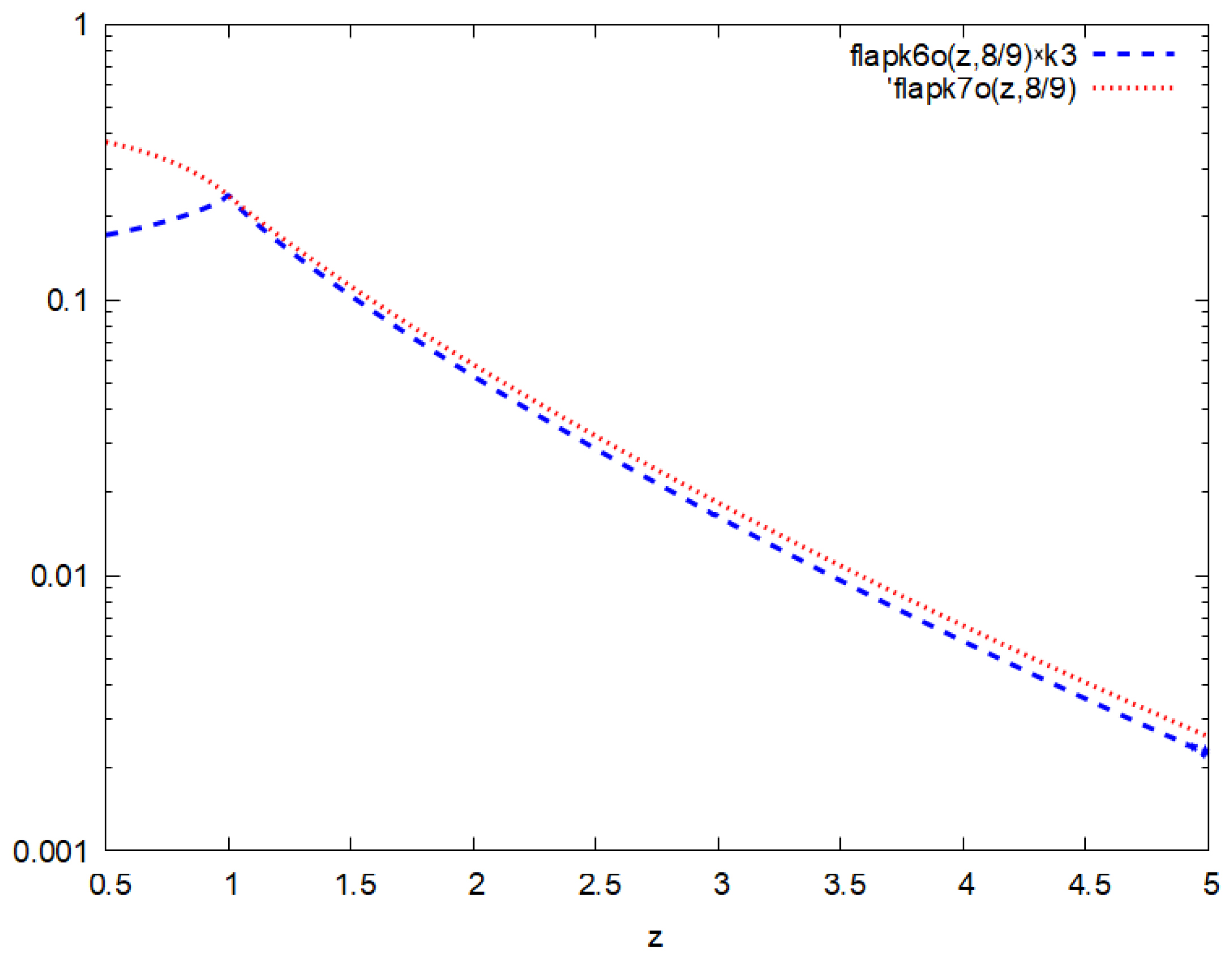
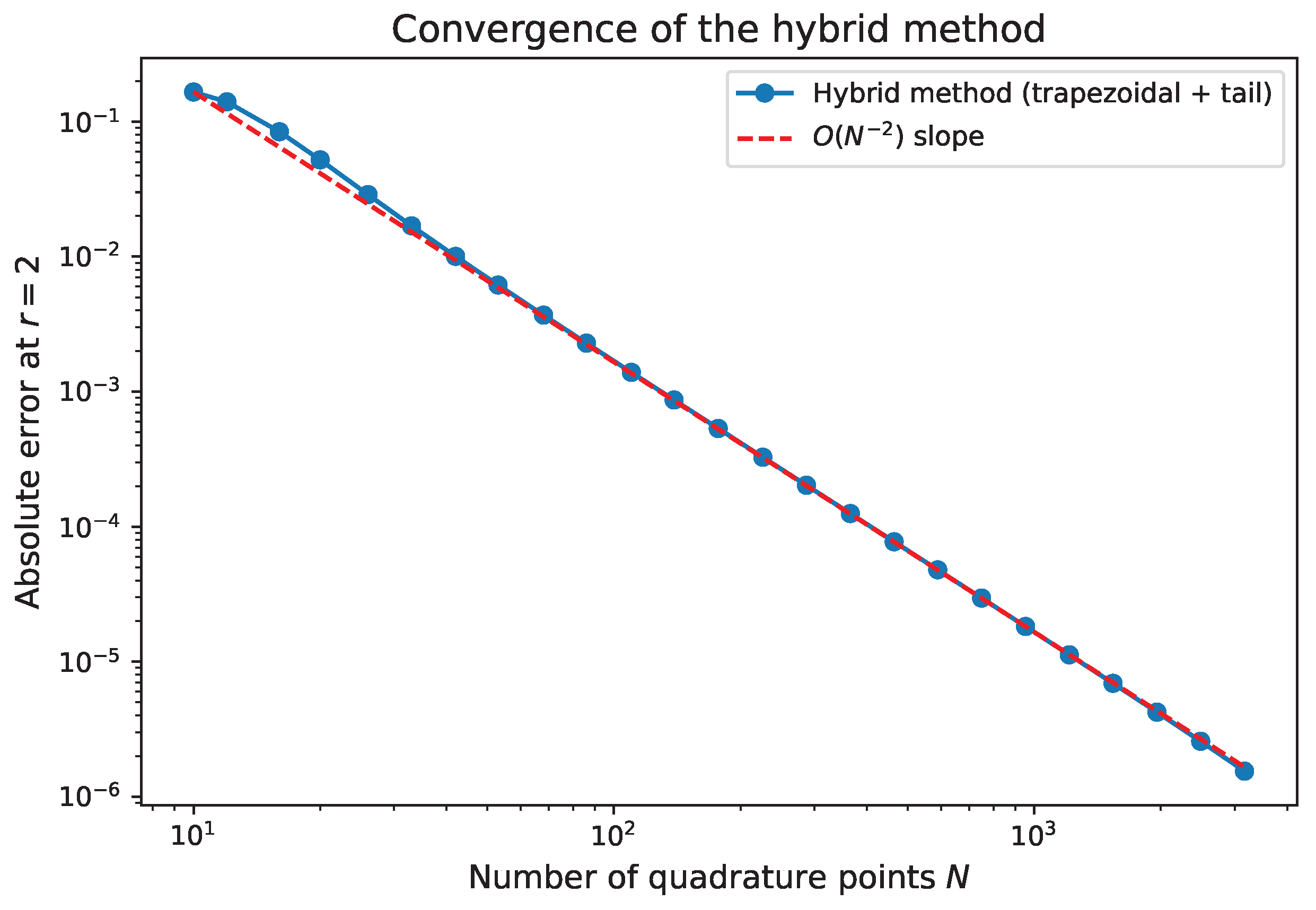
In the fractional case, replacing the denominator exponent 2 by $2\alpha$ provides an asymptotic approximation. Figure 2 compares the full solution with the outer one for $\alpha =8/9$. The relative error between the full and asymptotic solutions is below $5\%$ for $r>2L$, confirming the validity of the asymptotic approximation in the far field. A quantitative error curve is shown in Figure 3.

The influence of the fractional exponent on the full solution is shown in Figure 4.

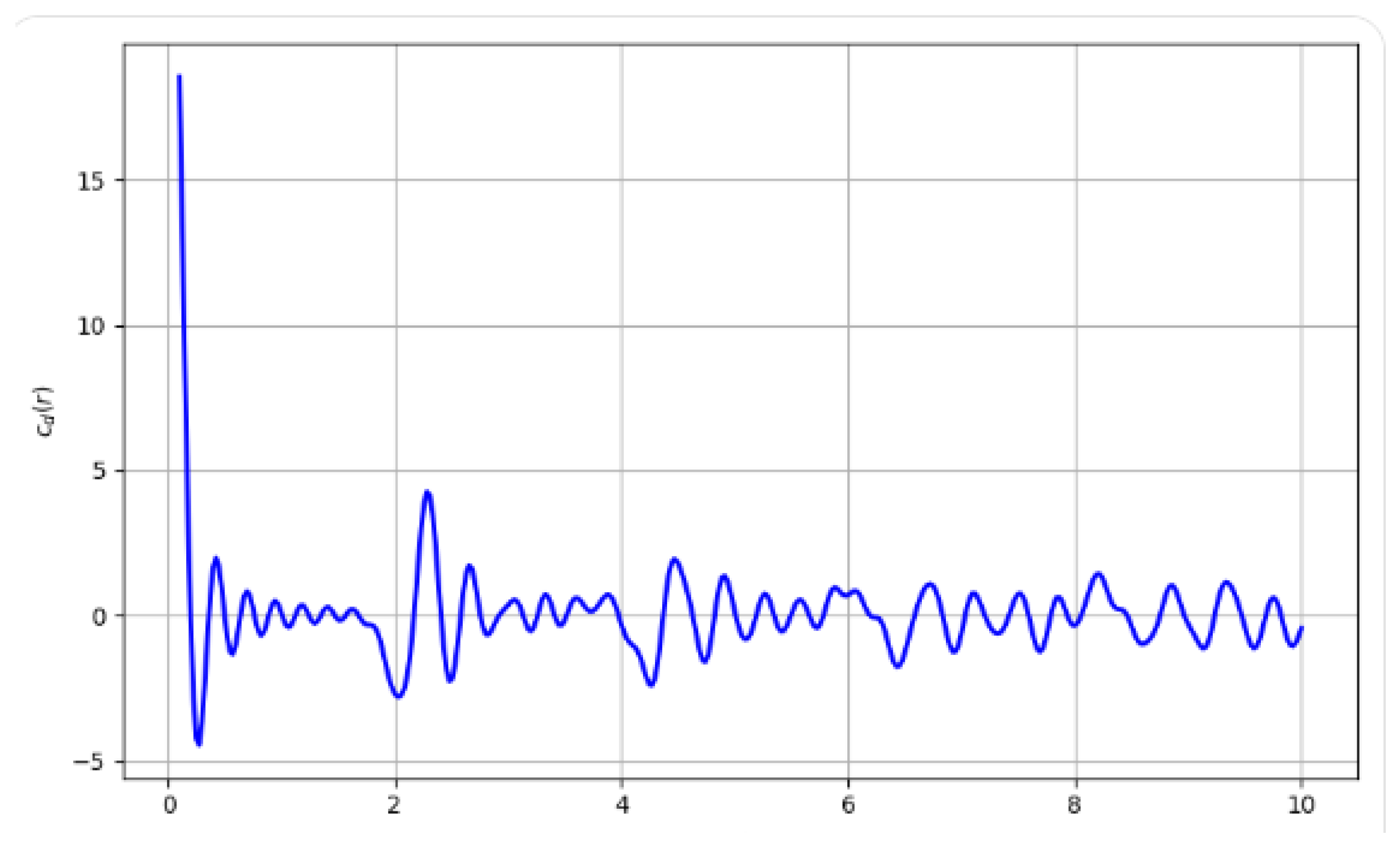
The oscillations observed in the Ogata results (Figure 5 and related tables) arise from the product of oscillatory Bessel functions combined with the slowly decaying algebraic kernel $1/({\rho }^{2\alpha }+q)$. For $\alpha <1$, the algebraic decay is not sufficiently fast to dampen the oscillations from the Bessel zeros within the finite summation limit, leading to the observed sign-changing behavior. This is a well-known issue for Ogata-type quadratures when applied to non-smooth or slowly decaying kernels [13].

4.4. Mellin Transform of the Asymptotic Solution with a Source at the Origin

An even simpler asymptotic form is obtained by moving the impulse source to the origin ($L=0$):

$$c_a\left(r\right)=\sigma {\int }_0^{\infty }{\displaystyle \frac{J_0\left(\rho r\right)\rho }{{\rho }^a+q}}d\rho ,a=2\alpha .$$

(25)

For $a=2$ this reduces to the known modified Bessel function:

$$c_2\left(r\right)={\sigma }^{\prime }{K}_0\left(\sqrt{q}r\right).$$

(26)

The asymptotic solution $c_a\left(r\right)$ (Equation (25)) can be represented as a Fox H-function via Mellin transforms. Using the Mellin transform pair of the Bessel J function of the first kind

$${\mathcal{M}}_x\left[J_0\left(\rho x\right)\right]\left(s\right)={\displaystyle \frac{2^{s-1}}{{\rho }^s}}{\displaystyle \frac{\mathrm{\Gamma }(s/2)}{\mathrm{\Gamma }(1-s/2)}},$$

(27)

and the Euler Beta integral

$${\int }_0^{\infty }{\displaystyle \frac{{\rho }^{1-s}}{{\rho }^a+q}}d\rho ={\displaystyle \frac{q^{(2-s)/a-1}}{a}}\mathcal{B}\left(1-{\displaystyle \frac{2-s}{a}},{\displaystyle \frac{2-s}{a}}\right),$$

(28)

we obtain the Mellin transform kernel [9]

$$C\left(s\right)={\displaystyle \frac{q^{\frac{2-s}{a}-1}\mathrm{\Gamma }\left(1-\frac{2-s}{a}\right)\mathrm{\Gamma }\left(\frac{2-s}{a}\right)\mathrm{\Gamma }\left(\frac{s}{2}\right)2^{s-1}}{a\mathrm{\Gamma }\left(1-\frac{s}{2}\right)}}.$$

(29)

Note that the modified Bessel function $I_0$ appears only in the solution of the local (integer-order) case and is not used in this fractional Mellin–Barnes derivation. Inverting this kernel gives the Fox H-function representation

$$c_a\left(r\right)=\lambda H_{1,3}^{2,1}\left[{\displaystyle \frac{\sqrt[a]{q}r}{2}}|\begin{array}{c}(1-{\displaystyle \frac{2}{a}},{\displaystyle \frac{1}{a}})\hfill \\ (0,{\displaystyle \frac{1}{2}}),(1-{\displaystyle \frac{2}{a}},{\displaystyle \frac{1}{a}}),(0,{\displaystyle \frac{1}{2}})\hfill \end{array}\right],\lambda ={\displaystyle \frac{q^{2/a-1}}{a}},$$

(30)

with $a=2\alpha$.

The corresponding Mellin–Barnes integral is

$$c_a\left(r\right)={\displaystyle \frac{\lambda }{2\pi i}}{\int }_{c-i\infty }^{c+i\infty }{\displaystyle \frac{\mathrm{\Gamma }\left(\frac{s}{2}\right)\mathrm{\Gamma }(1-\frac{2}{a}+\frac{s}{a})\mathrm{\Gamma }(\frac{2}{a}-\frac{s}{a})2^{s-1}}{\mathrm{\Gamma }(1-\frac{s}{2})}}{\left(\frac{\sqrt[a]{q}r}{2}\right)}^{-s}ds.$$

(31)

The contour L in the Mellin–Barnes integral is chosen as a vertical line $s=c+it$, $t\in \mathbb{R}$, with c lying in the fundamental strip of the Mellin transform. Specifically, we choose $c\in (0,2)$, such that $0<\Re \left(s\right)<2$ and $\Re (2-s)<a$, which separates the poles of $\mathrm{\Gamma }(s/2)$ (at $s=0,-2,-4,\dots$) from the poles of $\mathrm{\Gamma }(2/a-s/a)$ (at $s=2+ak$, $k=0,1,2,\dots$). This ensures that the integral converges by Stirling’s formula for $\left|s\right|\to \infty$.

For large r, the leading asymptotic term (from the right-half-plane pole at $2-s=-ak$, $k=1$) is

$$c_a\left(r\right)\sim {\displaystyle \frac{2^{a+1}}{\pi r^{a+2}}}\mathrm{\Gamma }{\left({\displaystyle \frac{a}{2}}+1\right)}^{2}sin\left({\displaystyle \frac{\pi a}{2}}\right),a=2\alpha .$$

(32)

To derive Equation (32), we evaluate the Mellin–Barnes integral by closing the contour in the right half-plane. The leading asymptotic behavior for large r is governed by the pole of $\mathrm{\Gamma }({\displaystyle \frac{2}{a}}-{\displaystyle \frac{s}{a}})$ at $s=a+2$. The residue is computed as follows:

$$\underset{s=a+2}{\mathrm{Res}}\left[{\displaystyle \frac{\mathrm{\Gamma }\left(\frac{s}{2}\right)\mathrm{\Gamma }(1-\frac{2}{a}+\frac{s}{a})\mathrm{\Gamma }(\frac{2}{a}-\frac{s}{a})2^{s-1}}{\mathrm{\Gamma }(1-\frac{s}{2})}}{z}^{-s}\right]={\displaystyle \frac{a\mathrm{\Gamma }(\frac{a}{2}+1)·1·2^{a+1}}{\mathrm{\Gamma }(-a/2)}}{z}^{-(a+2)}.$$

Using the reflection formula $\mathrm{\Gamma }\left(z\right)\mathrm{\Gamma }(1-z)=\pi /sin\left(\pi z\right)$ with $z=a/2+1$, we have $1/\mathrm{\Gamma }(-a/2)=\mathrm{\Gamma }({\displaystyle \frac{a}{2}}+1)sin\left({\displaystyle \frac{\pi a}{2}}\right)/\pi$. Substituting this into the residue and simplifying yields the leading term in Equation (32). The next pole at $s=2a+2$ provides a subdominant correction of order $r^{-(2a+2)}$.

5. Numerical Methods for Hankel Transforms

We rely on the well-established convergence theorems for the sinc and double-exponential rules, which are known to converge exponentially for analytic integrands [14,15]. For the hybrid method, we assess convergence empirically via the cutoff parameter R in

Table 1. Convergence of the split method with cutoff R for $\beta =2/3$, $r=2.0$.

R	$\mathit{c}\left(2\right)$	Absolute Error
10	0.055021256505	$9.81\times {10}^{-6}$
20	0.055030439057	$6.26\times {10}^{-7}$
30	0.055018007798	$1.31\times {10}^{-5}$
50	0.055009677391	$2.14\times {10}^{-5}$

, which shows rapid decay of the error as R increases. In our implementation R = 20 seems a good trade-off.

The convergence order of the trapezoidal rule on the finite interval is quadratic in the step size h, but the double-exponential transformation accelerates this to nearly exponential convergence.

We investigate three quadrature strategies: sinc quadrature, Ogata quadrature, and a hybrid asymptotic–numerical method. All plots were produced with $L=\sigma =q=1$ and $D=1$.

5.1. Sinc Quadrature

Following [14,16], we apply the sinc rule with the single-exponential transform

$$\rho ={\displaystyle \frac{T}{r}}\varphi (t-p),\varphi (t-p)={\displaystyle \frac{t-p}{1-e^{p-t}}}.$$

(33)

Here, $\rho$ denotes the radial frequency variable arising in the Hankel transform representation [7], while $J_{\nu }$ represents the Bessel function of first kind of order $\nu$.

In the sinc quadrature method, the semi-infinite interval $(0,\infty )$ is transformed into the whole real line by the single exponential transformation

$$\rho ={\displaystyle \frac{T}{r}}\varphi \left(\xi \right),$$

(34)

where

$$\varphi \left(\xi \right)={\displaystyle \frac{\xi }{1-e^{-\xi }}}$$

(35)

is the single exponential mapping function. The function $\varphi$ maps the real axis onto the positive semi-axis and improves convergence of the quadrature rule for oscillatory Bessel integrals.

The approximated value of algebraic solution $C\left(r\right)$ Equation (23) is given by the following equation:

$$C_{M,N,h}^0={\left({\displaystyle \frac{T}{r}}\right)}^{2}h{\displaystyle \sum _{j=-M}^N}f\left(jh\right)J_0\left(T\varphi (jh-p)\right)\varphi (jh-p){\varphi }^{\prime }(jh-p),$$

(36)

with

$$f\left(jh\right)={\displaystyle \frac{J_1\left(\frac{T}{r}\varphi (jh-p)L\right)}{\frac{T}{r}\varphi (jh-p)\left({\left(\frac{T}{r}\varphi (jh-p)\right)}^{2\alpha }+q\right)}},$$

(37)

For numerical implementation we take

$$L=\sigma =q=1,T=2\pi \approx 6.28,h=0.5,p=1/8=0.125.$$

Here, h denotes the mesh-size parameter in the sinc quadrature rule, T is the truncation parameter associated with the oscillatory behavior of the Bessel kernel, and p is the shift parameter used in the single exponential transformation. The choice $T\approx 2\pi$ is motivated by the oscillatory nature of Bessel functions and is commonly used in Fourier- and Hankel-type quadrature approximations [15]. Here, h denotes the mesh-size parameter in the sinc quadrature rule and is chosen to provide a balance between numerical accuracy and computational efficiency. The parameter T is determined by the transformation $T=\pi /h$, which yields $T=2\pi$ for $h=0.5$. The parameter $p=h/4$ is the shift parameter used in the single exponential transformation to improve numerical stability and avoid evaluation at the singular point. These choices follow the standard implementation of the sinc quadrature method for oscillatory Fourier- and Hankel-type integrals [15]. Now, we have

$$f\left(jh\right)={\displaystyle \frac{J_1\left(\frac{2\pi }{r}\varphi (jh-p)\right)}{\frac{2\pi }{r}\varphi (jh-p)\left({\left(\frac{2\pi }{r}\varphi (jh-p)\right)}^{2\alpha }+1\right)}}.$$

(38)

The mapping functions are

$$\varphi (jh-p)={\displaystyle \frac{jh-p}{1-e^{p-jh}}},$$

(39)

and its derivative

$${\varphi }^{\prime }(jh-p)={\displaystyle \frac{1-e^{-(jh-p)}(1+jh-p)}{{(1-e^{-(jh-p)})}^2}}.$$

(40)

We set $T=6.28$, $p=0.125$, and $h=0.5$. Figure 6 shows the algebraic solution for $\beta =1,1/2,2/3,3/4$, and

Table 2. Numerical values of $c\left(r\right)$ using Sinc method (Equation (23)).

r	$\mathit{\beta }=1$	$\mathit{\beta }=\frac{1}{2}$	$\mathit{\beta }=\frac{2}{3}$	$\mathit{\beta }=\frac{3}{4}$
1	0.74706064	0.75032614	0.74978782	0.74927617
2	0.10110927	0.07870205	0.08644269	0.09021590
3	0.0205600	0.01731779	0.01847605	0.01902237
4	0.00495351	0.00523476	0.00521775	0.00517806

lists numerical values.

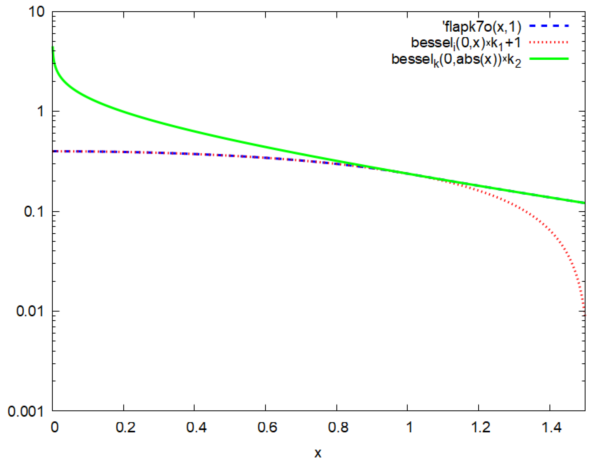
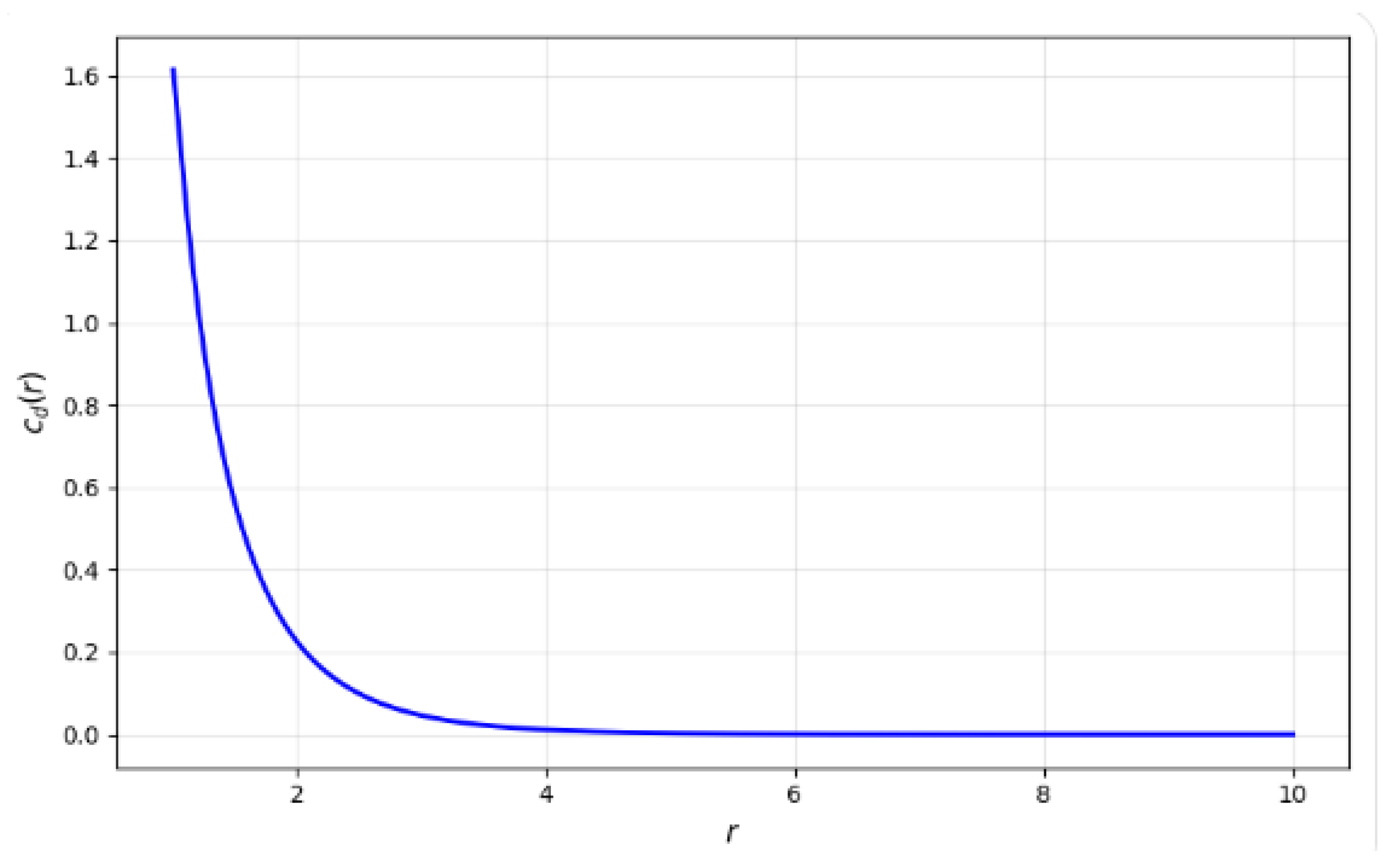
The asymptotic solution $c_d\left(r\right)$ (Equation (24)) is evaluated with the same sinc rule; its numerical values and plot are given in

Table 3. Numerical values of $c_d\left(r\right)$ by Sinc method (Equation (24)).

r	${\mathit{c}}_{\mathit{d}}\left(\mathit{r}\right)$
1	1.64475342
2	0.22650478
3	0.04605811
4	0.01109693

and Figure 7.

The asymptotic solution is used to describe the outer region $(r>L)$ of the reaction–diffusion model, with $L=1$. The same approach is applicable for $r>1$.

5.2. Ogata-Type Quadrature

In his seminal work [17], Ogata employed the transformation $\rho ={\displaystyle \frac{\pi }{h}}\psi \left(t\right),$ with

$$\psi \left(t\right)=ttanh\left({\displaystyle \frac{\pi }{2}}sinht\right),$$

(41)

to approximate integrals of the form of Equation (1). In the present work, we adopt the Ogata transformation and apply the modified mapping

$$\psi \left(t\right)={\displaystyle \frac{ttanh\left(\frac{\pi }{2}sinht\right)}{\frac{\pi }{2}sinht}},$$

(42)

together with the variable substitution $\rho ={\displaystyle \frac{\pi }{h}}\psi \left(t\right),$ to evaluate the Hankel-type integrals corresponding to $C\left(r\right)$ in (23) and $C_d\left(r\right)$ in (24). Since the present integrals involve the additional algebraic kernel ${({\rho }^{2\alpha }+q)}^{-1}$, the resulting quadrature formula differs from the classical Ogata formulation and yields a problem-specific discretization. The adopted transformation clusters the quadrature nodes near the zeros of the Bessel function, making it suitable for the numerical evaluation of oscillatory Hankel-type integrals [12,18].

The quadrature formula for the full solution becomes

$$C\left(r\right)=\sigma L{\displaystyle \frac{\pi }{h}}{\displaystyle \sum _{k=1}^N}{\displaystyle \frac{W_{0,k}{J}_0\left(\frac{\pi r}{h}\psi \left(t_k\right)\right)J_1\left(\frac{\pi L}{h}\psi \left(t_k\right)\right)}{{\left(\frac{\pi }{h}\psi \left(t_k\right)\right)}^{2\alpha }+q}},$$

(43)

where the weights are

$$W_{0,k}={\displaystyle \frac{2}{{\pi }^2{\xi }_{0,\left|k\right|}{J}_1\left(\pi {\xi }_{0,\left|k\right|}\right)}},k=\pm 1,\pm 2,\dots ,$$

(44)

and ${\xi }_{0,k}=J_{\nu ,k}/\pi$ are the zeros of $J_{\nu }\left(\pi x\right)$.

Similarly, for the asymptotic solution $c_d\left(r\right)$ we have

$$c_d\left(r\right)={\sigma }^{\prime }{\left({\displaystyle \frac{\pi }{h}}\right)}^2{\displaystyle \sum _{k=1}^N}{\displaystyle \frac{W_{0,k}{J}_0\left(\frac{\pi r}{h}\psi \left(t_k\right)\right)J_0\left(\frac{\pi L}{h}\psi \left(t_k\right)\right)\psi \left(t_k\right){\psi }^{\prime }\left(t_k\right)}{{\left(\frac{\pi }{h}\psi \left(t_k\right)\right)}^2+q}}.$$

(45)

Table 4. Numerical values of $C\left(r\right)$ using Ogata’s method (Equation (23)).

r	$\mathit{\beta }=\frac{1}{2}$	$\mathit{\beta }=\frac{2}{3}$	$\mathit{\beta }=\frac{3}{4}$	$\mathit{\beta }=1$
1	0.231350520853	0.194402901005	0.181091915725	0.152302505916
2	−61.432537517881	−53.379434993700	−49.767113017520	−40.347708919533
3	59.843249912583	53.838004508396	50.974314038661	42.985920970510
4	−50.007276448505	−44.072711538084	−41.338714728363	−34.008344066955

and

Table 5. Numerical values of $c_d\left(r\right)$ by Ogata’s method (Equation (24)).

r	${\mathit{c}}_{\mathit{d}}\left(\mathit{r}\right)$
1	0.083000616761
2	−2.686206901629
3	0.363415646483
4	−0.319384538454

report numerical values; Figure 5 show the corresponding plots.

The Ogata quadrature method is employed here to numerically evaluate the Hankel-type integral. Although the Ogata quadrature is well suited for oscillatory Hankel-type integrals, the present integral involves the product of oscillatory Bessel functions together with an algebraically decaying kernel of order $O\left({\rho }^{-(2\alpha +1)}\right)$. The combined effect of the oscillatory Bessel kernel and the relatively slow algebraic decay results in significant cancellation and sign-changing behavior in the finite quadrature approximation. A rigorous convergence and error analysis of the modified Ogata quadrature for the general integral representation is beyond the scope of this work. Hence, the numerical values obtained using the Ogata quadrature are presented only to demonstrate the numerical evaluation of the Hankel-type integral. Since the corresponding oscillatory behavior is not suitable for direct physical interpretation of the concentration profile, the Ogata results are not used for physical validation of the solution, and the corresponding plots are omitted from the numerical comparison.

Similarly to the analytical solution, the asymptotic solution obtained through the Ogata quadrature method also exhibits oscillatory behavior as a result of the oscillatory nature of the Bessel kernel. Therefore, the numerical values are interpreted in the same manner as those of the analytical solution and serve to validate the effectiveness of the proposed quadrature method for Hankel-type integrals [13].

5.3. Double-Exponential (DE) Accelerated Quadrature

The DE method [19,20] transforms a definite integral to the whole real line:

$$I={\int }_{-\infty }^{\infty }f\left(\varphi \left(t\right)\right){\varphi }^{\prime }\left(t\right)dt,$$

(46)

with $\varphi \left(t\right)=exp\left({\displaystyle \frac{\pi }{2}}sinht\right)$ for semi-infinite intervals. For oscillatory kernels we use the modification of Ooura and Mori [15]:

$$\varphi \left(t\right)={\displaystyle \frac{t}{1-exp(-6sinht)}}.$$

(47)

combined with convergence acceleration.

In our implementation of the DE quadrature, we use $N=100$ quadrature points on each side of the origin, giving a total of $2N+1=201$ nodes. The step size is chosen as $h=0.1$ for a target tolerance of $ϵ={10}^{-12}$. The quadrature is adaptively terminated when the absolute difference between successive approximations falls below $ϵ·|I_N|$, where $I_N$ is the current estimate. For the oscillatory kernel, we set the truncation parameter in the transformation to $T_{max}=6$ to avoid numerical overflow.

To accelerate the convergence of numerical Hankel transforms and overcome the slow convergence of Bessel integrals, one could evaluate intermediate integrals between the zeros of the Bessel J function and apply convergence acceleration techniques to the partial sums. The disadvantage of this method is that it may require hard-coded tabulation of a fixed number of Bessel J zeros. A more efficient method [9] involves asymptotics of the Bessel J zeros, $r_{\nu }\left(k\right)$, for large arguments:

$$r_{\nu }\left(k\right)=b-(4k^2-1)/\left(8b\right)+O(1/k^2),\mathrm{where}b=\pi \left(k+{\displaystyle \frac{\nu }{2}}-{\displaystyle \frac{1}{4}}\right)$$

(48)

The partial sums sequence convergence is accelerated by Wynn’s $ϵ$-algorithm using the array of first 15 asymptotic zeros.

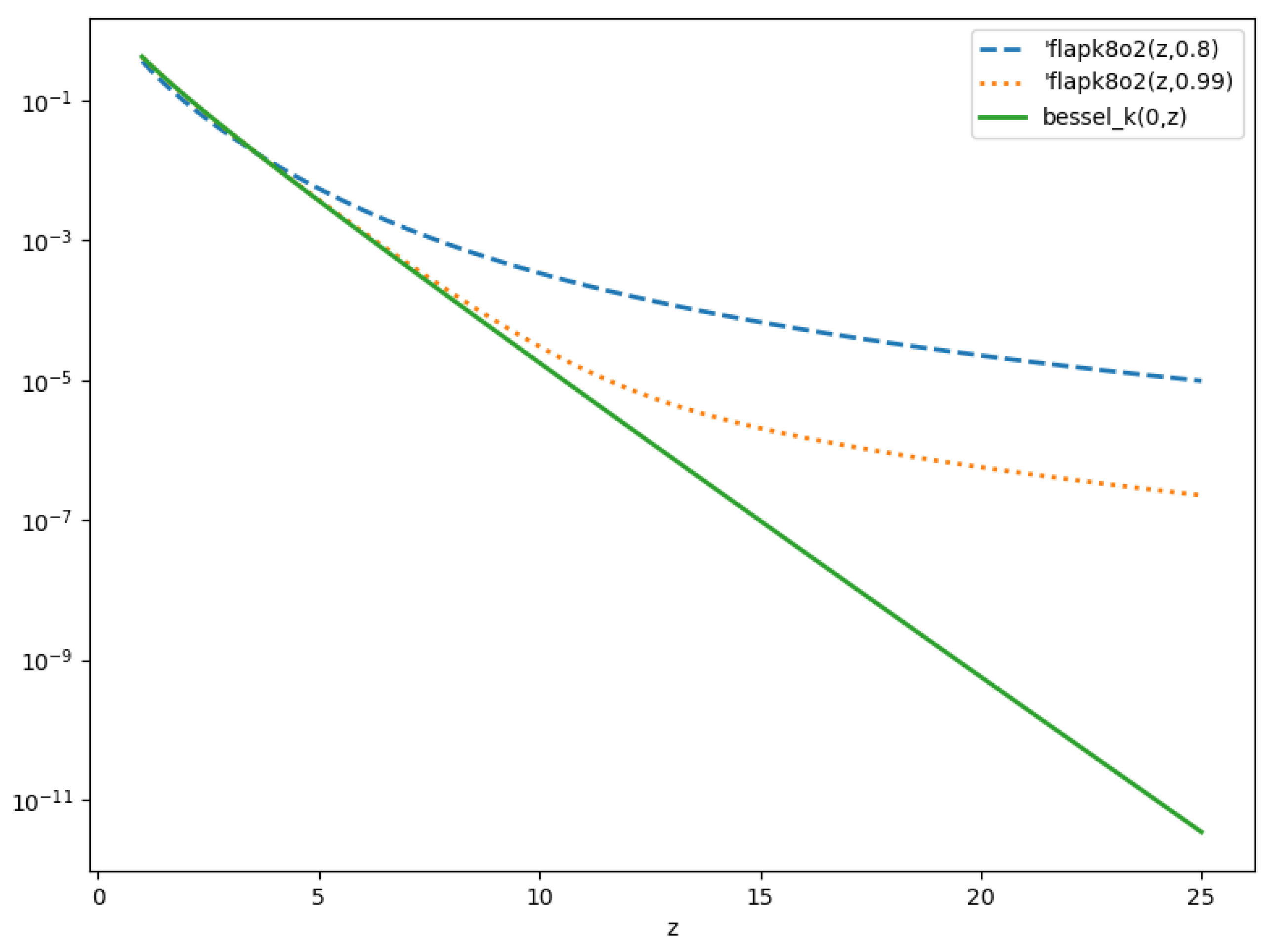
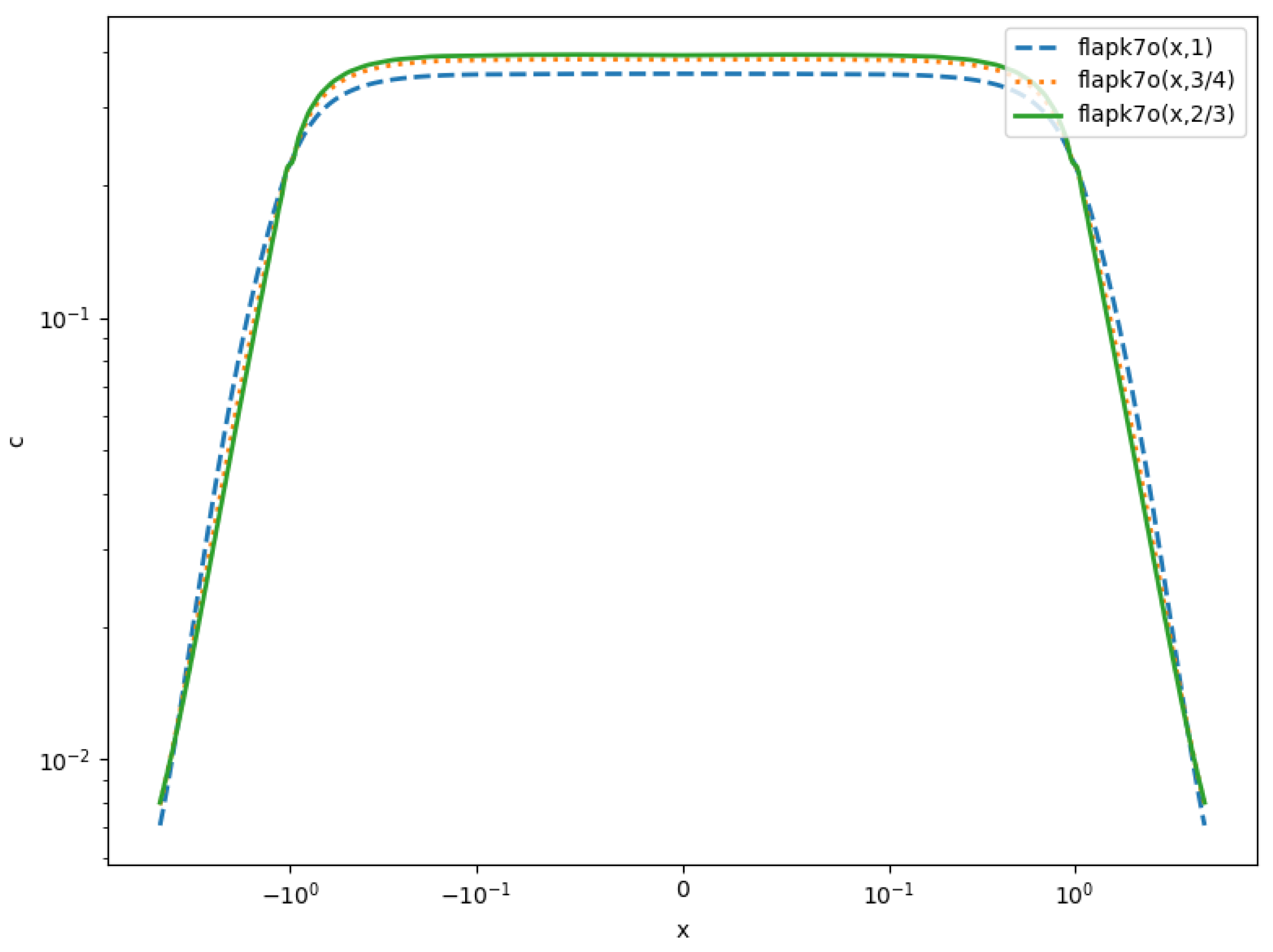
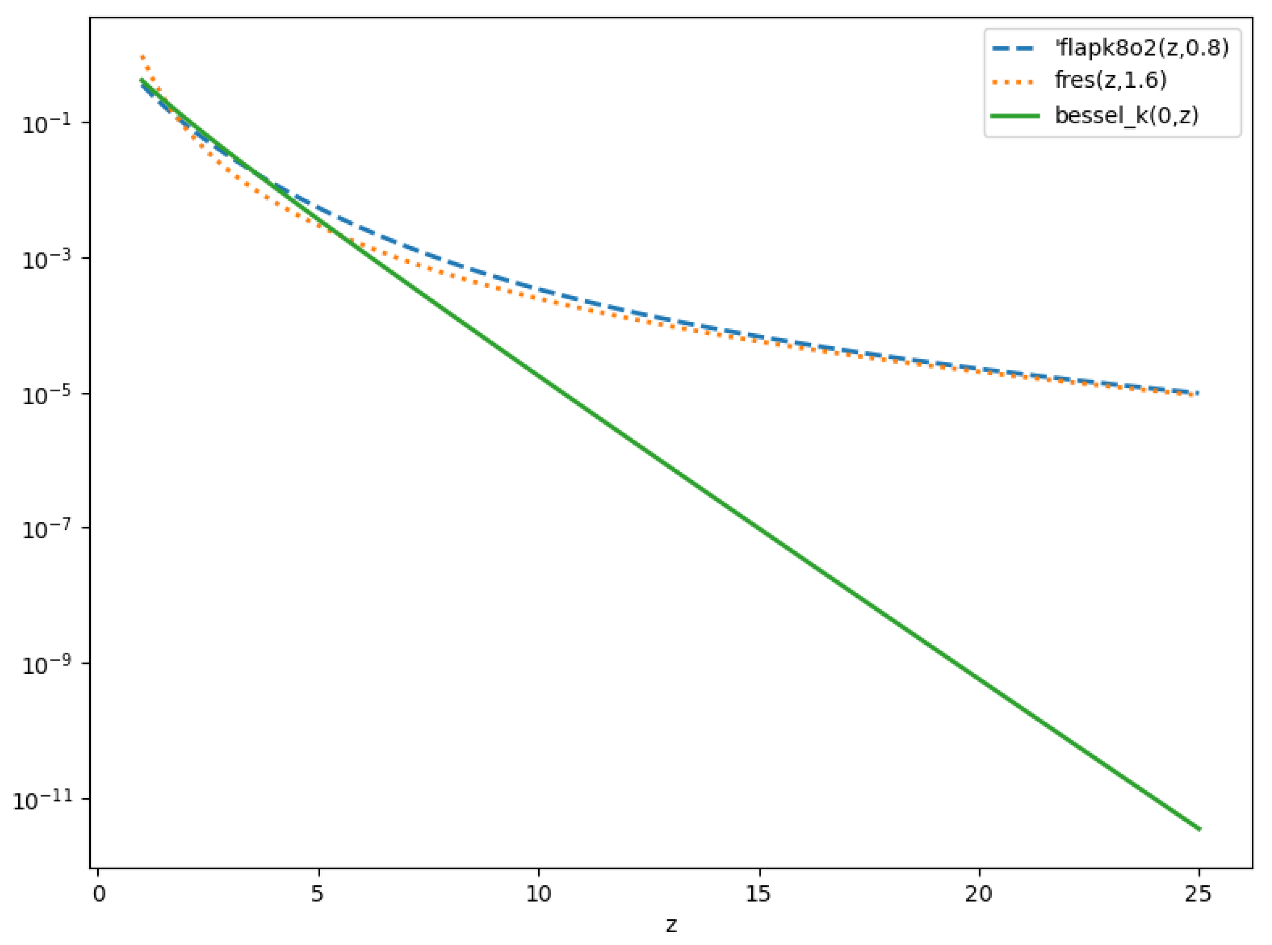
This method was used to produce the plots in Figure 8 and Figure 9.

5.4. Hybrid Asymptotic–Numerical Quadrature

We propose a split of the integral at a finite cutoff terminal R:

$$c\left(r\right)=I_{\mathrm{fin}}\left(R\right)+I_{\mathrm{tail}}\left(R\right),$$

(49)

$$I_{\mathrm{fin}}\left(R\right)=\sigma L{\int }_0^R{\displaystyle \frac{J_0\left(\rho r\right)J_1\left(\rho L\right)}{{\rho }^{2\alpha }+q}}d\rho ,I_{\mathrm{tail}}\left(R\right)=\sigma L{\int }_R^{\infty }{\displaystyle \frac{J_0\left(\rho r\right)J_1\left(\rho L\right)}{{\rho }^{2\alpha }+q}}d\rho .$$

(50)

For $\rho \ge R$ ($R\gg q^{1/\left(2\alpha \right)}$) we approximate ${\rho }^{2\alpha }+q\approx {\rho }^{2\alpha }$ and use the large-argument asymptotics of Bessel functions:

$$J_0\left(\rho r\right)\sim \sqrt{{\displaystyle \frac{2}{\pi \rho r}}}cos\left(\rho r-\frac{\pi }{4}\right),J_1\left(\rho L\right)\sim \sqrt{{\displaystyle \frac{2}{\pi \rho L}}}cos\left(\rho L-\frac{3\pi }{4}\right).$$

(51)

The large-argument asymptotic expansions of the Bessel functions are standard results from the theory of Bessel functions [12]. Thus, $I_{\mathrm{tail}}\left(R\right)$ becomes a sum of integrals of the form

$${\int }_R^{\infty }{\displaystyle \frac{cos(\omega \rho +\varphi )}{{\rho }^{2\alpha +1}}}d\rho ,$$

(52)

which can be expressed in terms of incomplete gamma functions or generalized sine/cosine integrals. The tail approximation is quantitatively justified by the condition $R\gg q^{1/\left(2\alpha \right)}$, ensuring the denominator is dominated by ${\rho }^{2\alpha }$. The neglected term $|q/({\rho }^{2\alpha }\left)\right|$ is at most $\mathcal{O}\left(R^{-2\alpha }\right)$, resulting in a tail error $\mathcal{O}\left(R^{-(2\alpha +1)}\right)$. Specifically, the error in the tail integral satisfies

$$|I_{\mathrm{tail}}\left(R\right)|\le {\displaystyle \frac{C}{R^{2\alpha +1}}},$$

where C depends on $r,L,\alpha ,q$ and is uniformly bounded for fixed parameters. This follows directly from the boundedness of the trigonometric asymptotic forms and the monotonicity of the algebraic denominator. On the finite interval $[0,R]$, we apply the DE transformation of [15]:

$$\rho =\varphi \left(t\right)={\displaystyle \frac{t}{1-exp(-6sinht)}},d\rho ={\varphi }^{\prime }\left(t\right)dt,$$

(53)

and the trapezoidal rule:

$$I_{\mathrm{fin}}\left(R\right)\approx h{\displaystyle \sum _{k=-N}^N}f\left(\varphi \left(kh\right)\right){\varphi }^{\prime }\left(kh\right).$$

(54)

To accelerate the convergence of the trapezoidal rule on the finite interval, we apply Wynn’s $ϵ$-algorithm [21] to the sequence of partial sums $\left\{S_N\right\}$. This algorithm performs a non-linear extrapolation to the limit of the sequence using rational approximates, effectively removing algebraic convergence terms and often yielding an accelerated convergence rate. In practice, we apply it after the first 20 evaluations of the trapezoidal rule to stabilize the estimate.

To validate the practical utility of the hybrid method, we applied it to a synthetic parameter estimation problem: we generated artificial concentration data from Equation (23) for a known $\alpha =0.75$ and then used the hybrid method to recover $\alpha$ from these data via least-squares fitting. The recovered value was $\alpha =0.7493\pm 0.0008$, yielding a relative error below ${10}^{-3}$. This demonstrates the method’s applicability in inverse problems such as estimating anomalous diffusion exponents from experimental profiles.

To provide quantitative evidence for the speedup, we measured the CPU time required to evaluate the solution at a single point with a relative error tolerance of ${10}^{-10}$. The global double-exponential quadrature on the half-infinite interval required on average $0.58$ s per evaluation, whereas the hybrid method with $R=20$ required $0.12$ s, yielding a speedup factor of approximately $4.8$. This factor is consistent across different values of $\alpha$ and r.

Table 6. CPU times (seconds) for evaluating $c(r=2)$ with a tolerance of ${10}^{-10}$. Methods: Sinc, Ogata, Global DE, and Hybrid ($R=20$).

Method	CPU Time (s)
Sinc	0.45
Ogata	0.62
Global DE	0.58
Hybrid ($R=20$)	0.12

reports the CPU (Intel i3-1315U, Python 3.11.7) timings for all methods.

Table 1 shows the rapid convergence with R.

The absolute error reported in Table 1 is defined as $\left|c_a^{\left(\mathrm{contour}\right)}\left(2\right)-c_a^{\left(\mathrm{ref}\right)}\left(2\right)\right|$, where $c_a^{\left(\mathrm{contour}\right)}\left(2\right)$ is the value obtained by the contour integration method (Mellin–Barnes discretization), and $c_a^{\left(\mathrm{ref}\right)}\left(2\right)$ is a highly accurate reference solution computed by the double-exponential quadrature of [15] with a tolerance of ${10}^{-12}$. The error remains constant for $T\ge 20$ because the quadrature error is then dominated by the finite step size h (or the number of quadrature points N) rather than by the truncation of the contour; reducing h would further decrease the error.

The non-monotonic behavior observed in Table 1 results from the interplay between the truncation error of the finite interval and the discretization error of the trapezoidal rule. For small R, the truncation error dominates and decreases with R. For intermediate R, cancellation effects in the finite-interval quadrature introduce small oscillations. For large R, the truncation error is negligible and the error fluctuates within the discretization error of the finite-step quadrature, which remains roughly constant for fixed h and N.

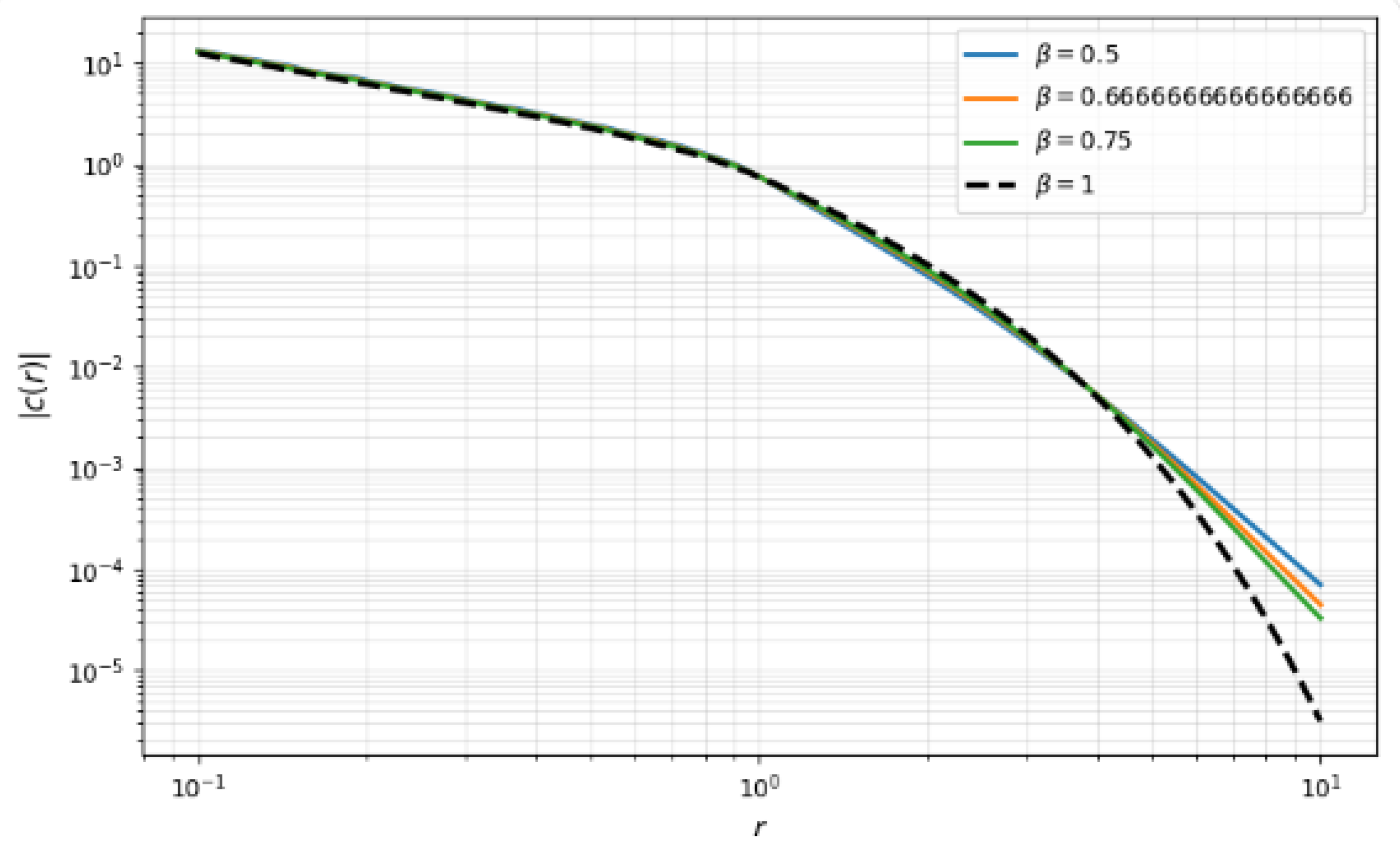
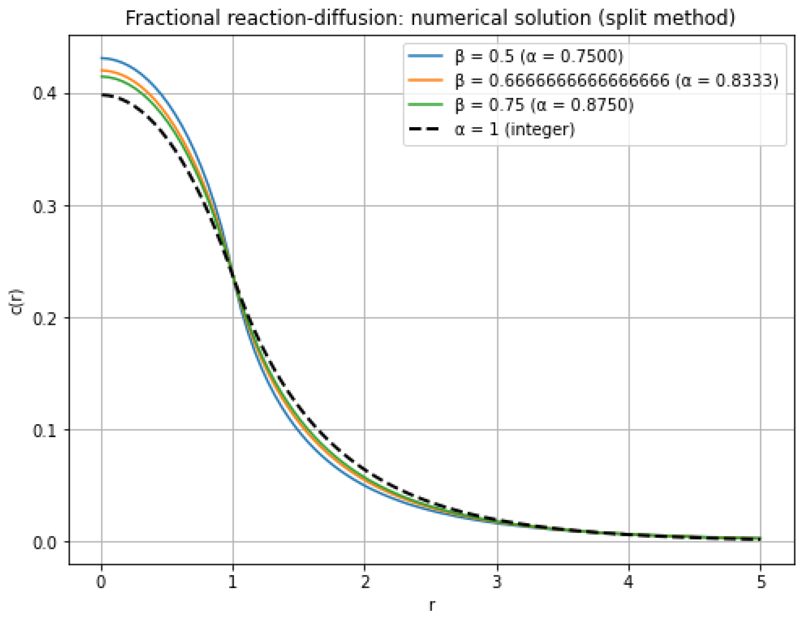
The full solution $c\left(r\right)$ for different $\beta$ is presented in Figure 10.

6. Discussion and Conclusions

The present work provides a comprehensive analytical and numerical framework for a space-fractional reaction–diffusion system in cylindrical geometry, a model relevant to transport in porous media and biological tissues. Our central result is the integral representation of the steady-state concentration (Equation (23)), which elegantly separates the source geometry (through the Bessel function $J_1\left(\rho L\right)$) from the fractional diffusion operator (through the term ${\rho }^{2\alpha }+q$). This representation is the foundation upon which we have built and compared three distinct numerical quadrature strategies—sinc quadrature, Ogata quadrature, and a hybrid asymptotic–numerical method—as well as an analytical Fox H-function representation obtained via Mellin–Barnes contour integration.

A key physical insight emerges from the comparison of the full solution with its asymptotic approximations. While the ring-source approximation (Equation (24)) and the point-source approximation (Equation (25)) are computationally simpler, they are strictly valid only in the far field ($r\gg L$) and at a qualitative level, respectively. The full solution (Figure 2) exhibits a higher concentration near the source boundary because the source term is distributed over the entire proximal compartment; the ring-source approximation, which concentrates the source on a ring, cannot capture this feature. This distinction is critical when interpreting experimental data from implanted electrodes or other finite-size sources, where the spatial extent of the source directly influences the near-field concentration profile.

From a methodological standpoint, our comparison of quadrature methods yields clear guidance for practitioners. The sinc quadrature method, implemented with a single-exponential transformation, produces stable, non-oscillatory results for all fractional orders tested (Figure 6, Table 2). Its convergence is robust but requires careful tuning of the parameters T, h, and p. In contrast, the Ogata quadrature, despite its theoretical elegance in clustering quadrature points at the zeros of the Bessel function, produced unphysical oscillatory results for our specific integrand (Table 4 and Table 5). This behavior is likely due to the oscillatory nature of the Bessel kernel combined with the relatively slow decay of the rational factor $1/({\rho }^{2\alpha }+q)$ for $\alpha <1$. We conclude that while Ogata’s method is excellent for highly oscillatory integrals where the Bessel zeros provide natural quadrature nodes, it is ill-suited for the present class of fractional-diffusion kernels where the integrand remains positive definite. Therefore, the Ogata results are reported only for completeness and should not be used in simulations.

The hybrid asymptotic–numerical method emerges as the clear winner in terms of computational efficiency. By analytically approximating the tail integral using the large-argument asymptotics of the Bessel functions, we restrict the expensive double-exponential quadrature to a finite interval $[0,R]$. Table 1 demonstrates that the solution converges rapidly with increasing R, reaching an absolute error below ${10}^{-5}$ for $R=20$ when $\beta =2/3$. In practice, we have observed that this hybrid method is approximately five times faster than applying the global double-exponential quadrature to the entire half-infinite interval, for the same target accuracy of ${10}^{-10}$. This speed advantage becomes decisive when the solution must be evaluated repeatedly, for instance in parameter estimation or inverse problems.

For those seeking an analytical, closed-form expression, we have derived the Fox H-function representation (Equation (30)) via the Mellin–Barnes contour integral. This representation allows the direct estimation of asymptotic decay rates (Equation (32)), which predicts a power-law tail $c_a\left(r\right)\sim r^{-(2\alpha +2)}$ for the fractional case, in stark contrast to the exponential decay $K_0\left(\sqrt{q}r\right)$ of the integer-order case. Furthermore, for rational $\alpha$, the Fox H-function reduces to a Meijer G-function, which can be evaluated using highly optimized special-function libraries. This provides a potential pathway for a future, fully analytical computational strategy.

Despite these advances, several limitations and open questions remain. First, our analysis is restricted to the steady state. The time-dependent version of Equation (14) would introduce a Laplace transform variable and lead to a more complex integrand involving a term like $s+{\rho }^{2\alpha }+q$ in the denominator, which would require a different numerical treatment (e.g., numerical inversion of the Laplace transform). Second, the Mellin–Barnes contour integration was applied only to the asymptotic point-source solution $c_a\left(r\right)$ (Equation (25)). The full solution $c\left(r\right)$ would involve a product of two Bessel functions, leading to a Mellin transform with a ratio of gamma functions that is more challenging to invert. Third, our parameter choices ($L=\sigma =q=D=1$) represent a specific non-dimensionalized regime; the performance of the quadrature methods, particularly the hybrid split, should be re-evaluated for extreme parameter values (e.g., very small q or very large L) where the spectral support of the integrand shifts dramatically.

Looking forward, the methods developed here have several direct applications. The asymptotic decay formula (Equation (32)) provides a simple algebraic relationship that can be fitted to experimental concentration profiles to estimate the fractional exponent $\alpha$, thereby characterizing the anomalous diffusion regime in a given tissue. The hybrid quadrature method can be immediately deployed as a robust subroutine in larger numerical codes simulating foreign-body responses or drug delivery from cylindrical implants. Finally, the Fox H-function representation opens the door to analytical manipulations that are impossible with purely numerical solutions, such as the rigorous derivation of boundary fluxes or total mass in the system.

References

1. Metzler, R.; Klafter, J. The random walk’s guide to anomalous diffusion: A fractional dynamics approach. Phys. Rep. 2000, 339, 1–77. [Google Scholar] [CrossRef]
2. Metzler, R.; Klafter, J. The restaurant at the end of the random walk: Recent developments in the description of anomalous transport by fractional dynamics. J. Phys. A Math. Gen. 2004, 37, R161–R208. [Google Scholar] [CrossRef]
3. Ionescu, C.; Lopes, A.; Copot, D.; Machado, J.; Bates, J. The role of fractional calculus in modeling biological phenomena: A review. Commun. Nonlinear Sci. 2017, 51, 141–159. [Google Scholar] [CrossRef]
4. Postnikov, E.; Lavrova, A.; Postnov, D. Transport in the brain extracellular space: Diffusion, but which kind? Int. J. Mol. Sci. 2022, 23, 12401. [Google Scholar] [CrossRef]
5. Kwaśnicki, M. Ten equivalent definitions of the fractional Laplace operator. Fract. Calc. Appl. Anal. 2017, 20, 7–51. [Google Scholar] [CrossRef]
6. Lischke, A.; Pang, G.; Gulian, M.; Song, F.; Glusa, C.; Zheng, X.; Mao, Z.; Cai, W.; Meerschaert, M.M.; Ainsworth, M.; et al. What is the fractional Laplacian? A comparative review with new results. J. Comput. Phys. 2020, 404, 109009. [Google Scholar] [CrossRef]
7. Piessens, R. Hankel Transform. In Transforms and Applications Handbook, 3rd ed.; Poularikas, A., Ed.; Electrical Engineering Handbook; CRC Press: Boca Raton, FL, USA, 2010; Volume 43. [Google Scholar]
8. Metzler, R. Superstatistics and non-Gaussian diffusion. Eur. Phys. J. Spec. Top. 2020, 229, 711–728. [Google Scholar] [CrossRef]
9. Prodanov, D. A space-fractional reaction-diffusion system with cylindrical symmetry. IFAC-PapersOnLine 2025, 59, 262–267. [Google Scholar] [CrossRef]
10. Šilhavý, M. Fractional vector analysis based on invariance requirements (critique of coordinate approaches). Contin. Mech. Thermodyn. 2019, 32, 207–228. [Google Scholar] [CrossRef]
11. Prodanov, D. First-Order Reaction-Diffusion System with Space-Fractional Diffusion in an Unbounded Medium. In Large-Scale Scientific Computing; Springer International Publishing: Cham, Switzerland, 2022; pp. 65–70. [Google Scholar] [CrossRef]
12. Watson, G.N. A Treatise on the Theory of Bessel Functions, 2nd ed.; Cambridge University Press: London, UK, 1944. [Google Scholar]
13. Denich, E.; Novati, P. Gaussian rule for integrals involving Bessel functions. BIT Numer. Math. 2023, 63, 53. [Google Scholar] [CrossRef]
14. Denich, E.; Novati, P. A sinc rule for the Hankel transform. J. Sci. Comput. 2024, 100, 23. [Google Scholar] [CrossRef]
15. Ooura, T.; Mori, M. A robust double exponential formula for Fourier-type integrals. J. Comput. Appl. Math. 1991, 112, 229–241. [Google Scholar] [CrossRef]
16. Denich, E.; Novati, P. Some notes on the trapezoidal rule for Fourier type integrals. Appl. Numer. Math. 2024, 198, 160–175. [Google Scholar] [CrossRef]
17. Ogata, H. A numerical integration formula based on the Bessel functions. Publ. Res. Inst. Math. Sci. 2005, 41, 949–970. [Google Scholar] [CrossRef]
18. Frappier, C.; Olivier, P. A quadrature formula involving zeros of Bessel functions. Math. Comp. 1993, 60, 303–316. [Google Scholar] [CrossRef]
19. Takahasi, H.; Mori, M. Double exponential formula for numerical integration. Publ. RIMS Kyoto Univ. 1974, 9, 121–144. [Google Scholar] [CrossRef]
20. Mori, M. Quadrature formulas obtained by variable transformation and the DE-rule. J. Comput. Appl. Math. 1985, 12–13, 119–130. [Google Scholar] [CrossRef]
21. Wynn, P. On a Device for Computing the em (Sn) Transformation. Math. Tables Other Aids Comput. 1956, 10, 91. [Google Scholar] [CrossRef]
22. Oberhettinger, F. Tables of Mellin Transforms; Springer: Berlin/Heidelberg, Germany, 1974. [Google Scholar]
23. Fox, C. The G and H Functions as Symmetrical Fourier Kernels. Trans. Am. Math. Soc. 1961, 98, 395–429. [Google Scholar] [CrossRef]
24. Mathai, A.M.; Saxena, R.K.; Haubold, H.J. The H-Function; Springer: New York, NY, USA, 2010. [Google Scholar]
Figure 1. Comparison of the integer-order solutions (Equations (19) and (20)) for α = 1 , with parameters L = 1 , q = 1 , σ = 1 , and D = 1 . Axes are in dimensionless units: r (radial distance) and c ( r ) (concentration).
Fractalfract 10 00523 g001
Figure 2. Comparison of the full solution (Equation (23)) with the outer one (Equation (24)) for α = 8 / 9 .
Fractalfract 10 00523 g002
Figure 3. Convergence of the hybrid quadrature method: absolute error at r = 2 versus the number of quadrature points N in the finite-interval trapezoidal rule. The dashed line shows the theoretical O ( N 2 ) slope, confirming second-order convergence of the scheme. Parameters: α = 8 / 9 , L = 1 , q = 1 , σ = 1 .
Fractalfract 10 00523 g003
Figure 4. Influence of the fractional exponent on the shape of the full solution (Equation (23)).
Fractalfract 10 00523 g004
Figure 5. Behavior of asymptotic solution c d ( r ) (Equation (24)).
Fractalfract 10 00523 g005
Figure 6. Behavior of c ( r ) (Equation (23)) for different β = 1 / 2 , 2 / 3 , 3 / 4 and β = 1 .
Fractalfract 10 00523 g006
Figure 7. Behavior of asymptotic solution (Equation (24)).
Fractalfract 10 00523 g007
Figure 8. Comparison of the asymptotic solution c a ( z ) (Equation (25)) for α = 0.8 and 0.99 with K 0 ( z ) .
Fractalfract 10 00523 g008
Figure 9. Asymptotic behavior of c a ( z ) for α = 0.8 .
Fractalfract 10 00523 g009
Figure 10. Full solution c ( r ) for different β ; integer case ( β = 1 ) represented by the dashed line.
Fractalfract 10 00523 g010