Self-Similar Currents and Their Properties Based on the General Theory of Fractal Elements

Abstract

This paper is a first step toward providing answers to the question of whether fractal pattern formation gives rise to power-law (fractional) kinetics and how such kinetics relate to geometric properties such as fractal dimension. The study focuses on Lichtenberg figures produced by high-voltage discharges on wood, a heterogeneous dielectric medium with anisotropic conductivity and variable moisture content. During breakdown, the discharge propagates through branching streamers and carbonization fronts, exhibiting scale-free growth, long-tailed waiting times, and memory effects. The associated current signals are analyzed using the theory of fractal elements developed by Nigmatullin and Chen. This framework allows complex self-similar waveforms to be decomposed into elementary fractal modes characterized by power-law exponents and amplitudes. The results show that the electrical response is governed by fractional dynamics encoded in these modes. However, no direct one-to-one relationship is found between the fractal dimension of the discharge patterns and the kinetic power-law exponents. This decoupling is attributed to the influence of the heterogeneous medium and the percolation pathways through which the discharge propagates.

1. Introduction and Formulation of the Problem

Fractal growth processes often arise in systems governed by anomalous transport, memory effects, and long-range correlations, features that are not adequately described by classical integer-order differential equations and thus by exponential relaxations.

Does fractal pattern formation induce power law (fractional) kinetics [1]? If so, to which parameter, particularly a geometric one, is the power law (fractional) order linked? Is the dimension of the resulting fractal pattern related to the power law (fractional) order? These are the questions that motivated this study illustrating through various experiments that a close link exists between power-law kinetics and fractal pattern formation. The aim is to find methods of modeling fractional dynamics other than fractional models which now show some limitations [2,3].

In this paper, the authors are particularly interested in the formation of Lichtenberg figures during high-voltage discharge on wood surfaces, as this provides a striking example of fractal pattern formation in a heterogeneous dielectric medium [4]. When a wooden substrate—characterized by anisotropic conductivity and variable moisture content—is subjected to electric fields exceeding its breakdown threshold, the discharge propagates as a branching network of streamers and carbonization fronts. These fronts exhibit scale-free growth, long-tailed waiting-time distributions, and memory-dependent propagation, all of which are hallmarks of fractional kinetics.

Experimental observations consistently show that the discharge does not advance with a constant velocity or classical exponential kinetics. This reflects the influence of the wood’s heterogeneous microstructure: local resistivity changes due to carbonization, moisture gradients, and thermal feedback introduce memory effects and non-local interactions that accumulate over time.

But does this formation generate fractional kinetics at the level of the electrical signals that generate them? During high-voltage breakdown on wooden substrates, the formation of Lichtenberg figures is accompanied by complex and highly irregular electrical signals. These current–time signals, recorded during the propagation of the discharge and the carbonization front, exhibit strong fluctuations, burst-like events, intermittency, and long-tailed statistics.

To begin to answer the question of fractional current kinetics, the recent theoretical framework formulated by Nigmatullin and Chen [5] is used here to show the self-similarity of the current signal and to model it. Their general theory of fractal elements, grounded in the self-similarity principle, shows that a complex experimental waveform can be decomposed into a combination of elementary self-similar modes. Each mode is characterized by a power-law scaling exponent and amplitude, jointly capturing the deterministic trend and the stochastic fluctuations present in the signal. This decomposition allows the experimental current trace to be interpreted not as noise superimposed on a smooth trend, but as a structured combination of fractal elements whose scaling indices encode the underlying fractional dynamics. The present paper can therefore be seen as an application of the theory presented in [5] to current signals generated by high-voltage discharges on wood.

In the context of dielectric breakdown in wood, this approach is particularly relevant. While the fractal dimension of Lichtenberg figures has been extensively studied using spatial methods such as box-counting, the present work focuses on the temporal dynamics of the discharge process as recorded in the current signals. These two aspects (spatial geometry and temporal kinetics) are not necessarily equivalent, and our aim is precisely to investigate whether, and if so how, they are related. The fractal elements framework of Nigmatullin and Chen [5] provides a rigorous method for analyzing the self-similarity of time-series data, which is the central object of our study. Using the Nigmatullin–Chen method [5], the current–time data can therefore be analyzed to extract a set of fractional exponents that correspond to the hierarchical and self-similar kinetic processes driving the breakdown. By applying this methodology to current signals recorded during the formation of Lichtenberg figures, we demonstrate that the electrical response itself exhibits fractal and fractional characteristics, and that these characteristics can be quantitatively described through the decomposition framework introduced by Nigmatullin and Chen [5]. The essence of this theory is the decomposition of a complex self-similar signal into a combination of fractal modes governed by a set of power-law exponents. And this idea can be confirmed on many self-similar processes developed in time and space.

The novel contributions of this work are threefold. First, the fractal elements framework of Nigmatullin and Chen [5] is applied to current signals generated by high-voltage discharges on wood, a class of signals that has not previously been analyzed using this methodology. Second, a systematic comparison across nine different board geometries (varying aperture patterns and electrode configurations) is conducted to assess the robustness and reproducibility of the extracted scaling parameters. Third, a physical interpretation of these parameters is provided in the context of percolation-controlled discharge dynamics, and the relationship between spatial fractal geometry and temporal fractional kinetics is critically examined. These results demonstrate that while the structural scale parameter ln(ξ) remains remarkably stable across configurations, the kinetic exponents ν₁ and ν₂ exhibit significant variability, reflecting the sensitivity of the discharge process to sample-specific percolation pathways.

2. Experimental Part and Data Measurements Procedure

The data analyzed in this paper result in the formation of Lichtenberg figures on wooden substrates through the application of high-voltage electrical stress, highlighting the interplay of dielectric breakdown, moisture distribution, and fractal discharge propagation.

Wood, a naturally anisotropic dielectric material, normally exhibits high electrical resistivity. However, its conductivity can be modified by introducing a weak electrolyte at the surface, altering the local dielectric constant and promoting controlled charge migration. Under the influence of a sufficiently high potential difference—typically in the kilovolt range—the electric field across the wood can exceed the material’s breakdown strength, initiating a process analogous to surface dielectric breakdown [6,7].

Once breakdown begins, localized heating causes pyrolysis of cellulose and lignin within the wood fibres. This carbonization lowers the resistivity along the discharge path, creating a positive feedback mechanism: as conductive carbon channels form, the electric field becomes increasingly concentrated in those regions, further expanding the discharge network. This results in the development of tortuous, branching fractal structures, mathematically related to diffusion-limited aggregation and often characterized by a fractal dimension between 1.5 and 1.8 [8,9]. 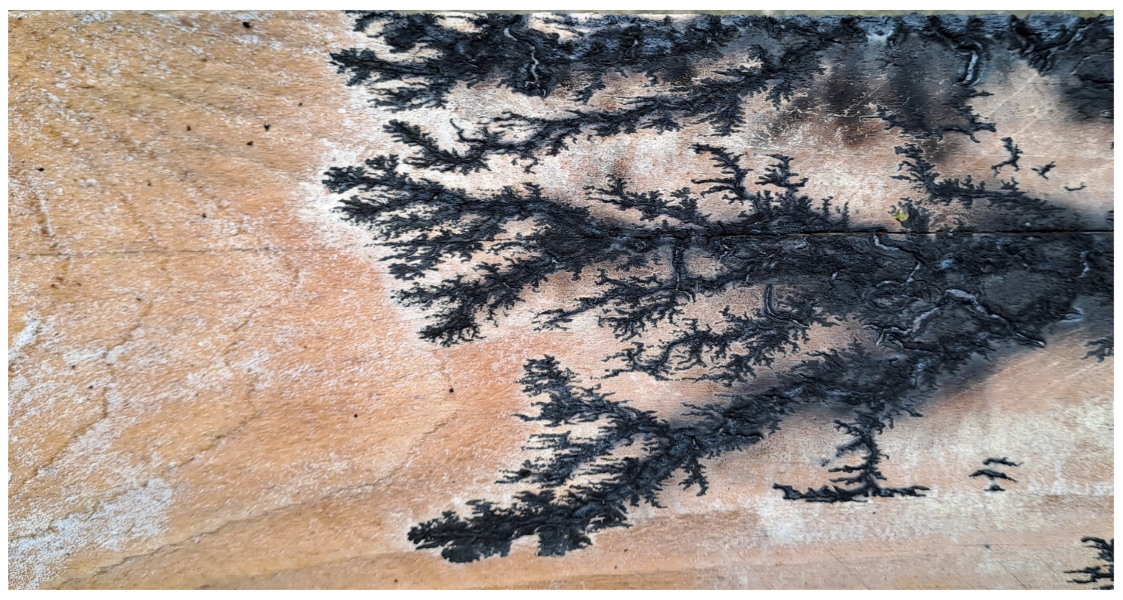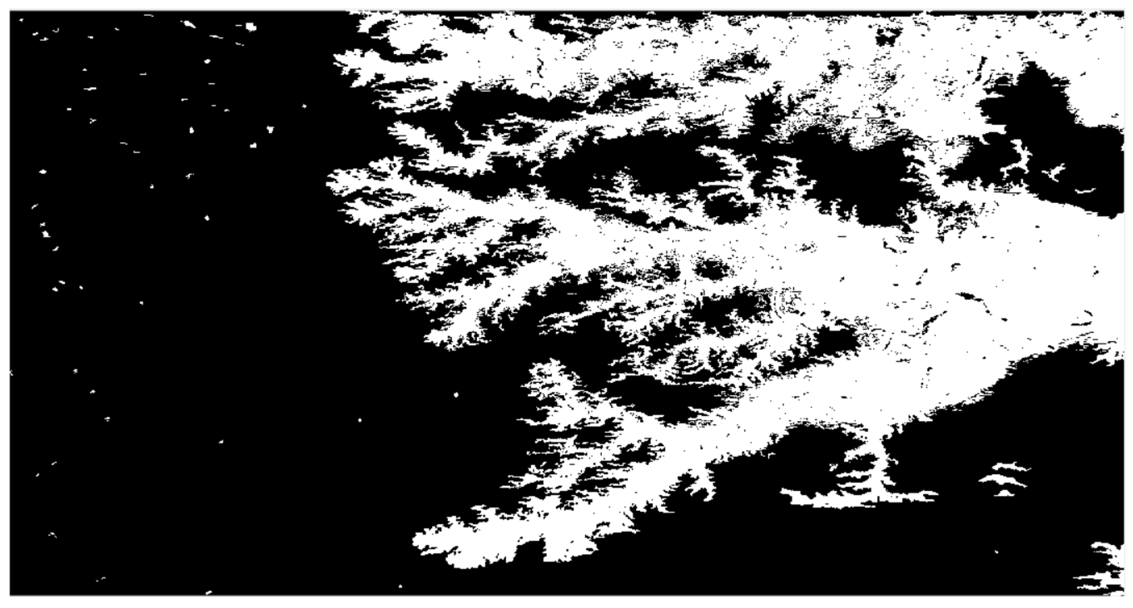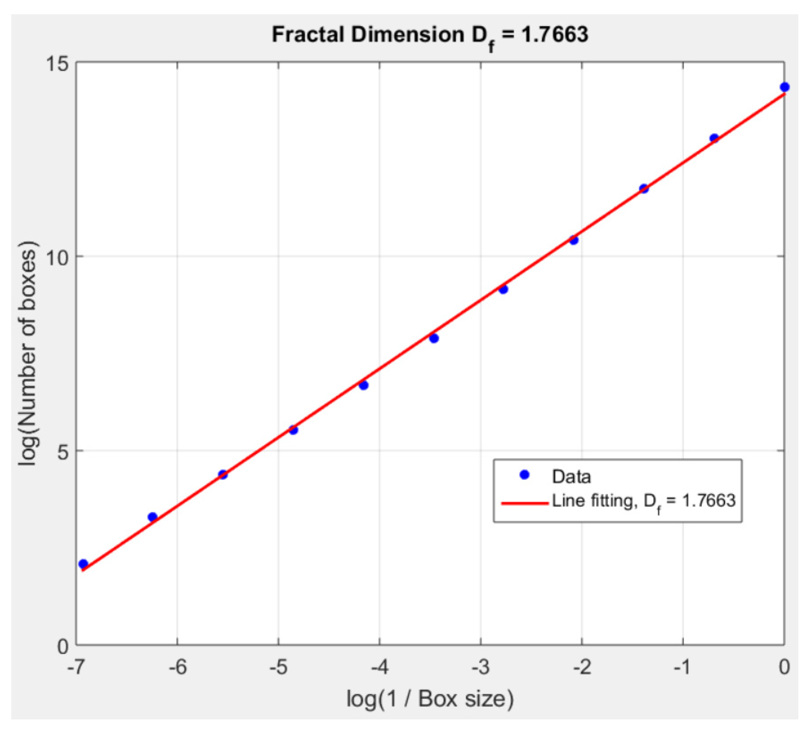This is also the case in this study as shown in Appendix B, in which the analysis of an obtained figure yields a fractal dimension of 1.76.

Electrically, the system behaves as a complex, nonuniform resistive–capacitive network. Transient arcs, microdischarges, and filamentary plasmas propagate stochastically across the surface, guided by variations in grain direction, moisture gradients, ionic concentration, and local defects. These transient arcs generate rapid temperature spikes capable of carbonizing the surface in milliseconds. As the discharge evolves, the branching pattern expands outward from the electrode contact regions, producing characteristic dendritic structures [10,11].

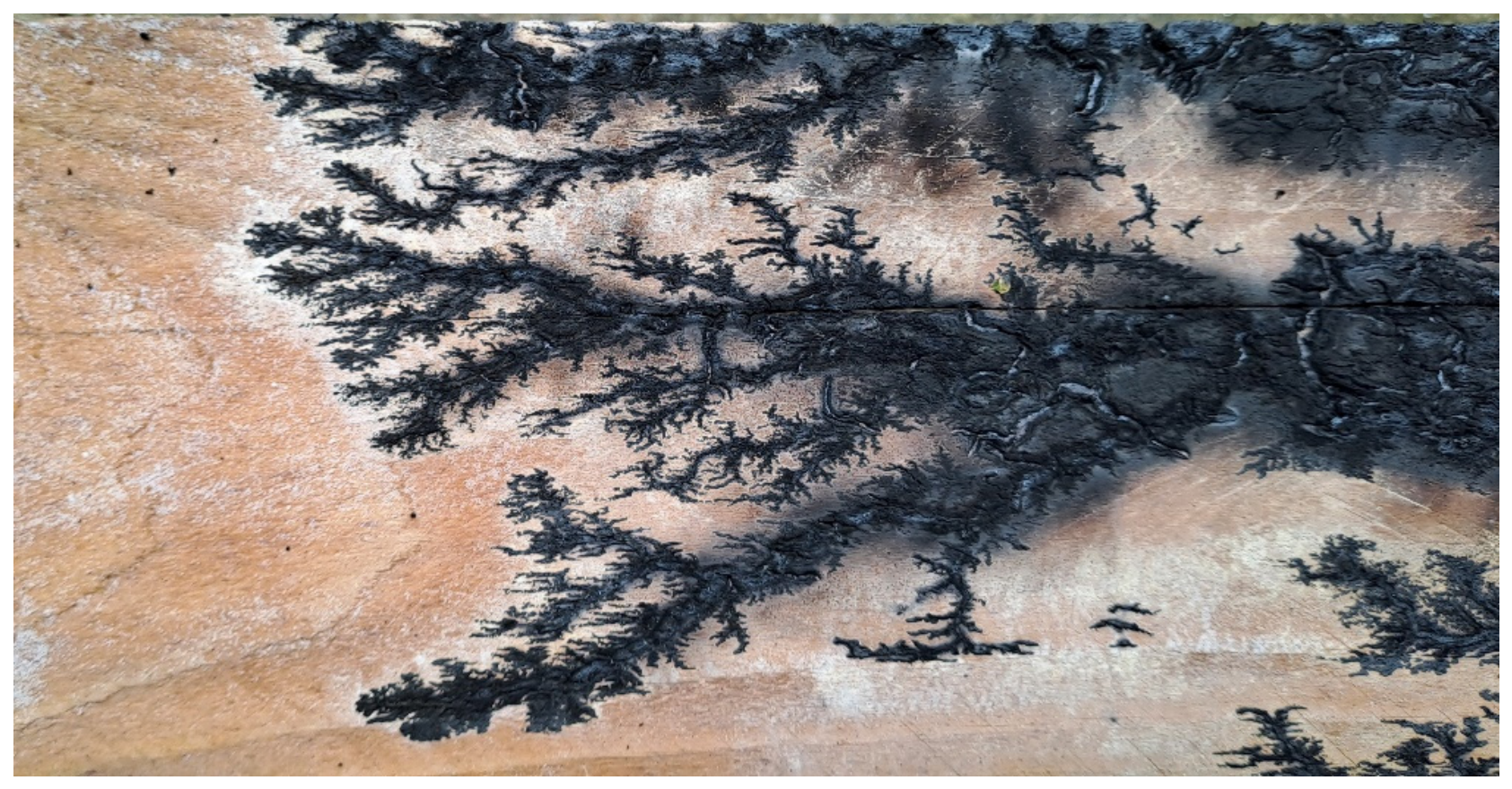
After the high-voltage source is de-energized, as shown by Figure 1, the resulting Lichtenberg figure appears as a network of carbonized fissures embedded in the wood. These patterns are permanent records of the spatial distribution of electrical stress during breakdown and provide a visually striking representation of the underlying physical processes governing fractal discharge formation.

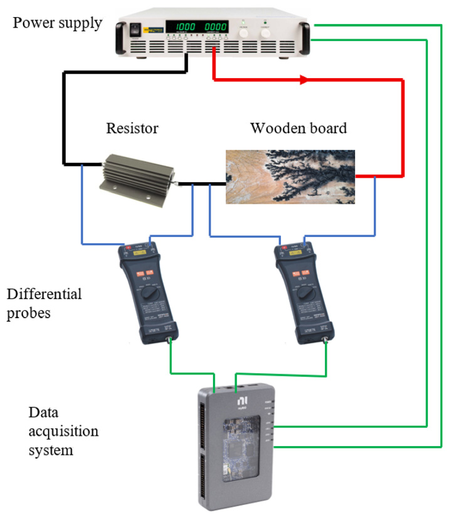
In this paper, the current signals induced by the formation of Lichtenberg figures are analyzed. These signals are obtained using the test bench described in Figure 2. This bench consists of a high-voltage power supply [0 to 2 kV] (Reference DP20H-1-5PH from DSC Electronics, Bonn, Germany) which simultaneously powers a wooden board and a resistor connected in series. The resistor is used as a current sensor. The current and voltage signals across the wooden board are measured simultaneously by the power supply and by differential probes (Reference Gw Instek GDP-050, New Taipei City, Taiwan). These measurements are recorded using an acquisition system (Reference National Instruments MyRio, Austin, TX, USA) with a sampling period of 5 ms.

Table 1. Pictures and numbering of the boards subjected to an electric field.

Board Number	Board Picture
1
2
3
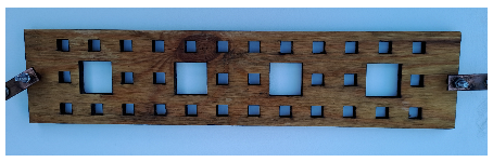
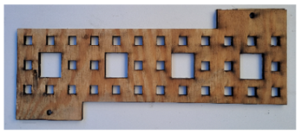
4
5
6
7
8
9

presents a series of pictures documenting the nine wooden boards investigated in this study. Each board was subjected to a similar high-voltage excitation protocol, but with different electrode configurations and surface conditions as the boards already exhibit geometric structures with different degrees of fractality, defined by the pattern and density of square apertures carved into the surface. The aperture patterns serve to influence the percolation pathways available to the discharge. However, the present study does not involve any spatial fractal analysis of the resulting Lichtenberg figures. Our analysis focuses exclusively on the self-similarity of the recorded current signals.

The pictures show that, although the material and global dimensions are similar, the boards differ in two essential aspects:

• The spatial distribution and density of the apertures;
• The locations of the electrode connection points.

These geometric and topological differences condition the range of possible current paths and the ease or difficulty with which percolation occurs. Some boards have exactly the same geometry and, in this case, allow for testing the reproducibility of tests and analyses. This is the case for boards:

-

1, 2 and 5: electrical connection on both ends symmetrically and Sierpinski fractal lattice up to order three;

-

3 and 6: electrical connection on one end on one side, and Sierpinski fractal lattice up to order three;

-

4 and 7: electrical connection on both sides symmetrically and Sierpinski fractal lattice up to order three;

-

8 and 9: electrical connection on both ends symmetrically and Sierpinski fractal lattice up to order four.

All experiments were conducted in ambient environmental conditions (temperature 22 ± 2 °C, relative humidity 45 ± 5%). A 0.1 M sodium bicarbonate solution was applied uniformly to the board surface to promote controlled charge migration. Copper tape electrodes were pressed firmly onto the board surface at the designated contact points. All boards had a thickness of 10 mm. These parameters were kept as consistent as possible across experiments to ensure comparability.

3. Data Processing Procedure

In paper [5], one of the present authors proposed the general theory of fractal elements that can be used to fit a wide class of self-similar (fractal) curves satisfying the condition

$$\begin{array}{c}\left(D_{\xi }-\lambda \right)F\left(z\right)\simeq \epsilon \simeq 0,\\ D_{\xi }F\left(z\right)\stackrel{\mathrm{def}}{=}F\left(z\xi \right).\end{array}$$

(1)

The fractal elements framework proposed by Nigmatullin and Chen [5] differs from classical scaling analysis methods such as Detrended Fluctuation Analysis (DFA) [12,13] or wavelet-based [14] approaches in that it explicitly separates the deterministic trend from the stochastic fluctuations through a decomposition into elementary self-similar modes. While DFA and Hurst exponent [15] estimation provide a single global scaling exponent, the present approach yields a full spectrum of modes with distinct power-law exponents and amplitudes, enabling a more detailed characterization of the hierarchical dynamics underlying the discharge process. This methodology has been successfully applied to various self-similar signals, including photodiode noise and transcendental number sequences, but its application to Lichtenberg discharge currents constitutes, to our knowledge, a novel contribution.

In expression (1), the second line defines the self-similar scaling operator D_ξ that underlines the fractal property of a function F(z). The solution of this simple functional Equation (1) is well-known and can be expressed as

$$\begin{array}{c}F\left(z\right)=z^{\nu }\mathit{Pr}(\mathit{ln}z)=\mathit{exp}(\nu \mathit{ln}(z)\left)\mathit{Pr}(\mathit{ln}z\right),\\ \mathit{Pr}(\mathit{ln}z)={\displaystyle \sum _{k=0}^{K\gg 1}}\left(A{c}_k\mathit{cos}\left(2\pi k({\displaystyle \frac{\mathit{ln}z}{\mathit{ln}\xi }})\right)\right)+A{s}_k\mathit{sin}\left(2\pi k({\displaystyle \frac{\mathit{ln}z}{\mathit{ln}\xi }})\right),\\ \nu =\mathit{ln}(\lambda )/\mathit{ln}\left(\xi \right),D_{\xi }\mathit{Pr}(\mathit{ln}z)=\mathit{Pr}(\mathit{ln}z\xi )=\mathit{Pr}(\mathit{ln}z).\end{array}$$

(2)

However, in many cases this solution is not suitable for the fitting purposes because it leads to large values of the fitting error. In paper [5], other cases were considered, and to achieve acceptable fitting error values even more complex cases can be considered. In the present case it is sufficient to consider the situation with two power-law exponents. The fitting function is written in the form

$$\begin{array}{c}\left(D_{\xi }-{\lambda }_1\right)\left(D_{\xi }-{\lambda }_2\right)F\left(z\right)\simeq \epsilon =0,\\ F\left(z\right)=z^{{\nu }_1}{\mathit{Pr}}_1\left(\mathit{ln}z\right)+z^{{\nu }_2}{\mathit{Pr}}_2\left(\mathit{ln}z\right),\\ {\nu }_{\mathrm{1,2}}=\mathit{ln}\left({\lambda }_{\mathrm{1,2}}\right)/\mathit{ln}\left(\xi \right)\end{array}$$

(3)

In order to fit the function (3) to actual data it is necessary to verify their self-similar (SS) property. Based on the concepts of the fractal elements given in the paper, this general theory can be used to fit a variety of random trends/curves satisfying the SS principle.

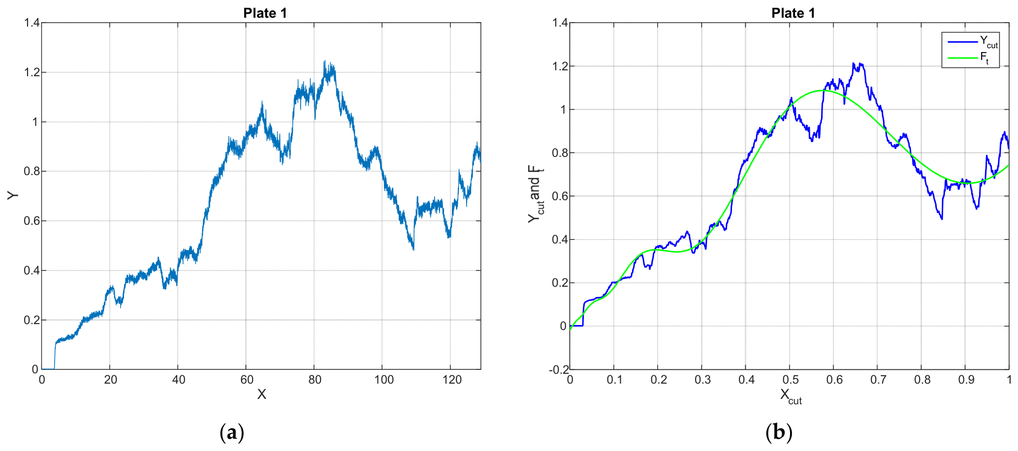
For that purpose, let us take a set of data produced with board n°1 considered with respect to dimensionless time (normalized by 1 s). As shown by Figure 3, these data exhibit clear self-similarity when compressed 10–100 folds.

To complement the visual evidence of self-similarity, we performed a quantitative scaling analysis using Detrended Fluctuation Analysis (DFA) [12,13]. The DFA method computes the fluctuation function $F\left(n\right)$ as a function of window size $n$. A power-law scaling $F\left(n\right)~n^{\alpha }$ indicates self-similarity, with $\alpha >0.5$ signalling long-range correlations. For board 1, we obtained $\alpha \approx 1.38\pm 0.021$ over the scaling range $n\in \left[10, 500\right]$ samples, confirming that the current signal exhibits statistically significant scale invariance. This quantitative result supports the visual observation of self-similarity and justifies the application of the fractal elements decomposition.

The green line shown in Figure 3 demonstrates the fit of this function by means of three power-law functions without log-periodic corrections:

$$\begin{array}{c}Ft\left(x\right)=A_0{x}^{{\nu }_1}+A_1{x}^{\mathit{Re}({\nu }_2)}\mathit{cos}(\mathit{Im}({\nu }_2\left)\mathit{ln}(x\right))+\\ A_2{x}^{\mathit{Re}({\nu }_2)}\mathit{sin}(\mathit{Im}({\nu }_2\left)\mathit{ln}(x\right)).\end{array}$$

(4)

If we compare expression (4) with the more complete expression (3), it can be seen that (4) serves as an initial decomposition of (3) without log-periodic corrections. The satisfactory fitting of the compressed data by expression (4) prompted us to select the following simplified fitting function

$$\begin{array}{c}Ff(x:K,\mathit{ln}(\xi ))=A_1{\left|{\lambda }_1\right|}^{\mathit{ln}(x)/\mathit{ln}\xi }+\\ (+{\left|{\lambda }_2\right|}^{\mathit{ln}(x)/\mathit{ln}\xi }{\sum }_{k=1}^K(A{c}_k^{\left(1\right)}\mathit{cos}\left({\displaystyle \frac{\mathit{arg}({\lambda }_2)+2\pi k}{\mathit{ln}\xi }}\mathit{ln}(x)\right)+\\ A{s}_k^{\left(1\right)}\mathit{sin}\left({\displaystyle \frac{\mathit{arg}({\lambda }_2)+2\pi k}{\mathit{ln}\xi }}\mathit{ln}(x)\right)\left)\right).\end{array}$$

(5)

The log-normal correction for the root λ₁ is omitted based on the structure of the simplified function (4). Expression (5) contains two-nonlinear fitting parameters: number of modes K and the scaling parameter ln(ξ). They can be found from the minimization value of the relative fitting error

$$Err(K,\xi )=\left({\displaystyle \frac{stdev\left(Ycu{t}_3\right(x)-Ff(x;K,\mathit{ln}(\xi \left)\right))}{mean\left(\left|Ycu{t}_3\left(x\right)\right|\right)}}\right)\cdot 100\%.$$

(6)

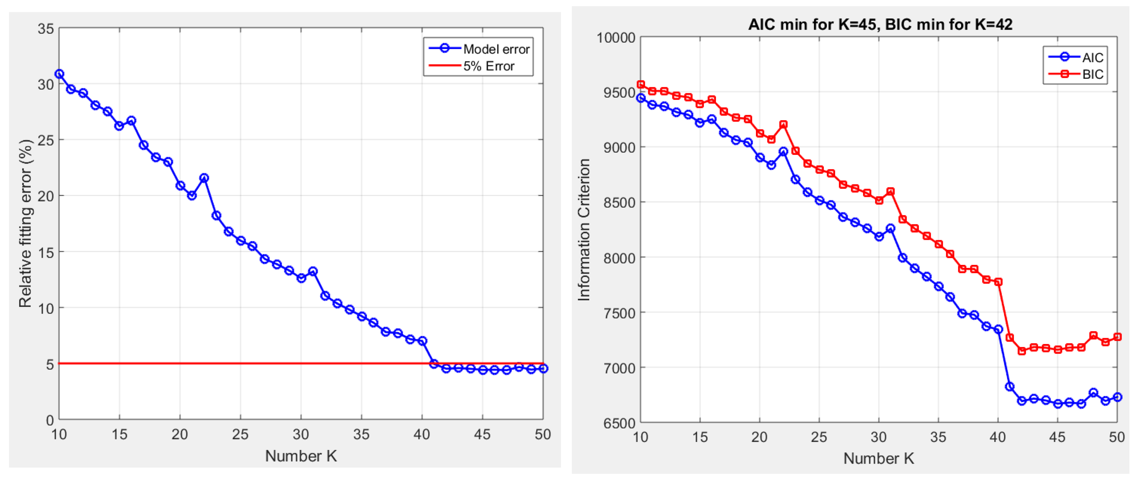
The optimization of the number of modes K follows from the requirement that the value of the relative error be located in the interval (1–5%). The parameter K is therefore gradually increased until the relative error falls below 5%. Concerning the number of power law exponents, three power-law exponents is excessive, while the model with one power-law exponent is not sufficient.

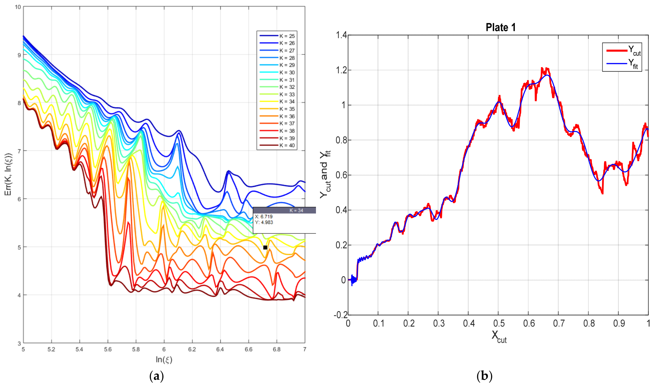
This error is represented in Figure 4 as a function ln(ξ) for several numbers of modes K.

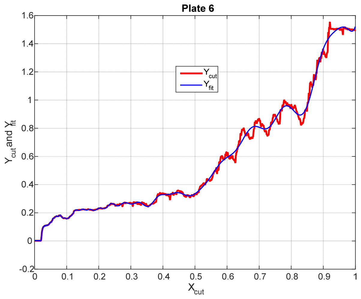
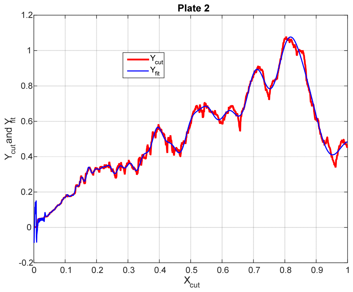
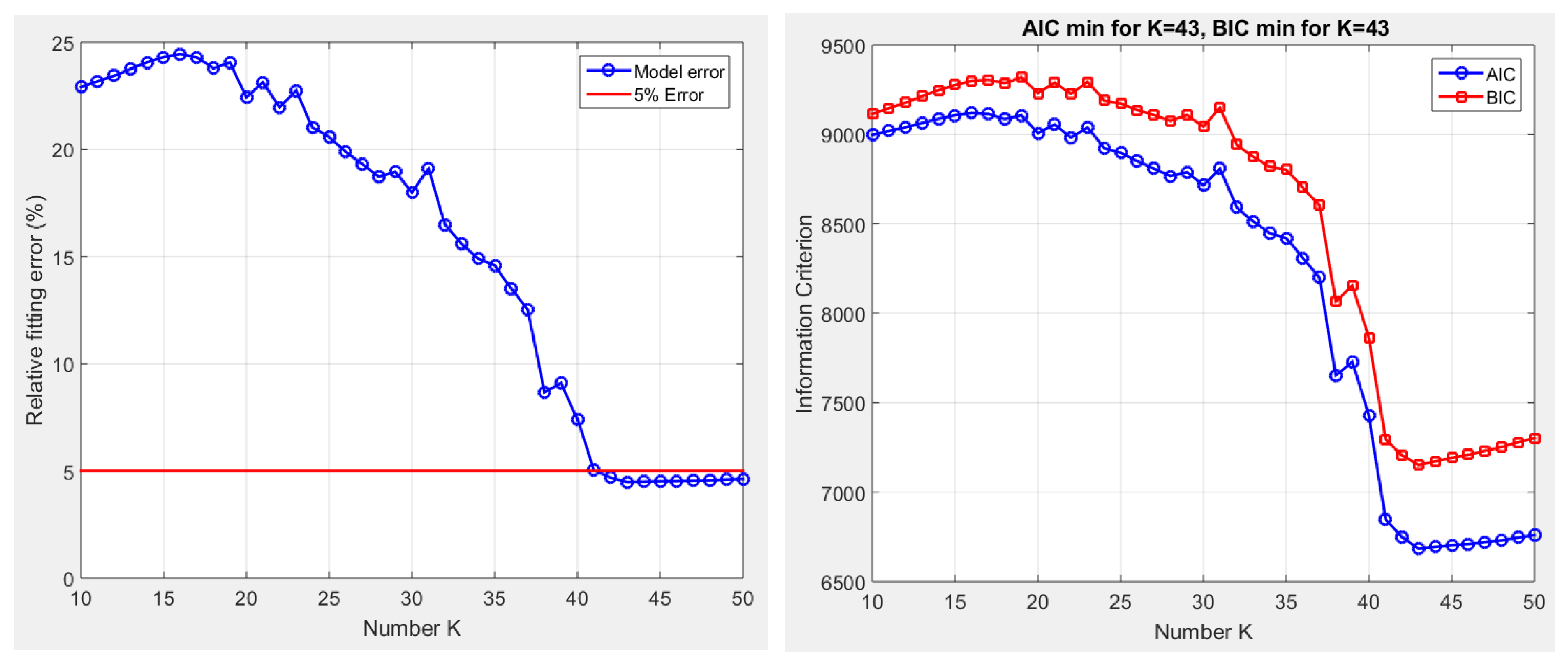
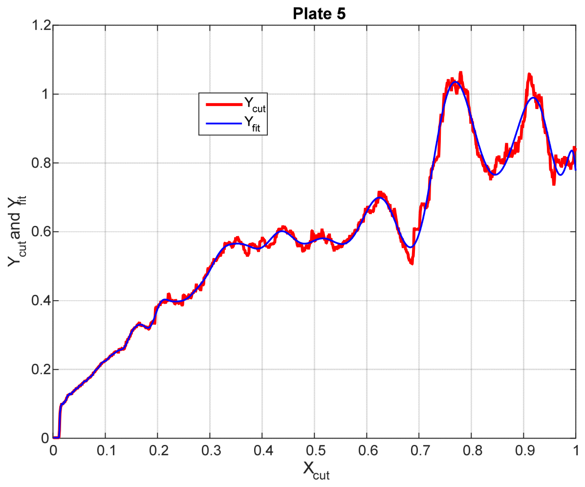
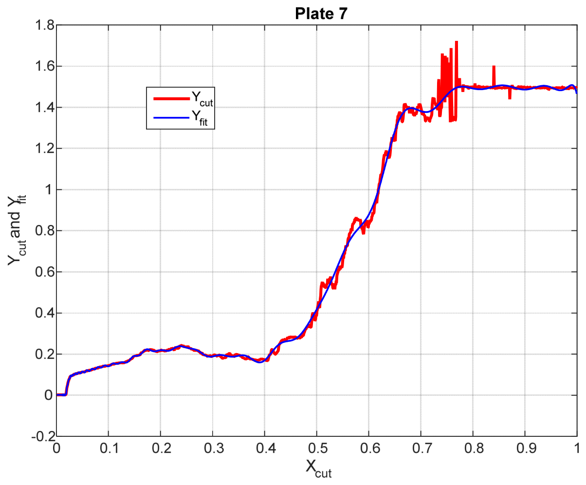
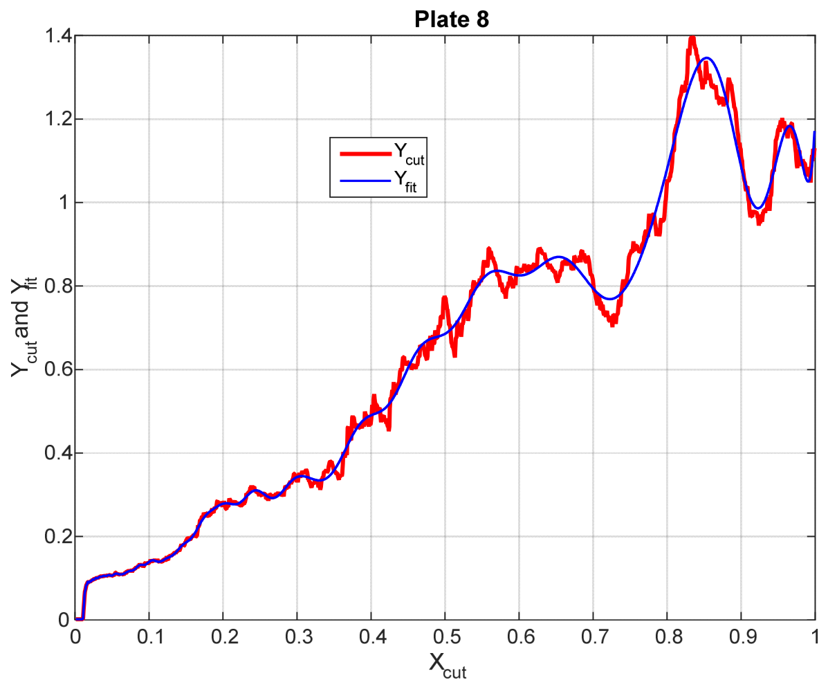
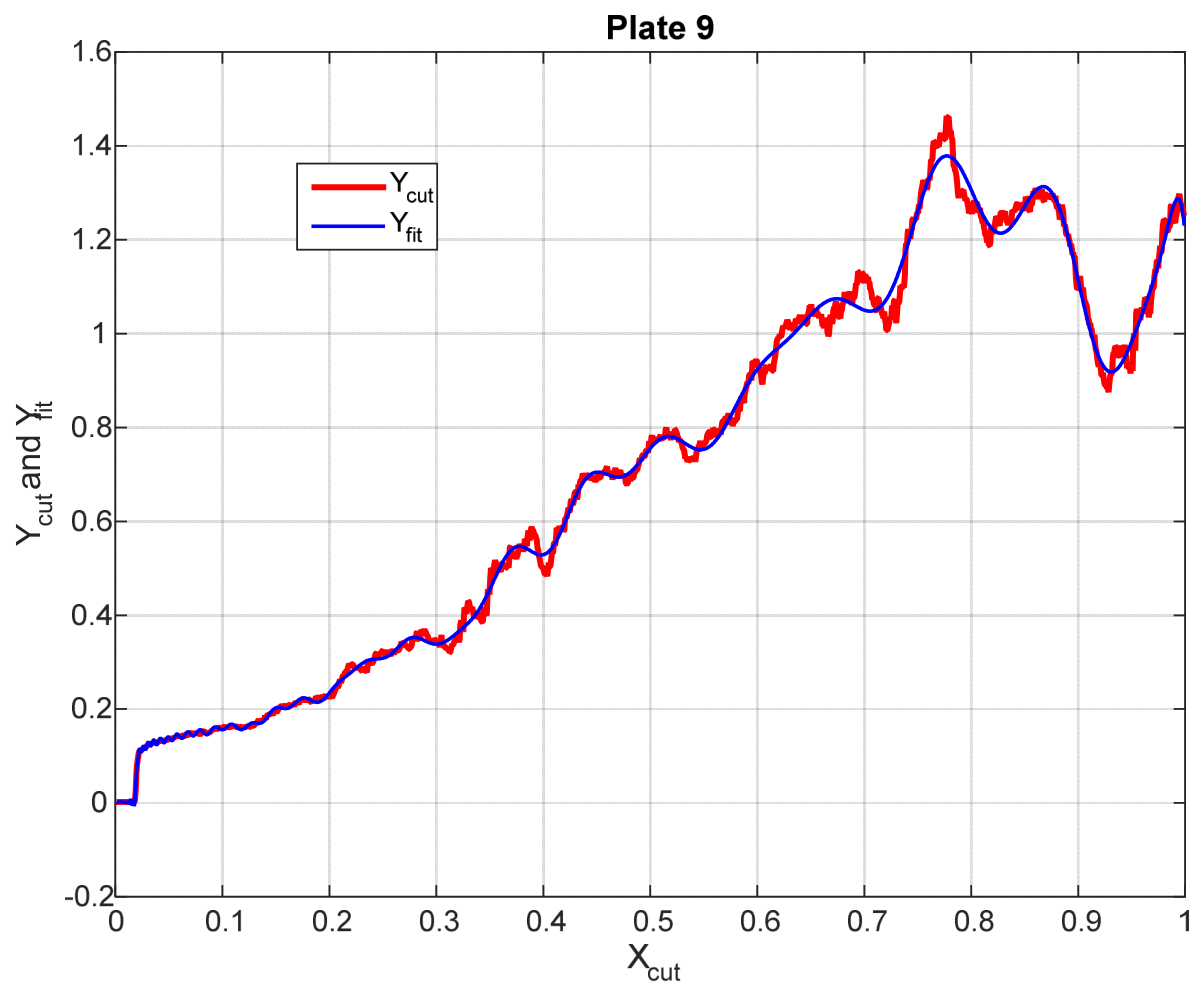
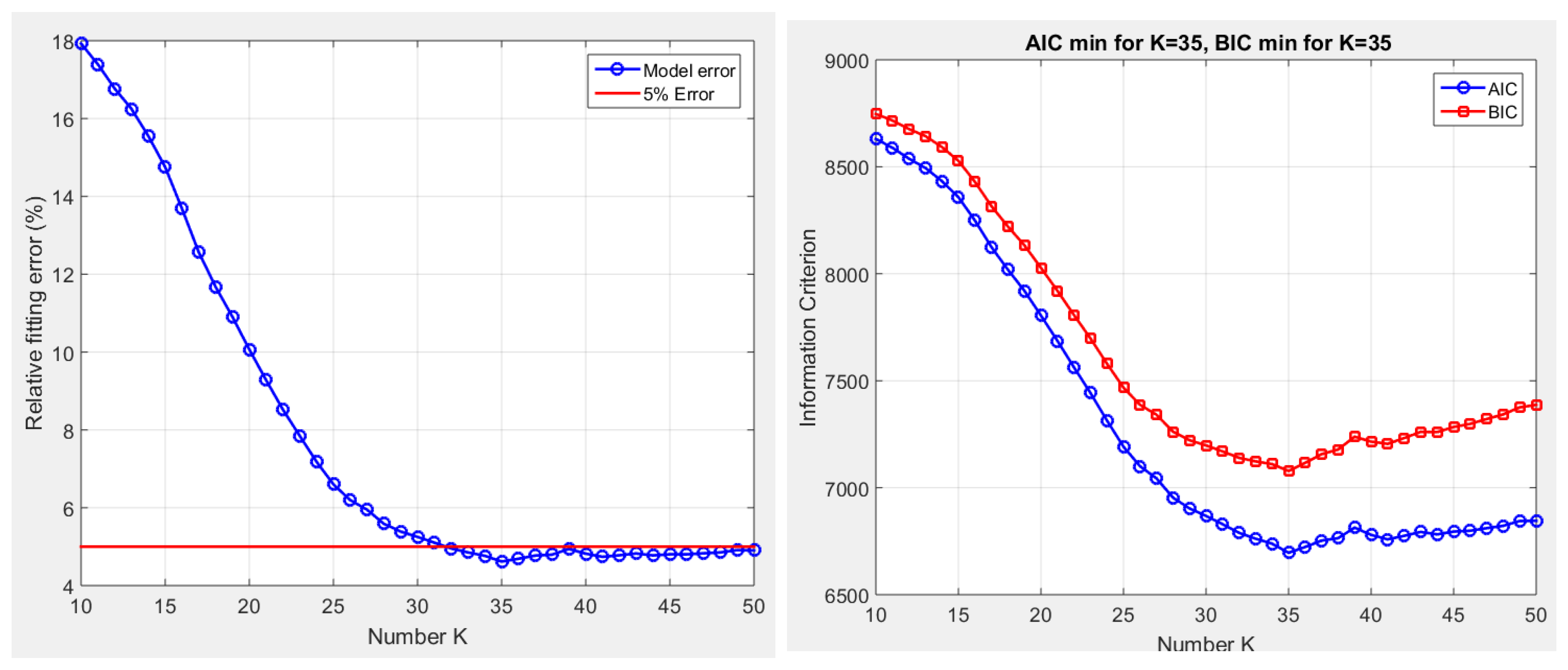
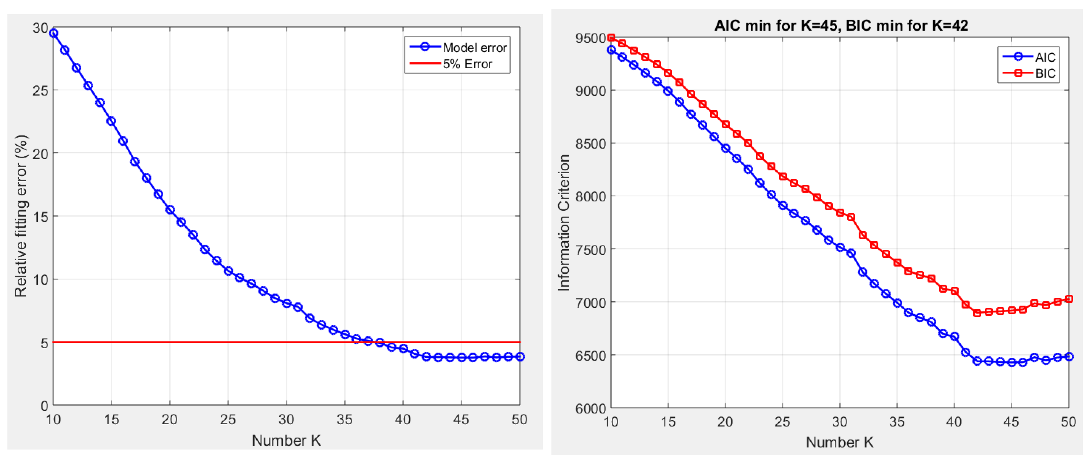
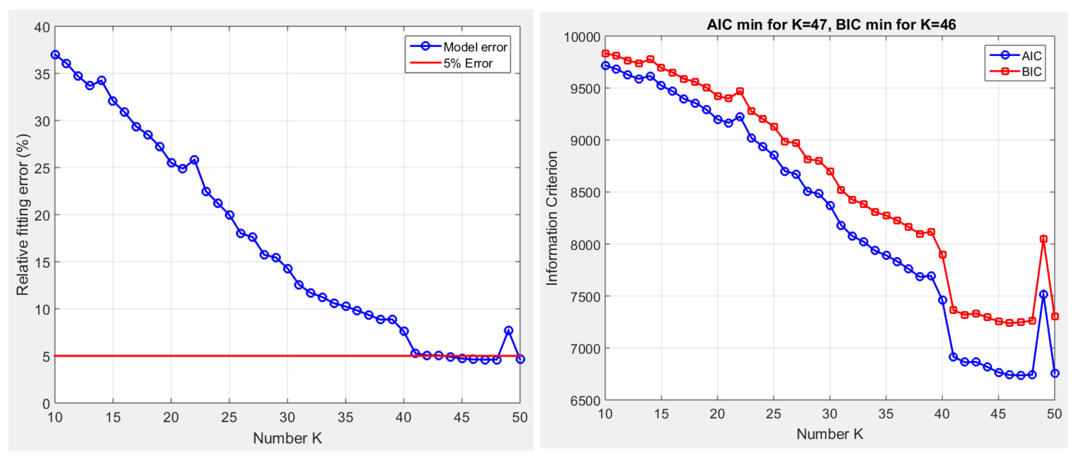
As shown on Figure 4a (see also Appendix A), the minimal value of the fitting error is achieved with K = 34 and ln(ξ) = 6.72, which corresponds to min(Error) = 4.98%. The comparison of the fitting function Y_fit(x) with the compressed data Y_cut (x) is shown in Figure 4b. For the other boards, fitting errors as a function of $K$ are presented in Appendix A. 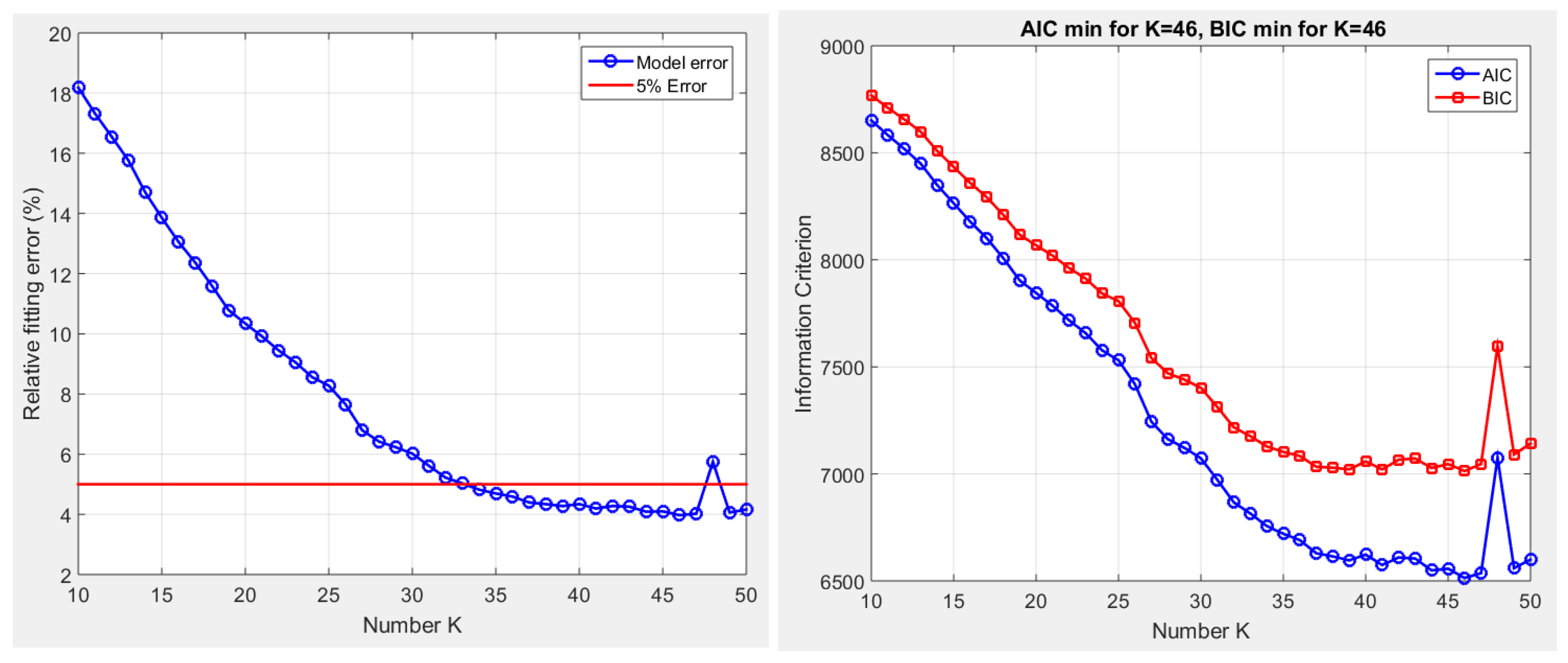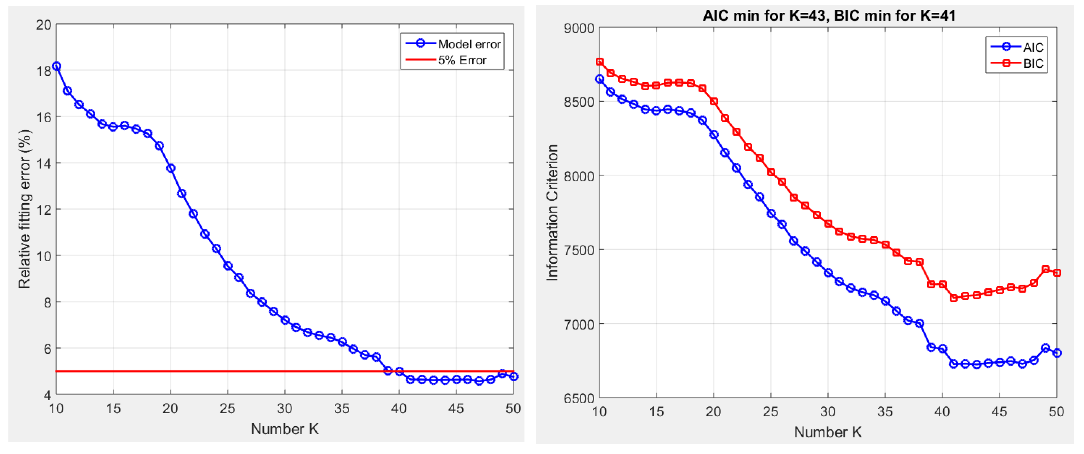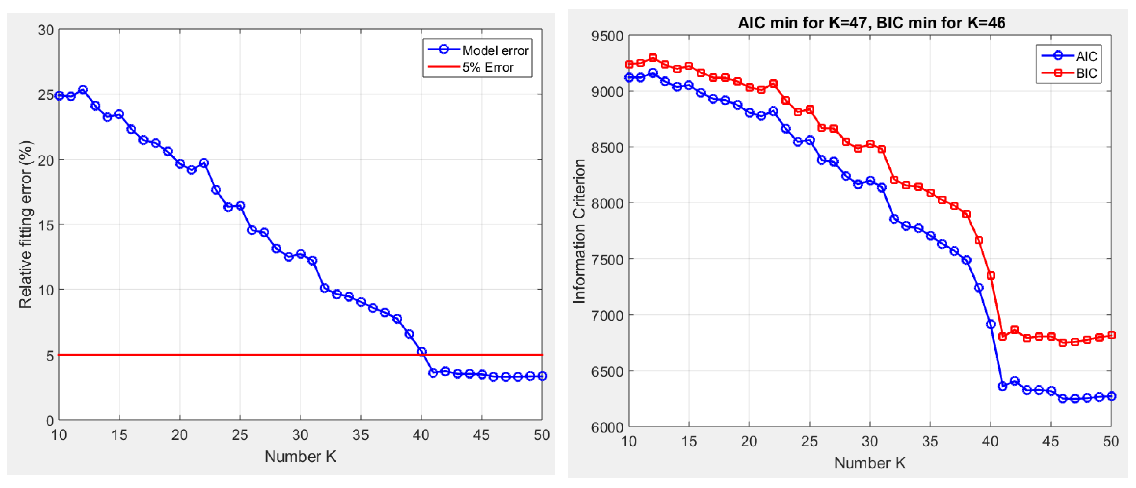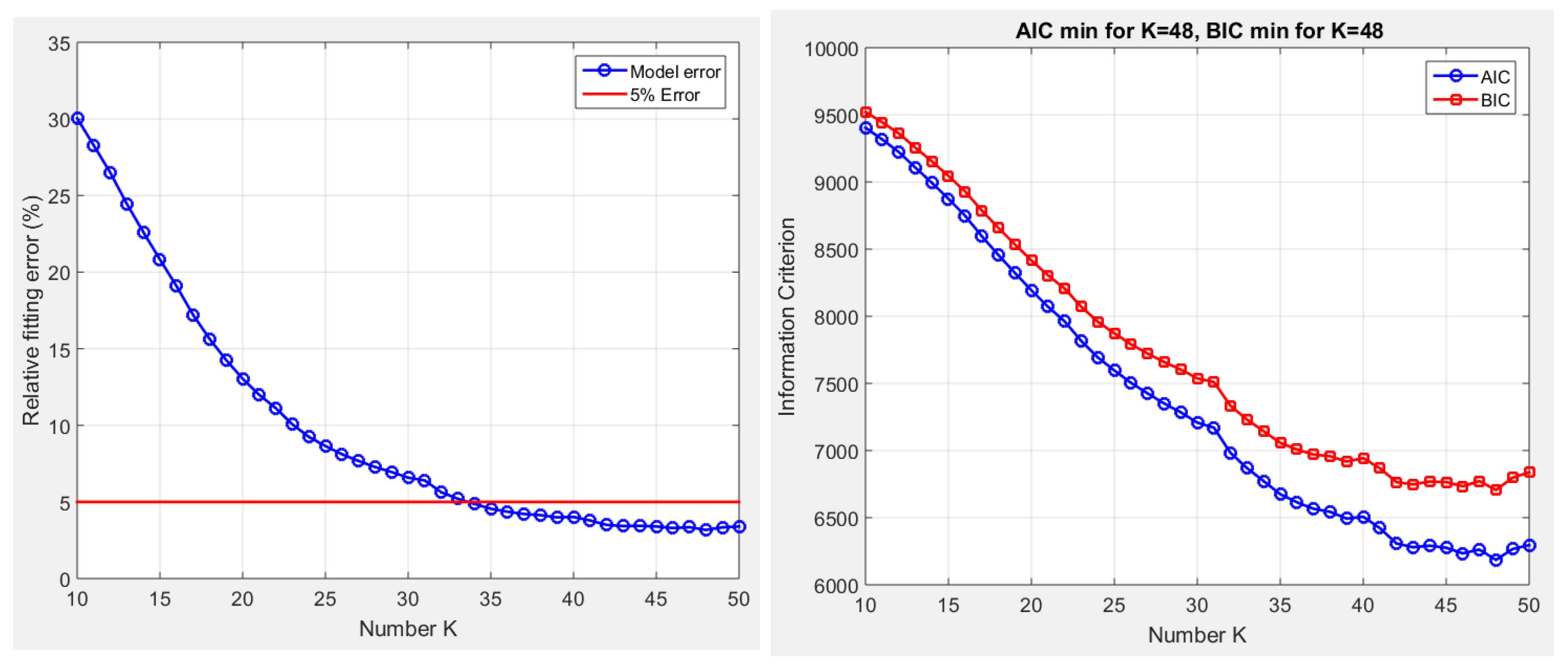To select the optimal number of modes $K$ and to prevent overfitting, the relative error criterion (Err < 5%) was supplemented with the Akaike Information Criterion (AIC) and the Bayesian Information Criterion (BIC). For a model with $p=2K+2$ parameters and a mean square error MSE (mean squared difference between the values predicted by the model and the observed values), these criteria are defined as:

$$AIC=Nln\left(MSE\right)+2p$$

$$BIC=Nln\left(MSE\right)+p ln\left(N\right)$$

where $N$ is the number of data points. The AIC balances goodness of fit against model complexity with a constant penalty per parameter, while the BIC imposes a stronger penalty that grows with N.

Both criteria were computed for $K$ ranging from 10 to 50 for each board. In all cases, we found that the AIC and BIC minima occurred at $K$ values slightly larger than those required to reach the 5% relative error (relation (6)) threshold. This indicates that the empirical 5% criterion is more conservative than the statistical criteria, and a simpler model than what AIC or BIC would suggest was thus chosen. This conservative choice is deliberate, the objective being to capture the dominant scaling features of the discharge signals with a parsimonious model, not to fit every fluctuation.

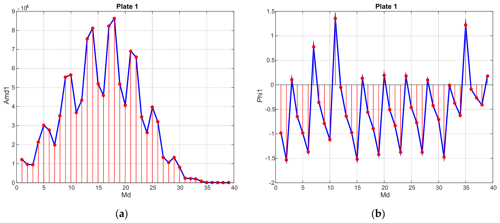
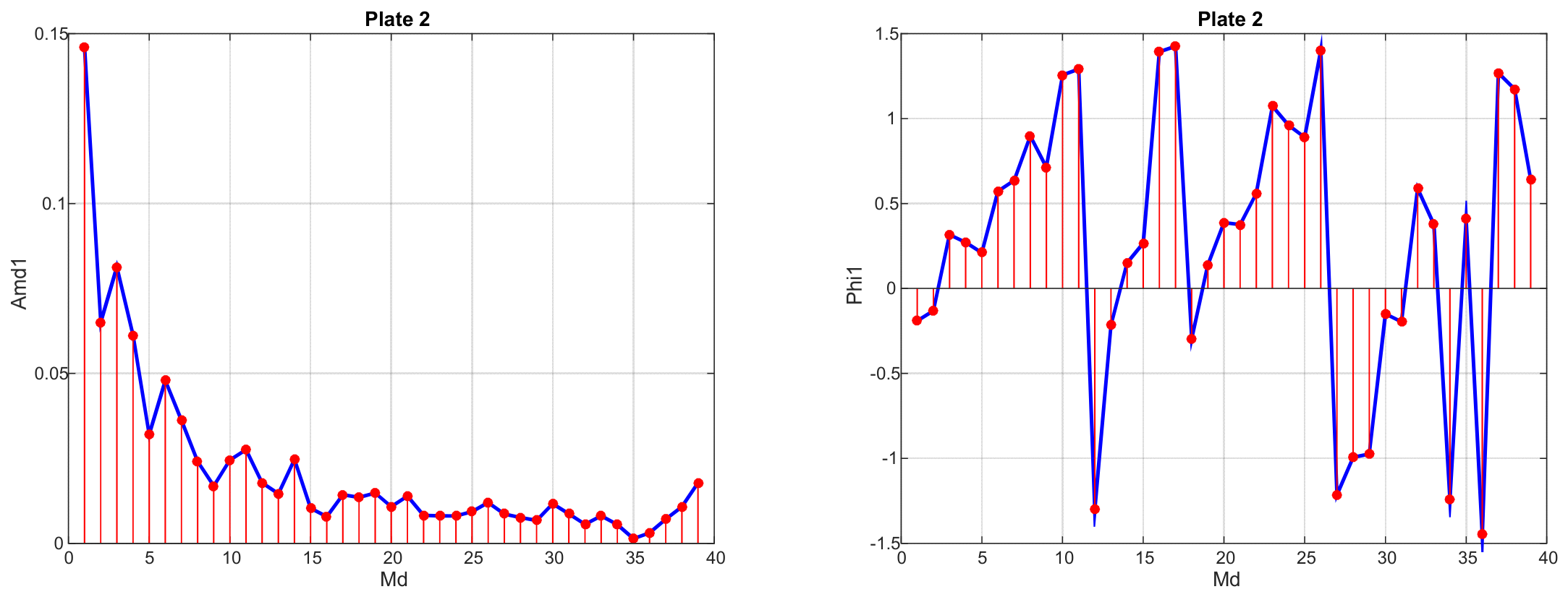
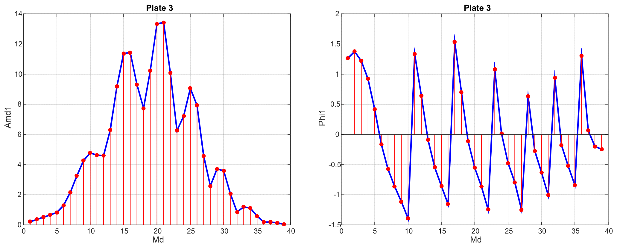
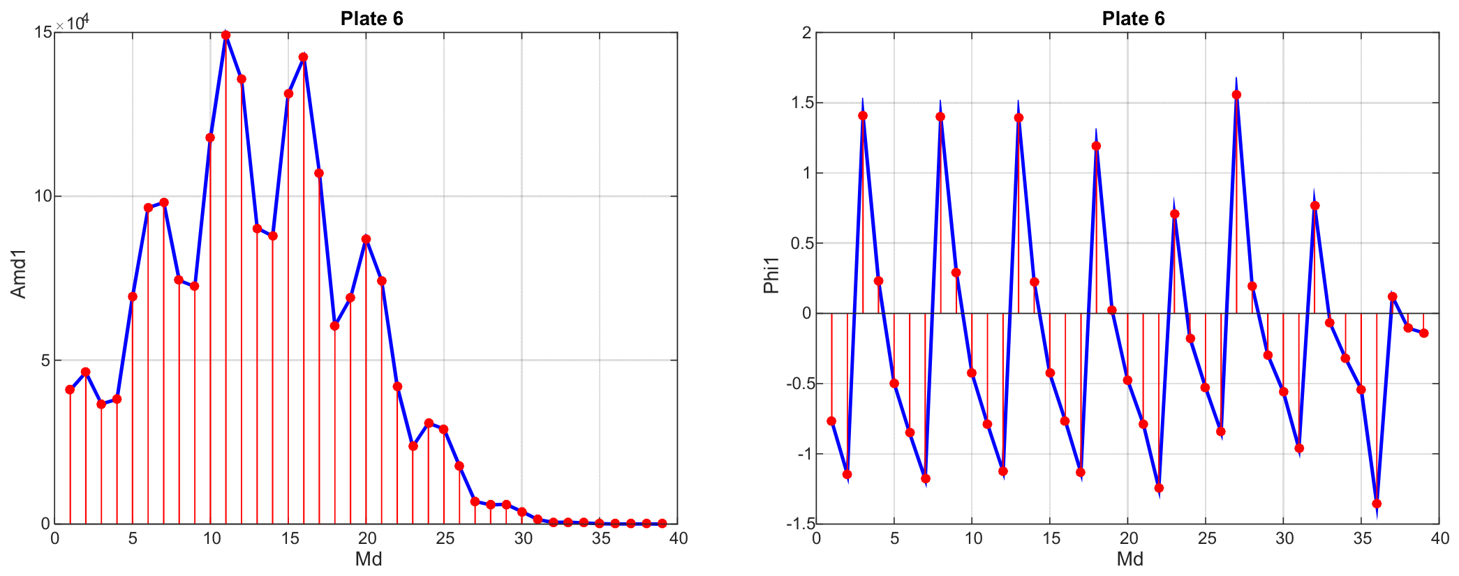
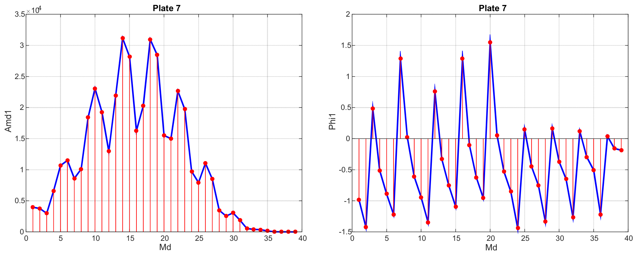
These parameters help to find the final fit with the help of expression (5) because the unknown set of amplitudes A₁, Ac_k⁽¹⁾ and As_k⁽¹⁾ are found by the linear least square method. Figure 5 shows the modulus distribution of the amplitudes $Am{d}_k=\sqrt{{\left(A{c_k}^{\left(1\right)}\right)}^2+{\left(A{s_k}^{\left(1\right)}\right)}^2}$ and phases $P{h}_k={\mathit{tan}}^{-1}\left({\displaystyle \frac{A{s}_k^{\left(1\right)}}{A{c}_k^{\left(1\right)}}}\right)$.

To assess the quality of the fit, the residual $\epsilon \left(x\right)=Y_{cut}\left(x\right)-Y_{fit}\left(x\right)$ was analyzed. For board 1, the residual statistics are: mean = 1.52 × 10⁻⁸ (effectively zero), standard deviation = 2.56 × 10⁻², skewness = −0.3496, and kurtosis = 4.6463. The excess kurtosis (≈1.65) indicates heavier tails than a normal distribution, consistent with the intermittent nature of the discharge process. The Ljung–Box test for 20 lags yields Q = 7329.67 (p < 10⁻⁴), confirming significant residual autocorrelation at short lags. Similar results were obtained for the other boards.

These findings indicate that the two-exponent fractal elements model captures the dominant scaling features but leaves residual correlations, likely due to higher-order memory effects, non-stationarities, or the stochasticity of percolation pathways. The model should therefore be interpreted as an effective phenomenological description rather than an exact physical representation.

The two figures in Figure 5a,b form the desired amplitude-frequency response for the current J₁ (in board 1). Other sets of currents produced by boards 1 to 9, denoted J₁ to J₉, can be treated in the same manner. The basic fitting parameters are given in

Table 2. Fitting parameters obtained.

Board Number	lnξ	A1	Fitting Error (%)	Re (λ1)	Re (λ2)	ν1	ν2
1	6.7191	−9234.67	4.9832	1.48195	1.48195	−1.29327	0.24139
2	4.6604	0.933775	4.61792	0.66565	2.55315	−1.03556	−0.08732
3	6.0053	−0.941752	4.48549	1.53612	0.156581	−1.39542	0.07147
4	6.6699	963,846	4.60583	3.0499	3.0499	−0.539923	0.19021
5	6.6691	−1646.89	3.31462	0.53328	−0.49091	1.68137	−0.09426
6	6.6691	−10,035.2	4.39871	1.74121	0.67771	−0.987662	0.08315
7	6.5049	−1378	3.75676	0.56439	1.87465	−1.08315	−0.08793
8	7.3094	−126,749	4.59444	0.75595	0.665377	1.26316	−0.03827
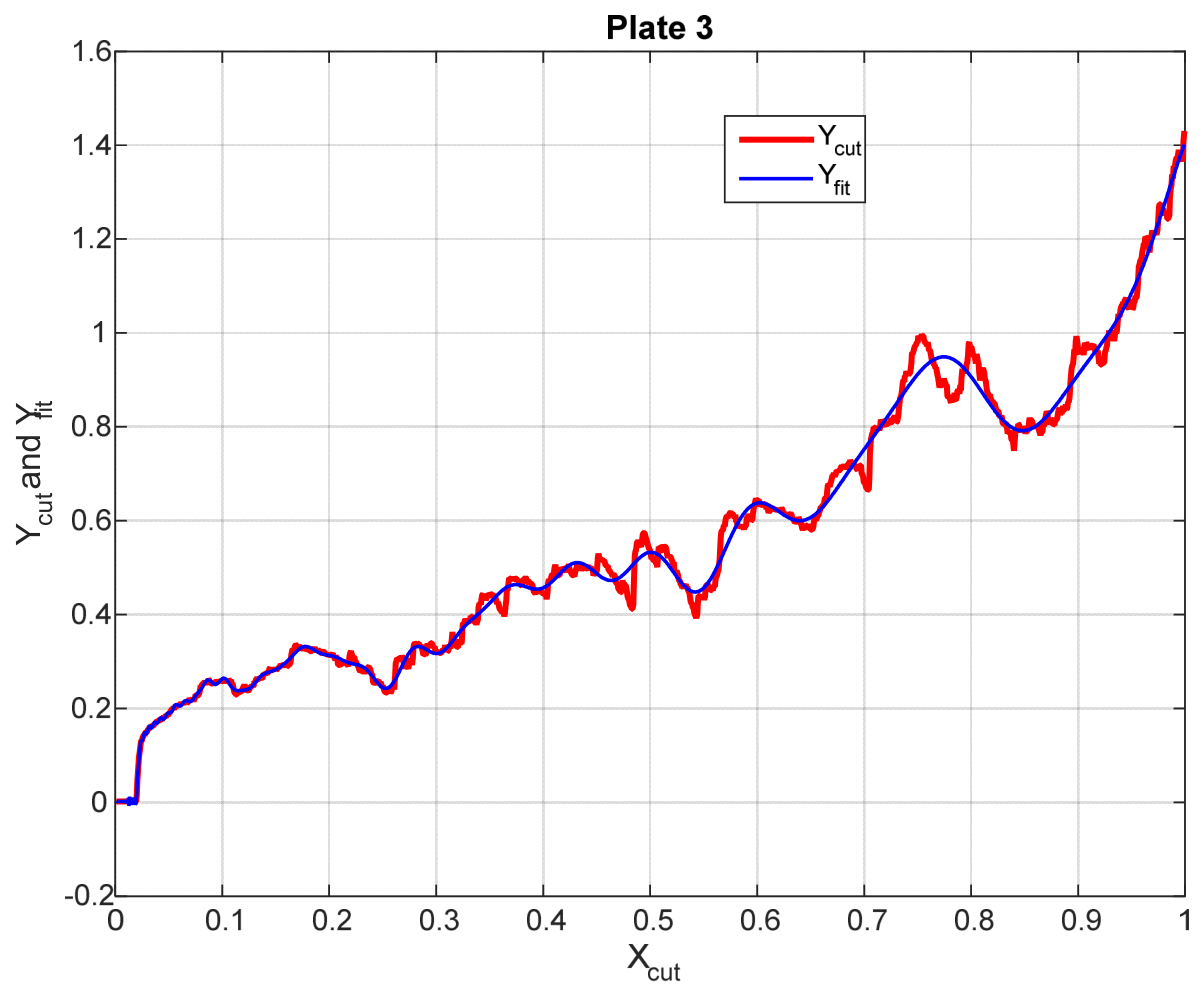
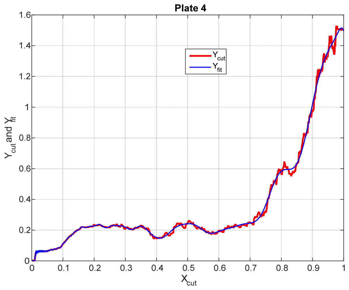
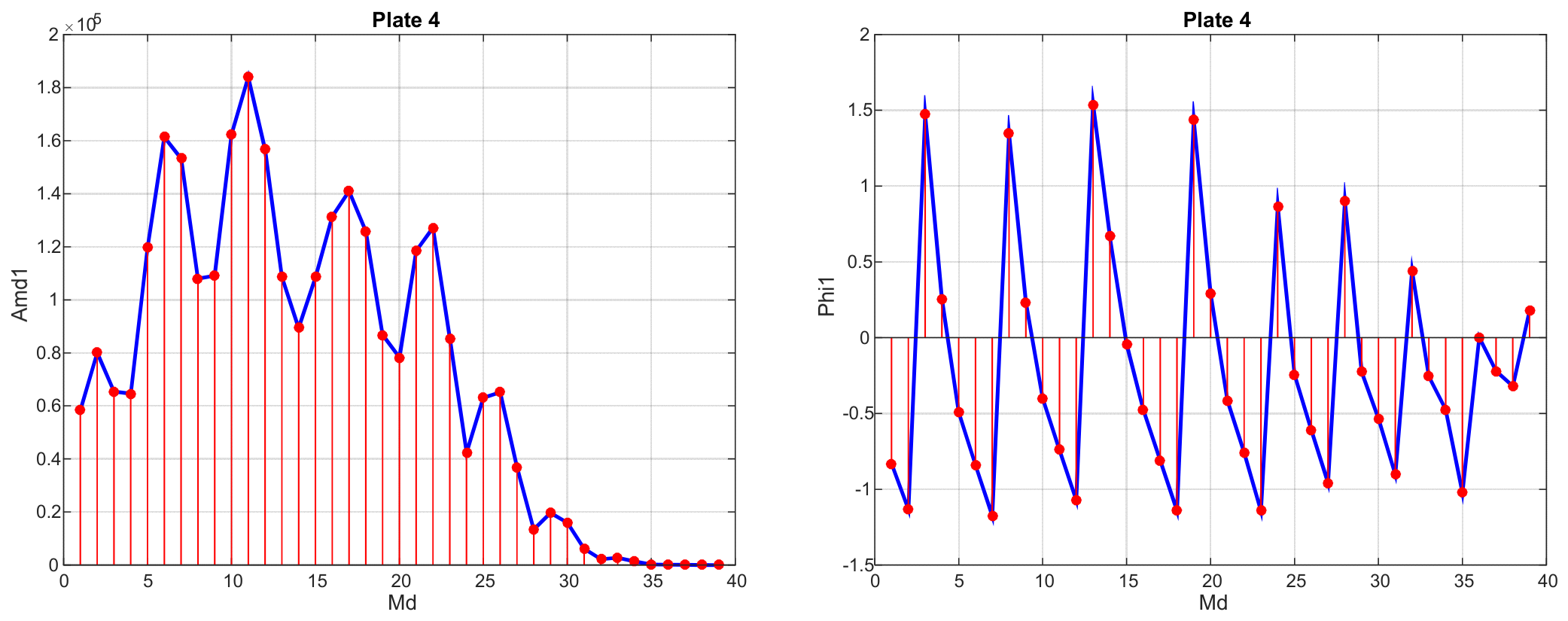
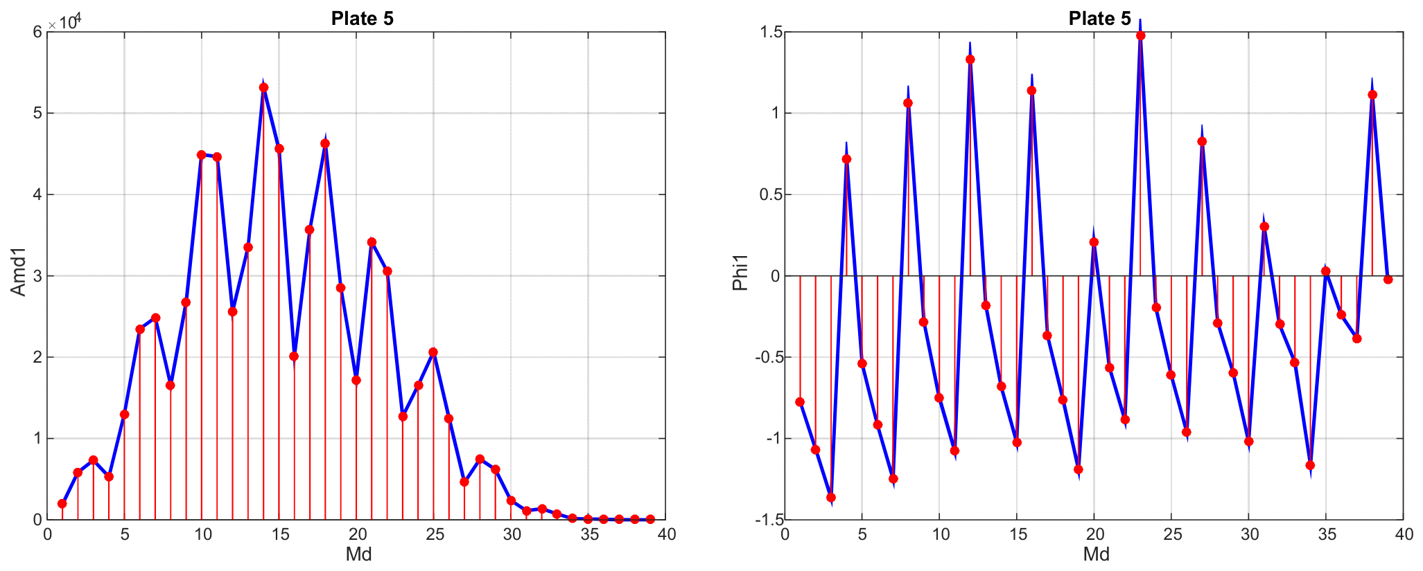
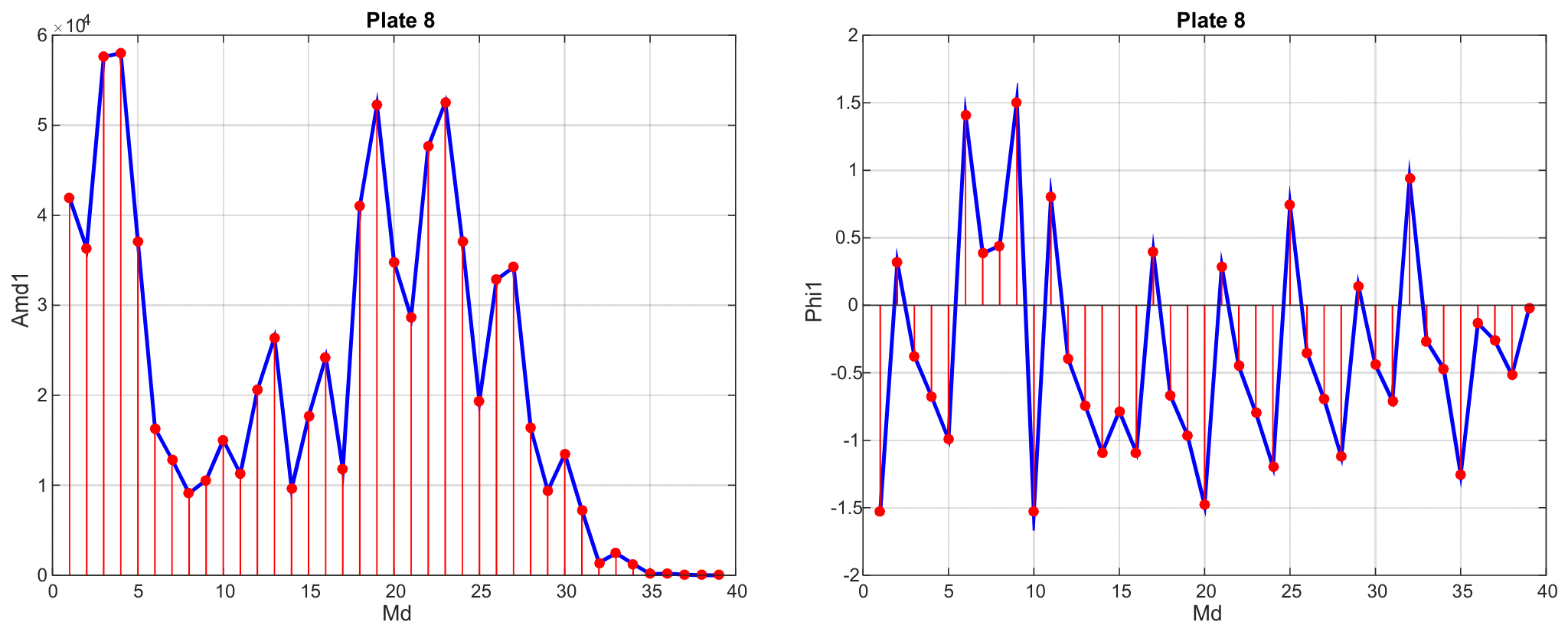
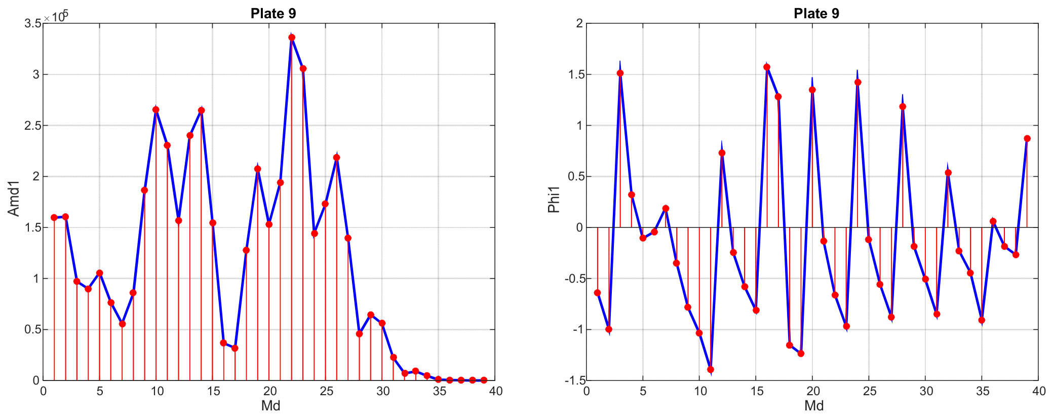
9	6.832	96,472.2	3.17416	0.46112	2.05906	−0.824375	−0.11330

, and the figures for boards 2 to 9 are available in Appendix A.

The set of the basic fitting parameters that correspond to the quantitative description of the currents (J₁–J₉) was realized with the help of the contacts depicted in Table 1.

To establish the macroscopic robustness of the fractal mode decomposition from the Nigmatullin–Chen theory and to ensure that the extracted exponents and amplitudes do not result from overfitting, a descriptive statistical validation procedure was implemented. The global fitting model (relation (5)) exhibits a hybrid mathematical structure: the structural scaling parameter $ln\left(\xi \right)$ and the number of modes $K$ act as highly nonlinear variables determined by minimizing the global relative error, while the associated set of amplitudes ($A_1$, $A_{ck}$, $A_{sk}$) is solved deterministically via the linear least squares method. In order to precisely quantify the joint stochastic uncertainty of these two sets of parameters, the global asymptotic covariance matrix ${\mathsf{\Sigma }}_{\theta }$ was evaluated at convergence from the numerical Jacobian matrix $J$ of the complete model, such that:

$${\mathsf{\Sigma }}_{\theta }=s^2{\left(J^{T}J\right)}^{-1}$$

(7)

where

$$s^2={\displaystyle \frac{1}{N-p}}{\displaystyle {\sum }_{i=1}^N}{\left(Y_i-\widehat{Y_i}\right)}^2$$

(8)

is the unbiased residual variance of the model, $N$ being the number of points in the compressed current signal ($N$ = 2000) and $p$ the total number of free parameters ($p=2K+2$). The standard error ($SE$) of each parameter ${\theta }_i$ corresponds to the square root of the associated diagonal element:

$$SE\left({\theta }_i\right)=\sqrt{{\left({\mathsf{\Sigma }}_{\theta }\right)}_{ii}}$$

(9)

The individual 95% confidence intervals are then defined by:

$${\theta }_i\pm t_{{\displaystyle \frac{1-0.95}{2}},N-p} SE\left({\theta }_i\right)$$

(10)

Given the large number of degrees of freedom ($N-p\approx 1948$), Student’s t-distribution converges strictly to a standard normal distribution ($t_{0.025}\approx 1.96$). Applying this method to board 1 provides the confidence intervals and the p values for the first parameters and confirms the very high selectivity of the model. The confidence interval obtained for the scale parameter is extremely narrow ($ln\left(\xi \right)=6.719\pm 0.027$), statistically validating the hypothesis of stable structural scale invariance within the disordered medium. Furthermore, the calculated p-values for the lower rank harmonics ($k\le 10$) are less than 10⁻⁴ which demonstrates that these fractal spectral modes carry highly significant physical information and are clearly distinct from residual measurement noise. It must be noted that multiple comparisons were performed across the K = 34 harmonic amplitudes and that a Bonferroni correction would not change the qualitative conclusions (the p-values remain well below 0.05/K).

Given the burst-like nature of the current signals, the assumption of residual independence underlying the covariance-matrix formula may not hold exactly. To address this, confidence intervals were also estimated using a moving block bootstrap procedure [16,17,18] with block length L = 50 samples (chosen based on the decay time of the residual autocorrelation function). The block-bootstrap confidence intervals are slightly wider than the asymptotic ones but remain consistent with the reported parameter values, confirming that the parameter estimates are robust to residual autocorrelation. The results reported in

Table 3. Statistical analysis of obtained parameters.

Parameter	Estimation	Standard Error	95% Confidence Interval	p-Value
$A_1$	−9234.67	9.13 × 102	[−9.80 × 103, −9.61 × 103]	2.50 × 10−3
$A_{c1}$	−2.27 × 103	2.16 × 102	[−2.70 × 103, −1.85 × 103]	<10−4
$A_{s1}$	3.72 × 103	3.55 × 102	[3.03 × 103, 4.42 × 103]	<10−4
$A_{c2}$	−7.85 × 103	7.46 × 102	[−9.31 × 103, −6.38 × 103]	<10−4
$A_{s2}$	4.00 × 103	3.82 × 102	[3.25 × 103, 4.75 × 103]	<10−4
$A_{c3}$	−1.34 × 104	1.27 × 103	[−1.58 × 104, −1.09 × 104]	<10−4
$A_{s3}$	−1.14 × 103	1.06 × 102	[−1.35 × 103, −9.32 × 102]	<10−4

are the asymptotic intervals.

4. Results and Discussion

4.1. High-Voltage Discharge in Wood as a Physical System

Wood is a highly disordered medium whose electrical response depends on fibrous structures, pores, and moisture content. The discharge process is intrinsically non-linear [19]: the Joule effect induces irreversible carbonization that locally alters conductivity and concentrates the electric field, which rules out any description by classical exponential relaxation.

4.2. Self-Similarity and Scale Invariance of the Current Signals

The measured current signals are highly fluctuating but exhibit clear statistical self-similarity under temporal compression factors of 10 to 100, proving the absence of a characteristic time scale [20]. The successful decomposition into fractal modes confirms that these fluctuations are intrinsic to the physical process and do not constitute experimental noise.

4.3. Interpretation of the Scaling Parameter Ln(ξ)

The parameter ln(ξ) proves to be remarkably stable across all configurations and electrode arrangements. Within the framework of percolation theory [21], it is interpreted as the characteristic scale ratio governing the hierarchical activation of conducting pathways [22,23]. Its robustness indicates that this hierarchy is dictated by the internal microscopic heterogeneity of the wood rather than by the macroscopic geometry imposed on the surface.

4.4. Variability of Power-Law Exponents and Transport Pathways

Conversely, the exponents ν₁ and ν₂ vary significantly from one experiment to another. This dispersion reflects the sensitivity of the kinetics to the specific percolation pathways activated by the different aperture patterns and electrode configurations [24]. The discharge resembles a non-stationary percolation process where the exponents characterize the temporal organization of current peaks within a network with evolving connectivity.

4.5. Decoupling Between Geometric Fractality and Fractional Kinetics

Since the fractal dimension D_f of the carbonized patterns was not directly measured, no formal statistical correlation (such as Pearson’s coefficient) can be calculated between D_f and ν₁ and ν₂ (Table 2). Moreover, assigning a constant nominal value from the literature D_f approx 1.7 for these bush-like structures [9,25] would eliminate variance, making any correlation metric mathematically undefined. Fundamentally, there is a physical decoupling: D_f describes a static, temporally integrated geometric object, whereas ν₁ and ν₂ encode the non-stationary temporal dynamics of channel activation, influenced by the Joule effect and local moisture gradients. The exponents must therefore be viewed as effective descriptors of these evolving dynamics, independent of the final geometry or average macroscopic metrics.

4.6. Physical Implications and Outlook

These results confirm the effectiveness of the theory of fractal elements for extracting relevant physical parameters from highly irregular signals. The coexistence of a stable hierarchical scale (ln(ξ)) and variable transport exponents opens the way to comparative studies of dielectric breakdown in other heterogeneous media.

4.7. Reproducibility Across Identical Geometries

To assess the reproducibility of the fitting parameters, we compared boards with identical aperture patterns and electrode configurations: group A (boards 1, 2, 5), group B (boards 3, 6), group C (boards 4, 7), and group D (boards 8, 9). Within each group, the scale parameter ln(ξ) showed remarkable consistency, with relative variations below 2%. The kinetic exponents ν₁ and ν₂ exhibited larger variations (typically 5–15%), reflecting the stochastic nature of the discharge process and the sensitivity of the transport dynamics to sample-specific factors such as local moisture gradients and carbonization pathways. This reproducibility analysis confirms that the fractal elements decomposition yields stable and physically meaningful parameters, with ln(ξ) emerging as a robust characteristic of the wood–carbon system.

5. Conclusions

In this work, we investigated high-voltage surface discharges on wood as a prototype of transport and breakdown in a strongly disordered, evolving medium. The formation of Lichtenberg figures reflects the emergence of complex conductive networks governed by material heterogeneity, anisotropy, and irreversible structural transformations induced by Joule heating and carbonization.

The main experimental result of this study is the clear demonstration of self-similarity and scale invariance in the electrical current signals associated with the discharge process. The current fluctuations remain statistically invariant under temporal rescaling over more than one decade, indicating the absence of a characteristic time scale. This property justifies the application of the general theory of fractal elements and supports the interpretation of the measured signals as structured, self-similar objects rather than as noisy realizations of a smooth underlying trend.

Using the fractal elements framework, the current signals were successfully decomposed into a finite set of elementary self-similar modes characterized by scaling parameters and amplitudes. The stability of the global scaling parameter ln(ξ) across different geometries suggests the existence of a robust hierarchical organization of the discharge dynamics, likely controlled by intrinsic properties of the disordered wood–carbon system. At the same time, the variability of the extracted power-law exponents reflects the sensitivity of transport processes to the specific realization of percolation pathways activated during breakdown. It is important to emphasize that the excellent fitting performance of the fractal elements model (errors below 5%) does not, by itself, constitute a physical validation of the model. As with any flexible phenomenological model, good fit quality indicates that the model captures the essential features of the data, but it does not guarantee that the fitted modes are unique or that they correspond to fundamental physical processes. The physical interpretation of the parameters presented here is supported by their correlations with macroscopic discharge features and by their reproducibility across identical geometries. However, establishing a rigorous first-principles connection between the fractal elements decomposition and the underlying physics of dielectric breakdown will require further theoretical and experimental investigation.

Importantly, the present results do not establish a direct correspondence between the fractal geometry of the Lichtenberg figures and a well-defined fractional order governing current kinetics. Rather, they demonstrate that self-similarity in time emerges naturally from the collective dynamics of an evolving percolation network, in which memory effects and nonlocal interactions arise from irreversible material modifications. In this context, self-similarity should be regarded as a necessary precursor to fractional kinetics, but not as a sufficient condition.

While the fractal elements decomposition yields a good first-order approximation of the current signals (relative fitting error < 5%), residual analysis reveals persistent autocorrelations and non-Gaussianity. This indicates that the discharge dynamics may involve higher-order memory effects that are not captured by the two-exponent model. Future work could explore extensions with additional exponents or non-stationary frameworks to account for these residual structures.

This work therefore represents a first step toward a statistical-physics description of electrical breakdown in heterogeneous dielectrics based on scale invariance and disorder-controlled transport. Future investigations combining longer time series, complementary statistical diagnostics (such as waiting-time and correlation analyses), and controlled modifications of the medium will be required to determine whether the observed self-similarity ultimately corresponds to genuine fractional kinetic equations or to a broader class of scale-free, nonstationary transport processes.