Longitudinal Flow Dynamics and Stress Relaxation of a Fractional-Order Rheological Maxwell Fluid in Pipes of Variable Cross-Section

Abstract

The manuscript contains the new scientific results of theoretical modeling of longitudinal flow dynamics (creeping) of a viscoelastic fluid governed by a fractional-type rheological Maxwell model material within a pipe of variable cross-section. Structurally, the paper utilizes a fractional-order differential operator defined on the interval 0 < α ≤ 1 to form a differential constitutive relationship between normal stress and axial dilatation, which is subsequently combined with D’Alembert’s dynamic equilibrium principles to form a governing fractional-order partial differential equation (PDE). Then the Bernoulli method of particular integrals for the separation of variables is applied to decompose the continuous field model into spatial eigen-amplitude ordinary differential equations (ODEs) and temporal fractional-order evolutionary ODEs, which are then solved analytically using series expansions of Laplace transforms and inverse Laplace transforms to yield three-dimensional parametric surfaces representing normal stress relaxation. The scientific findings indicate that normal stress asymptotically relaxes to zero under constant axial dilatation over time, showing a highly nonlinear dependence on the fractional order α.

1. Introduction

The content of this article and the new scientific results presented in it were inspired by the author’s own knowledge, accumulated over years of teaching students at the university, as well as work and research in various fields of science and industry. In this sense, and also due to the lack of published literature in the field of rheological dynamics of Maxwellian fractional-type viscoelastic flow models, this introductory part also lists the author’s own references, conceptually connected with the author’s latest published References from the last three years, 2023–2025.

The author learned his first scientific knowledge of the longitudinal and transverse dynamics of deformable, ideally elastic media from Professor Dr. and Mathematician Danilo P. Rašković through exceptional lectures and his excellent university monographs (see References [1,2,3,4]). In particular, the author emphasizes the analogies he spoke about and emphasized the analogous dynamics, which are described by the same mathematical descriptions, and among them the analogies of the dynamics of torsional and longitudinal oscillations of rods (see the basic original and previously published References [5,6,7], of Mihail Petrović, the founder of the Serbian school of mathematics, who completed his studies as the most successful student of generation of mathematics and physics at the University of the Sorbonne and was one of the three doctoral students of Julius Henri Poincaré.

At the invitation of one of the editors, Bilen Emek Abali, the author of this paper wrote and published in 2020 [8] on Forced Longitudinal Fractional-Type Vibrations of a Rod with Variable Cross-Section in the Springer Nature book Developments and Novel Approaches in Nonlinear Solid Body Mechanics.

Four years later, in 2024, the author of this paper, driven by strong scientific inspiration, returned to research in the field of applications of fractional calculus in mechanics, with a sudden and spontaneous scientific inspiration, based on previously acquired knowledge of classical rheological models and carrying in his mind the ideas of applying fractional calculus, and in a very short time achieved new scientific results, which he formulated in References [9,10], published in a specialized journal called ‘’Fractal and Fractional’’, and with the exceptional support of the Journal’s Editorial Board and especially one of the associate editors. This series of new papers also includes the published Reference [11].

In the published References [8,9], new scientific results from theoretical–analytical research on the dynamics of fractional-type rheological models for elastoviscous materials in a rod of variable cross-section are presented. This is a fractional-type material with properties of subsequent elasticity (post-elasticity). The material is a rheological fractional-type Kelvin–Voigt model with properties of elastoviscosity and subsequent elasticity (post-elasticity), as described in detail in Reference [12]. These properties lead to the appearance of rheological longitudinal fractional-type oscillations in the rod. We described this motion solely by a fractional-order partial differential equation and determined its approximate analytical solutions and corresponding expressions for describing the eigen and forced rheological modes of the fractional elastoviscous rheological type. We considered different boundary conditions and different cross-sections of a rod of variable cross-section. We derived an ordinary differential equation of fractional order in terms of time functions for each amplitude form of oscillation and obtained approximate analytical solutions, along with approximate analytical expressions for the eigen and forced modes. We determined the amplitude functions. We graphically displayed the surfaces of the eigen and forced modes as functions of the differentiation exponent for the fractional-order and time-dependent cases. References [8,9] contain differential equations for the amplitude functions of longitudinal rheological oscillations of an ideally elastic rod, as well as tables of eigenvalues for different cross-sections and boundary conditions. Detailed descriptions of the amplitude functions for longitudinal oscillations of a rod of ideally elastic material, for different cross-sections and different boundary conditions, are also given.

In this paper, unlike the previous one, we will present new scientific results of studying the flow (creep) dynamics of the rheological Maxwell model of fractional-type material’s viscoelastic fluids with the material’s normal stress relaxation property in a pipe of variable cross-section. These properties lead to the appearance of longitudinal flows (creeping) in the rheological Maxwell model of fractional-type material. We described this flow (creeping) motion only by a partial differential equation of fractional order in terms of normal stresses and determined its approximate analytical solutions and the corresponding approximate analytical expressions for the eigen and forced modes of the normal stress flow (creeping) in terms of the eigen-time functions for the corresponding eigen-amplitude modes. We considered different possible boundary conditions for the normal yield (creeping) stresses in the rheological Maxwell model of fractional-type materials for pipes of variable cross-section.

In the research and scientific results presented in the previously published articles that we cited, as well as in the new ones that we present in this paper, we used knowledge from fractional calculus. Therefore, we will point out here a number of characteristic references from fractional calculus. Reference [11] approaches the application of fractional calculus to the study of natural and forced rheological oscillations of rods made of elastic-viscous fractional-type material with constant or variable cross-section. We point out that these references, using an approximate analytical approach, determined inverse Laplace transforms for determining natural and forced modes of time functions in the corresponding natural amplitude functions for certain cross-sections of the rod and certain boundary conditions.

Generalized Fractional Calculus and Applications, as well as Theory and Applications of Fractional Differential Equations, are presented in References [12,13,14]. These References are useful for studying the theory of fractional calculus. The following Reference [15] focuses on Models and Numerical Methods for applications in Fractional Calculus.

The author of this paper especially emphasizes the following Reference [16], which is related to Fractional Calculus in the form of An Introduction For Physicists, and is also useful for researchers from various fields of science.

To introduce the reader to the structure of the article, we list the chapters that the article contains as follows:

2.

Constitutive differential relation of the fractional order of the Maxwell model

3.

Partial differential equation of flow dynamics, fractional order

4.

Decomposition of the partial differential equation of longitudinal flow dynamics of the Maxwell model of a material

5.

Eigen-amplitude functions for the realization of flow dynamics

6.

Differential equations of fractional order in terms of eigen-time functions

7.

Graphical representation of eigen-time functions

8.

Discussion

9.

Conclusions

References

2. Constitutive Differential Relation of the Fractional Order of the Maxwell Model

In the Maxwell model of fractional-type material, the following rheological elements are sequentially related as follows:

* The ideally elastic solid Hooke element of the constitutive relation between the normal stress ${\sigma }_z\left(t\right)$ and axial dilatation ${\epsilon }_z\left(t\right)$, in a state of axial strain, has the following form:

$${\sigma }_z=E{\epsilon }_z$$

(1)

* An ideally viscous fluid generalized fractional-type Newtonian element constitutive differential relations of fractional order of normal stress ${\sigma }_z\left(t\right)$ and ${\mathrm{D}}_t^{\alpha }\left[{\epsilon }_z\right]$ fractional type of axial dilatation ${\epsilon }_z\left(t\right)$, in the state of axial flow (creeping), is of the following form:

$${\sigma }_{z,\alpha }=E_{\alpha }{\mathrm{D}}_t^{\alpha }\left[{\epsilon }_z\right], 0<\alpha \le 1$$

(2)

where ${\mathrm{D}}_t^{\alpha }\left[•\right]$ is the fractional-order differential operator, the exponent of the fractional order of differentiation $\alpha$, on the interval $0<\alpha \le 1$.

In this paper, we will use the following differential operator of non-integer (fractional) order ${\mathrm{D}}_t^{\alpha }\left[•\right]$, which we define with the following derivative and integral:

$${\mathrm{D}}_t^{\alpha }\left[{\epsilon }_z\left(t\right)\right]={\displaystyle \frac{d^{\alpha }{\epsilon }_z\left(t\right)}{d{t}^{\alpha }}}={{\epsilon }_z}^{\left(\alpha \right)}\left(t\right)={\displaystyle \frac{1}{\Gamma \left(1-\alpha \right)}}{\displaystyle \frac{d}{dt}}{\displaystyle {\displaystyle \underset{0}{\overset{t}{\int }}}\frac{{\epsilon }_z\left(\tau \right)}{{\left(t-\tau \right)}^{\alpha }}}d\tau ,\hspace{1em}for\hspace{1em}0<\alpha \le 1$$

(3)

where $\Gamma \left(1-\alpha \right)$ is the special Gamma function, which is defined in integral form (see Reference [11]):

$$\Gamma \left(1-\alpha \right)={\displaystyle {\displaystyle \underset{0}{\overset{+\infty }{\int }}}{e}^{-t}}{t}^{-\alpha }dt,\hspace{1em}1-\alpha >0$$

(4)

This can also be defined in general form as a function of a variable $x$ as follows:

$$\begin{array}{ll}\Gamma (x)={\displaystyle {\int }_0^{+\infty }{e}^{-t}}{t}^{x-1}dt,\hfill & x>0\hfill \\ \Gamma (x+1)=x\Gamma (x),\hfill & x>0\hfill \end{array}$$

(5)

As the article concerns the rheological dynamics of the Maxwell model of fractional-type materials, we limit ourselves to applications of fractional calculus, without the intention of making mathematical contributions to the field. For details on fractional-order differential operators and other details, we refer the reader to References [9,10,11] from the attached list or to the wider mathematical literature.

The constitutive differential relation of the rheological Maxwell model of the fractional type of viscoelastic material is composed using the sum ${\mathrm{D}}_t^{\alpha }\left[{\epsilon }_z\right]$ of the fractional-type dilation velocities, ${\mathrm{D}}_t^{\alpha }\left[{\epsilon }_{z,1}\right]$ and ${\mathrm{D}}_t^{\alpha }\left[{\epsilon }_{z,2}\right]$, in the longitudinal direction ${\mathrm{D}}_t^{\alpha }\left[{\epsilon }_z\right]$ and ${\mathrm{D}}_t^{\alpha }\left[{\epsilon }_{z,2}\right]$, which is as follows:

$${\mathrm{D}}_t^{\alpha }\left[{\epsilon }_z\right]={\mathrm{D}}_t^{\alpha }\left[{\epsilon }_{z,1}\right]+{\mathrm{D}}_t^{\alpha }\left[{\epsilon }_{z,2}\right]$$

(6)

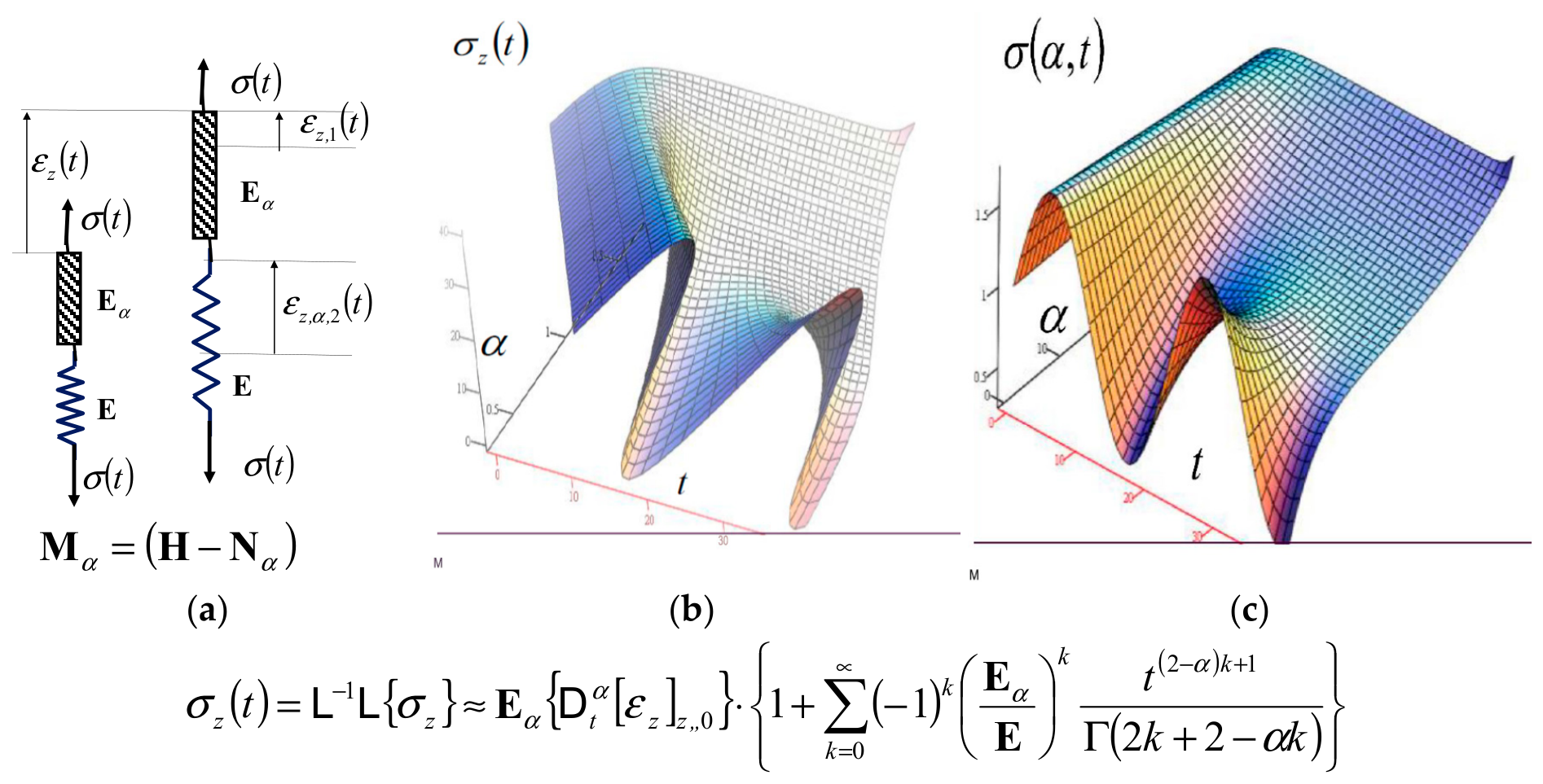
Accordingly, ${\epsilon }_{z,1}={\displaystyle \frac{{\sigma }_z}{E}}$ follows ${\mathrm{D}}_t^{\alpha }\left[{\epsilon }_{z,1}\right]={\displaystyle \frac{1}{E}}{\mathrm{D}}_t^{\alpha }\left[{\sigma }_z\right]$ and ${\mathrm{D}}_t^{\alpha }\left[{\epsilon }_{z,2}\right]={\displaystyle \frac{{\sigma }_z}{E_{\alpha }}}$. It follows that the expression is a sum axial dilatation analysis (see Figure 1a): ${\mathrm{D}}_t^{\alpha }\left[{\epsilon }_z\right]={\displaystyle \frac{1}{E}}{\mathrm{D}}_t^{\alpha }\left[{\sigma }_z\right]+{\displaystyle \frac{{\sigma }_z}{E_{\alpha }}}$.

Finally, the constitutive differential relation of the rheological Maxwell model of fractional-type material is in the following form:

$${\mathrm{D}}_t^{\alpha }\left[{\epsilon }_z\right]={\displaystyle \frac{1}{E}}{\mathrm{D}}_t^{\alpha }\left[{\sigma }_z\right]+{\displaystyle \frac{{\sigma }_z}{E_{\alpha }}}$$

(7)

When the fractional-type rate ${\mathrm{D}}_t^{\alpha }\left[{\sigma }_z\right]$ of change in normal stress approaches zero ${\mathrm{D}}_t^{\alpha }\left[{\sigma }_z\right]\to 0$, the material described by the modified fractional Maxwell model behaves like a viscoelastic fluid. This is because the deformation—i.e., axial dilation ${\epsilon }_z\left(t\right)$ of the body ${\sigma }_z\to E_{\alpha }{\mathrm{D}}_t^{\alpha }\left[{\epsilon }_z\right]$—increases indefinitely without any additional load. Upon unloading, the deformation in the ideally elastic (Hookean) element fully recovers, while the deformation resulting from the flow (creeping) in the fractional-type viscous (modified fractional-type Newtonian fluid) element ${\mathbf{N}}_{\mathsf{\alpha }}$, connected in series, remains unrecovered.

If this material, the fractional-type modified Maxwell model ${\mathit{M}}_{\alpha }$, fractional type, is suddenly loaded to some value of normal stress, ${\sigma }_{z,0}$, the corresponding elastic deformation occurs instantaneously in Hooke’s ideal elastic element ${\epsilon }_{z,0}={\displaystyle \frac{{\sigma }_{z,0}}{\mathit{E}}}$. This occurs due to the sudden application of load at the very beginning of the observation period; the flow (creeping) behavior of the serially connected fractional-type viscous element (modified Newtonian fluid, fractional type) in the rheological fractional-type Maxwell model does not immediately manifest. If the development of deformation (dilatation) is constrained—i.e., if the fractional-type rate of dilatation tends to zero ${\mathrm{D}}_t^{\alpha }\left[{\epsilon }_z\right]\to 0$—then the normal stress becomes a time-dependent function that must be determined.

When the rate of change in the normal stress ${\mathrm{D}}_t^{\alpha }\left[{\sigma }_z\right]$ of the fractional-type modified rheological Maxwell complex assembly ${\mathit{M}}_{\alpha }$ tends to zero ${\mathrm{D}}_t^{\alpha }\left[{\sigma }_z\right]\to 0$, then the normal mechanical stress tends to a value proportional to the rate of dilation of the fractional type ${\sigma }_z\to E_{\alpha }{\mathrm{D}}_t^{\alpha }\left[{\epsilon }_z\right]$:

$${\mathrm{D}}_t^{\alpha }\left[{\sigma }_z\right]\to 0$$

(8)

In order to determine the dependence of normal stress on time, when we keep the material model of the modified rheological Maxwell complex model, fractional type ${\mathit{M}}_{\alpha }$, at some constant rate of dilatation, fractional type $\left\{{\mathrm{D}}_t^{\alpha }{\left[{\epsilon }_z\right]}_{z,,0}\right\}=const$, we write as follows:

$${\displaystyle \frac{1}{E}}{\mathrm{D}}_t^{\alpha }\left[{\sigma }_z\right]+{\displaystyle \frac{{\sigma }_z}{E_{\alpha }}}=\left\{{\mathrm{D}}_t^{\alpha }{\left[{\epsilon }_z\right]}_{z,,0}\right\}=const$$

(9)

By applying the previous condition (9), we obtain a differential equation of fractional order, which can be solved using the Laplace transform. We then apply the Laplace transform to the functional relationship defined by Equation (26)—the fractional-order differential equation. As a result of this transformation, we obtain the following expression: ${\displaystyle \frac{1}{E}}\mathrm{L}\left\{{\mathrm{D}}_t^{\alpha }\left[{\sigma }_z\right]\right\}+{\displaystyle \frac{1}{E_{\alpha }}}\mathrm{L}\left\{{\sigma }_z\right\}=\mathrm{L}\left\{{\mathrm{D}}_t^{\alpha }{\left[{\epsilon }_z\right]}_{z,,0}\right\}$

The approximate analytical solution of the constitutive differential Equation (9) of fractional order is in the following form (for details of solving the fractional-type differential Equation (9), see References [17,18,19]):

$${\sigma }_z\left(t\right)={\mathrm{L}}^{-1}\mathrm{L}\left\{{\sigma }_z\right\}\approx E_{\alpha }\left\{{\mathrm{D}}_t^{\alpha }{\left[{\epsilon }_z\right]}_{z,,0}\right\}\cdot \left\{1+{\displaystyle \sum _{k=0}^{\propto }{\left(-1\right)}^k{\left(\frac{E_{\alpha }}{E}\right)}^k}{\displaystyle \frac{t^{\left(2-\alpha \right)k+1}}{\Gamma \left(2k+2-\alpha k\right)}}\right\}$$

(10)

Figure 1 presents generalized complex fractional-type Maxwell rheological models for ideal materials, incorporating a generalized Newton viscous element of fractional type. In particular, Figure 1a illustrates the generalized fractional Maxwell model of a viscoelastic fluid, along with the decomposition and analysis of axial dilatation and normal stress states.

The normal stress relaxation surface is shown, based on the approximate analytical expression (10), representing the time-dependent normal stress response of the rheological Maxwell model, fractional type, in a three-dimensional coordinate system—normal stress ${\sigma }_z$, time t, and exponent α—of fractional derivative in the interval from zero to one, 0 < α ≤ 1.

From the previous solution (10), as well as from the surface plot shown in Figure 1b, it is evident that the normal stress ${\sigma }_z\left(t\right)$ decreases asymptotically over time and tends toward zero, as illustrated in Figure 1b. This gradual reduction in normal stress under constant dilatation is known as normal stress relaxation of fractional type. The constitutive differential relation of the fractional-order viscoelastic rheological material—Maxwell’s fractional-type model—is a fractional-order differential equation of the following form:

$${\mathrm{D}}_t^{\alpha }\left[{\sigma }_z\left(t\right)\right]+{\displaystyle \frac{E}{E_{\alpha }}}{\sigma }_z\left(t\right)=E{\mathrm{D}}_t^{\alpha }\left[{\epsilon }_z\left(t\right)\right]$$

(11)

This expresses the normal stress along the entire longitudinal direction of the rheological Maxwell model of a fractional-type material. The solution is easily obtained using the Laplace transform and the convolution theorem (for details on solving Equation (11), see References [17,19]).

3. Partial Differential Equation of Flow Dynamics, Fractional Order

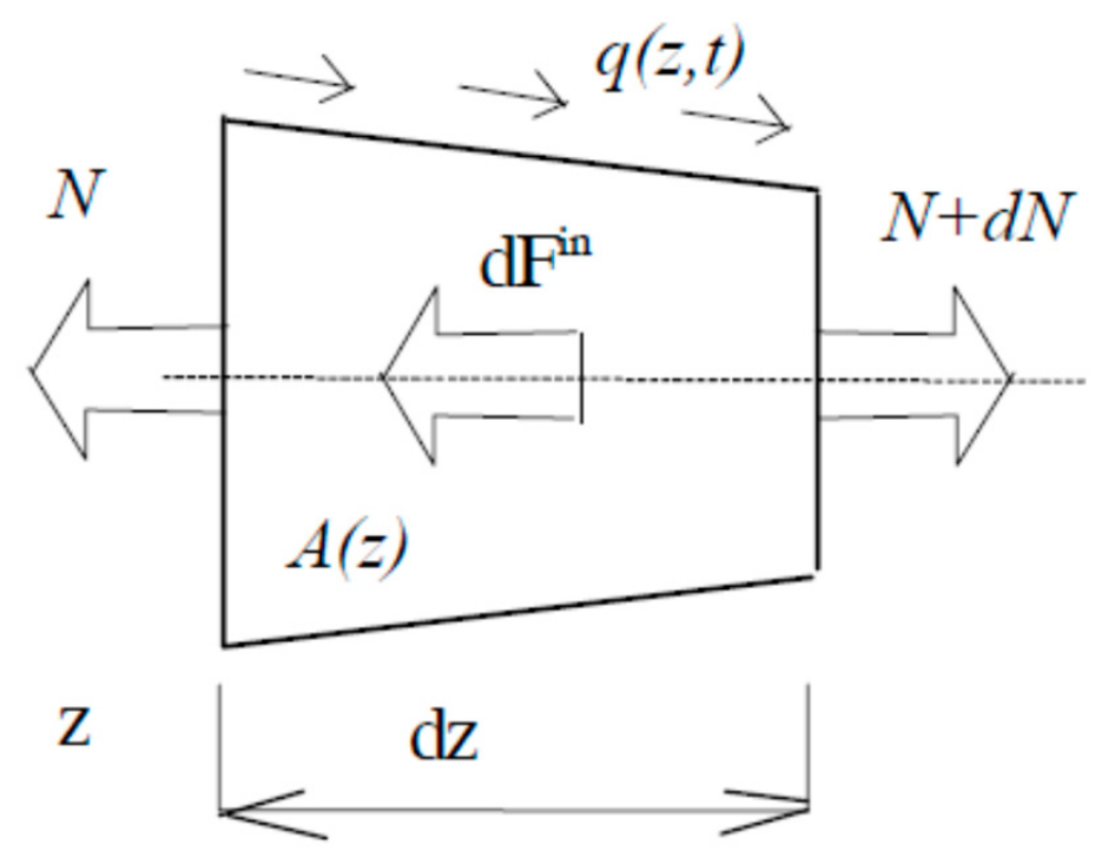
Normal force to the cross-section of the rheological Maxwell model of material, fractional type, with variable cross-section at coordinate $z\in \left(0.\mathcal{l}\right)$ is $N\left(z,t\right)=A\left(z\right)\sigma \left(z,t\right)$, while its value in cross-section on coordinate $z+dz\in \left(0.\mathcal{l}\right)$ is (see Figure 2): Normal force to the cross-section $A\left(z\right)$ of the rheological Maxwell model of material, fractional type, with variable cross-section $A\left(z\right)$ at coordinate $z\in \left(0.\mathcal{l}\right)$ is $N\left(z,t\right)=A\left(z\right)\sigma \left(z,t\right)$, while its value in cross-section on coordinate $z+dz\in \left(0.\mathcal{l}\right)$ is as follows (see Figure 2):

$$N\left(z+dz,t\right)=A\left(z\right)\sigma \left(z,t\right)+{\displaystyle \frac{\partial }{\partial z}}\left[A\left(z\right)\sigma \left(z,t\right)\right]dz$$

(12)

Let $w\left(z,t\right)$ denotes the longitudinal displacement of cross-section $A\left(z\right)$ of the rheologic Maxwell material–fractional type at longitudinal coordinate $z\in \left(0.\mathcal{l}\right)$. According to D’Alambert’s Principles of dynamical equilibrium of all acting forces on the system, the following differential equation could be written for dynamical equilibrium of the forces of one elementary part of rheologic Maxwell fractional-type material (for details see Reference [8]):

$$\rho A\left(z\right)dz{\displaystyle \frac{{\partial }^{2}w\left(z,t\right)}{\partial t^2}}=-N\left(z,t\right)+N\left(z+dz,t\right)+q\left(z,t\right)A\left(z\right)dz={\displaystyle \frac{\partial N\left(z,t\right)}{\partial z}}dz+q\left(z,t\right)A\left(z\right)dz$$

(13)

where $\rho$ is the viscoelastic rheological Maxwell model fractional-type material’s density, $A\left(z\right)$ is the area of cross-section of material flow, and $q\left(z,t\right)$ is the distributed volume force. Substituting Equation (12) into Equation (13) leads to the following:

$${\displaystyle \frac{{\partial }^{2}w\left(z,t\right)}{\partial t^2}}-{\displaystyle \frac{1}{\rho A\left(z\right)}}{\displaystyle \frac{\partial }{\partial z}}\left[A\left(z\right)\sigma \left(z,t\right)\right]={\displaystyle \frac{1}{\rho }}q\left(z,t\right)$$

(14)

We can now write two basic relations that describe the dynamics flow (creeping) of the rheological Maxwell model of a fractional-type material flowing (creeping) in a pipe of constant or variable cross-section: the first is the constitutive differential relation of the fractional order, and the second is the dynamic equilibrium equation of an element of the Maxwell model of a fractional-type material (14):

$${\displaystyle \frac{1}{E}}{\mathrm{D}}_t^{\alpha }\left[{\sigma }_z\left(z,t\right)\right]+{\displaystyle \frac{{\sigma }_z\left(z,t\right)}{E_{\alpha }}}=\left\{{\mathrm{D}}_t^{\alpha }\left[{\displaystyle \frac{\partial w\left(z,t\right)}{\partial z}}\right]\right\}\ne const, {\epsilon }_z\left(z,t\right)={\displaystyle \frac{\partial w\left(z,t\right)}{\partial t}}, 0<\alpha \le 1$$

(15)

$${\displaystyle \frac{{\partial }^{2}w\left(z,t\right)}{\partial t^2}}-{\displaystyle \frac{1}{\rho A\left(z\right)}}{\displaystyle \frac{\partial }{\partial z}}\left[A\left(z\right)\sigma \left(z,t\right)\right]={\displaystyle \frac{1}{\rho }}q\left(z,t\right)$$

(16)

From these Equations (15) and (16), we eliminate the longitudinal displacement $w\left(z,t\right)$, to obtain a partial differential equation of fractional order in terms of the nodal stress of rheological flow (creeping) of dynamics flow of the rheological Maxwell model of material, fractional type.

We differentiate the first fractional-order differential Equation (15) twice with respect to time. We then differentiate the second partial differential Equation (16) with respect to fractional-order time and with respect to the coordinate $z\in \left(0.\mathcal{l}\right)$ to obtain the following:

$${\displaystyle \frac{1}{E}}{\mathrm{D}}_t^{\alpha }\left[{\displaystyle \frac{{\partial }^2{\sigma }_z\left(z,t\right)}{\partial t^2}}\right]+{\displaystyle \frac{\frac{{\partial }^2{\sigma }_z\left(z,t\right)}{\partial t^2}}{E_{\alpha }}}=\left\{{\mathrm{D}}_t^{\alpha }\left[{\displaystyle \frac{{\partial }^{3}w\left(z,t\right)}{\partial z\partial t^2}}\right]\right\}\ne const, 0<\alpha \le 1$$

(17)

$${\mathrm{D}}_t^{\alpha }\left[{\displaystyle \frac{{\partial }^{3}w\left(z,t\right)}{\partial z\partial t^2}}\right]-{\displaystyle \frac{\partial }{\partial z}}〈{\displaystyle \frac{1}{\rho A\left(z\right)}}{\mathrm{D}}_t^{\alpha }\left[{\displaystyle \frac{\partial }{\partial z}}\left[A\left(z\right)\sigma \left(z,t\right)\right]\right]〉={\displaystyle \frac{1}{\rho }}{\displaystyle \frac{\partial }{\partial z}}〈{\mathrm{D}}_t^{\alpha }\left[q\left(z,t\right)\right]〉$$

(18)

Then, we substitute the first obtained Equation (17) into the second (18), and we obtain a partial differential equation of fractional order in terms of the normal stress $\sigma \left(z,t\right)$ in the following form:

$${\displaystyle \frac{1}{E}}{\mathrm{D}}_t^{\alpha }\left[{\displaystyle \frac{{\partial }^2{\sigma }_z\left(z,t\right)}{\partial t^2}}\right]+{\displaystyle \frac{\frac{{\partial }^2{\sigma }_z\left(z,t\right)}{\partial t^2}}{E_{\alpha }}}-{\displaystyle \frac{\partial }{\partial z}}〈{\displaystyle \frac{1}{\rho A\left(z\right)}}{\mathrm{D}}_t^{\alpha }\left[{\displaystyle \frac{\partial }{\partial z}}\left[A\left(z\right)\sigma \left(z,t\right)\right]\right]〉={\displaystyle \frac{1}{\rho }}{\displaystyle \frac{\partial }{\partial z}}〈{\mathrm{D}}_t^{\alpha }\left[q\left(z,t\right)\right]〉$$

(19)

This fractional-order partial differential Equation (19) in terms of normal stress describes the longitudinal dynamics flow (creeping) of the rheological Maxwell model of a fractional-type material in a pipe of constant or variable cross-section as a function of the longitudinal coordinate.

4. Decomposition of the Partial Differential Equation of Longitudinal Flow Dynamics of the Maxwell Model of a Material

Let us assume the solution of the partial differential Equation (19) of fractional order of the longitudinal dynamics-flow of the rheological Maxwell model of the fractional-type material in a pipe of variable cross-section under normal stress in the form of the product of two functions, one $T\left(t\right)$ that depends on time $t$, and the other $Z\left(z\right)$ that depends on the longitudinal coordinate $z\in \left(0.\mathcal{l}\right)$ in the following form:

$${\sigma }_z\left(z,t\right)=Z\left(z\right)T\left(t\right)$$

(20)

Assume that the load is in the form $q\left(z,t\right)=Z\left(z\right)Q\left(t\right)$, the resulting equation is in the following form:

$${\displaystyle \frac{Z\left(z\right)}{E}}{\mathrm{D}}_t^{\alpha }\left[{\displaystyle \frac{{\partial }^2\left(T\left(t\right)\right)}{\partial t^2}}\right]+Z\left(z\right){\displaystyle \frac{\frac{{\partial }^2\left(T\left(t\right)\right)}{\partial t^2}}{E_{\alpha }}}-{\displaystyle \frac{\partial }{\partial z}}〈{\displaystyle \frac{1}{\rho A\left(z\right)}}{\displaystyle \frac{\partial }{\partial z}}\left[A\left(z\right)\left(Z\left(z\right)\right)\right]{\mathrm{D}}_t^{\alpha }\left[T\left(t\right)\right]〉={\displaystyle \frac{1}{\rho }}{\displaystyle \frac{\partial Z\left(z\right)}{\partial z}}〈{\mathrm{D}}_t^{\alpha }\left[Q\left(t\right)\right]〉$$

(21)

Then, we separate the resulting Equation (21) into two separate ordinary differential equations, one in terms of a function in terms $Z\left(z\right)$ of coordinates $z\in \left(0.\mathcal{l}\right)$, and the other of fractional order in terms of a function in terms $z\in \left(0.\mathcal{l}\right)$ of time $t$. For that reason, we divide the differential Equation (21) by $Z\left(z\right)$ and separate the left and right sides into terms $T\left(t\right)$ that depend only on time, i.e., only on the coordinate $Z\left(z\right)$:

$${\mathrm{D}}_t^{\alpha }\left[{\displaystyle \frac{{\partial }^2\left(T\left(t\right)\right)}{\partial t^2}}\right]+{\displaystyle \frac{E}{E_{\alpha }}}{\displaystyle \frac{{\partial }^2\left(T\left(t\right)\right)}{\partial t^2}}\mp k^{2}E{\mathrm{D}}_t^{\alpha }\left[T\left(t\right)\right]={\displaystyle \frac{E}{\rho }}{\displaystyle \frac{1}{Z\left(z\right)}}{\displaystyle \frac{\partial Z\left(z\right)}{\partial z}}〈{\mathrm{D}}_t^{\alpha }\left[Q\left(t\right)\right]〉$$

(22)

$$-{\displaystyle \frac{\partial }{Z\left(z\right)\partial z}}〈{\displaystyle \frac{1}{\rho A\left(z\right)}}{\displaystyle \frac{\partial }{\partial z}}\left[A\left(z\right)\left(Z\left(z\right)\right)\right]〉==\pm k^2$$

(23)

We have separated the partial differential Equation (21) of fractional order, in the form of two separate ones, (22) in (23), one ordinary differential equation in terms of the function in terms $Z\left(z\right)$ of the coordinate $z\in \left(0.\mathcal{l}\right)$, and the other of fractional order in terms of the function $T\left(t\right)$ in terms of time $t$, where we have introduced one unknown constant $+k^2$, which we determine from the condition that the function $Z\left(z\right)$ in terms of the coordinate $z\in \left(0.\mathcal{l}\right)$ as well as the solution for the flows normal stress $\sigma \left(z,t\right)$ of floe (creeping) of rheological Maxwell’s material satisfy the boundary conditions. Now we can write the previous system of Equations (22) and (23) in the following convenient form:

$$T^{″}\left(t\right)+{\displaystyle \frac{E_{\alpha }}{E}}{\mathrm{D}}_t^{\alpha }\left[T^{″}\left(t\right)\right]\mp k^2{E}_{\alpha }{\mathrm{D}}_t^{\alpha }\left[T\left(t\right)\right]={\displaystyle \frac{E_{\alpha }}{\rho }}{\displaystyle \frac{Z^{\prime }\left(z\right)}{Z\left(z\right)}}〈{\mathrm{D}}_t^{\alpha }\left[Q\left(t\right)\right]〉$$

(24)

$$-{\displaystyle \frac{\partial }{Z\left(z\right)\partial z}}〈{\displaystyle \frac{1}{\rho A\left(z\right)}}{\displaystyle \frac{\partial }{\partial z}}\left[A\left(z\right)\left(Z\left(z\right)\right)\right]〉==\pm k^2$$

(25)

In the previous system of ordinary differential Equations (24) and (25), the first of which is of fractional order, we have introduced the eigen-characteristic number $+k^2$, which we determine from the boundary conditions, which will be explained in the following sections of the article.

The previous first ordinary differential Equation (24) in terms of the eigen-time function is an ordinary differential equation of fractional order, and from it we determine the eigen-time functions $T\left(t\right)$. The second Equation (25) is an ordinary differential equation in terms of functions $T\left(t\right)$ that depend on the longitudinal coordinate $Z\left(z\right)$ and from it we determine the eigen-amplitude functions, which must satisfy the boundary conditions. The sign in front of the constant is determined from the condition that the solution for the eigen-amplitude function that depends on the longitudinal coordinate в $z\in \left(0.\mathcal{l}\right)$, satisfies the conditions of physical reality of the task of mathematical solution of the ordinary differential Equation (25).

In the paper, we assumed that it is possible to differentiate over whole derivatives and derivatives of fractional order by changing the order of differentiation.

5. Eigen-Amplitude Functions for the Realization of Flow Dynamics

It is necessary to solve the ordinary differential Equation (25) by its own amplitude function $Z\left(z\right)$ for each selected cross-sectional shape $A\left(z\right)$, which we express in function of the longitudinal coordinate $z$, as well as for the corresponding boundary conditions by normal stress ${\sigma }_z\left(z,t\right)=Z\left(z\right)T\left(t\right)$, for flows of the rheological Maxwell model of fractional-type material in a pipe of variable cross-section $A\left(z\right)$:

$$Z^{″}\left(z\right)+{\displaystyle \frac{\partial }{\partial z}}〈{\displaystyle \frac{A^{\prime }\left(z\right)}{A\left(z\right)}}Z\left(z\right)〉\pm \rho k^{2}Z\left(z\right)=0$$

(26)

In this section, we will analyze the solutions to the differential Equation (26) for selected cross-sections $A\left(z\right)$ and some of the boundary conditions for the normal stresses ${\sigma }_z\left(z,t\right)=Z\left(z\right)T\left(t\right)$ for the flow of the rheological Maxwell material model of fractional type.

5.1* As the simplest case of flow of the rheological Maxwell model of the fractional-type material, we choose a constant cross-section $A\left(z\right)=A_0=vpnst$, along the longitudinal coordinate. Then this differential Equation (26) in terms of its own amplitude function becomes the following:

$$Z^{″}\left(z\right)\pm \rho k^{2}Z\left(z\right)=0$$

(27)

The mathematical solutions of the previous ordinary differential Equation (27) in terms of its own amplitude function $Z\left(z\right)$ are as follows:

$$Z\left(z\right)=C_1\mathit{cos}k\sqrt{\rho }z+C_2\mathit{sin}k\sqrt{\rho }z$$

(28)

and

$$Z\left(z\right)=C_{1}chk\sqrt{\rho }z+C_{2}shk\sqrt{\rho }z$$

(29)

The first mathematical solution (28) corresponds to the physical properties of the problem of the flow of the rheological Maxwell model of material, fractional type in a pipe, so we write the eigen-characteristic constant $+k^2$ with a plus sign.

* If the pipe is free at both ends and means that the normal stresses ${\sigma }_z\left(z,t\right)=Z\left(z\right)T\left(t\right)$ in the cross-sections $A\left(z\right)=A_0=vpnst$ at both ends, in the corresponding cross-sections $A\left(z\right)$ for $z_0=0$ and for $z_k=\mathcal{l}$, are zero, for the flow of the rheological Maxwell model of material, fractional type, so the amplitude functions of the eigenvalues at the ends of the pipe are equal to zero: $Z\left(0\right)=0$ and $Z\left(\mathcal{l}\right)=0$. From these conditions, the following applies:

$$\begin{array}{cc}Z\left(0\right)=C_1=0, Z\left(\mathcal{l}\right)& =C_2\mathit{sin}k\sqrt{\rho }\mathcal{l}=0\Rightarrow k\sqrt{\rho }\mathcal{l}=n\pi ,\hspace{1em}n=0,1,2,4,\dots ,\propto \hfill \\ & \Rightarrow n=0,1,2,4,\dots ,\propto k_n\sqrt{\rho }=\hspace{0.17em}{\displaystyle \frac{n\pi }{\mathcal{l}}}\hfill \end{array}$$

(30)

Thus, we have determined the eigen-characteristic numbers, $k_n\sqrt{\rho }=\hspace{0.17em}{\displaystyle \frac{n\pi }{\mathcal{l}}}$, $n=0,1,2,4,\dots ,\propto$, of which there are infinitely many, for the observed flow (creeping) of the rheological Maxwell model of a fractional-type material in a pipe of constant cross-section. For each characteristic number, the eigen-amplitude function $Z\left(z\right)$ for the flow of the rheological Maxwell model of a fractional-type material is of the following form:

$$Z{}_s\left(z\right)=C_{2,s}\mathit{sin}{k}_s\sqrt{\rho }z=C_{2,s}\mathit{sin}{\displaystyle \frac{s\pi }{\mathcal{l}}}z, s=0,1,2,4,\dots ,\propto$$

(31)

This means that there are infinitely many proper amplitude forms $Z\left(z\right)$ and that they are of the form (31), $Z{}_s\left(z\right)=C_{2,s}\mathit{sin}{k}_{s}z=C_{2,s}\mathit{sin}{\displaystyle \frac{s\pi }{\mathcal{l}}}z$, $s=0,1,2,4,\dots ,\propto$. They also correspond to each proper characteristic number from the set $k_n=\hspace{0.17em}{\displaystyle \frac{n\pi }{\mathcal{l}\sqrt{\rho }}}$, $n=0,1,2,4,\dots ,\propto$.

The sets of eigenvalue functions (31), $Z{}_s\left(z\right)=C_{2,s}\mathit{sin}{k}_s\sqrt{\rho }z=C_{2,s}\mathit{sin}{\displaystyle \frac{s\pi }{\mathcal{l}}}z$, $s=0,1,2,4,\dots ,\propto$ and $Z{}_n\left(z\right)=C_{2,n}\mathit{sin}{k}_n\sqrt{\rho }z=C_{2,s}\mathit{sin}{\displaystyle \frac{n\pi }{\mathcal{l}}}z$, $n=0,1,2,4,\dots ,\propto$, for the flow (creeping) of the rheological Maxwell model of a fractional-type material in a pipe of constant cross-section, satisfy the orthogonality conditions:

$${\displaystyle {\displaystyle \underset{0}{\overset{\mathcal{l}}{\int }}}Z{}_n\left(z\right)Z{}_s\left(z\right)dz=\left\{\begin{array}{c}0\hspace{1em}n\ne s\\ m_{n⋮}\hspace{1em}s=n\end{array}\right.}$$

(32)

These orthogonality conditions (32), in the general case for the flow of the rheological Maxwell model of a fractional-type material in a pipe of variable cross-section, can be obtained from the differential Equation (27) itself by the eigen-amplitude functions $Z_s\left(z\right)$, $s=1,2,3,\dots ,\infty$. It is sufficient to multiply the differential Equation (27) twice by two different indices, $s=1,2,3,\dots ,\infty$ and $n=0,1,2,4,\dots ,\propto$. Then, multiply the first by, and the second by $Z_s\left(z\right)$, $s=1,2,3,\dots ,\infty$, subtract them—i.e., the first from the second—and then integrate them along the longitudinal coordinate from zero to the next end of the pipe, from $z_0=0$ to $z_k=\mathcal{l}$. In the obtained result, through multiple repeated partial integrations and entering different values of the eigen-amplitude functions—$Z_n\left(z\right)$, $n=0,1,2,4,\dots ,\propto$, and $Z_s\left(z\right)$, $s=1,2,3,\dots ,\infty$—at the boundaries of the intervals, for $z_0=0$ and for $z_k=\mathcal{l}$, we obtain the conditions of orthogonality of the eigen-amplitude functions:

$$Z_s^{″}\left(z\right)+{\displaystyle \frac{A^{\prime }\left(z\right)}{A\left(z\right)}}{Z}_s^{\prime }\left(z\right)+〈{\displaystyle \frac{\partial }{\partial z}}\left[{\displaystyle \frac{A^{\prime }\left(z\right)}{A\left(z\right)}}\right]\pm \rho k^2〉Z_s\left(z\right)=0, s=1,2,3,\dots ,\infty$$

(33)

$$Z_n^{″}\left(z\right)+{\displaystyle \frac{A^{\prime }\left(z\right)}{A\left(z\right)}}{Z}_n^{\prime }\left(z\right)+〈{\displaystyle \frac{\partial }{\partial z}}\left[{\displaystyle \frac{A^{\prime }\left(z\right)}{A\left(z\right)}}\right]\pm \rho k^2〉Z_n\left(z\right)=0, n=0,1,2,4,\dots ,\propto$$

(34)

The result of the subtraction is as follows:

$$〈Z_s^{″}\left(z\right)Z_n\left(z\right)-Z_n^{″}\left(z\right)Z_s\left(z\right)〉+{\displaystyle \frac{A^{\prime }\left(z\right)}{A\left(z\right)}}\left[Z_s^{\prime }\left(z\right)Z_n\left(z\right)-Z_n^{\prime }\left(z\right)Z_s\left(z\right)\right]=0$$

(35)

Then, following the partial integration in several stages, with the introduction of the general possible boundary conditions of the considered problem, we obtain the following:

$$\begin{array}{l}{\displaystyle {\int }_0^{\mathcal{l}}〈Z_s^{″}\left(z\right)Z_n\left(z\right)-Z_n^{″}\left(z\right)Z_s\left(z\right)〉dz}+\\ \hspace{1em}+{\displaystyle {\int }_0^{\mathcal{l}}〈\frac{A^{\prime }\left(z\right)}{A\left(z\right)}\left[Z_s^{\prime }\left(z\right)Z_n\left(z\right)-Z_n^{\prime }\left(z\right)Z_s\left(z\right)\right]〉dz}=0=0\end{array}$$

(36)

These, as a final result, follow the orthogonality conditions of the eigen-amplitude functions in the general form (32).

For this case, for the flow (creeping) of the rheological Maxwell model of a fractional-type material in a pipe of constant cross-section, when we have determined the eigen-amplitude functions $Z{}_n\left(z\right)=C_{2,n}\mathit{sin}{k}_n\sqrt{\rho }z=C_{2,s}\mathit{sin}{\displaystyle \frac{n\pi }{\mathcal{l}}}z$, $n=0,1,2,4,\dots ,\propto$ in the form (31), we can check the orthogonality conditions by direct calculation and obtain the following:

$${\displaystyle {\displaystyle \underset{0}{\overset{\mathcal{l}}{\int }}}Z{}_n\left(z\right)Z{}_s\left(z\right)dz={\displaystyle {\displaystyle \underset{0}{\overset{\mathcal{l}}{\int }}}{C}_{2,s}\mathit{sin}\frac{n\pi }{\mathcal{l}}z{C}_{2,s}\mathit{sin}\frac{s\pi }{\mathcal{l}}zdz}=\left\{\begin{array}{c}0\hspace{1em}n\ne s\\ m_{n⋮}=\frac{1}{2}{C}_{2,n}^2\hspace{1em}s=n\end{array}\right.}$$

(37)

5.2* If for a variable cross-section of a pipe for the flow of a rheological Maxwell’s fractional-type material model in a pipe of variable cross-section we adopt a circular cross-section $A\left(z\right)$ with a diameter, which changes along the longitudinal coordinate $z$ as follows:

$$d\left(z\right)=D_1\left(1-\beta z\right)$$

(38)

Hence, the cross-sectional area $A\left(z\right)$ is $A\left(z\right)={\displaystyle \frac{d^2\left(z\right)\pi }{4}}={\displaystyle \frac{1}{4}}{D}_1^2{\left(1-\beta z\right)}^2$. The following applies:

$${\displaystyle \frac{A^{\prime }\left(z\right)}{A\left(z\right)}}=-{\displaystyle \frac{\frac{1}{4}{D}_1^{2}2\left(1-\beta z\right)\alpha z}{\frac{1}{4}{D}_1^2{\left(1-\beta z\right)}^2}}=-{\displaystyle \frac{2\beta }{\left(1-\beta z\right)}}$$

(39)

The differential Equation (26) in terms of the eigen-amplitude functions $Z\left(z\right)$ for the flow of the rheological Maxwell model of the material, fractional type, for this case of changing the circular cross-section (38) of the pipe is as follows:

$$Z^{″}\left(z\right)-{\displaystyle \frac{2\beta }{\left(1-\beta z\right)}}{Z}^{\prime }\left(z\right)+\left({\displaystyle \frac{2{\beta }^2}{{\left(1-\beta z\right)}^2}}\pm \rho k^2\right)Z\left(z\right)=0$$

(40)

5.3* If for the variable cross-section $A\left(z\right)$ of a pipe for the flow of a rheological Maxwell fractional-type material model in a pipe of variable cross-section $A\left(z\right)$ we adopt a circular cross-section with a diameter that varies along the longitudinal coordinate $z$ as follows:

$$d\left(z\right)=D_1{e}^{-\delta z}$$

(41)

So, the cross-sectional area is $A\left(z\right)={\displaystyle \frac{d^2\left(z\right)\pi }{4}}={\displaystyle \frac{1}{4}}{D}_1^2{e}^{{-2\delta z}^2}$, which relates to the following:

$${\displaystyle \frac{A^{\prime }\left(z\right)}{A\left(z\right)}}=-{\displaystyle \frac{\frac{1}{4}{D}_1^{2}2\delta e^{-2\delta z}}{\frac{1}{4}{D}_1^2{e}^{-2\delta z}}}={\displaystyle \frac{2\delta e^{-2\delta z}}{e^{-2\delta z}}}=-2\delta , {\displaystyle \frac{\partial }{\partial z}}〈{\displaystyle \frac{A^{\prime }\left(z\right)}{A\left(z\right)}}Z\left(z\right)〉=-2\delta Z^{\prime }\left(z\right)$$

(42)

The differential Equation (26) in terms of the eigen-amplitude functions $Z\left(z\right)$ for the flow of the rheological Maxwell model of the material, fractional type, for this case of changing the circular cross-section (41) of the pipe is as follows:

$$Z^{″}\left(z\right)-2\delta Z^{\prime }\left(z\right)\pm \rho k^{2}Z\left(z\right)=0$$

(43)

To solve the previous differential Equation (43), we introduce a shift in the following form:

$$Z\left(z\right)=Z{}_a\left(z\right)e^{\delta z}$$

(44)

Then, we differentiate the previously introduced solution with respect to the longitudinal coordinate to obtain the following:

$$Z^{\prime }\left(z\right)=Z^{\prime }{}_a\left(z\right)e^{\delta z}+\delta Z{}_a\left(z\right)e^{\delta z}$$

(45)

$$Z^{″}\left(z\right)=Z^{″}{}_a\left(z\right)e^{\delta z}+\delta Z^{\prime }{}_a\left(z\right)e^{\delta z}+\delta Z^{\prime }{}_a\left(z\right)e^{\delta z}+{\delta }^{2}Z{}_a\left(z\right)e^{\delta z}$$

(46)

We multiply the assumed solution (44) by $\left(\pm \rho k^2\right)$ and the first derivative (45) by $\left(-2\delta \right)$ and then add them to the second derivative (46) to obtain the following classical differential equation with constant coefficients:

$$Z^{″}{}_a\left(z\right)e^{\delta z}+Z{}_a\left(z\right)e^{\delta z}\left(\pm \rho k^2+2{\delta }^2\right)=0$$

(47)

When we divide by $e^{\delta z}$, we obtain an unknown differential equation in the following form:

$$Z^{″}{}_a\left(z\right)+Z{}_a\left(z\right)\left(\pm \rho k^2+2\delta \right)=0$$

(48)

The mathematical solutions of the previous differential Equation (48) are in the following forms:

$$Z{}_a\left(z\right)=Z\left(z\right)e^{-\delta z}=C_1\mathit{cos}z\sqrt{\left(2\delta \pm \rho k^2\right)}+C_{2}sunz\sqrt{\left(2\delta \pm \rho k^2\right)}$$

(49)

and

$$Z_a=Z\left(z\right)e^{-\delta z}=C_{1}chz\sqrt{\left(2\delta \pm \rho k^2\right)}+C_{2}shz\sqrt{\left(2\delta \pm \rho k^2\right)}$$

(50)

For the eigen-amplitude functions $Z\left(z\right)$, for the flow (creeping) of the rheological Maxwell model of fractional-type material, and for this case of changing the circular cross-section of a pipe of diameter (41), the corresponding solution is as follows:

$$Z\left(z\right)=Z{}_a\left(z\right)e^{\delta z}=\left[C_1\mathit{cos}z\sqrt{\left(2\delta \pm \rho k^2\right)}+C_{2}sunz\sqrt{\left(2\delta \pm \rho k^2\right)}\right]e^{\delta z}$$

(51)

These are the solutions of the differential Equation (45).

The eigen-characteristic number $p^2$, that is $p^2$, is in the following form:

$$p^2=\left(\pm \rho k^2+2\delta \right)\mathrm{that} \mathrm{is}, p=\sqrt{\left(2\delta \pm \rho k^2\right)}$$

(52)

We consider the boundary conditions where both ends of the tube are free. Then, the normal stresses, ${\sigma }_z\left(z,t\right)=Z\left(z\right)T\left(t\right)$, in the sections at both ends ($z_0=0$ and $z_k=\mathcal{l}$), in the corresponding cross-sections, are simply zero, and it follows that the eigenvalue functions, $Z\left(0\right)=0$ and $Z\left(\mathcal{l}\right)=0$, are equal to zero:

$$Z\left(0\right)=0\mathrm{and} Z\left(\mathcal{l}\right)=0$$

(53)

These conditions (53) are the boundary conditions, which follow from the conditions for normal stresses ${\sigma }_z\left(z,t\right)=Z\left(z\right)T\left(t\right)$ at the ends of the pipe for the flow (creeping) of the rheological Maxwell model of a fractional-type material, and are equal to zero.

Since the eigen-amplitude functions of the form (51) are $Z\left(z\right)$, by applying the boundary conditions (53), we write the following:

$$\begin{array}{c}Z\left(0\right)=C_1=0, Z\left(\mathcal{l}\right)=C_{2}sun\mathcal{l}\sqrt{\left(2\delta \pm \rho k_n^2\right)}\mathcal{l}{e}^{\delta }=0\hfill \\ \Rightarrow \mathcal{l}\sqrt{\left(2\delta \pm \rho k^2\right)}=n\pi ,\hspace{1em}n=0,1,2,4,\dots ,\propto \hfill \\ \Rightarrow n=0,1,2,4,\dots ,\propto , \sqrt{\left(2\delta \pm \rho k_n^2\right)}=\hspace{0.17em}{\displaystyle \frac{n\pi }{\mathcal{l}}}\hfill \end{array}$$

(54)

In other words, the following applies:

$$k_n\sqrt{\rho }=\sqrt{p_n^2-2\delta }=\sqrt{{\left({\displaystyle \frac{n\pi }{\mathcal{l}}}\right)}^2-2\delta }, n=0,1,2,4,\dots ,\propto$$

(55)

The eigen-characteristic flow numbers of the rheological Maxwell model of fractional-type material through a pipe of variable circular cross-section of diameter (41) are as follows:

$$k_n=\sqrt{{\displaystyle \frac{\left(p_n^2-2\delta \right)}{\rho }}}=\sqrt{{\displaystyle \frac{{\left(\frac{n\pi }{\mathcal{l}}\right)}^2-2\delta }{\rho }}}. n=0,1,2,4,\dots ,\propto$$

(56)

The eigen-amplitude functions are of the following form:

$$Z{}_s\left(z\right)=C_{2,s}{e}^{\delta \mathcal{l}}\mathit{sin}z\sqrt{\left(2\delta \pm \rho k_s^2\right)}=C_{2,s}{e}^{\delta \mathcal{l}}\mathit{sin}{\displaystyle \frac{s\pi }{\mathcal{l}}}z, s=0,1,2,4,\dots ,\propto$$

(57)

Notably, their amounts are infinite.

From the form (57) of the eigen-amplitude forms, $Z{}_n\left(z\right)=C_{2,n}{e}^{\delta \mathcal{l}}\mathit{sin}z\sqrt{\left(2\delta \pm \rho k_n^2\right)}=C_{2,n}{e}^{\delta \mathcal{l}}\mathit{sin}{\displaystyle \frac{n\pi }{\mathcal{l}}}z$, $s=0,1,2,4,\dots ,\propto$, and that each corresponds to one of the set of many eigen-characteristic numbers, $p_n=\sqrt{\left(2\delta +\rho k_n^2\right)}$, $n=0,1,2,4,\dots ,\propto$, or $k_n^2={\displaystyle \frac{1}{\rho }}\left(p_n^2-2\delta \right)$, or $k_n={\displaystyle \frac{1}{\sqrt{\rho }}}\sqrt{p_n^2-2\delta }={\displaystyle \frac{1}{\sqrt{\rho }}}\sqrt{{\left({\displaystyle \frac{n\pi }{\mathcal{l}}}\right)}^2-2\delta }$, for the flow (creeping) of the rheological Maxwell model of fractional-type material through a pipe of variable cross-section diameter (41) and that they grow exponentially with the longitudinal coordinate.

The eigen-amplitude functions, $Z{}_n\left(z\right)=C_{2,n}{e}^{\delta \mathcal{l}}\mathit{sin}z\sqrt{\left(2\delta \pm \rho k_n^2\right)}=C_{2,s}{e}^{\delta \mathcal{l}}\mathit{sin}{\displaystyle \frac{n\pi }{\mathcal{l}}}z$, $s=0,1,2,4,\dots ,\propto$ and $Z{}_n\left(z\right)=C_{2,n}{e}^{\delta \mathcal{l}}\mathit{sin}z\sqrt{\left(2\delta \pm \rho k_n^2\right)}=C_{2,n}{e}^{\delta \mathcal{l}}\mathit{sin}{\displaystyle \frac{n\pi }{\mathcal{l}}}z$, $n=0,1,2,4,\dots ,\propto$, of the flow (creeping) of the rheological Maxwell model of a fraction-type material through a pipe of variable cross-section of diameter (41) satisfy the orthogonality conditions (32), which in this case can also be proved from the differential equation of the eigen-amplitude functions $Z{}_n\left(z\right)=C_{2,n}{e}^{\delta \mathcal{l}}\mathit{sin}z\sqrt{\left(2\delta \pm \rho k_n^2\right)}=C_{2,s}{e}^{\delta \mathcal{l}}\mathit{sin}{\displaystyle \frac{n\pi }{\mathcal{l}}}z$, $n=0,1,2,4,\dots ,\propto$, or by direct integration. For this case, we obtain the following:

$${\displaystyle {\displaystyle \underset{0}{\overset{\mathcal{l}}{\int }}}Z{}_n\left(z\right)Z{}_s\left(z\right)dz={\displaystyle {\displaystyle \underset{0}{\overset{\mathcal{l}}{\int }}}{C}_{2,s}{e}^{\delta \mathcal{l}}\mathit{sin}\frac{n\pi }{\mathcal{l}}z{C}_{2,s}\mathit{sin}\frac{s\pi }{\mathcal{l}}zdz}=\left\{\begin{array}{c}0\hspace{1em}n\ne s\\ m_{n⋮2,n}^2\hspace{1em}s=n\end{array}\right.}$$

(58)

We have shown in several examples that both the differential equation in terms of its own amplitude function $Z\left(z\right)$ and in terms of the longitudinal coordinate $z$ can be separated and can be immediately solved independently of the ordinary differential equation of fractional order in terms of $T\left(t\right)$ its own time function $T\left(t\right)$ that depends on time $t$. We have previously shown the solution of the second ordinary differential Equation (25) or (26) in examples, taking into account that the solution is performed for each case of a change in the cross-section of the pipe individually and for each case individually selected boundary conditions according to the normal flow stresses of the rheological Maxwell model of the material, fractional type.

5.4* Overview of possible boundary conditions for the longitudinal flow dynamics of a rheological Maxwell material model, fractional type, in a pipe of variable cross-section.

In this section, we will list some more possible boundary conditions for the longitudinal flow dynamics of a rheological Maxwell model of a fraction-type material in a pipe of constant or variable cross-section.

The solutions for the eigen-amplitude functions $Z\left(z\right)$, which we have shown in the previous three examples, for selected pipe cross-sections, must satisfy the boundary conditions.

We determine the boundary conditions for each specific case of the choice of changes in pipe cross-sections along the longitudinal coordinate $z$, as well as at each end of the pipe for $z_0=0$ and $z_k=\mathcal{l}$.

* For a tube fixed at the left end ($z_0=0$) and free at the right end ($z_k=\mathcal{l}$), the normal stress ${\sigma }_z\left(z,t\right)=Z\left(z\right)T\left(t\right)$ at the free end ($z_0=0$) is equal to the axial force divided by the cross-sectional area: ${\sigma }_z\left(z_0,t\right)=Z\left(z_0\right)T\left(t\right)={\displaystyle \frac{F{}_{a,0}T\left(t\right)}{A\left(z_0\right)}}$.

The normal stress ${\sigma }_z\left(z,t\right)=Z\left(z\right)T\left(t\right)$ at the free end ($z_k=\mathcal{l}$) is equal to zero (${\sigma }_z\left(\mathcal{l},t\right)=Z\left(\mathcal{l}\right)T\left(t\right)=0$), and it follows that the eigen-amplitude function $Z\left(z\right)$ at that end is equal to zero.

These boundary conditions are as follows:

$$Z\left(z_0\right)\backslash ={\displaystyle \frac{F_{a,0}}{A\left(z_0\right)}} \mathrm{and} Z\left(\mathcal{l}\right)=0$$

(59a)

* When the pipe is fixed at both ends, the normal stresses ${\sigma }_z\left(z,t\right)=Z\left(z\right)T\left(t\right)$ in the sections at both ends ($z_0=0$ and $z_k=\mathcal{l}$) are equal to the corresponding axial forces divided by the corresponding cross-sections area. The boundary conditions are of the following form:

$${\sigma }_z\left(z_0,t\right)=Z\left(z_0\right)T\left(t\right)={\displaystyle \frac{F{}_{a,0}T\left(t\right)}{A\left(z_0\right)}}\Rightarrow Z\left(z_0\right)\backslash ={\displaystyle \frac{F_{a,0}}{A\left(z_0\right)}}$$

(59b)

$${\sigma }_{\mathcal{l}}\left(z_{\mathcal{l}},t\right)=Z\left(z_{\mathcal{l}}\right)T\left(t\right)={\displaystyle \frac{F{}_{a,\mathcal{l}}T\left(t\right)}{A\left(z_{\mathcal{l}}\right)}}\Rightarrow Z\left(z_{\mathcal{l}}\right)={\displaystyle \frac{F{}_{a,\mathcal{l}}T\left(t\right)}{A\left(z_{\mathcal{l}}\right)}}$$

(60)

* When the pipe is free at both ends, the normal stresses ${\sigma }_z\left(z,t\right)=Z\left(z\right)T\left(t\right)$ in the corresponding cross-sections at both ends ($z_0=0$ and $z_k=\mathcal{l}$) are zero. It follows that the eigen-amplitude functions $Z\left(z\right)$ in the cross-sections at the ends of the pipe are equal to zero, and the boundary conditions are in the following form:

$$Z\left(0\right)=0\mathrm{and} Z\left(\mathcal{l}\right)=0$$

(61)

* When a pipe is fixed at the left end ($z_0=0$) while carrying a material point at the right end ($z_k=\mathcal{l}$), the normal stress, ${\sigma }_z\left(z,t\right)=Z\left(z\right)T\left(t\right)$, of the left end is equal to the axial force divided by the cross-sectional area: ${\sigma }_z\left(z_0,t\right)=Z\left(z_0\right)T\left(t\right)={\displaystyle \frac{F{}_{a,0}T\left(t\right)}{A\left(z_0\right)}}$, $Z\left(z_0\right)\backslash ={\displaystyle \frac{F_{a,0}}{A\left(z_0\right)}}$. For the normal stress ${\sigma }_z\left(z,t\right)=Z\left(z\right)T\left(t\right)$ at the right end ($z_k=\mathcal{l}$), it is equal to the inertia force divided by the cross-sectional area: ${\sigma }_z\left(\mathcal{l},t\right)=Z\left(\mathcal{l}\right)T\left(t\right)=-〈-{\displaystyle \frac{m_{\mathcal{l}}}{A\left(\mathcal{l}\right)}}{\displaystyle \frac{{\partial }^{2}w\left(\mathcal{l},t\right)}{\partial t^2}}〉$. In this case, the boundary conditions are as follows:

$$Z\left(z_0\right)\backslash ={\displaystyle \frac{F_{a,0}}{A\left(z_0\right)}} \mathrm{and} {\sigma }_z\left(\mathcal{l},t\right)=Z\left(\mathcal{l}\right)T\left(t\right)=-〈-{\displaystyle \frac{m_{\mathcal{l}}}{A\left(\mathcal{l}\right)}}{\displaystyle \frac{{\partial }^{2}w\left(\mathcal{l},t\right)}{\partial t^2}}〉$$

(62)

* In a tube that carries one material point at both ends, the left ($z_0=0$) and right ($z_k=\mathcal{l}$) ends, with masses $m_0$ and $m_{\mathcal{l}}$, the normal stresses at the ends are equal to the corresponding inertia force divided by the corresponding cross-section, ${\displaystyle \frac{m_0}{A\left(0\right)}}{\displaystyle \frac{{\partial }^{2}w\left(0,t\right)}{\partial t^2}}$, i.e., the inertia force divided by the cross-section of the right end $〈{\displaystyle \frac{m_{\mathcal{l}}}{A\left(\mathcal{l}\right)}}{\displaystyle \frac{{\partial }^{2}w\left(\mathcal{l},t\right)}{\partial t^2}}〉$. The boundary conditions in this case are in the following form:

$${\sigma }_z\left(0,t\right)=Z\left(0\right)T\left(t\right)={\displaystyle \frac{m_0}{A\left(0\right)}}{\displaystyle \frac{{\partial }^{2}w\left(0,t\right)}{\partial t^2}} \mathrm{and} {\sigma }_z\left(\mathcal{l},t\right)=Z\left(\mathcal{l}\right)T\left(t\right)=--〈{\displaystyle \frac{m_{\mathcal{l}}}{A\left(\mathcal{l}\right)}}{\displaystyle \frac{{\partial }^{2}w\left(\mathcal{l},t\right)}{\partial t^2}}〉$$

(63)

Note: The published Reference [5] provides a table of eigenvalues for rods of variable cross-section and various boundary conditions, which can be used for this case with corresponding interpretations and analogies [6].

6. Differential Equations of Fractional Order in Terms of Eigen-Time Functions

The previously derived fractional-order ordinary differential Equations (25) or (26), for describing the flow (creeping) of a rheological Maxwell model of a fraction-type material in terms of time function $T\left(t\right)$ in a pipe of constant or variable cross-section, is an ordinary differential equation of fractional order in terms of its own time function $T\left(t\right)$, which depends on time $t$.

Considering that each eigen-amplitude function $Z\left(z\right)$ and for the corresponding cross-section of pipe and corresponding boundary conditions, corresponds to one eigen-characteristic number $k_n^2$ from the set containing an infinite number of characteristic numbers $k_n^2$, $n=0,1,2,4,\dots ,\propto$, this means that there is also an infinite number of eigen-time functions $T\left(t\right)$ with the corresponding eigen-characteristic number $k_n^2$, $n=0,1,2,4,\dots ,\propto$, and a corresponding eigen-amplitude function $Z\left(z\right)$ and a corresponding expression for the normal stress.

The previously derived, first ordinary differential equation of fractional order (24) can be solved in terms of the eigen-time function $T_n\left(t\right)$ by applying the Laplace transform, while the second ordinary differential Equations (25) or (26), is of second order in terms of the eigen-amplitude function $Z_n\left(z\right)$ and the space longitudinal coordinate, the solutions of which we showed in the previous section for the appropriate cross-sections and appropriate boundary conditions.

And so, it is easy, by separating the fractional-order partial differential Equations (19) or (20) into two independent differential Equations (21) and (22), or (24) and (25), to solve each one individually and derive the derivative of the fractional-order partial differential Equation (19).

This means that one particular solution of the fractional-order partial differential Equation (19) corresponds to one eigen-amplitude function $Z\left(z\right)$ and one eigen-time function $T\left(t\right)$ from the following sets of eigen-amplitude functions, eigen-time functions, and with the corresponding eigen-characteristic numbers $\mp k^2$:

$$Z_n\left(z\right), n=0,1,2,4,\dots ,\propto , T_n\left(t\right), n=0,1,2,4,\dots ,\propto , k_n^2, n=0,1,2,4,\dots ,\propto$$

(64)

The fractional-order differential Equation (24) in terms of the eigen-time functions $T\left(t\right)$ of the eigen-flow (creeping) of the rheological Maxwell model of the fraction-type material in a pipe of constant or variable cross-section is connected only by an eigen-characteristic constant $\mp k^2$, an eigen-characteristic number, with the differential equation in terms of the eigen-amplitude functions $Z\left(z\right)$, where it is necessary to choose a plus or minus sign in the derived constant depending on which mathematical solution corresponds to the real problem. We have chosen the “plus” sign.

We did this for three examples, as shown in Section 5. We also worked out the relations of the derivatives of the cross-sectional area and the cross-sectional area of the pipe for special examples, and for those three examples, in an ordinary differential equation, of fractional order, in terms of eigen-time functions $T\left(t\right)$ and time $t$, for forced flows (creeping) of the rheological Maxwell model of materials, of fractional type, in a pipe of constant or variable cross-section, this relation ${\displaystyle \frac{Z^{\prime }\left(z\right)}{Z\left(z\right)}}$, which depends on the longitudinal coordinate, can be considered constant in solving this ordinary differential equation of fractional order in terms of its own time functions $T\left(t\right)$.

Since, we have determined the eigen-characteristic numbers $k_n^2$, $n=0,1,2,4,\dots ,\propto$ and showed that there are a large number of them, this means that there will be just as many eigen-time functions $T_n\left(t\right)$, $n=0,1,2,4,\dots ,\propto$ in each of the eigen-amplitude functions $Z_n\left(z\right)$, $n=0,1,2,4,\dots ,\propto$ form, for each of the eigen-characteristic numbers $k_n^2$, $n=0,1,2,4,\dots ,\propto$ for rheological flows (creeping), of the flow cross-sections and for one case of boundary conditions, and shown that are a large number, this means that there will be the same number of time functions $T_n\left(t\right)$, $n=0,1,2,4,\dots ,\propto$, in each of the amplitude functions $Z_n\left(z\right)$, $n=0,1,2,4,\dots ,\propto$, for each of the characteristic numbers $k_n^2$, $n=0,1,2,4,\dots ,\propto$, for flows (creepings) of the rheological Maxwell material model, fractional type, in a pipe of constant or variable cross-section.

Now, we concentrate our attention on solving the ordinary differential equation of fractional order (24) in terms of eigen-time functions $T_n\left(t\right)$, $n=0,1,2,4,\dots ,\propto$ of the flow of the rheological Maxwell model of a fraction-type material in a pipe of constant or variable cross-section, omitting the indices, which does not affect the generality of the solution and solving of such an equation. This differential equation of fractional order (24) can be solved by applying the Laplace transform, which we denote by $\mathrm{L}\left\{\right\}$ the symbol, and it follows:

$$\mathrm{L}\left\{T^{″}\left(t\right)\right\}+{\displaystyle \frac{E}{E_{\alpha }}}\mathrm{L}\left\{{\mathrm{D}}_t^{\alpha }\left[T^{″}\left(t\right)\right]\right\}\mp E{k}^2\mathrm{L}\left\{{\mathrm{D}}_t^{\alpha }\left[T\left(t\right)\right]\right\}={\displaystyle \frac{E}{\rho }}{\displaystyle \frac{Z^{\prime }\left(z\right)}{Z\left(z\right)}}\mathrm{L}\left\{{\mathrm{D}}_t^{\alpha }\left[Q\left(t\right)\right]\right\}$$

(65)

That is, we solve the previous algebra Equation (65) using the Laplace transform of the eigen-time function $T\left(t\right)$ in the following form:

$$\mathrm{L}\left\{T\left(t\right)\right\}={\displaystyle \frac{pT\left(0\right)+T^{\prime }\left(0\right)}{〈p^2+\frac{E}{E_{\alpha }}{p}^{2+\alpha }\mp E{k}^2〉}}+{\displaystyle \frac{\frac{E}{\rho }\frac{Z^{\prime }\left(z\right)}{Z\left(z\right)}\mathrm{L}\left\{Q\left(t\right)\right\}}{〈p^2+\frac{E}{E_{\alpha }}{p}^{2+\alpha }\mp E{k}^2〉}}$$

(66)

If we assume that the external coercive force is periodic and sinusoidal in shape:

$$Q\left(t\right)=h_0\mathit{sin}\left(\Omega t+{\vartheta }_0\right)$$

(67)

and since its Laplace transform is the previous Laplace transform (66) of the eigen-time function, $\mathrm{L}\left\{Q\left(t\right)\right\}=h_0\mathrm{L}\left\{\mathit{sin}\left(\Omega t+{\vartheta }_0\right)\right\}=h{\displaystyle \frac{\Omega }{p^2+{\Omega }^2}}$ takes the following form:

$$\mathrm{L}\left\{T\left(t\right)\right\}={\displaystyle \frac{pT\left(0\right)+T^{\prime }\left(0\right)}{〈p^2+\frac{E}{E_{\alpha }}{p}^{2+\alpha }\mp E{k}^2〉}}+{\displaystyle \frac{E}{\rho }}{\displaystyle \frac{Z^{\prime }\left(z\right)}{Z\left(z\right)}}{\displaystyle \frac{h_0}{〈p^2+\frac{E}{E_{\alpha }}{p}^{2+\alpha }\mp E{k}^2〉}}{\displaystyle \frac{\Omega }{p^2+{\Omega }^2}}$$

(68)

If we assume that the external coercive force is periodic and of cosine form:

$$Q\left(t\right)=h_0\mathit{cos}\left(\Omega t+{\vartheta }_0\right)$$

(69)

and since its Laplace transform is $\mathrm{L}\left\{Q\left(t\right)\right\}=h_0\mathrm{L}\left\{\mathit{cos}\left(\Omega t+{\vartheta }_0\right)\right\}=h{\displaystyle \frac{1}{p^2+{\Omega }^2}}$ the previous Laplace transform (66) of the eigen-time function $T\left(t\right)$ takes the following form:

$$\mathrm{L}\left\{T\left(t\right)\right\}={\displaystyle \frac{pT\left(0\right)+T^{\prime }\left(0\right)}{〈p^2+\frac{E}{E_{\alpha }}{p}^{2+\alpha }\mp E{k}^2〉}}+{\displaystyle \frac{E}{\rho }}{\displaystyle \frac{Z^{\prime }\left(z\right)}{Z\left(z\right)}}{\displaystyle \frac{h_0}{〈p^2+\frac{E}{E_{\alpha }}{p}^{2+\alpha }\mp E{k}^2〉}}{\displaystyle \frac{1}{p^2+{\Omega }^2}}$$

(70)

In order to determine the eigen-time function $T\left(t\right)$ in function of time $t$, from the differential Equation (24), of fractional order, in terms of eigen-time functions $T\left(t\right)$ and time $t$, for the eigen and forced flows (creeping) of the rheological Maxwell model of fraction-type material in a pipe of constant or variable cross-section, from the previous expressions of Laplace transforms (66), (67) and (68) it is necessary to determine the inverse Laplace transformations of the same. In order to determine the inverse Laplace transforms of the previous expressions of Laplace transforms from Laplace transforms (66), (68), and (70), we first convert certain of their terms, which are repeated, into approximate series using expressions from References [7,18,19]. We show the following transformations:

$${\displaystyle \frac{1}{〈p^2+\frac{E}{E_{\alpha }}{p}^{2+\alpha }\mp E{k}^2〉}}={\displaystyle \frac{1}{\mp E{k}^2}}{\displaystyle \frac{1}{〈1\pm p^2\frac{1}{E{k}^2}\left(1+\frac{E}{E_{\alpha }}{p}^{+\alpha }\right)〉}}$$

(71)

We transform the previous expression (77) into the following order by the complex parameter of the Laplace transform in the following form (see References [17,18,19]):

$$\begin{array}{l}{\displaystyle \frac{1}{〈1\pm p^2\frac{1}{E{k}^2}\left(1+\frac{E}{E_{\alpha }}{p}^{+\alpha }\right)〉}}={{\displaystyle \sum _{m=1}^{\propto }{\left(-1\right)}^m〈p^2\frac{1}{E{k}^2}\left(1+\frac{E}{E_{\alpha }}{p}^{+\alpha }\right)〉}}^m=\\ ={\displaystyle {\displaystyle \sum _{m=1}^{\propto }}{\left(-1\right)}^m〈p^{2k}\frac{1}{E^n{k}^{2m}}{\left(1+\frac{E}{E_{\alpha }}{p}^{+\alpha }\right)}^m〉=}{\displaystyle {\displaystyle \sum _{m=1}^{\propto }}{\left(-1\right)}^m\frac{1}{E^m{k}^{2m,}}{p}^{2m}{\left(1+\frac{E}{E_{\alpha }}{p}^{+\alpha }\right)}^m}\end{array}$$

(72)

and it follows that

$${\displaystyle \frac{1}{〈1\pm p^2\frac{1}{E{k}^2}\left(1+\frac{E}{E_{\alpha }}{p}^{+\alpha }\right)〉}}={\displaystyle \sum _{m=1}^{\propto }{\left(-1\right)}^m\frac{1}{E^m{k}^{2m}}{p}^{2m}{\left(1+\frac{E}{E_{\alpha }}{p}^{+\alpha }\right)}^m}$$

(73)

Now, we can extract the Laplace transform $\mathrm{L}\left\{T_{free,\mathit{likesin}}\left(t\right)\right\}$ of the eigen mode $T_{free,\mathit{likesin}}\left(t\right)$ of the time function of the type “likesin”—similar to sine—in the following form:

$$\mathrm{L}\left\{T_{free,\mathit{likesin}}\left(t\right)\right\}=T^{\prime }\left(0\right){\displaystyle \sum _{m=1}^{\propto }{\left(-1\right)}^m\frac{1}{E^m{k}^{2m}}{p}^{2k}{\displaystyle \sum _{j=1}^{j=m}{1}^j{\left(\frac{E}{E_{\alpha }}\right)}^{m-j}}}{p}^{+\alpha \left(m-j\right)}$$

(74)

$$\mathrm{L}\left\{T_{free,\mathit{likesin}}\left(t\right)\right\}=T^{\prime }\left(0\right){\displaystyle \sum _{m=1}^{\propto }{\left(-1\right)}^m\frac{1}{k^{2m}}{\displaystyle \sum _{j=1}^{j=k}\frac{E^{-j}}{E_{\alpha }^{m-j}}}}{p}^{2m+\alpha \left(m-j\right)}$$

where $T^{\prime }\left(0\right)$ is the initial value of the eigen-time function $T_{free,\mathit{likesin}}\left(t\right)$ derivative along time $t$.

Accordingly, the following can be established (see table from References [1,2]):

$${\displaystyle \frac{n!}{p^{n+1}}}={\displaystyle \frac{n}{p}}\mathrm{L}\left\{t^{n-1}\right\}$$

(75)

In turn, the following applies:

$$p^{\left[2m+\alpha \left(m-j\right)\right]}={\displaystyle \frac{1}{\left[2m+\alpha \left(m-j\right)\right]!}}\mathrm{L}\left\{t^{-\left[2m+\alpha \left(m-j\right)\right]+2}\right\}$$

(76)

Therefore, the inverse Laplace transform ${\mathrm{L}}^{-1}\left\{p^{\left[2m+\alpha \left(m-j\right)\right]}\right\}$ of the previous expression $p^{\left[2m+\alpha \left(m-j\right)\right]}$ (76) can be written in the following form:

$${\mathrm{L}}^{-1}\left\{p^{\left[2m+\alpha \left(m-j\right)\right]}\right\}={\displaystyle \frac{1}{\left[2m+\alpha \left(m-j\right)\right]!}}{\mathrm{L}}^{-1}\mathrm{L}\left\{t^{-\left[2m+\alpha \left(m-j\right)\right]+2}\right\}$$

(77)

Now, based on the previous Laplace transform expressions (75), (76), and (77), we can determine their inverse Laplace transform ${\mathrm{L}}^{-1}\left\{p^{\left[2m+\alpha \left(m-j\right)\right]}\right\}$ in the following form:

$${\mathrm{L}}^{-1}\left\{p^{\left[2m+\alpha \left(m-j\right)\right]}\right\}={\displaystyle \frac{t^{-\left[2m+\alpha \left(m-j\right)\right]+2}}{\left[2m+\alpha \left(m-j\right)\right]!}}$$

(78)

Thus, we have translated the previous expressions (75), (76), and (77) into the time domain. Notably, the Gamma function $\Gamma \left(n\right)$ is established as follows:

$$\Gamma \left(n\right)=\left(n-1\right)!, \Gamma \left(2m+\alpha \left(m-j\right)+1\right)=\left[2m+\alpha \left(m-j\right)\right]!$$

(79)

Now, based on the previous Laplace transform ${\mathrm{L}}^{-1}\left\{p^{\left[2m+\alpha \left(m-j\right)\right]}\right\}$ of the previous expression $p^{\left[2m+\alpha \left(m-j\right)\right]}$ (75), (76), and (77), we can determine their inverse Laplace transform in the following form:

$$L^{-1}\left\{p^{\left[2k+\alpha \left(k-j\right)\right]}\right\}={\displaystyle \frac{t^{-\left[2k+\alpha \left(k-j\right)\right]+1}}{\Gamma \left(2k+\alpha \left(k-j\right)+11\right)}}$$

(80)

Now, based on expression (74) and the previous transformations (77), (78), (79), and (89), we can extract the inverse Laplace transform ${\mathrm{L}}^{-1}\mathrm{L}\left\{T_{free,\mathit{likesin}}\left(t\right)\right\}$ of the eigen mode of the time function of the type “likesin”—similar to sine—with the previous transformations:

$$\begin{array}{c}{\mathrm{L}}^{-1}\mathrm{L}\left\{T_{free,\mathit{likesin}}\left(t\right)\right\}=T^{\prime }\left(0\right){\displaystyle \sum _{n=1}^{\propto }{\left(-1\right)}^m\frac{1}{k^{2m}}{\displaystyle \sum _{j=1}^{j=m}\frac{E^{-j}}{E_{\alpha }^{m-j}}}}{\mathrm{L}}^{-1}\left\{p^{2m+\alpha \left(m-j\right)}\right\}\\ T_{free,\mathit{likesin}}\left(t\right)=T^{\prime }\left(0\right){\displaystyle \sum _{m=1}^{\propto }{\left(-1\right)}^m\frac{1}{k^{2m}}{\displaystyle \sum _{j=1}^{j=n}\frac{E^{-j}}{E_{\alpha }^{m-j}}}}{\mathrm{L}}^{-1}\left\{p^{2m+\alpha \left(m-j\right)}\right\}\end{array}$$

(81)

And finally, we obtain in the time domain an approximate analytical expression of the eigen mode $T_{free,\mathit{likesin}}\left(t\right)$ of the time function $T\left(t\right)$ of the type “likesin”—similar to a sine—for the dynamics of the eigen-flow of the rheological Maxwell model of a fraction-type material in a pipe of constant or variable cross-section, which corresponds to the eigen-amplitude function $Z\left(z\right)$, in the following form:

$$T_{free,\mathit{likesin}}\left(t\right)=T^{\prime }\left(0\right){\displaystyle \sum _{m=1}^{\propto }{\left(-1\right)}^m\frac{1}{k^{2m}}{\displaystyle \sum _{j=1}^{j=m}\frac{E^{-j}}{E_{\alpha }^{m-j}}}}{\displaystyle \frac{t^{-\left[2m+\alpha \left(m-j\right)\right]+2}}{\Gamma \left(2m+\alpha \left(m-j\right)+1\right)}}$$

(82)

In a similar way as in the previous procedure, we finally obtain in the time domain an approximate analytical expression of the eigen mode $T_{free,\mathit{likecos}}\left(t\right)$ of the time function $T_{free,\mathit{likecos}}\left(t\right)$ of the type “likecos”—similar to cosine—for the flow dynamics of the rheological Maxwell model of a fraction-type material in a pipe of constant or variable cross-section, which corresponds to the eigen-amplitude function $Z\left(z\right)$, in the following form:

$$T_{free,\mathit{likecos}}\left(t\right)=T\left(0\right){\displaystyle \sum _{m=1}^{\propto }{\left(-1\right)}^m\frac{1}{k^{2m}}{\displaystyle \sum _{j=1}^{j=m}\frac{E^{-j}}{E_{\alpha }^{m-j}}}}{\displaystyle \frac{t^{-\left[2m+\alpha \left(m-j\right)\right]}}{\Gamma \left(2m+\alpha \left(m-j\right)\right)}}$$

(83)

For the initial value of the corresponding self-contained mode of the time function $T_{free}\left(t\right)$.

In a similar way as in the previous procedure, using appropriate initial conditions, for initial velocities $T^{\prime }\left(0\right)$ and initial values of the eigen-time function $T\left(0\right)$, we finally obtain in the time domain an approximate analytical expression of the eigen-time function $T\left(t\right)$ of the eigen-flow $T_{free}\left(t\right)$, for the dynamics of the eigen-flow of the rheological Maxwell model of a fraction-type material in a pipe of constant or variable cross-section, which corresponds to the eigen-amplitude function $Z\left(z\right)$, in the following form:

$$\begin{array}{l}{T}_{free}\left(t\right)=T_{free,\mathit{likesin}n}\left(t\right)+T_{free,like\mathit{cos}}\left(t\right)=T^{\prime }\left(0\right){\displaystyle \sum _{m=1}^{\propto }{\left(-1\right)}^m\frac{1}{k^{2m}}{\displaystyle \sum _{j=1}^{j=m}\frac{E^{-j}}{E_{\alpha }^{m-j}}}}{\displaystyle \frac{t^{-\left[2m+\alpha \left(m-j\right)\right]+1}}{\Gamma \left(2m+\alpha \left(m-j\right)+1\right)}}+\\ \hspace{1em}\hspace{1em}\hspace{1em}\hspace{1em}\hspace{1em}\hspace{1em}\hspace{1em}\hspace{1em}\hspace{1em}\hspace{1em}+T\left(0\right){\displaystyle \sum _{m=1}^{\propto }{\left(-1\right)}^m\frac{1}{k^{2m}}{\displaystyle \sum _{j=1}^{j=m}\frac{E^{-j}}{E_{\alpha }^{m-j}}}}{\displaystyle \frac{t^{-\left[2m+\alpha \left(m-j\right)\right]}}{\Gamma \left(2m+\alpha \left(m-j\right)\right)}}\end{array}$$

(84)

Similarly, as in the previous procedure, using the appropriate expressions and the convolution theorem (see References [1,2]), we finally obtain in the time domain an approximate analytical expression of the time function $T\left(t\right)$ of the forced mode $T\left(t\right)$ for forced flow (creeping), for the forced flow dynamics of the rheological Maxwell model of a fraction-type material in a pipe of constant or variable cross-section, which corresponds to the eigen-amplitude function $Z\left(z\right)$, in the following form:

$$\begin{array}{l}{T}_{Foesed,\mathit{likecos}}\left(t\right)={\displaystyle \frac{Z^{\prime }\left(z\right)}{Z\left(z\right)}}{\displaystyle \sum _{n=1}^{\propto }{\left(-1\right)}^m\frac{1}{k^{2m}}{\displaystyle \sum _{j=1}^{j=m}\frac{E^{-j}}{E_{\alpha }^{m-j}}}}{\displaystyle \frac{1}{\Gamma \left(2m+\alpha \left(m-j\right)+1\right)}}\cdot \\ \hspace{1em}\hspace{1em}\hspace{1em}\hspace{1em}\hspace{1em}\hspace{1em}\hspace{1em}\hspace{1em}\hspace{1em}\cdot {\displaystyle {\displaystyle \underset{0}{\overset{t}{\int }}}\mathit{cos}\Omega \left(t-\tau \right)〈{\tau }^{{-\left[2m+\alpha \left(m-j\right)\right]+q}_{1-\alpha }}〉d\tau }\end{array}$$

(85)

Now, we use the previously obtained approximate analytical expressions for time functions $T\left(t\right)$ and the calculations for the eigen-amplitude functions $Z\left(z\right)$, which correspond to the selected cross-sections and the appropriate boundary conditions, using appropriate initial conditions, for the initial velocities $T^{\prime }\left(0\right)$ and initial values of the eigen-time function $T\left(0\right)$, it is finally possible, in the time domain, to write approximate analytical expressions for the eigen ${\sigma }_{free,like\mathit{sin}}\left(z,t\right)={\displaystyle {\sum }_{n=0}^{\propto }{Z}_n\left(z\right)T_{free,likt\mathit{sin},n}\left(t\right)}$ and forced ${\sigma }_{Forced}\left(z,t\right)={\displaystyle {\sum }_{n=0}^{\propto }{\sigma }_{Forced,n}\left(z,t\right)}$ mods of the normal stress $\sigma \left(z,t\right)={\displaystyle {\sum }_{n=0}^{\propto }{\sigma }_{free,n}\left(z,t\right)}$ of the eigen and forced flow, for the dynamics of the eigen-flow of the rheological Maxwell model of the fractional-type material in a pipe of constant or variable cross-section, in the following form:

$$\begin{array}{l}{\sigma }_{freem,n}\left(z,t\right)=Z_n\left(z\right)T_{free,n}\left(t\right)=Z_n\left(z\right)T_{free,\mathit{like}\mathit{sin}n,n}\left(t\right)+Z_n\left(z\right)T_{free,\mathit{likecos},n}\left(t\right)=Z_n\left(z\right)T_n^{\prime }\left(0\right){\displaystyle \sum _{m=1}^{\propto }{\left(-1\right)}^m\frac{1}{k_n^{2m}}{\displaystyle \sum _{j=1}^{j=m}\frac{E^{-j}}{E_{\alpha }^{m-j}}}}{\displaystyle \frac{t^{-\left[2m+\alpha \left(m-j\right)\right]}}{\Gamma \left(2m+\alpha \left(m-j\right)+1\right)}}+\\ \hspace{1em}\hspace{1em}\hspace{1em}\hspace{1em}\hspace{1em}\hspace{1em}\hspace{1em}\hspace{1em}\hspace{1em}+Z_n\left(z\right)T_n\left(0\right){\displaystyle \sum _{m=1}^{\propto }{\left(-1\right)}^m\frac{1}{k_n^{2m}}{\displaystyle \sum _{j=1}^{j=m}\frac{E^{-j}}{E_{\alpha \hspace{1em}\alpha }^{m-j}}}}{\displaystyle \frac{t^{-\left[2m+\alpha \left(m-j\right)\right]}}{\Gamma \left(2m+\alpha \left(m-j\right)\right)}}\\ Z_n\left(z\right)T_{ free,n}\left(t\right)=Z_n\left(z\right)T_{free,\mathit{like}\mathit{sin}n,n}\left(t\right)+Z_n\left(z\right)T_{free,like\mathit{cos},n}\left(t\right)=Z_n\left(z\right)T_n^{\prime }\left(0\right){\displaystyle \sum _{m=1}^{\propto }{\left(-1\right)}^m\frac{1}{k_n^{2m}}{\displaystyle \sum _{j=1}^{j=m}\frac{E^{-j}}{E_{\alpha }^{m-j}}}}{\displaystyle \frac{t^{-\left[2m+\alpha \left(m-j\right)\right]}}{\Gamma \left(2n+\alpha \left(m-j\right)+1\right)}}+\\ \hspace{1em}\hspace{1em}\hspace{1em}\hspace{1em}\hspace{1em}\hspace{1em}\hspace{1em}\hspace{1em}\hspace{1em}+Z_n\left(z\right)T_n\left(0\right){\displaystyle \sum _{m=1}^{\propto }{\left(-1\right)}^m\frac{1}{k_n^{2m}}{\displaystyle \sum _{j=1}^{j=m}\frac{E^{-j}}{E_{\alpha \hspace{1em}\alpha }^{m-j}}}}{\displaystyle \frac{t^{-\left[2m+\alpha \left(m-j\right)\right]}}{\Gamma \left(2m+\alpha \left(m-j\right)\right)}}\end{array}$$

(86)

That is, now, the approximate analytical solution of the partial differential equation of fractional order, (19), or (20), for the n-th eigen mode of the rheological normal stress ${\sigma }_{freem,n}\left(z,t\right)$ of the eigen-flow in the longitudinal direction for the eigen-flow of the rheological Maxwell model of the material, fractional type, in a pipe of constant or variable cross-section, is in the following form:

$$\begin{array}{l}{\sigma }_{freem,n}\left(z,t\right)=Z_n\left(z\right)T_{free,n}\left(t\right)=Z_n\left(z\right)T_{free,\mathit{likesin}n,n}\left(t\right)+Z_n\left(z\right)T_{free,\mathit{likecos},n}\left(t\right)=Z_n\left(z\right)T_n^{\prime }\left(0\right){\displaystyle \sum _{m=1}^{\propto }{\left(-1\right)}^m\frac{1}{k_n^{2m}}{\displaystyle \sum _{j=1}^{j=m}\frac{E^{-j}}{E_{\alpha }^{m-j}}}}{\displaystyle \frac{t^{-\left[2m+\alpha \left(m-j\right)\right]+1}}{\Gamma \left(2m+\alpha \left(m-j\right)+1\right)}}+\\ \hspace{1em}\hspace{1em}\hspace{1em}\hspace{1em}\hspace{1em}\hspace{1em}\hspace{1em}\hspace{1em}\hspace{1em}+Z_n\left(z\right)T_n\left(0\right){\displaystyle \sum _{m=1}^{\propto }{\left(-1\right)}^m\frac{1}{k_n^{2m}}{\displaystyle \sum _{j=1}^{j=m}\frac{E^{-j}}{E_{\alpha \hspace{1em}\alpha }^{m-j}}}}{\displaystyle \frac{t^{-\left[2m+\alpha \left(m-j\right)\right]}}{\Gamma \left(2m+\alpha \left(m-j\right)\right)}}\end{array}$$

(87)

The approximate analytical solution of the partial differential equation of fractional order, (19), or (20), for the rheological normal stress ${\sigma }_{free}\left(z,t\right)$ of self-flow in the longitudinal direction for the self-flow of the rheological Maxwell model of a fraction-type material in a pipe of constant or variable cross-section, is in the following form:

$$\begin{array}{l}{\sigma }_{free}\left(z,t\right)={\displaystyle {\sum }_{n=0}^{\propto }{\sigma }_{free,n}\left(z,t\right)}={\displaystyle {\sum }_{n=0}^{\propto }{Z}_n\left(z\right)T_{free,like\mathit{sin},n}^{\prime }\left(0\right){\displaystyle \sum _{m=1}^{\propto }{\left(-1\right)}^m\frac{1}{k_n^{2m}}{\displaystyle \sum _{j=1}^{j=m}\frac{E^{-j}}{E_{\alpha }^{m-j}}}}\frac{t^{-\left[2m+\alpha \left(m-j\right)\right]+q}}{\Gamma \left(2m+\alpha \left(m-j\right)+1\right)}}+\\ \hspace{1em}\hspace{1em}\hspace{1em}\hspace{1em}\hspace{1em}\hspace{1em}\hspace{1em}\hspace{1em}\hspace{1em}+{\displaystyle {\sum }_{n=0}^{\propto }{Z}_n\left(z\right)T_{free,like\mathit{cos},n}\left(0\right){\displaystyle \sum _{m=1}^{\propto }{\left(-1\right)}^m\frac{1}{k_n^{2m}}{\displaystyle \sum _{j=1}^{j=m}\frac{E^{-j}}{E_{\alpha }^{m-j}}}}\frac{t^{-\left[2m+\alpha \left(m-j\right)\right]}}{\Gamma \left(2m+\alpha \left(m-j\right)\right)}}\end{array}$$

(88)

Also, the approximate analytical solution of the partial differential equation of fractional order, (19), or (20), for the rheological eigen mode of normal stress ${\sigma }_{free,\mathit{likesin}}\left(z,t\right)={\displaystyle {\sum }_{n=0}^{\propto }{Z}_n\left(z\right)T_{free,\mathit{likesin},n}\left(t\right)}$, of the “likesin” type, of the eigen-flow in the longitudinal direction for the eigen-flow of the rheological Maxwell model of the fraction-type material in a pipe of constant or variable cross-section, is in the following form:

$${\sigma }_{free,\mathit{like}\mathit{sin}}\left(z,t\right)={\displaystyle {\sum }_{n=0}^{\propto }{Z}_n\left(z\right)T_{free,like\mathit{sin},n}^{\prime }\left(0\right){\displaystyle \sum _{m=1}^{\propto }{\left(-1\right)}^m\frac{1}{k_n^{2m}}{\displaystyle \sum _{j=1}^{j=m}\frac{E^{-j}}{E_{\alpha }^{m-j}}}}\frac{t^{-\left[2m+\alpha \left(m-j\right)\right]+q}}{\Gamma \left(2m+\alpha \left(m-j\right)+1\right)}}$$

(89)

Now, the approximate analytical solution of the partial equation of fractional order, (19), or (20), for the rheological eigen mode ${\sigma }_{free,\mathit{likecos}}\left(z,t\right)={\displaystyle {\sum }_{n=0}^{\propto }{\sigma }_{free,\mathit{likecos},n}\left(z,t\right)}$ of normal stress, of the “likecos” type, of the eigen-flow in the longitudinal direction for the eigen-flow of the rheological Maxwell model of the fraction-type material in a pipe of constant or variable cross-section, is in the following form:

$$\begin{array}{c}{\sigma }_{free,\mathit{likecos}}\left(z,t\right)={\displaystyle {\sum }_{n=0}^{\propto }{\sigma }_{free,\mathit{likecos},n}\left(z,t\right)}\\ {\sigma }_{free,likec}\left(z,t\right)={\displaystyle {\sum }_{n=0}^{\propto }{Z}_n\left(z\right)T_{free,likec,n}\left(0\right){\displaystyle \sum _{m=1}^{\propto }{\left(-1\right)}^m\frac{1}{k_n^{2m}}{\displaystyle \sum _{j=1}^{j=m}\frac{E^{-j}}{E_{\alpha }^{m-j}}}}\frac{t^{-\left[2m+\alpha \left(m-j\right)\right]}}{\Gamma \left(2m+\alpha \left(m-j\right)\right)}}\end{array}$$

(90)

The approximate analytical solution of the forced mode of the partial equation of the fractional order, (19), or (20), for the rheological forced mode of normal stress ${\sigma }_{Forced,\mathit{likesin}}\left(z,t\right)={\displaystyle {\sum }_{n=0}^{\propto }{\sigma }_{Forced,\mathit{likesin},n}\left(z,t\right)}$, of the “likesin” type, of forced flow in the longitudinal direction for the forced flow of the rheological Maxwell material model, of the fractional type, in a pipe of constant or variable cross-section, is in the following form:

$$\begin{array}{l}{\sigma }_{Forced,\mathit{likesin}}\left(z,t\right)={\displaystyle {\sum }_{n=0}^{\propto }{Z}_b^{\prime }\left(z\right){\displaystyle \sum _{m=1}^{\propto }{\left(-1\right)}^m\frac{1}{k_n^{2k}}{\displaystyle \sum _{j=1}^{j=m}\frac{E^{-j}}{E_{\alpha }^{m-j}}}}\frac{1}{\Gamma \left(2m+\alpha \left(m-j\right)+1\right)}\cdot }\\ \hspace{1em}\hspace{1em}\hspace{1em}\hspace{1em}\hspace{1em}\hspace{1em}\hspace{1em}\hspace{1em}\hspace{1em}\cdot {\displaystyle {\displaystyle \underset{0}{\overset{t}{\int }}}{F}_{0,n}\mathit{sin}\Omega \left(t-\tau \right)〈{\tau }^{{-\left[2m+\alpha \left(m-j\right)\right]+1}_{1-\alpha }}〉d\tau }\end{array}$$

(91)

Also, based on the previous results, we can easily construct an approximate analytical solution of the forced mode of the partial equation of the fractional order, (19), or (20), for the rheological forced mode of normal stress ${\sigma }_{Forced,\mathit{likecos}}\left(z,t\right)={\displaystyle {\sum }_{n=0}^{\propto }{\sigma }_{Forced,\mathit{likecos},n}\left(z,t\right)}$, of the “likecos” type, of forced flow in the longitudinal direction for the forced flow of the rheological Maxwell model of the fraction-type material in a pipe of constant or variable cross-section, is in the following form:

$$\begin{array}{l}{\sigma }_{Forced,\mathit{likecos}}\left(z,t\right)={\displaystyle {\sum }_{n=0}^{\propto }{Z}_b^{\prime }\left(z\right){\displaystyle \sum _{m=1}^{\propto }{\left(-1\right)}^m\frac{1}{k_n^{2m}}{\displaystyle \sum _{j=1}^{j=m}\frac{E^{-j}}{E_{\alpha }^{m-j}}}}\frac{1}{\Gamma \left(2m+\alpha \left(m-j\right)+1\right)}\cdot }\\ \hspace{1em}\hspace{1em}\hspace{1em}\hspace{1em}\hspace{1em}\hspace{1em}\hspace{1em}\hspace{1em}\hspace{1em}\cdot {\displaystyle {\displaystyle \underset{0}{\overset{t}{\int }}}{F}_{0,n}\mathit{cos}\Omega \left(t-\tau \right)〈{\tau }^{{-\left[2m+\alpha \left(m-j\right)\right]+1}_{1-\alpha }}〉d\tau }\end{array}$$

(92)

And based on the previous results, we can easily construct a general approximate analytical solution of the resulting forced mode of the fractional order partial equation, (19), or (20), for the rheological resulting forced mode ${\sigma }_{Forced}\left(z,t\right)={\displaystyle {\sum }_{n=0}^{\propto }{\sigma }_{Forced,n}\left(z,t\right)}$ of normal stress, of the type of sum of two series of modes “likesin” ${\sigma }_{Forced,\mathit{likesin}}\left(z,t\right)={\displaystyle {\sum }_{n=0}^{\propto }{\sigma }_{Forced,\mathit{likesin},n}\left(z,t\right)}$ and “likecos” ${\sigma }_{Forced,\mathit{likecos}}\left(z,t\right)={\displaystyle {\sum }_{n=0}^{\propto }{\sigma }_{Forced,\mathit{likecos},n}\left(z,t\right)}$, of forced flow in the longitudinal direction for the forced flow of the rheological Maxwell material model, of the fractional type, in a pipe of constant or variable cross-section, is in the following form:

$$\begin{array}{l}{\sigma }_{Forced}\left(z,t\right)={\displaystyle {\sum }_{n=0}^{\propto }{Z}_b^{\prime }\left(\backslash z\right){\displaystyle \sum _{m=1}^{\propto }{\left(-1\right)}^m\frac{1}{k_n^{2m}}{\displaystyle \sum _{j=1}^{j=m}\frac{E^{-j}}{E_{\alpha }^{m-j}}}}\frac{1}{\Gamma \left(2m+\alpha \left(m-j\right)+1\right)}\cdot }\\ \hspace{1em}\hspace{1em}\hspace{1em}\hspace{1em}\hspace{1em}\hspace{1em}\hspace{1em}\hspace{1em}\hspace{1em}\cdot {\displaystyle {\displaystyle \underset{0}{\overset{t}{\int }}}{F}_{0,n}\mathit{cos}\Omega \left(t-\tau \right)〈{\tau }^{{-\left[2m+\alpha \left(m-j\right)\right]+1}_{1-\alpha }}〉d\tau }\\ \hspace{1em}\hspace{1em}\hspace{1em}\hspace{1em}\hspace{1em}+{\displaystyle {\sum }_{n=0}^{\propto }{Z}_b^{\prime }\left(\backslash z\right){\displaystyle \sum _{m=1}^{\propto }{\left(-1\right)}^m\frac{1}{k_n^{2k}}{\displaystyle \sum _{j=1}^{j=m}\frac{E^{-j}}{E_{\alpha }^{m-j}}}}\frac{1}{\Gamma \left(2m+\alpha \left(m-j\right)+1\right)}\cdot }\\ \hspace{1em}\hspace{1em}\hspace{1em}\hspace{1em}\hspace{1em}\hspace{1em}\hspace{1em}\hspace{1em}\hspace{1em}\cdot {\displaystyle {\displaystyle \underset{0}{\overset{t}{\int }}}{F}_{0,n}\mathit{sin}\Omega \left(t-\tau \right)〈{\tau }^{{-\left[2m+\alpha \left(m-j\right)\right]+1}_{1-\alpha }}〉d\tau }\end{array}$$

(93)

And finally, based on the previous results, we can easily construct a general approximate analytical solution of the partial equation of fractional order, (19), or (20), for the approximate analytical-mathematical description of the dynamics flow (creeping) of rheological normal stress, flow, in the longitudinal direction for the rheological Maxwell model of material, fractional type, in a pipe of constant or variable cross-section, is in the following form:

$$\begin{array}{l}\sigma \left(z,t\right)={\displaystyle {\sum }_{n=0}^{\propto }{Z}_n\left(z\right){T^{\prime }}_{freem\mathit{likesin},nn}\left(0\right){\displaystyle \sum _{m=1}^{\propto }{\left(-1\right)}^m\frac{1}{k_n^{2m}}{\displaystyle \sum _{j=1}^{j=m}\frac{E^{-j}}{E_{\alpha }^{m-j}}}}\frac{t^{-\left[2m+\alpha \left(m-j\right)\right]+1}}{\Gamma \left(2m+\alpha \left(m-j\right)+1\right)}}+\\ \hspace{1em}\hspace{1em}\hspace{1em}\hspace{1em}\hspace{1em}+{\displaystyle {\sum }_{n=0}^{\propto }{Z}_n\left(z\right)T_{free,\mathit{likecos},n}\left(0\right){\displaystyle \sum _{m=1}^{\propto }{\left(-1\right)}^m\frac{1}{k_n^{2m}}{\displaystyle \sum _{j=1}^{j=m}\frac{E^{-j}}{E_{\alpha }^{k-j}}}}\frac{t^{-\left[2m+\alpha \left(m-j\right)\right]+1}}{\Gamma \left(2m+\alpha \left(m-j\right)\right)}}\\ \hspace{1em}\hspace{1em}\hspace{1em}\hspace{1em}\hspace{1em}+{\displaystyle {\sum }_{n=0}^{\propto }{Z}_b^{\prime }\left(\backslash z\right){\displaystyle \sum _{m=1}^{\propto }{\left(-1\right)}^m\frac{1}{k_n^{2m}}{\displaystyle \sum _{j=1}^{j=m}\frac{E^{-j}}{E_{\alpha }^{m-j}}}}\frac{1}{\Gamma \left(2m+\alpha \left(m-j\right)+1\right)}\cdot }\\ \hspace{1em}\hspace{1em}\hspace{1em}\hspace{1em}\hspace{1em}\hspace{1em}\hspace{1em}\hspace{1em}\hspace{1em}\cdot {\displaystyle {\displaystyle \underset{0}{\overset{t}{\int }}}{F}_{0,n}\mathit{cos}\Omega \left(t-\tau \right)〈{\tau }^{{-\left[2m+\alpha \left(m-j\right)\right]+1}_{1-\alpha }}〉d\tau }\\ \hspace{1em}\hspace{1em}\hspace{1em}\hspace{1em}\hspace{1em}+{\displaystyle {\sum }_{n=0}^{\propto }{Z}_b^{\prime }\left(\backslash z\right){\displaystyle \sum _{m=1}^{\propto }{\left(-1\right)}^m\frac{1}{k_n^{2k}}{\displaystyle \sum _{j=1}^{j=m}\frac{E^{-j}}{E_{\alpha }^{m-j}}}}\frac{1}{\Gamma \left(2m+\alpha \left(m-j\right)+1\right)}\cdot }\\ \hspace{1em}\hspace{1em}\hspace{1em}\hspace{1em}\hspace{1em}\hspace{1em}\hspace{1em}\hspace{1em}\hspace{1em}\cdot {\displaystyle {\displaystyle \underset{0}{\overset{t}{\int }}}{F}_{0,n}\mathit{sin}\Omega \left(t-\tau \right)〈{\tau }^{{-\left[2m+\alpha \left(m-j\right)\right]+1}_{1-\alpha }}〉d\tau }\end{array}$$

(94)

With this series of analytical approximations and solutions, for the eigen modes and forced modes of time functions and descriptions of the modes of normal stress flow, we have also given a general solution to the partial differential equation of fractional order, (19), or (20), for the approximate analytical-mathematical description of the dynamics of rheological normal stress, flow, in the longitudinal direction for the flow of the rheological Maxwell model of fraction-type material in a pipe of constant or variable cross-section. We assumed that the material has viscoelastic properties and is a rheological creeper type with normal stress relaxation.

7. Graphical Representation of Eigen-Time Functions

In this chapter, we will present graphs of the eigen modes and forced modes “likesin” and “likecos” of the eigen-time functions, as well as graphs of the eigen modes and forced modes “likesin” and “likecos” of the eigen normal stresses of the flow (creeping) dynamics of the rheological Maxwell material model, fractional type, in a pipe of variable cross-section.

The following figures show the surfaces of the previously listed modes in the coordinate systems: mode amplitude, time, and fractional-order differentiation exponent.

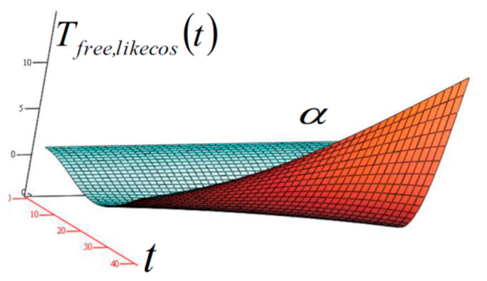
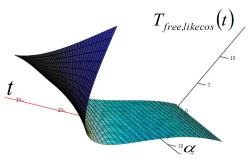
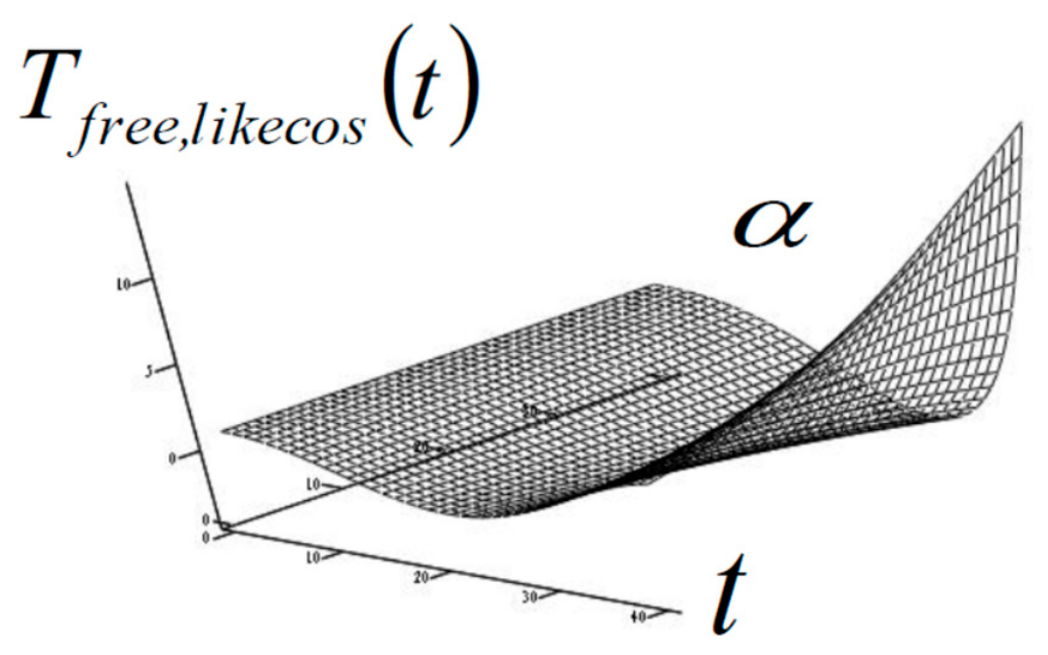
Figure 3, Figure 4 and Figure 5 show the surfaces of the eigen mode of the time functions “like cos”, longitudinal flow of the rheological viscoelastic Maxwell model of a fractional-type material with the property of normal stress relaxation, in a pipe, represented in the coordinate system of the amplitude of the eigen-time mode $T_{free,\mathit{likecos}}\left(t\right)$, time $t$, and exponent $\alpha$ of the fractional-order derivative on the interval $0<\alpha \le 1$. These surfaces are drawn using an approximate analytical expression as follows:$T_{free,\mathit{likecos}}\left(t\right)=T\left(0\right){\displaystyle \sum _{m=1}^{\propto }{\left(-1\right)}^m\frac{1}{k^{2m}}{\displaystyle \sum _{j=1}^{j=m}\frac{E^{-j}}{E_{\alpha }^{m-j}}}}{\displaystyle \frac{t^{-\left[2m+\alpha \left(m-j\right)\right]}}{\Gamma \left(2m+\alpha \left(m-j\right)\right)}}$.

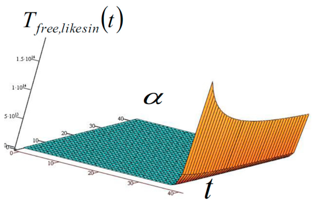
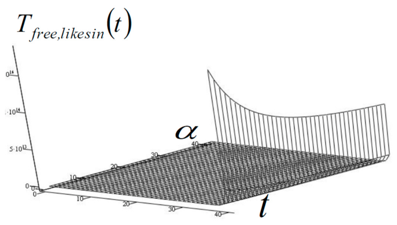
Figure 6 and Figure 7 show the surfaces of the eigen-time functions “likesin”, longitudinal flow of the rheological viscoelastic Maxwell model of a fractional-type material with the property of normal stress relaxation, in a pipe, represented in the coordinate system of the amplitude of the eigen-time mode $T_{free,\mathit{likesin}}\left(t\right)$, time $t$, and exponent $\alpha$ of the fractional-order derivative, on the interval $0<\alpha \le 1$. These surfaces are drawn using an approximate analytical expression $T_{free,\mathit{likecos}}\left(t\right)=T\left(0\right){\displaystyle \sum _{m=1}^{\propto }{\left(-1\right)}^m\frac{1}{k^{2m}}{\displaystyle \sum _{j=1}^{j=m}\frac{E^{-j}}{E_{\alpha }^{m-j}}}}{\displaystyle \frac{t^{-\left[2m+\alpha \left(m-j\right)\right]}}{\Gamma \left(2m+\alpha \left(m-j\right)\right)}}$.

The author notes that Figure 3, Figure 4, Figure 5, Figure 6 and Figure 7 were not included to present numerical data, but rather to illustrate the characteristics of the time series as the differentiation index changes.

8. Discussion

At the suggestion of one of the reviewers, we have included this chapter, which presents contemporary research on fluid flow in pipes. Most contemporary research is focused on engineering tasks and the investigation of flow dynamics in pipes, and is directed towards the oscillations and stability of the pipes themselves or pipe systems, and less on the types of fluids that flow in them and their rheological properties. There is almost no research on the types of material dynamics of different rheological properties.

Wang et al. [20] have come to the following results: A theoretical and numerical model for non-metallic and unbonded flexible pipes was developed based on the nonlinear composite material theory and thick-walled cylindrical theory. The effect of the internal pressure reinforcing layer’s winding scheme on the flexible tube’s mechanical properties is studied, revealing how winding angle changes impact load-bearing performance. The impact of the reinforcing layer’s winding angle on the flexible tube’s ultimate load-bearing performance under internal pressure is examined.

The research focuses on the dynamics of the pipe, and there are no results on the properties of the material flowing through it.

Zhang et al. [21], as aforesaid, arrived at the following results: Key insights into pipes’ bistability under nonlinear resonances are provided; stacking sequence alters superharmonic (subharmonic) amplitude by up to 8% (0.3%); SS thin-walled pipes lack subharmonic bistability for flow speed > 0.1; FGV(FGA) pipe exhibits largest bistable subharmonic(primary) resonance range; FGA(FGV) pipe shows largest bistable response range in lower (higher FORCES). This study explores how graphene nanofillers can be used to control these nonlinear vibrations, providing key insights into the primary and secondary resonance responses of flow-filled graphene-reinforced composite pipes and characterizing their bistable frequency behavior.

In both of these published articles, numerical results and graphic illustrations of the stability of a flowing material (fluid) are useful for engineering practice.

Xiao et al. [22] investigate the complex dynamics of flow and the effects caused by flow.

This paper describes theoretical investigations into the rheological dynamics of oscillating or flowing fractional-type rheological materials using new, original partial differential equations of fractional order. The contours of the rheological material, i.e., the pipes, are considered rigid but of variable cross-section in the longitudinal direction of the rheological material. Considering the research in previous works [20,21,22], we see that the research tasks are completely different and cannot be compared with the studies presented here. The results presented in this work are theoretically analytical, of the fractional type, and completely new. As such, they deserve to become part of a new and completely original scientific monograph. The analyses are based on the obtained eigen-amplitude functions and eigen-time functions of the fractional type, for which we have determined approximate analytical expressions of the eigen and characteristic rheological modes of the fractional type and for rheological oscillations, as well as for rheological creepers. In both cases, there is energy dissipation of the rheological material of the fractional type. The exponent of fractional-order differentiation, which ranges in units from zero to one, affects the degree of fractional-type energy dissipation carried by the rheological material of the Kelvin–Voight or Maxwell material, the dynamics of which are described by the corresponding partial differential equation of the fractional order, in terms of longitudinal displacements or normal stresses in the longitudinal direction. The corresponding ordinary equations of the fractional order in terms of time functions of displacements or time functions of normal stresses in the longitudinal direction for each of the eigen-amplitude functions. For a number of differential equations in terms of eigen-amplitude functions for specifically selected cross-sections and selected boundary conditions in terms of displacements or boundary conditions in terms of normal stresses, we have determined the eigen-amplitude functions.

The comments on the influence of tangential stress due to friction, i.e., the boundary layer effect, are present. However, in this model of longitudinal flow of a rheological Maxwell material of fractional type, a new theoretical approach to the mathematical study of such problems has been opened. The results presented here may serve as a basis for new research into rheological flow dynamics of a fractional type, when the effects of boundary-layer dynamics are also taken into account.

Chapter 12 of the classic Reference [23] and the fundamental monograph on fluid mechanics are devoted to the flow of fluids through pipes of arbitrary shape, with different cross-sections and different resistance to deformation. It contains classical knowledge of fluid mechanics applied to pipe flow. Among the complete contents on fluid mechanics, we also pay attention to References [24,25,26], which were published in the last two decades. The complete field of fluid mechanics is presented in Reference [27].

9. Conclusions

We have presented new scientific analytical results of the theoretical study of the flow (creeping) dynamics of the rheological Maxwell model of a viscoelastic material, fractional type, in a pipe of variable cross-section. Here, we emphasize that, in the study, we neglected the influence of boundary-layer formation on the pipe’s boundary layer using the rheological Maxwell model of a fractional-type viscoelastic material. In particular, we neglected the friction forces at the boundary layer–pipe surface interface. We assumed that this boundary layer is of negligible thickness in relation to the cross-section of the flow stream of the rheological Maxwell model of a viscoelastic material, fractional type, i.e., the cross-section of the pipe, and that these friction forces are negligible in relation to the flow force—the product of the normal stress and the cross-sectional area of the flow stream in each of its cross-sections.

We have presented comparative plots of the surfaces of the eigen and forced fractional forces for the dynamics of oscillation of the rheological Kelvin–Voigt model of an elastophistoviscous material, fractional type, and for the dynamics of flow of the rheological Maxwell model of a viscoelastic material, fractional type. In the structural formula of these two rheological models of materials (Kelvin–Voigt and Maxwell), they contain the same basic rheological elements: Hooke’s ideally elastic element and Newton’s ideally viscous element of fractional type; the former in parallel connection and the latter in series connection; the former is connected with the property of subsequent elasticity (post-elasticity), while the latter is connected with the property of normal stress relaxation.

References

1. Rašković, D.P. Teorija Oscilacija (Theory of Oscillatins), 1st ed.; Naučna Knjiga: Belgrade, Serbia, 1952. [Google Scholar]
2. Rašković, D.P. Teorija Oscilacija (Theory of Oscillatins), 2nd ed.; Naučna Knjiga: Belgrade, Serbia, 1965. [Google Scholar]
3. Rašković, D.P. Teorija Elastičnosti (Theory of Elasticity); Naučna Knjiga: Belgrade, Serbia, 1985. [Google Scholar]
4. Rašković, D.P. Analitička Mehanika (Analytical Mechanics); Mašinski Fakultet Kragujevac: Kragujevac, Serbia, 1974. [Google Scholar]
5. Petrović, M. Elementi Matematičke Fenomenologije (Elements of Mathematical Phenomenology); Srpska Kraljevska Akademija: Belgrade, Serbia, 1911. [Google Scholar]
6. Petrović, M. Fenomenološko Preslikavanje (Phenomenological Mapping); Srpska Kraljevska Akademija: Belgrade, Serbia, 1933; p. 33. (In Serbian) [Google Scholar]
7. Petrović, M. Mecanismes Communs Aux Phenomenes Disparates; Librairie Félix Alcan: Paris, France, 1921. [Google Scholar]
8. Hedrih, K.R. Forced Longitudinal Fractional Type Vibrations of a Rod with Variable Cross Section. In Developments and Novel Approaches in Nonlinear Solid Body Mechanics; Advanced Structured Materials; Abali, B.E., Giorgio, I., Eds.; Springer Nature: Cham, Switzerland, 2020; Chapter 18; pp. 325–344. [Google Scholar] [CrossRef]
9. Hedrih, K.R. An Overview: New Class of Complex Models of Materials Piezoelectric Properties with Differential Constitutive Relation of Fractional Order. Fractal Fract. 2025, 9, 170. [Google Scholar] [CrossRef]
10. Hedrih, K.R. Rheologic Fractional Oscillators or Creepers. Fractal Fract. 2025, 9, 552. [Google Scholar] [CrossRef]
11. Hedrih, R.K.; Milovanović, G.V. Elements of mathematical phenomenology and analogies of electrical and mechanical oscillators of the fractional type with finite number of degrees of freedom of oscillations: Linear and nonlinear modes. Commun. Anal. Mech. 2024, 16, 738–785. [Google Scholar] [CrossRef]
12. Mainardi, F. Fractional Calculus and Waves in Linear Viscoelasticity. In An Introduction to Mathematical Models; Imperial College Press: London, UK, 2010. [Google Scholar] [CrossRef]
13. Kiryakova, V. Generalized Fractional Calculus and Applications. In Pitman Research Notes I Mathematics Series; Longman Scientific & Technical Publisher: Harlow, UK, 1994; p. 301. [Google Scholar]
14. Kilbas, A.A.; Srivastava, H.M.; Trujillo, J.J. Theory and Applications of Fractional Differential Equations; Elsevier: Amsterdam, The Netherlands, 2006. [Google Scholar]
15. Gorenflo, R.; Loutchko, J.; Luchko, Y. Computation of the Mittag-Leffler function and its derivatives. Fract. Calc. Appl. Anal. 2002, 5, 491–518. [Google Scholar]
16. Herrmann, R. Fractional Calculus—An Introduction for Physicists; World Scientific: Singapore, 2014. [Google Scholar] [CrossRef]
17. Mitrinović, D.S.; Djoković, D.Ž. Special Functions (Specijalne Funkcije); Gradjevinska Knjiga: Belgrade, Serbia, 1964; p. 267. [Google Scholar]
18. Rašković, D.P. Tablice Iz Otpornosti Materijala (Tables of Straight of Materials), 11th ed.; Gradflevinska Knjiga: Belgrade, Serbia, 1979. [Google Scholar]
19. Bronstein, I.N.; Semendjajew, K.A. 176 Page in Taschenbuch der Mathenmatik von I.N. Bronstein und K.A. Semendjajew, Mit 427 Abbildungen; B.G. Teubner Verlag Sgesellschaft: Leipzig, Germany, 1958. [Google Scholar]
20. Wang, Y.; Hu, Y.; Zhang, K.; An, W.; Zhou, H.; Lin, Z.; Estefen, S.F. The impact of filament winding configurations on the ultimate load-bearing capacity of non-metallic flexible pipes. Ocean Eng. J. 2025, 341, 122516. [Google Scholar] [CrossRef]
21. Zhang, P.; Li, N.; Tian, H.; Li, J.; Arvin, H. Characterization of bistable frequency responses in nonlinear oscillations of flow-filled graphene-reinforced pipes under various resonances. Eng. Struct. 2026, 353, 122250. [Google Scholar] [CrossRef]
22. Xiao, R.; Su, G.; Zhao, J.; Ye, Z.; Ji, D.; Fan, D. Unsteady Foil Propulsion Over Sediment Beds: Wake Alteration and Efficiency Loss in Particle-Laden Flows. J. Fluid Mech. 2026, 1034, A47. [Google Scholar] [CrossRef]
23. Voronjrc, K.; Obradović, N. Mehanika Fluida (Fluid Mechanics); Gradjevinska Knjiga: Belgrade, Serbia, 1973. [Google Scholar]
24. Tu, J.; Yeoh, G.H.; Liu, C. Computational Fluid Dynamics: A Practical Approach; Elsevier: Amsterdam, The Netherlands, 2012. [Google Scholar]
25. Hrvatska Enciklopedija, Part Fluid, Leksikografski Zavod Miroslav Krleža. 2015. Available online: https://www.enciklopedija.hr/ (accessed on 1 June 2026).
26. Eckert, M. The Dawn of Fluid Dynamics: A Discipline Between Science and Technology; Wiley: Hoboken, NJ, USA, 2006. [Google Scholar]
27. White, F.M. Fluid Mechanics; McGraw-Hill: Columbus, OH, USA, 2011. [Google Scholar]
Figure 1. (a) Structure of the rheological Maxwell basic complex material model, fractional type, which contains, in its structure, a serially connected basic model of Hooke’s ideally elastic element and a basic model of Newton’s ideally viscous fractional-type element. (b,c) Surface of normal stress-surface of normal stress relaxation in the coordinate system: elongation of normal stress relaxation, time, and exponent of differentiation of fractional order.
Fractalfract 10 00471 g001
Figure 2. Element of the rheological Maxwell model of material, fractional type, between two cross-sections in longitudinal coordinates, z 0 . l and z + d z 0 . l , and representations of the axial forces, N z , t = A z σ z , t and N z + d z , t = A z σ z , t + z A z σ z , t d z in those cross-sections.
Fractalfract 10 00471 g002
Figure 3. Surface of the self-eigen-time mode “like cos”, longitudinal flow of the rheological viscoelastic Maxwell model of a fractional-type material in a pipe, presented in the coordinate system of the amplitude of the self-eigen mode T f r e e , likecos t , time t , and exponent α of the fractional-order derivative, on the interval 0 < α 1 .
Fractalfract 10 00471 g003
Figure 4. Surface of the self-eigen-time mode “like cos”, longitudinal flow of the rheological viscoelastic Maxwell model of a fractional-type material in a pipe, presented in the coordinate system of the amplitude of the self-eigen mode T f r e e , likecos t , time t , and exponent α of the fractional-order derivative, on the interval 0 < α 1 , drawings from another direction of visibility.
Fractalfract 10 00471 g004
Figure 5. Surface of the self-eigen-time mode “like cos”, longitudinal flow of the rheological viscoelastic Maxwell model of a fractional-type material in a pipe, presented in the coordinate system of the amplitude of the self-eigen mode T f r e e , likecos t , time t , and exponent α of the fractional-order derivative, on the interval 0 < α 1 , drawings from another direction of visibility and in black and white.
Fractalfract 10 00471 g005
Figure 6. Surface of the self-eigen-time mode “like sin”, longitudinal flow of the rheological viscoelastic Maxwell model of a fractional-type material in a pipe, presented in the coordinate system of the amplitude of the self-eigen mode T f r e e , likesin t of time t and exponent α of the fractional-order derivative, on the interval 0 < α 1 , drawings from another direction of visibility.
Fractalfract 10 00471 g006
Figure 7. Surface of the self-eigen-time mode “like cos”, longitudinal flow of the rheological viscoelastic Maxwell model of a fractional-type material in a pipe, presented in the coordinate system of the amplitude of the self-eigen mode T f r e e , likesin t of time t and exponent α of the fractional-order derivative, on the interval 0 < α 1 , drawings from another direction of visibility and in black and white.
Fractalfract 10 00471 g007
Disclaimer/Publisher’s Note: The statements, opinions and data contained in all publications are solely those of the individual author(s) and contributor(s) and not of MDPI and/or the editor(s). MDPI and/or the editor(s) disclaim responsibility for any injury to people or property resulting from any ideas, methods, instructions or products referred to in the content.