Fractional Texture-Guided and Boundary-Aware Perturbation Learning for Unsupervised Cross-Modality Medical Image Segmentation

Abstract

Unsupervised domain adaptation (UDA) transfers knowledge from a labeled source domain to an unlabeled target domain and is particularly valuable in medical imaging, where dense annotations are costly and acquisition conditions vary. Cross-modality segmentation remains challenging because modality-dependent intensity and texture shifts alter image appearance, while teacher-generated pseudo-labels are often unreliable near anatomical boundaries. We propose a fractional texture-guided and boundary-aware perturbation-learning framework within a student–teacher scheme. On the source side, soft histogram transfer introduces target-related low-order intensity shifts. A multi-order fractional Gram discrepancy between shallow features of the intensity-transferred source and target images then provides a gradient signal for generating magnitude-normalized, range-clipped perturbations. This discrepancy is used as a perturbation cue rather than a direct alignment loss, exposing the student to target-relevant texture and edge-transition variation while preserving source annotations. On the target side, teacher logits are perturbed only within predicted boundary bands to model local contour uncertainty. Box-counting fractal boundary complexity guides the boundary-band width and logit perturbation scale and, together with predictive entropy, regulates pseudo-label supervision. Across five adaptation tasks, the proposed method achieves three-seed mean ± standard deviation Dice scores of 89.24 ± 0.12% and 82.01 ± 0.10% for cardiac MR→CT and CT→MR, 88.65 ± 0.29% and 90.43 ± 0.22% for abdominal MR→CT and CT→MR, and 84.76 ± 0.25% for bSSFP→LGE adaptation. Within the protocol-aware benchmark comparisons, the proposed method attains the highest average Dice score on four of the five tasks and is within 0.07 percentage points of the highest reported value on abdominal CT→MR. Ablation and operator-replacement studies further indicate that the source- and target-side pathways provide complementary benefits. Because all auxiliary perturbation and reliability-weighting modules are used only during adaptation, deployment requires only the adapted segmentation network, without additional inference-time modules or parameters.

1. Introduction

Deep learning has substantially advanced medical image segmentation, but supervised models still rely on dense expert annotations that are costly to obtain. In practice, segmentation models must also contend with distribution shifts: changes in imaging modality, scanner protocol, reconstruction setting, or acquisition site can alter image appearance and degrade performance when a model is deployed outside the training domain. Such shifts are especially pronounced between CT and MR images or across MR sequences, where the same anatomy may present different intensity distributions, contrast patterns, texture characteristics, and boundary sharpness. These domain shifts can be driven by differences in physical imaging parameters, acquisition protocols, and clinical environments [1]. UDA addresses this setting by adapting a model trained with source-domain annotations to unlabeled target-domain data, and its applications in medical image analysis have been broadly reviewed [2].

Early medical UDA methods primarily reduced domain discrepancy through image translation or adversarial feature alignment. For example, target-style generation, denoising-based adaptation, and general adversarial segmentation frameworks have been explored to reduce appearance-level shifts [3,4,5]. Constrained segmentation adaptation, plug-and-play cross-modality adaptation, and synergistic image–feature alignment extended this direction to output-, network-, and feature-level adaptation [6,7,8]. Disentanglement, self-training, and symmetric adaptation further refined alignment-based adaptation [9,10]. Although these approaches can encourage transferable representations, adversarial optimization is often sensitive to training dynamics and may be less stable in medical applications. Consistency regularization and pseudo-label-based learning have therefore become prominent alternatives. These methods derive target-domain supervision from predictions, perturbations, or mixed samples, including cross-domain mixing, prototype-based pseudo-label denoising, semantically guided contrastive learning, and patch-level mixing [11,12,13,14]. They avoid some optimization difficulties associated with adversarial training, but their effectiveness still depends strongly on the quality of target pseudo-labels.

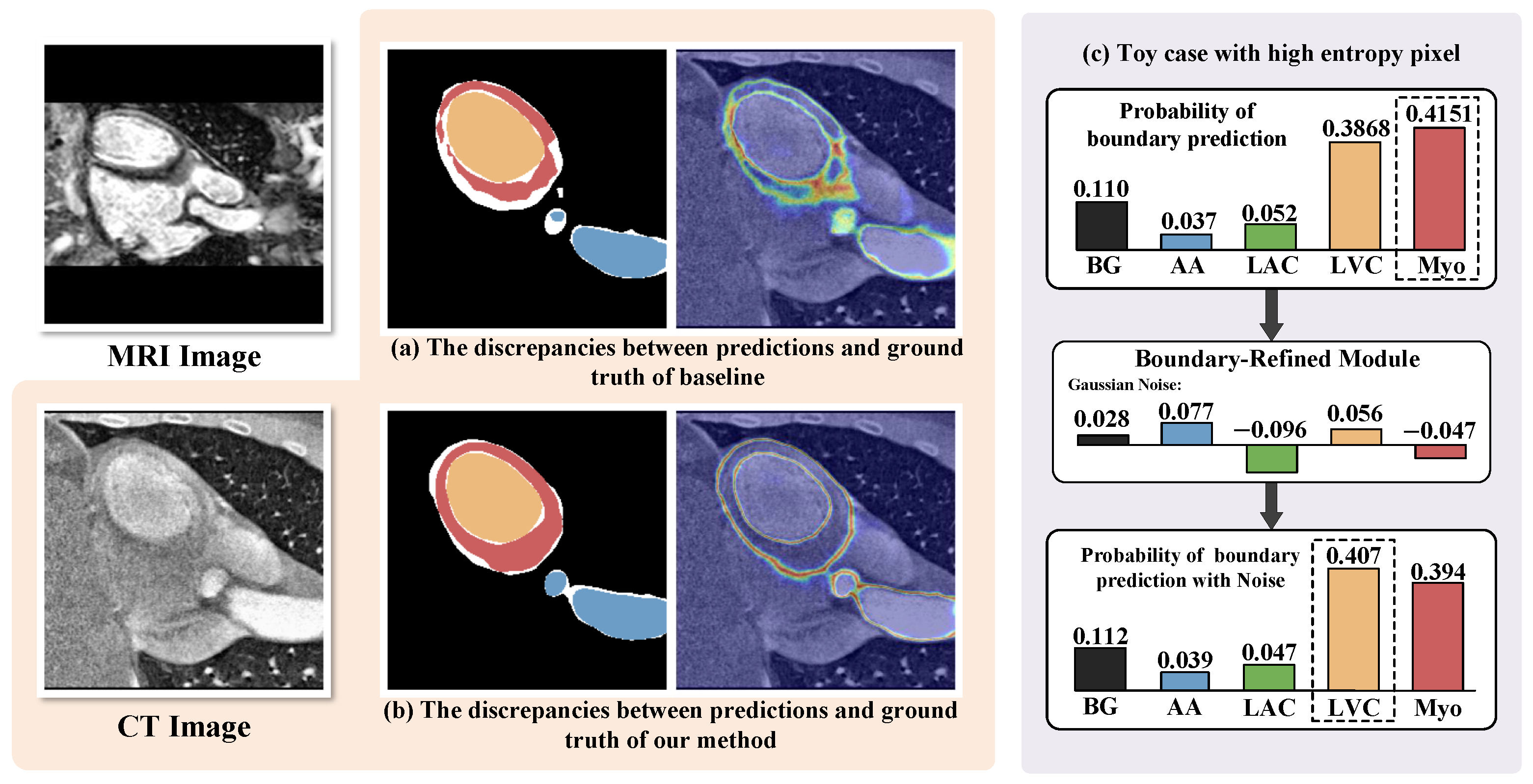
Cross-modality consistency learning faces two related difficulties. First, the appearance gap extends beyond global intensity statistics and includes local contrast, texture, edge transitions, and boundary sharpness; therefore, intensity transfer or generic augmentation alone may leave important modality-specific cues insufficiently modeled. Second, pseudo-label errors are often concentrated near anatomical boundaries, where weak contrast and competing class probabilities make predictions sensitive to small logit changes. Figure 1 illustrates both the concentration of errors around boundaries and the local class instability of a high-entropy pixel. These observations motivate separate but coordinated mechanisms for appearance adaptation and pseudo-label reliability modeling.

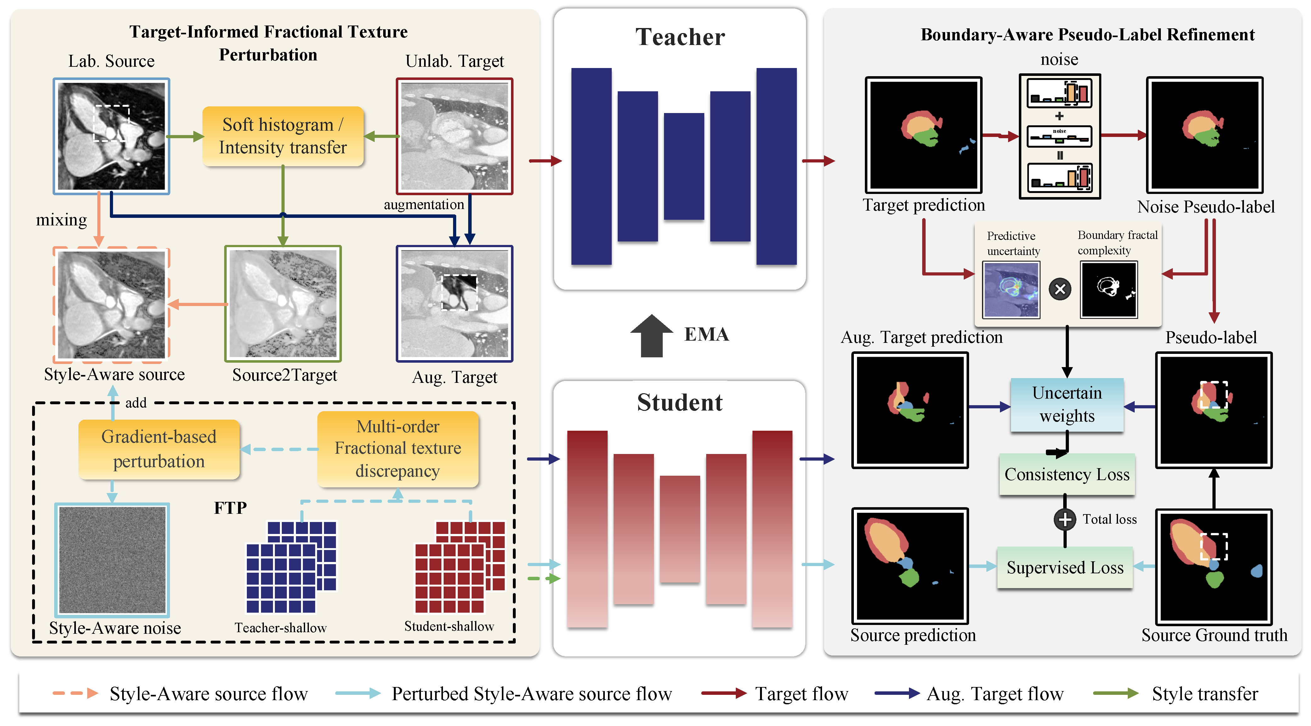
To address these two sources of error, we use two coordinated perturbation-learning pathways. The source branch combines soft histogram transfer with a target-referenced multi-order fractional texture cue to create label-preserving source variants with target-related intensity, texture, and edge-transition variation. The target branch perturbs normalized teacher logits within predicted boundary bands and weights the supervision using predictive entropy and box-counting boundary complexity. Thus, unlabeled target data provide both target-referenced source-appearance variation and reliability-aware boundary supervision.

The main contributions of this work are summarized as follows:

• We formulate cross-modality adaptation as a unified perturbation-learning problem with two complementary objectives: reducing the dependence of source-supervised learning on modality-specific appearance and making target supervision more sensitive to pseudo-label reliability.
• We introduce target-informed fractional texture perturbation. After soft histogram transfer, a batch-level multi-order fractional Gram discrepancy is differentiated with respect to the intensity-transferred source image to generate normalized, range-clipped, label-preserving appearance perturbations for supervised learning.
• We introduce boundary-aware pseudo-label perturbation. Teacher logits are perturbed only within predicted boundary bands to sample local contour alternatives, while predictive entropy and box-counting boundary complexity down-weight unreliable target supervision.
• We evaluate the method on five adaptation tasks from three public benchmarks. The study includes three-seed comparisons, component ablations, analyses of fractional orders and alternative operators, mixing and efficiency studies, within-benchmark robustness checks, and failure-case analysis.

2. Related Work

UDA for medical image segmentation has been studied through several complementary directions, including image translation, feature alignment, semantic alignment, consistency learning, and contrastive learning [2]. A major line of work reduces domain discrepancy by translating source images into a target-like appearance or by aligning latent representations. SASAN and SIFA are representative examples: the former generates target-style images, whereas the latter jointly aligns image and feature spaces in a bidirectional cross-modality framework [3,8]. This alignment-based direction has been further extended through symmetric adaptation, disentanglement with self-training, and semantic similarity constraints [9,10,15]. Other methods introduce category-level, prototype-level, or contrastive objectives to encourage more discriminative cross-domain representations. Category regularization, adaptive semantic alignment, and margin-preserving contrastive learning impose class-aware constraints or preserve semantic separation during adaptation [16,17,18]. Prototype-anchored alignment has also been investigated under source-free assumptions, which differ from the standard source-available UDA setting in terms of source-data access [19]. Although these approaches enrich transferable representations, unpaired source and target slices may still differ not only in modality-dependent appearance but also in slice position, anatomical composition, and foreground proportion.

A complementary line of work learns from unlabeled target images through pseudo-label consistency. Consistency-based methods encourage stable predictions under cross-domain mixing, target-structure learning, semantic contrast, or regional augmentation [11,12,13,14]. Such methods provide dense target-domain training signals without requiring target annotations and can avoid some optimization difficulties associated with adversarial training. However, their effectiveness remains closely tied to the reliability of teacher- or model-generated pseudo-labels. In cross-modality medical image segmentation, pseudo-label errors are often concentrated near anatomical boundaries, where weak contrast, partial-volume effects, and competing class probabilities make predictions sensitive to small perturbations. Therefore, directly treating these boundary pseudo-labels as fully reliable hard supervision may reinforce local contour errors during self-training. Reliability estimation and boundary-aware treatment are consequently important complements to pseudo-label consistency learning.

Recent medical UDA studies have also broadened the adaptation signal beyond conventional adversarial or image-level alignment. Methods based on feature transport, frequency/spatial knowledge distillation, attention-based representations, and dynamic prototype contrastive learning model the domain gap in more structured feature or representation spaces [20,21,22,23]. A further group of recent methods incorporates diffusion-based alignment, masked autoencoding, low-level feature bridging, or text-driven semantic alignment to provide additional generative, structural, or semantic cues for adaptation [24,25,26,27]. Source-free variants operate under different source-data access assumptions [19,28,29]. Foundation-model priors, including SAM- or CLIP-style models, provide another promising direction, but they usually rely on prompting, language-supervision, or model-assumption settings that differ from the source-available UDA protocol studied here [30,31]. Our study remains within the standard source-available UDA setting and focuses on how target-domain appearance variation and predicted-boundary reliability can be incorporated through perturbation learning.

The two mechanisms considered in this work are motivated by complementary fractional and fractal descriptions. Fractional calculus extends integer-order differentiation to non-integer orders, and image-processing studies have shown that fractional responses can preserve sensitivity to gradual intensity transitions while also enhancing local detail [32,33]. This property is useful for describing cross-modality texture and edge-transition differences that are not fully captured by global intensity transfer or a fixed first-order gradient. Fractal analysis, in contrast, characterizes geometric complexity across scales [34,35], and box-counting provides a practical estimator of the fractal dimension of an image [36]. Accordingly, the proposed method uses these two descriptions in different but coordinated roles: fractional texture statistics guide target-referenced source perturbations, whereas box-counting boundary complexity serves as a label-free geometric prior for target pseudo-label reliability. The two branches are integrated through the same consistency-learning pathway, but they address different failure modes: source-side dependence on modality-specific appearance and target-side instability of boundary pseudo-labels.

3. Materials and Methods

3.1. Materials

We evaluate the proposed method on three public, de-identified cross-modality medical image segmentation benchmarks. In every adaptation task, target annotations are withheld from training-time model optimization and pseudo-label generation. These annotations are used for final evaluation, explicitly identified retrospective analyses, and separately reported fully supervised reference models. For cardiac cross-modality segmentation, we use the Multi-Modality Whole Heart Segmentation (MM-WHS) Challenge 2017 dataset [37], which contains 20 unpaired MR volumes and 20 CT volumes with manual annotations. Following the SIFA preprocessing and subject-level split protocol [8], each modality is divided into 16 training volumes and 4 test volumes, and we evaluate both CT→MR and MR→CT adaptation. The foreground structures are the ascending aorta (AA), left-atrium blood cavity (LAC), left-ventricle blood cavity (LVC), and left-ventricular myocardium (MYO). For abdominal multi-organ segmentation, we use 30 CT volumes from the MICCAI multi-atlas abdominal labeling dataset [38] and 20 MR volumes from the ISBI 2019 CHAOS Challenge [39]. Following the subject-level protocol adopted by SIFA [8], the CT domain contains 24 training and 6 test volumes, whereas the MR domain contains 16 training and 4 test volumes. We evaluate CT→MR and MR→CT adaptation for the liver, right kidney, left kidney, and spleen. For multi-sequence cardiac MR adaptation, we use the MS-CMRSeg Challenge dataset [40], which contains late gadolinium enhancement (LGE), balanced steady-state free precession (bSSFP), and T2-weighted sequences from 45 cardiomyopathy patients. Following VarDA [41], we use bSSFP as the labeled source domain and LGE as the unlabeled target domain and retain the released preprocessing and evaluation protocol for comparability. The foreground structures are the LVC, right-ventricular cavity (RVC), and MYO.

3.2. Problem Formulation and Framework Overview

Let ${\mathcal{D}}^s={\left\{(x_i^s,y_i^s)\right\}}_{i=1}^{N_s}$ denote the labeled source-domain dataset, where $x_i^s$ is a source image and $y_i^s$ is its segmentation mask. Let ${\mathcal{D}}^t={\left\{x_i^t\right\}}_{i=1}^{N_t}$ denote the unlabeled target-domain dataset. The goal of unsupervised domain adaptation is to learn a segmentation model that performs well on the target domain without using target annotations during adaptation. We adopt a student–teacher architecture. The student model (${\mathcal{M}}_s$) is optimized by gradient descent, whereas the teacher model (${\mathcal{M}}_t$) is updated as an exponential moving average of the student parameters. The source domain provides reliable pixel-level supervision, and the target domain contributes through teacher-generated pseudo-labels and consistency learning. Figure 2 summarizes two complementary perturbation pathways for cross-modality segmentation. Because unpaired source and target slices can differ in both anatomy and appearance, the source pathway uses target information to form label-preserving source perturbations, while the target pathway perturbs and weights teacher pseudo-labels near predicted boundaries. The student is then trained with source supervision and reliability-aware cross-domain consistency.

3.3. Target-Informed Fractional Texture Perturbation

The source branch uses reliable annotations while reducing dependence on modality-specific appearance. Because unpaired source and target slices can differ in slice position, anatomical content, and foreground proportion, their feature statistics are not treated as directly corresponding observations. Instead of imposing a direct source–target feature-alignment loss, we use target information to generate small, label-preserving appearance perturbations for source images. This keeps the source masks spatially valid while exposing the student to target-related intensity, texture, and edge-transition variations.

We first apply a lightweight differentiable intensity transfer to model low-order appearance differences between modalities. Given a source image ($x^s$) and an unpaired target image ($x^t$), both normalized to $[0,1]$, and we define $B_h$ histogram bins with centers expressed as ${\left\{c_b\right\}}_{b=1}^{B_h}$. The bin centers are uniformly spaced over the normalized intensity range, and we set $B_h=256$ in all experiments. For a given pixel intensity (u), its soft assignment to the b-th bin, the soft histogram, and the corresponding cumulative distribution function (CDF) are defined as

$${\omega }_b\left(u\right)={\displaystyle \frac{exp\left(-\frac{{(u-c_b)}^2}{2{\sigma }_h^2}\right)}{{\sum }_{r=1}^{B_h}exp\left(-\frac{{(u-c_r)}^2}{2{\sigma }_h^2}\right)}},H_x\left(b\right)={\displaystyle \frac{1}{|\Omega |}}\sum _{p\in \Omega }{\omega }_b\left(x\left(p\right)\right),C_x\left(b\right)={\displaystyle \sum _{r=1}^b}{H}_x\left(r\right),$$

(1)

where $\Omega$ denotes the image lattice and ${\sigma }_h$ controls the smoothness of the soft-bin assignment. A differentiable source-to-target CDF mapping is obtained by softly matching cumulative probabilities. For source bin b and target bin r, we define

$${\alpha }_{br}^{s\to t}={\displaystyle \frac{exp\left(-|C_{x^s}\left(b\right)-C_{x^t}\left(r\right)|/{\tau }_h\right)}{{\sum }_{\ell =1}^{B_h}exp\left(-|C_{x^s}\left(b\right)-C_{x^t}(\ell )|/{\tau }_h\right)}},{\Pi }_{s\to t}\left(b\right)={\displaystyle \sum _{r=1}^{B_h}}{\alpha }_{br}^{s\to t}{c}_r.$$

(2)

The intensity-transferred source image is then computed as

$$x_{\mathrm{sty}}^s\left(p\right)=(1-\rho )x^s\left(p\right)+\rho {\displaystyle \sum _{b=1}^{B_h}}{\omega }_b\left(x^s\left(p\right)\right){\Pi }_{s\to t}\left(b\right),\rho \sim \mathcal{U}(0,1).$$

(3)

Here, ${\tau }_h$ controls the softness of CDF matching, and $\rho$ determines the interpolation strength between the original and mapped intensities. Because this operation changes image intensities without spatial warping, the original source mask remains aligned with the transformed image and can be retained for supervision.

Intensity transfer mainly captures low-order intensity shifts. To further model target-relevant texture and boundary-transition variations, we introduce multi-order fractional texture statistics. Let ${\varphi }_s^{\ell }(·)$ and ${\varphi }_t^{\ell }(·)$ denote shallow feature extractors from the student and teacher models, respectively. For the intensity-transferred source image ($x_{\mathrm{sty}}^s$) and the target image ($x^t$), we extract

$$F_{\mathrm{sty}}^s={\varphi }_s^{\ell }\left(x_{\mathrm{sty}}^s\right),F^t=\mathrm{sg}\left({\varphi }_t^{\ell }\left(x^t\right)\right),$$

(4)

where $\mathrm{sg}(·)$ denotes the stop-gradient operation. The target feature extracted by the teacher provides a stable target-domain reference, while gradients for perturbation generation are propagated only through the student source branch.

For a fractional order ($\nu$), we compute truncated Grünwald–Letnikov finite differences along the horizontal and vertical directions:

$$\begin{array}{c}{\left(D_x^{\nu }F\right)}_{c,i,j}={\displaystyle \sum _{m=0}^K}{g}_m^{\nu }{F}_{c,i,j-m},{\left(D_y^{\nu }F\right)}_{c,i,j}={\displaystyle \sum _{m=0}^K}{g}_m^{\nu }{F}_{c,i-m,j},\\ T^{\nu }\left(F\right)=\sqrt{{\left(D_x^{\nu }F\right)}^2+{\left(D_y^{\nu }F\right)}^2+ϵ}.\end{array}$$

(5)

Here, K is the truncation length, $ϵ$ is a numerical stability constant, and $g_m^{\nu }={(-1)}^m\left({\displaystyle \genfrac{}{}{0pt}{}{\nu }{m}}\right)$ with $\left({\displaystyle \genfrac{}{}{0pt}{}{\nu }{m}}\right)={\displaystyle \frac{\Gamma (\nu +1)}{\Gamma (m+1)\Gamma (\nu -m+1)}}$. The finite differences are applied channel-wise to the shallow feature map. Different fractional orders characterize complementary local appearance patterns. In this work, we use the compact order set expressed as $\mathcal{V}=\{0.7,1.0,1.3\}$, which is centered on the standard first-order derivative and spans smoother transitions, standard gradient responses, and sharper local texture changes. The contributions of individual and combined orders are evaluated in Section 4.3. For each fractional order, we compute the Gram statistic of the fractional texture response by flattening the spatial dimensions:

$$G_{\nu }\left(F\right)={\displaystyle \frac{1}{HW}}{\tilde{T}}^{\nu }\left(F\right){\tilde{T}}^{\nu }{\left(F\right)}^{\top },$$

(6)

where ${\tilde{T}}^{\nu }\left(F\right)$ denotes the matrix obtained by reshaping $T^{\nu }\left(F\right)$ into a channels-by-spatial positions matrix. Here, H and W denote the height and width of the shallow feature map, and ${\parallel ·\parallel }_F$ is the Frobenius norm used below. The batch-level source–target fractional texture discrepancy is defined as

$${\mathcal{D}}_{\mathrm{frac}}={\displaystyle \frac{1}{\left|\mathcal{V}\right|}}\sum _{\nu \in \mathcal{V}}{∥{\displaystyle \frac{1}{B_s}}{\displaystyle \sum _{i=1}^{B_s}}{G}_{\nu }\left(F_{\mathrm{sty},i}^s\right)-{\displaystyle \frac{1}{B_t}}{\displaystyle \sum _{j=1}^{B_t}}{G}_{\nu }\left(F_j^t\right)∥}_F^2,$$

(7)

where $B_s$ and $B_t$ denote the source and target batch sizes, respectively.

The batch averages summarize domain-level texture statistics without requiring one-to-one anatomical pairing between source and target images. Importantly, ${\mathcal{D}}_{\mathrm{frac}}$ is used only to generate a source perturbation. It is not added to the segmentation objective as a feature-alignment loss, and no model parameters are updated directly using ${\mathcal{D}}_{\mathrm{frac}}$. Instead, its computational graph is differentiated with respect to the intensity-transferred source image to obtain a target-referenced perturbation direction. Specifically, we construct

$$\begin{array}{c}{g}_{\mathrm{frac}}={\nabla }_{x_{\mathrm{sty}}^s}{\mathcal{D}}_{\mathrm{frac}},{\Delta }_{\mathrm{frac}}=-{ϵ}_{\mathrm{frac}}{\displaystyle \frac{g_{\mathrm{frac}}}{\mathrm{mean}\left(\right|g_{\mathrm{frac}}\left|\right)+ϵ}},\\ x_{\mathrm{ftp}}^s=\mathrm{clip}\left(x_{\mathrm{sty}}^s+\mathrm{sg}\left({\Delta }_{\mathrm{frac}}\right),0,1\right).\end{array}$$

(8)

Here, ${ϵ}_{\mathrm{frac}}$ controls the average perturbation magnitude after gradient normalization. The negative gradient direction corresponds to a first-order step that reduces the target-referenced fractional texture discrepancy. The stop-gradient operation prevents second-order optimization through the perturbation generation process. Because the perturbation is magnitude-normalized and clipped to the valid intensity range and does not deform the image spatially, the source mask ($y^s$) remains aligned with $x_{\mathrm{ftp}}^s$ and is reused for supervision. The supervised source loss is computed as

$${\mathcal{L}}_{\sup }={\mathcal{L}}_{\mathrm{CE}}\left({\mathcal{M}}_s\left(x_{\mathrm{ftp}}^s\right),y^s\right)+{\mathcal{L}}_{\mathrm{Dice}}\left({\mathcal{M}}_s\left(x_{\mathrm{ftp}}^s\right),y^s\right).$$

(9)

Through this design, the student learns from reliable source annotations while being exposed to target-informed intensity, texture, and boundary-transition variations, reducing its dependence on source-specific appearance cues.

3.4. Boundary-Aware Pseudo-Label Perturbation

Teacher-generated pseudo-labels provide dense target-domain supervision, but their reliability is spatially nonuniform. Boundary pixels are particularly sensitive because small changes in logits may change the predicted class. We therefore perturb normalized teacher logits only within pseudo-label boundary bands and use the resulting labels as stochastic consistency targets. This operation models local contour uncertainty and reduces the risk that the student overfits to a single unstable teacher boundary. Predictive entropy and boundary complexity then regulate the strength of pseudo-label supervision so that stable regions contribute more strongly than uncertain or geometrically irregular boundaries. We refer to the complete target-side procedure as boundary-aware pseudo-label perturbation (BAPLP). For a target image ($x^t$), the teacher model produces logits ($Z^t$), a probability map ($P^t$), and an initial pseudo-label (${\widehat{y}}^t$):

$$Z^t={\mathcal{M}}_t\left(x^t\right),P^t=\mathrm{softmax}\left(Z^t\right),{\widehat{y}}^t=arg\underset{c\in \{0,\dots ,C-1\}}{max}{P}^{t,c}.$$

(10)

Here, C is the number of classes, and the background class is indexed by $c=0$. Based on the initial pseudo-label, we extract a boundary band for each foreground class using morphological dilation and erosion, then merge all foreground boundaries:

$$B_0=B\left(n_0\right)={\displaystyle \underset{c=1}{\overset{C-1}{\bigvee }}}\left[\mathrm{Dilate}\left(\mathbb{I}[{\widehat{y}}^t=c],n_0\right)-\mathrm{Erode}\left(\mathbb{I}[{\widehat{y}}^t=c],n_0\right)\right],$$

(11)

where $\mathbb{I}[·]$ is the indicator function, ⋁ denotes the logical union over foreground classes, and $n_0$ is the morphological radius used to form the initial boundary band. We set $n_0=1$. The resulting mask ($B_0$) identifies regions in which the teacher prediction is most likely to be sensitive to local boundary perturbations.

To quantify the geometric irregularity of the pseudo-label boundary, we estimate its box-counting fractal dimension (FD). Given a set of box sizes ($\mathcal{R}=\{r_1,r_2,\dots ,r_L\}$), let $N_r\left(B_0\right)$ denote the number of boxes with a side length (r) that intersects the boundary mask ($B_0$). In implementation, $\mathcal{R}$ consists of valid powers of two that fit within the shorter side of the boundary mask, and the same rule is used for all datasets. The fractal dimension is estimated from the slope of the log–log relation between the box size and the number of occupied boxes:

$$\begin{array}{c}{D}_f\left(B_0\right)=-{\displaystyle \frac{{\sum }_{r\in \mathcal{R}}(a_r-\overline{a})(b_r-\overline{b})}{{\sum }_{r\in \mathcal{R}}{(a_r-\overline{a})}^2+ϵ}},a_r=logr,b_r=log(N_r\left(B_0\right)+ϵ),\\ {\tilde{D}}_f=\mathrm{clip}\left({\displaystyle \frac{D_f\left(B_0\right)-D_{min}}{D_{max}-D_{min}+ϵ}},0,1\right).\end{array}$$

(12)

Here, $D_f\left(B_0\right)$ measures the multi-scale geometric complexity of the pseudo-label boundary, and ${\tilde{D}}_f$ is the corresponding normalized complexity score. We set $D_{min}=0.5$ and $D_{max}=1.5$ and clip ${\tilde{D}}_f$ to $[0,1]$ to limit the influence of empty or highly fragmented boundary masks. A larger normalized FD is treated as a cue for more conservative boundary supervision rather than as a calibrated probability of pseudo-label error.

The normalized boundary complexity determines both the discrete boundary-band radius and the continuous logit-noise scale:

$$\begin{array}{c}{n}_f={\mathrm{clip}}_{[n_{min},n_{max}]}\left(\mathrm{round}\left[n_{min}+(n_{max}-n_{min}){\tilde{D}}_f\right]\right),\\ {\sigma }_f={\sigma }_{min}+({\sigma }_{max}-{\sigma }_{min}){\tilde{D}}_f.\end{array}$$

(13)

Here, $\mathrm{round}(·)$ maps the radius to the nearest integer, and ${\mathrm{clip}}_{[n_{min},n_{max}]}(·)$ constrains it to the valid radius range. Thus, $n_f$ is an integer-valued morphological radius, whereas ${\sigma }_f$ varies continuously within $[{\sigma }_{min},{\sigma }_{max}]$. More irregular pseudo-label boundaries receive a wider local perturbation band and a larger logit-noise scale. The adaptive boundary mask is then recomputed as $B_f=B\left(n_f\right)$. Before perturbation, the teacher logits are normalized to reduce sample-wise scale variation:

$${\overline{Z}}^t={\displaystyle \frac{Z^t-\mu \left(Z^t\right)}{\sigma \left(Z^t\right)+ϵ}}.$$

(14)

Here, $\mu \left(Z^t\right)$ and $\sigma \left(Z^t\right)$ are computed over all class and spatial entries of the current target sample. Because the same scalar shift and positive scale are applied to every class logit in that sample, normalization preserves the pre-perturbation argmax while making the subsequent noise scale more comparable across samples. Boundary logit perturbation is performed only inside the adaptive boundary band:

$$Z_{\mathrm{bp}}^t={\overline{Z}}^t+\Xi \odot B_f,\Xi \sim \mathcal{N}(0,{\sigma }_f^2),{\widehat{y}}_{\mathrm{bp}}^t=arg\underset{c\in \{0,\dots ,C-1\}}{max}\mathrm{softmax}{\left(Z_{\mathrm{bp}}^t\right)}^c.$$

(15)

Here, the entries of $\Xi$ are sampled independently, $\Xi$ has the same shape as $Z^t$, and the spatial mask ($B_f$) is broadcast along the class dimension. The perturbed pseudo-label ${\widehat{y}}_{\mathrm{bp}}^t$ is interpreted as a local boundary alternative around the teacher prediction, not as a corrected label that is assumed to be more accurate.

Finally, we assign an adaptive weight to each target pixel to control the strength of pseudo-label supervision. The predictive entropy at pixel k is computed from the original teacher probability map ($P^t$):

$$H_k=-{\displaystyle \sum _{c=0}^{C-1}}{P}_k^{t,c}log{P}_k^{t,c},{\overline{H}}^{\left(q\right)}=\beta {\overline{H}}^{(q-1)}+(1-\beta ){\displaystyle \frac{1}{|\Omega |}}\sum _{k\in \Omega }{H}_k,$$

(16)

where ${\overline{H}}^{\left(q\right)}$ is an EMA estimate of the mean target entropy at iteration q and $\beta$ is the EMA coefficient. The final target weight combines an entropy-aware term and a fractal-complexity-aware term:

$$w_k^t=w_k^{\mathrm{ent}}{w}_k^{\mathrm{fra}},w_k^{\mathrm{ent}}=\left\{\begin{array}{cc}1,\hfill & H_k\le \overline{H},\hfill \\ exp\left(-{\displaystyle \frac{{(H_k-\overline{H})}^2}{2{\sigma }_w^2}}\right),\hfill & H_k>\overline{H},\hfill \end{array}\right.w_k^{\mathrm{fra}}=exp(-\eta {\tilde{D}}_f{B}_{f,k}).$$

(17)

Here, $\overline{H}$ denotes the current EMA estimate (${\overline{H}}^{\left(q\right)}$), and $\eta$ controls the strength of fractal-complexity-based down-weighting within the boundary band. The entropy-aware term down-weights locally uncertain predictions, while the fractal-complexity-aware term further reduces the contribution of pixels inside the boundary band when the predicted boundary has higher overall geometric complexity. Consequently, stable interior regions provide stronger pseudo-label supervision, whereas high-entropy or geometrically irregular boundary regions contribute less to the training objective.

3.5. Cross-Domain Consistency and Optimization

The source and target pathways are integrated through cross-domain mixed-sample consistency. Each mixed image contains regions supervised by source ground truth and regions supervised by reliability-weighted target pseudo-labels. Given a binary mixing mask ($\mathbf{M}$), ${\mathbf{M}}_k=1$ indicates that pixel k is taken from the target image, and ${\mathbf{M}}_k=0$ indicates that it is taken from the source image. We use a random rectangular patch mask by default and construct the mixed image, label map, and weight map as

$$\begin{array}{c}{x}_{\mathrm{mix}}=\mathbf{M}\odot x^t+(1-\mathbf{M})\odot x_{\mathrm{ftp}}^s,\\ y_{\mathrm{mix}}=\mathbf{M}\odot {\widehat{y}}_{\mathrm{bp}}^t+(1-\mathbf{M})\odot y^s,\\ w_{\mathrm{mix},k}={\mathbf{M}}_k{w}_k^t+(1-{\mathbf{M}}_k).\end{array}$$

(18)

Here, ⊙ denotes element-wise multiplication. Because $\mathbf{M}$ is binary, $y_{\mathrm{mix}}$ remains an integer-valued class map; one-hot expansion is applied only when evaluating Equation (19). Source regions are supervised by ground-truth labels with full confidence, whereas target regions are supervised by teacher-generated pseudo-labels with the adaptive weight ($w_k^t$). This design allows reliable target pixels to contribute useful supervision while preventing uncertain or geometrically complex boundary pixels from dominating the optimization.

The student prediction based onthe mixed image is denoted as $P_{\mathrm{mix}}=\mathrm{softmax}\left({\mathcal{M}}_s\left(x_{\mathrm{mix}}\right)\right)$. We compute the weighted pixel-wise consistency loss as

$${\mathcal{L}}_{\mathrm{cons}}=-{\displaystyle \frac{1}{|\Omega |}}\sum _{k\in \Omega }{w}_{\mathrm{mix},k}{\displaystyle \sum _{c=0}^{C-1}}\mathbb{I}[y_{\mathrm{mix},k}=c]log{P}_{\mathrm{mix},k}^c,$$

(19)

where $\Omega$ is the image lattice, C is the number of classes, and $\mathbb{I}[·]$ is the indicator function. This loss encourages the student model to produce consistent predictions based on cross-domain mixed samples while respecting the different reliability levels of source and target supervision. The overall objective combines the supervised source loss and the weighted cross-domain consistency loss:

$${\mathcal{L}}_{\mathrm{total}}={\mathcal{L}}_{\sup }+{\lambda }_u\left(q\right){\mathcal{L}}_{\mathrm{cons}},{\lambda }_u\left(q\right)={\lambda }_u^{max}exp\left[-5{\left(1-min\left({\displaystyle \frac{q}{Q}},1\right)\right)}^2\right],$$

(20)

where q denotes the training iteration, Q is the ramp-up length, and ${\lambda }_u^{max}$ is the maximum consistency weight. The ramp-up strategy is used because target pseudo-labels are usually less reliable during the early stages of training. Their influence is gradually increased as the teacher model becomes more stable. Accordingly, ${\mathcal{D}}_{\mathrm{frac}}$ influences training only through the generated source images and does not appear as a separate alignment term in the final objective. After each student update, the teacher model is updated by EMA:

$${\Theta }_t^{(q+1)}=\gamma {\Theta }_t^{\left(q\right)}+(1-\gamma ){\Theta }_s^{(q+1)},$$

(21)

where ${\Theta }_s$ and ${\Theta }_t$ denote the parameters of the student and teacher models, respectively, and $\gamma$ is the EMA decay coefficient. During training, no target-domain labels are used for model optimization. Unless otherwise specified, the fractional-order set is fixed as $\mathcal{V}=\{0.7,1.0,1.3\}$, and the same hyperparameter settings are used across adaptation tasks to maintain a common configuration.

4. Results

4.1. Implementation Details and Evaluation Metrics

The proposed method is implemented in PyTorch 1.13.1 and trained on a single NVIDIA Tesla A30 GPU. Following common practice in medical UDA segmentation, all experiments are conducted in a 2D slice-wise training setting. We adopt ResNet-50 as the backbone and use DeepLab-v2 as the segmentation network. The student and teacher models share the same architecture. During training, the student model is optimized by back-propagation, while the teacher model is updated as an exponential moving average of the student parameters. Gradients are not propagated through the teacher branch. During inference, only the adapted segmentation network is retained; perturbation generation, boundary weighting, and teacher-side operations are discarded. For MM-WHS and the Abdominal Multi-Organ dataset, we follow the SIFA preprocessing pipeline and fixed subject-level 80/20 splits. For MS-CMRSeg, we follow the released VarDA preprocessing and bSSFP→LGE adaptation protocol. The bidirectional tasks use the same fixed, domain-specific splits by exchanging source and target roles. During adaptation, target annotations are withheld from pseudo-label generation, hyper-parameter tuning, and model selection. They are used only for final evaluation, explicitly identified retrospective analyses, and the separately reported fully supervised reference rows. The principal benchmark tables report the mean ± standard sample deviation over three runs with 666, 777, and 888 seeds.

Table 1. Main optimization and module settings used in the proposed framework. The default values are retained across adaptation tasks unless otherwise specified. Target annotations are not used for adaptation, hyper-parameter tuning, or model selection.

Category	Hyperparameter	Value
Network andtraining	Backbone/segmentation head	ResNet-50/DeepLab-v2
	Optimizer/momentum/weight decay	SGD/0.9/${10}^{-5}$
	Learning rate, backbone/head	$0.001$/$0.01$
	Source/target batch size; iterations	$B_s=2$, $B_t=2$; 50,000
	Teacher EMA decay $\gamma$	0.99
Soft histogramtransfer	Number of bins ($B_h$)	256
	Bin bandwidth/CDF temperature	${\sigma }_h=0.02$, ${\tau }_h=0.05$
	Intensity interpolation coefficient	$\rho \sim \mathcal{U}(0,1)$
Fractional textureperturbation	Order set ($\mathcal{V}$)	$\{0.7,1.0,1.3\}$
	Perturbation magnitude (${ϵ}_{\mathrm{frac}}$)	0.02
	GL truncation length/numerical stabilizer	$K=5$, $ϵ={10}^{-6}$
Boundary-awaretarget learning	Initial/minimum/maximum radius	$n_0=1$, $n_{min}=1$, $n_{max}=3$
	Boundary logit-noise scale	${\sigma }_{min}=0.05$, ${\sigma }_{max}=0.30$
	Fractal normalization interval	$D_{min}=0.5$, $D_{max}=1.5$
	Entropy bandwidth/EMA coefficient	${\sigma }_w=0.2$, $\beta =0.99$
	Fractal down-weighting coefficient	$\eta =0.4$
Cross-domainconsistency	Maximum weight/ramp-up length	${\lambda }_u^{max}=1.0$, $Q=10,000$
	Mixing strategy	Patch-based mixing

summarizes the default optimization and module settings used across adaptation tasks. These settings cover network, optimization, soft histogram transfer, fractional texture perturbation, boundary-aware target learning, and cross-domain consistency. All perturbation and reliability-weighting operations are removed after adaptation, and deployment retains only the adapted segmentation network.

The principal benchmark comparisons report Dice valuesand the average symmetric surface distance (ASD), which are the metrics most consistently available in the compared UDA literature. Additional component, sensitivity operator-replacement, and robustness analyses also report HD95, BF1@2, and surface Dice values at one-, two-, and three-voxel tolerances. Because reliable physical-spacing metadata are not consistently available for the stored preprocessed arrays used in these additional analyses, these tolerance-based boundary metrics are reported on the preprocessed voxel grid. Class-wise scores are averaged over foreground structures. The Dice metric, BF1, and surface Dice valuesare reported as percentages; ASD and HD95 are distance-based metrics. Higher values for the Dice metric, BF1, and the surface Dice metricand lower values for ASD and HD95, indicate better segmentation quality.

4.2. Comparison with Representative UDA Methods

We compare the proposed method with representative medical UDA methods whose results are available under matched or closely corresponding benchmark settings. The comparison includes adversarial or image-translation methods [8,42]; consistency-, semantically, contrast-, and pseudo-label-based methods [11,15,17,18,41,43,44,45]; frequency-, transport-, or probabilistic methods [20,21]; and recent Transformer, diffusion, masked modeling, and low-level cue approaches [22,23,24,25,26,27]. The w/o adaptation and fully supervised rows are source-only and target-labeled references, respectively; the latter is not a UDA baseline. A dagger denotes results reproduced in our environment, while unmarked entries are values reported in the cited papers. Missing metrics are excluded from column-wise ranking. Because protocols, backbones, training budgets, source-data access, and validation settings may differ, the overall ranking across published methods should be interpreted as a descriptive benchmark comparison. Therefore, paired statistical tests were applied only to the dagger-marked baselines reproduced in our environment, for which matched volume-level results were available. For each reproduced baseline, we conducted paired t-tests comparing its volume-level average Dice scores with the corresponding scores from the proposed method across the three seeds. Methods reported only as aggregate literature results were not included in these tests because their per-volume predictions or scores are unavailable. Statistical significance was defined as $p<0.05$. For the proposed method,

Table 2. Protocol-aware comparison on MM-WHS: Daggered entries are reproduced; other values are from cited papers. Ours is mean ± standard sample deviation over three seeds. Dashes denote unreported metrics; bold and underlined values mark the best and second-best UDA entries after excluding reference rows.

Method		Dice (%) ↑					ASD ↓
		AA	LAC	LVC	MYO	Average	AA	LAC	LVC	MYO	Average
Cardiac MR → CT	Supervised training	88.93	92.27	93.09	88.10	90.60	1.60	2.02	1.55	1.57	1.69
	w/o adaptation	32.24	65.79	10.29	5.81	28.53	11.56	7.44	11.78	22.65	13.35
	AdvEnt † [42]	83.48	82.20	77.88	54.20	74.44	7.26	5.72	3.98	4.34	5.32
	SIFA † [8]	81.32	79.55	73.76	61.57	74.05	7.86	6.15	5.54	8.48	7.01
	DACS † [11]	84.79	85.07	80.17	69.48	79.88	9.93	5.55	4.93	4.02	6.11
	SSC [15]	82.00	85.30	88.40	67.60	80.80	6.20	4.10	3.00	3.40	4.20
	SE_ASA [17]	83.80	85.20	82.90	71.70	80.90	9.60	4.20	3.90	3.90	5.40
	MPSCL† [18]	87.75	88.24	85.98	70.11	83.02	7.63	2.77	2.71	3.43	4.13
	PUFT [20]	88.10	88.50	87.50	74.10	84.60	2.30	2.60	3.40	3.30	2.90
	MA-UDA [22]	90.80	88.70	77.60	67.40	81.10	5.70	3.80	7.60	5.20	5.60
	DPCL [23]	90.00	88.70	88.20	74.50	85.40	6.60	4.10	4.40	3.70	4.70
	MAPSeg [25]	93.30	87.30	89.10	78.90	87.10	–	–	–	–	–
	LowBridge-UNet [26]	94.00	88.00	85.10	78.60	86.40	–	–	–	–	4.10
	TCSA-UDA [27]	82.50	87.10	85.70	74.30	82.40	13.20	7.20	3.50	3.60	6.90
	Prior FSUDA [46]	86.80	87.50	84.60	82.40	85.30	1.60	2.50	3.20	3.10	2.60
	FSUDA [21]	88.20	88.90	85.20	82.20	86.10	1.50	2.60	2.50	2.90	2.40
	Ours	94.38 ± 0.26	91.73 ± 0.56	90.02 ± 0.76	80.84 ± 0.59	89.24 ± 0.12	1.48 ± 0.35	2.35 ± 0.28	1.78 ± 0.05	2.33 ± 0.10	1.99 ± 0.10
Cardiac CT → MR	Supervised training	82.37	86.63	91.81	80.14	85.24	3.61	2.21	2.58	1.77	2.54
	w/o adaptation	5.26	4.54	54.94	7.78	18.13	24.95	15.42	9.30	7.56	14.31
	AdvEnt † [42]	54.37	63.49	76.67	41.48	59.00	6.67	3.92	4.01	4.83	4.86
	SIFA † [8]	65.29	62.27	78.90	47.27	63.43	7.32	7.43	3.82	4.43	5.75
	DACS † [11]	60.64	38.05	78.09	66.46	60.81	7.43	13.88	6.33	3.77	7.85
	SE_ASA [17]	68.30	74.60	81.00	55.90	69.90	4.90	3.60	5.40	3.20	4.30
	MPSCL † [18]	63.93	75.07	76.58	50.34	66.48	5.65	2.88	4.35	3.96	4.21
	PUFT [20]	69.30	77.40	83.00	63.60	73.30	4.80	3.60	2.90	3.10	3.60
	MA-UDA [22]	71.00	67.40	77.50	59.10	68.70	4.40	6.90	5.60	4.20	5.30
	DPCL [23]	70.30	77.00	82.90	53.60	71.00	5.00	2.90	3.20	4.60	3.90
	MAPSeg [25]	78.50	81.80	92.10	68.80	80.30	–	–	–	–	–
	LowBridge-UNet [26]	62.70	62.30	88.30	63.40	69.20	–	–	–	–	5.90
	TCSA-UDA [27]	69.00	74.90	83.50	59.20	71.60	5.30	4.50	5.70	5.00	5.10
	Prior FSUDA [46]	62.40	72.10	81.20	66.50	70.60	4.90	4.50	3.00	3.80	4.10
	FSUDA [21]	72.50	78.60	82.60	68.40	75.50	4.70	3.60	2.50	2.40	3.30
	Ours	82.10 ± 1.70	81.20 ± 1.54	92.06 ± 0.29	72.69 ± 1.16	82.01 ± 0.10	3.52 ± 0.81	2.42 ± 0.36	1.69 ± 0.20	1.88 ± 0.16	2.35 ± 0.17

,

Table 3. Protocol-aware comparison on the Abdominal Multi-Organ dataset. Daggered entries are reproduced; other values are from cited papers. Ours is mean ± standard sample deviation over three seeds. Dashes denote unreported metrics; bold and underlined values mark the best and second-best UDA entries after excluding reference rows.

Method		Dice (%) ↑					ASD ↓
		Liver	R.Kidney	L.Kidney	Spleen	Average	Liver	R.Kidney	L.Kidney	Spleen	Average
Abdomen MR → CT	Supervised training	92.14	88.06	87.91	89.07	89.30	1.22	0.80	1.06	0.68	0.94
	w/o adaptation	75.13	41.39	55.33	55.62	56.87	3.22	8.69	9.35	6.37	8.99
	AdvEnt † [42]	83.07	82.95	81.51	82.70	82.56	2.83	1.24	1.30	1.08	1.61
	SIFA † [8]	85.08	82.53	84.34	83.55	83.88	2.54	1.27	1.40	1.08	1.57
	DACS † [11]	88.65	74.90	70.19	71.86	76.40	1.85	1.75	1.88	2.02	1.87
	SSC [15]	88.50	83.30	82.00	83.10	84.20	1.30	1.00	1.20	1.60	1.30
	MPSCL † [18]	88.85	82.41	83.82	83.18	84.57	1.01	1.45	1.38	2.68	1.63
	PUFT [20]	89.70	84.90	87.60	86.30	87.30	1.40	1.10	1.50	1.80	1.50
	Diffusion DA [24]	89.00	85.60	85.60	85.80	86.50	1.50	1.30	1.20	1.20	1.30
	TCSA-UDA [27]	88.43	83.72	80.35	81.15	83.41	0.52	0.64	0.79	0.88	0.71
	Prior FSUDA [46]	88.60	83.50	81.70	83.50	84.30	1.40	1.10	1.20	1.60	1.30
	FSUDA [21]	89.80	85.40	87.90	88.40	87.80	1.20	1.00	1.10	1.40	1.20
	Ours	91.95 ± 0.22	84.95 ± 1.39	86.33 ± 0.50	91.38 ± 0.74	88.65 ± 0.29	1.25 ± 0.37	1.34 ± 0.27	0.74 ± 0.05	0.67 ± 0.05	1.00 ± 0.05
Abdomen CT → MR	Supervised training	92.67	90.23	91.02	92.39	91.58	1.14	1.01	0.97	0.74	0.96
	w/o adaptation	61.51	42.37	27.13	57.61	47.16	4.04	6.27	6.11	6.29	5.68
	AdvEnt † [42]	90.05	89.09	77.37	78.97	83.87	2.64	1.54	3.12	2.94	2.56
	SIFA † [8]	90.14	90.17	79.42	82.69	85.61	1.52	1.59	2.94	2.65	2.18
	DACS † [11]	90.48	84.37	70.46	71.80	79.28	1.64	1.97	2.17	3.18	2.24
	MPSCL † [18]	91.88	87.67	78.90	82.56	85.25	1.34	1.03	1.68	2.80	1.71
	PUFT [20]	90.70	88.50	88.40	92.90	90.10	1.80	1.40	1.20	1.50	1.50
	Diffusion DA [24]	84.40	90.30	92.10	86.60	88.30	1.50	0.50	0.50	0.60	0.80
	TCSA-UDA [27]	90.31	89.32	75.52	77.30	83.11	0.41	0.40	1.71	1.72	1.06
	Prior FSUDA [46]	89.70	89.20	90.10	89.60	89.70	1.20	1.80	1.40	1.60	1.50
	FSUDA [21]	90.90	89.90	90.50	90.80	90.50	1.10	1.20	1.20	1.30	1.20
	Ours	93.57 ± 0.87	93.11 ± 1.02	87.26 ± 1.28	87.45 ± 1.09	90.43 ± 0.22	0.99 ± 0.48	0.77 ± 0.37	1.06 ± 0.35	1.40 ± 0.59	1.06 ± 0.14

and

Table 4. Protocol-aware comparison on MS-CMRSeg. Daggered entries are reproduced; other values are from cited papers. Ours is mean ± standard sample deviation over three seeds. Bold and underlined values mark the best and second-best UDA entries after excluding reference rows.

Method		Dice (%) ↑				ASD ↓
		MYO	LVC	RVC	Average	MYO	LVC	RVC	Average
Cardiac bSSFP → LGE	Supervised training	85.01	92.83	90.87	89.57	0.66	0.79	0.60	0.68
	w/o adaptation	23.19	57.69	41.93	40.94	7.67	7.55	7.91	7.71
	AdvEnt † [42]	62.37	80.41	79.57	74.12	1.92	1.67	1.61	1.73
	SIFA † [8]	68.44	84.85	76.82	76.70	2.34	1.90	2.44	2.23
	CFD [43]	69.10	86.40	76.00	76.60	2.50	3.10	4.50	3.30
	DACS † [11]	72.13	84.99	82.41	79.84	1.88	1.63	1.67	1.73
	VarDA [41]	73.00	88.10	78.50	79.80	1.70	2.60	3.50	2.60
	DDFSeg [44]	75.00	88.60	84.50	82.70	1.40	1.40	1.30	1.40
	CyCMIS [45]	71.40	87.20	78.70	79.10	1.50	1.30	2.30	1.70
	MPSCL † [18]	69.22	82.67	80.69	77.53	1.55	2.14	1.04	1.57
	PUFT [20]	76.10	88.80	84.20	83.00	1.40	1.30	1.30	1.30
	Ours	78.24 ± 0.89	89.02 ± 0.16	87.01 ± 0.18	84.76 ± 0.25	1.13 ± 0.18	1.14 ± 0.24	0.80 ± 0.09	1.02 ± 0.17

report means ± sample standard deviations over three seeds, and rankings use the mean values. Bold and underlined values denote the best and second-best UDA entries after excluding the two reference rows.

• Results on the MM-WHS dataset: Table 2 reports the MM-WHS results for both MR→CT and CT→MR adaptation. The large source only-to-fully supervised gap confirms the difficulty of direct cross-modality transfer. For MR→CT, the proposed method reaches a 89.24 ± 0.12% average Dice value and 1.99 ± 0.10 ASD, exceeding MAPSeg and FSUDA by 2.14 and 3.14 Dice points, respectively, and yielding the the lowest reported UDA ASD. For CT→MR, it achieves the best UDA average Dice value and ASD in the table (82.01 ± 0.10% and 2.35 ± 0.17). MAPSeg remains slightly higher on LAC and LVC Dice in this direction, indicating strong overall cardiac adaptation with structure-specific trade-offs.
• Results on the Abdominal Multi-Organ dataset: Table 3 summarizes the Abdominal Multi-Organ results for both adaptation directions. For MR→CT, the proposed method achieves the highest UDA average Dice value of 88.65 ± 0.29%, improving over FSUDA by 0.85 points and remaining 0.65 points below the fully supervised reference. Its average ASD of 1.00 ± 0.05 is lower than that of FSUDA and second only to TCSA-UDA among entries with an available ASD. For CT→MR, the method obtains a 90.43 ± 0.22% average Dice value, which is within 0.07 points of the highest reported UDA value from FSUDA. Diffusion DA reports the lowest average ASD in this direction, while the proposed method and TCSA-UDA share the second-lowest value. Thus, the method is especially competitive in region-overlap performance, whereas surface-distance performance varies with direction, organ, and comparison protocol.
• Results on the MS-CMRSeg dataset: Table 4 reports the bSSFP→LGE adaptation results on MS-CMRSeg. The source-only reference performs poorly under this sequence shift, whereas adaptation improves both overlap and surface-distance metrics. Relative to source-only training, the proposed method increases the average Dice value by 43.82 points and reduces the average ASD by 6.69. Among UDA entries, it achieves the best average Dice value of 84.76 ± 0.25% and the best average ASD of 1.02 ± 0.17. Compared with PUFT, it improves in terms of average Dice value by 1.76 points and reduces the average ASD by 0.28. The method also achieves the best Dice value and ASD for each evaluated structure, showing effectiveness under multi-sequence cardiac MR adaptation.

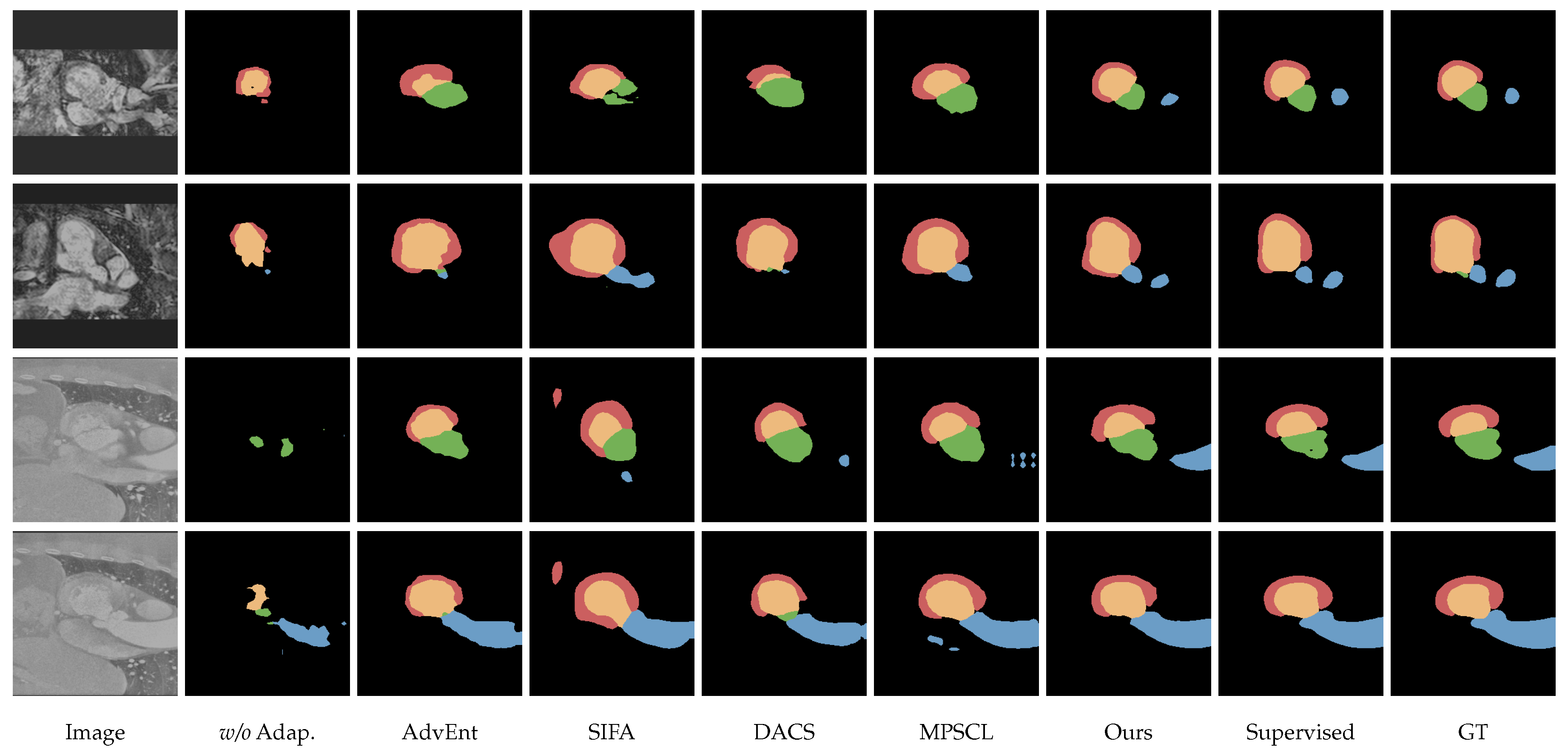
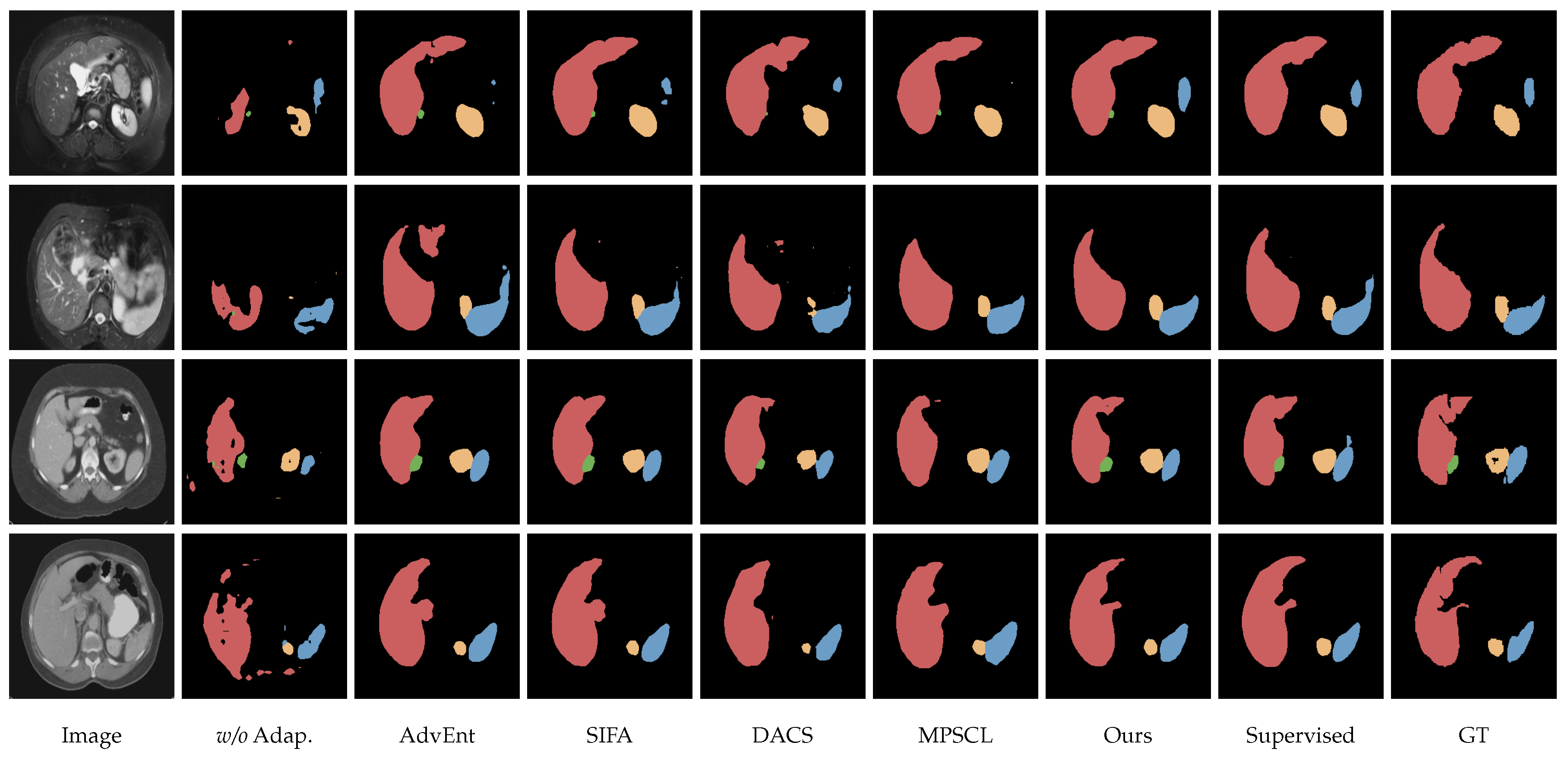
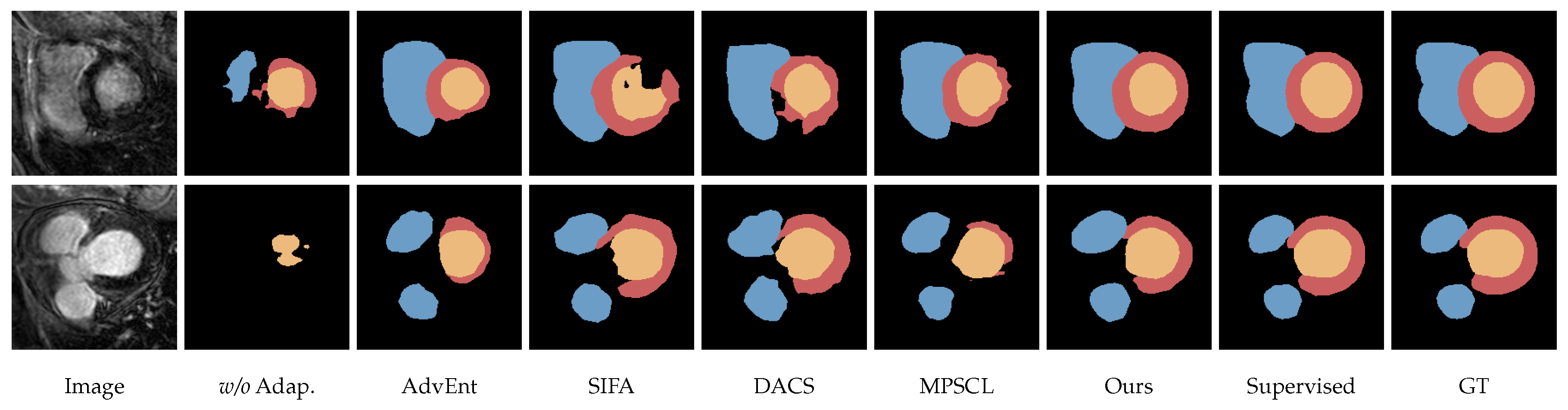
Figure 3, Figure 4 and Figure 5 provide qualitative comparisons on the MM-WHS, Abdominal Multi-Organ, and MS-CMRSeg datasets. The visualized competing methods include the reproduced UDA baselines used in the paired tests. Across the five adaptation tasks, the paired tests showed significant improvements over AdvEnt, SIFA, DACS, and MPSCL in volume-level average Dice value; the maximum observed p value was 0.0270. The qualitative examples show a consistent trend, as the proposed method reduces missing regions, fragmentation, isolated artifacts, and local boundary mismatches relative to the illustrated baselines. These representative cases illustrate the main benchmark trends and should be interpreted together with the failure-case analysis.

4.3. Ablation Studies

To further examine how each design choice contributes to the proposed framework, we conduct a series of diagnostic ablation studies on the representative Cardiac MR→CT adaptation task. We separate the framework into two main methodological branches, then analyze their internal components. The source-side branch, referred to as target-informed fractional texture perturbation (TIFTP), consists of soft histogram-based intensity transfer (SHT) and fractional texture-guided perturbation (FTP). The target-side branch, referred to as boundary-aware pseudo-label perturbation (BAPLP), consists of boundary logit perturbation (BLP), entropy-aware weighting (EW), and fractal boundary-aware weighting (FW). The baseline is a student–teacher cross-domain consistency model trained with source supervision and target pseudo-label consistency, without TIFTP or BAPLP.

The component, operator, mixing, and sensitivity analyses use Cardiac MR→CT as a fixed reference setting. This evaluates individual design choices under a common configuration and avoids confounding from changes in task, dataset, or adaptation direction. Unless otherwise stated, these diagnostic values are obtained from one representative run. Seed-level variability of the complete method is reported in the principal benchmark tables. Throughout

Table 5. Component ablation of the proposed framework on Cardiac MR→CT. SHT and FTP form the source-side TIFTP branch, whereas BLP, EW, and FW form the target-side BAPLP branch. Values are obtained in the fixed diagnostic setting. Bold and underlined values indicate the best and second-best results, respectively.

SHT	FTP	BLP	EW	FW	mDice ↑	mASD ↓	mHD95 ↓	SD@1 ↑	SD@2 ↑	SD@3 ↑	BF1@2 ↑
					84.14	4.47	27.45	42.53	59.71	72.24	60.00
✓					87.23	3.38	18.81	49.84	67.21	78.53	67.45
✓	✓				88.01	3.12	15.22	51.69	69.10	80.11	69.33
		✓			86.23	4.19	24.35	47.31	64.78	76.15	65.04
		✓	✓		86.98	3.04	14.93	49.25	66.60	78.35	66.87
		✓	✓	✓	87.51	2.76	12.42	50.50	67.89	79.42	68.19
✓	✓	✓	✓	✓	89.23	2.07	6.98	54.57	72.06	83.07	72.25

,

Table 6. Comparison of source-side transformation and perturbation strategies on Cardiac MR→CT. The complete TIFTP branch consists of SHT, followed by FTP. “Target-informed” indicates whether target-domain information is used to guide the source modification. Bold and underlined values indicate the best and second-best results, respectively.

Source-Side Strategy	Target-Informed	mDice ↑	mASD ↓	mHD95 ↓	SD@1 ↑	SD@2 ↑	SD@3 ↑	BF1@2 ↑
None		84.14	4.47	27.45	42.53	59.71	72.24	60.00
Random noise		83.93	4.52	27.32	42.03	59.20	71.83	59.50
Adversarial perturbation (FGSM)		85.34	4.27	24.85	45.37	62.62	74.52	62.89
Adversarial perturbation (BIM)		86.02	4.11	23.51	46.98	64.27	75.84	64.53
Adversarial perturbation (PGD)		85.88	3.86	21.19	46.65	63.93	75.78	64.19
SHT only	✓	87.23	3.38	18.81	49.84	67.21	78.53	67.45
SHT + FTP (TIFTP branch)	✓	88.01	3.12	15.22	51.69	69.10	80.11	69.33

,

Table 7. Ablation of boundary-aware pseudo-label perturbation and adaptive weighting on Cardiac MR→CT. BLP, EW, and FW are subcomponents of the target-side BAPLP branch. Bold and underlined values indicate the best and second-best results, respectively.

Pseudo-Label Strategy	BLP	EW	FW	mDice ↑	mASD ↓	mHD95 ↓	SD@1 ↑	SD@2 ↑	SD@3 ↑	BF1@2 ↑
Hard pseudo-label				84.14	4.47	27.45	42.53	59.71	72.24	60.00
Boundary perturbation only	✓			86.23	4.19	24.35	47.31	64.78	76.15	65.04
Entropy-weighted supervision		✓		86.72	3.53	18.70	48.63	65.97	77.51	66.22
Fractal-weighted supervision			✓	86.61	3.32	17.02	48.37	65.70	77.47	65.95
Boundary perturbation + entropy	✓	✓		86.98	3.04	14.93	49.25	66.60	78.35	66.87
Boundary perturbation + entropy and fractal	✓	✓	✓	87.51	2.76	12.42	50.50	67.89	79.42	68.19

,

Table 8. Effect of fractional-order selection in FTP on Cardiac MR→CT. SHT is kept fixed for all settings. Bold and underlined values indicate the best and second-best results, respectively.

Fractional Order Set $\mathcal{V}$	mDice ↑	mASD ↓	mHD95 ↓	SD@1 ↑	SD@2 ↑	SD@3 ↑	BF1@2 ↑
$\left\{1.0\right\}$	87.02	3.83	21.11	49.34	66.70	77.82	66.94
$\left\{0.7\right\}$	86.43	4.08	23.12	47.95	65.27	76.59	65.52
$\left\{1.3\right\}$	86.74	3.58	19.11	48.68	66.02	77.51	66.27
$\{0.7,1.0\}$	87.63	3.99	22.40	50.79	68.18	78.79	68.41
$\{1.0,1.3\}$	87.20	3.47	18.22	49.77	67.14	78.41	67.38
$\{0.7,1.0,1.3\}$	88.01	3.12	15.22	51.69	69.10	80.11	69.33

,

Table 9. Comparison of the multi-order fractional texture descriptor with alternative texture operators on Cardiac MR→CT. SHT is kept fixed for all settings. Bold and underlined values indicate the best and second-best results, respectively.

Texture Operator	mDice ↑	mASD ↓	mHD95 ↓	SD@1 ↑	SD@2 ↑	SD@3 ↑	BF1@2 ↑
None (SHT only)	87.23	3.38	18.81	49.84	67.21	78.53	67.45
Sobel gradient	87.58	3.43	17.90	50.67	68.06	79.11	68.29
Laplacian	86.70	3.98	22.32	48.59	65.92	77.14	66.17
Wavelet detail	87.49	3.36	17.34	50.46	67.84	79.01	68.07
Gabor bank	87.10	3.75	20.47	49.53	66.89	78.02	67.13
Fourier high-pass	86.90	3.84	21.19	49.06	66.41	77.60	66.65
LBP	86.58	4.03	22.72	48.30	65.63	76.89	65.88
Multi-order fractional (ours)	88.01	3.12	15.22	51.69	69.10	80.11	69.33

and

Table 10. Local sensitivity of key hyperparameters on Cardiac MR→CT. Each parameter is evaluated in its corresponding component-specific setting after the default settings are fixed. Bold and underlined values indicate the best and second-best results within each parameter group, respectively.

Parameter	Value	mDice ↑	mASD ↓	mHD95 ↓	SD@1 ↑	SD@2 ↑	SD@3 ↑	BF1@2 ↑
${ϵ}_{\mathrm{frac}}$	0.01	87.45	3.54	18.78	50.36	67.74	78.80	67.98
${ϵ}_{\mathrm{frac}}$	0.02	88.01	3.12	15.22	51.69	69.10	80.11	69.33
${ϵ}_{\mathrm{frac}}$	0.03	87.62	3.41	17.74	50.76	68.15	79.20	68.39
${ϵ}_{\mathrm{frac}}$	0.04	87.18	3.68	19.91	49.72	67.09	78.22	67.33
${\sigma }_w$	0.1	86.46	3.87	21.44	48.02	65.34	76.80	65.59
${\sigma }_w$	0.2	86.72	3.53	18.70	48.63	65.97	77.51	66.22
${\sigma }_w$	0.3	86.37	3.91	21.76	47.81	65.12	76.61	65.38
${\sigma }_w$	0.5	86.03	4.07	23.04	47.00	64.30	75.89	64.56
$\eta$	0.1	85.93	3.56	18.95	46.76	64.05	76.09	64.32
$\eta$	0.2	86.27	3.59	19.19	47.57	64.88	76.67	65.13
$\eta$	0.4	86.61	3.32	17.02	48.37	65.70	77.47	65.95
$\eta$	0.6	86.11	3.47	18.22	47.19	64.49	76.48	64.75

, mDice, surface Dice, and BF1 are reported as percentages, whereas mASD and mHD95 are reported in preprocessed voxel units.

Table 5 shows that the two branches contribute in complementary ways. On the source side, SHT increases mDice from 84.14 to 87.23 and markedly reduces surface errors, indicating that target-related low-order intensity statistics account for an important part of the cross-modality appearance gap. Adding FTP further increases mDice to 88.01 and reduces mHD95 from 18.81 to 15.22, suggesting that fractional texture- and transition-aware perturbation provides additional benefit beyond histogram-level intensity transfer. The target-side branch exhibits a different pattern. BLP mainly improves region overlap, whereas EW and FW more clearly reduce surface-distance errors by limiting the influence of uncertain boundary supervision. When the two branches are combined, the framework achieves the best value for every reported metric in this fixed diagnostic setting, including values of 89.23 for mDice, 2.07 for mASD, and 6.98 for mHD95. These component-level results support the intended division of roles: TIFTP improves source-side appearance robustness, while BAPLP improves reliability-aware target-boundary supervision.

4.3.1. Effect of the Source-Side TIFTP Branch

We next isolate the source-side branch by comparing different ways of modifying the labeled source images. SHT introduces target-related low-order intensity statistics, whereas FTP generates magnitude-normalized perturbations from the source–target fractional texture discrepancy. Although SHT is an intensity transformation rather than a perturbation operation, it is included in the same comparison because it forms the first step of the complete TIFTP branch.

Table 6 compares generic perturbations, adversarial perturbations, intensity transfer, and the complete target-informed source branch. Random noise does not improve the overall metric profile, indicating that arbitrary appearance variation is insufficient for this cross-modality setting. Adversarial perturbations provide moderate gains over the baseline, but they remain weaker than the target-informed strategies. A plausible explanation is that generic or loss-maximizing perturbations mainly reflect local model sensitivity, whereas the modality shift in this task involves structured intensity, texture, and edge-transition changes. Among the tested source-side strategies, SHT is the strongest individual transformation. Adding FTP further improves performance to 88.01 mDice, 3.12 mASD, and 15.22 mHD95. Relative to SHT alone, FTP increases Dice values by 0.78 percentage points and reduces mHD95 by 3.59, supporting the use of target-referenced fractional texture cues for source-side perturbation.

4.3.2. Effect of the Target-Side BAPLP Branch

We then evaluate the target-side branch by comparing different pseudo-label learning strategies. The initial target pseudo-labels are generated by the teacher model. BLP, EW, and FW are introduced independently or progressively to examine their roles in local boundary perturbation and reliability-aware supervision. In the FW-only variant, the pseudo-label boundary and its fractal dimension are still computed for reliability weighting, while logit perturbation is disabled.

Table 7 separates the effects of boundary perturbation and reliability weighting. BLP increases the mDice from 84.14 to 86.23 by training the student with local alternatives around teacher-predicted boundaries, although the improvement in surface-distance metrics is limited when BLP is used alone. EW and FW produce larger reductions in mASD and mHD95, which is consistent with their role in suppressing unreliable pseudo-label supervision rather than generating new appearance variation. Combining BLP with EW improves both overlap and boundary metrics, and adding FW further reduces mHD95 from 14.93 to 12.42. The complete BAPLP branch reaches vales of 87.51 for mDice, 2.76 for mASD, and 68.19 for BF1@2. These results suggest that predictive entropy and fractal boundary complexity provide complementary reliability cues: entropy reflects local probabilistic ambiguity, whereas fractal complexity captures the irregularity of the predicted boundary geometry.

4.3.3. Analysis of Fractal Boundary Complexity

We further analyze how the box-counting fractal dimension contributes to BAPLP. During adaptation, $D_f$ is computed only from the teacher-generated pseudo-label boundary and serves as a label-free descriptor of multi-scale geometric complexity. It is not treated as a calibrated probability of pseudo-label correctness. This distinction is important because a complex boundary can arise from genuine anatomical shape variation as well, as from segmentation fragmentation. Therefore, predictive entropy and fractal complexity describe different aspects of pseudo-label reliability: entropy measures local class uncertainty, whereas FD describes the global irregularity of the predicted boundary. A larger normalized FD expands the region and scale over which boundary sensitivity is probed, while the corresponding fractal weight reduces the loss contribution from that boundary region. Thus, the method explores more local alternatives around complex contours without assigning stronger supervision to those regions.

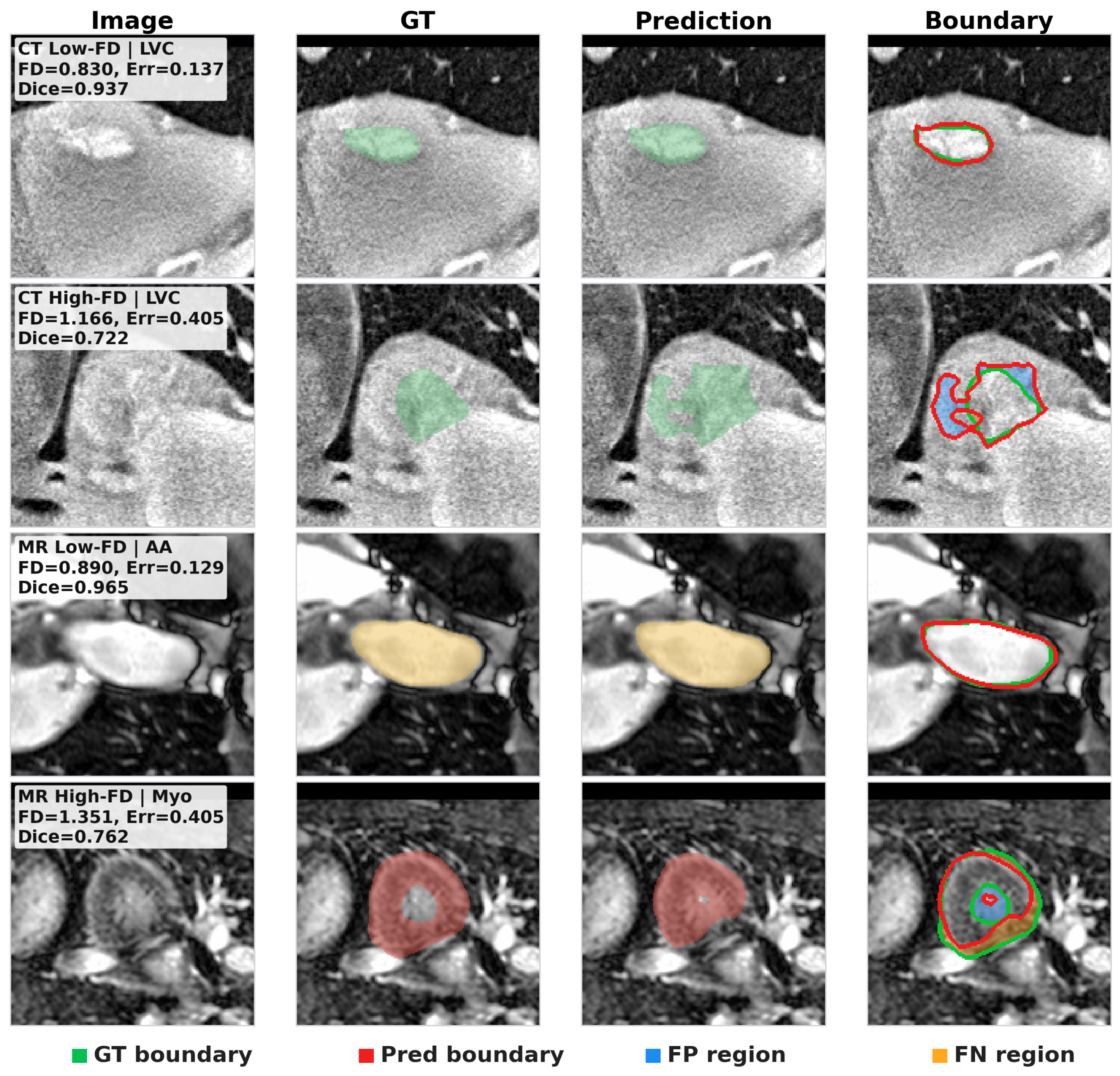
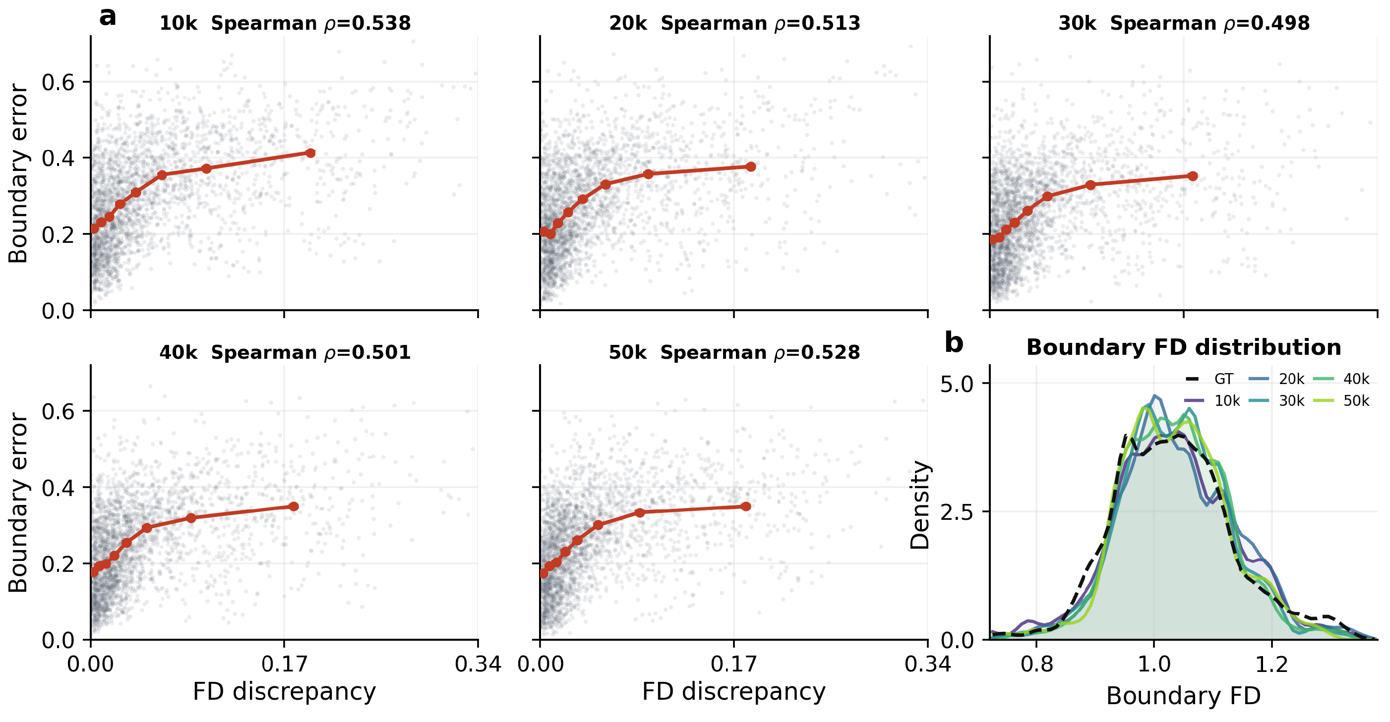
Figure 6 illustrates the type of geometry captured by FD. The examples are selected according to the fractal dimension of the teacher-generated pseudo-label boundary. Low-FD contours are generally smoother, whereas high-FD contours show more local fragmentation. The reference overlays also show why FD should be used as a complementary prior rather than as a direct correctness score: pseudo-label quality depends on the anatomical context and local prediction uncertainty, as well as boundary geometry. To examine the relationship between boundary geometry and pseudo-label quality, we therefore conduct a retrospective reference-based analysis at several checkpoints using the absolute discrepancy between pseudo-label and reference boundary dimensions: $\Delta D_f=\left|D_f\left(B_{\mathrm{PL}}\right)-D_f\left(B_{\mathrm{GT}}\right)\right|.$ Reference annotations are used only for this retrospective analysis. They are not used for adaptation, pseudo-label generation, hyper-parameter selection, or model selection. During training, the FW term depends exclusively on the teacher-generated pseudo-label geometry ($D_f\left(B_0\right)$).

Figure 7 shows a moderate positive association between $\Delta D_f$ and pseudo-label boundary error, with Spearman coefficients ranging from 0.498 to 0.538 between 10,000 and 50,000 iterations. The binned summaries follow the same trend, and the pseudo-label FD distribution becomes closer to the reference distribution as adaptation proceeds. These observations suggest that boundary geometry is related to pseudo-label quality, but they do not establish FD a standalone error estimator. The training-time ablation provides complementary evidence for using FD during training: adding FW to BLP+EW increases the mDice from 86.98% to 87.51%, reduces mASD from 3.04 to 2.76, and reduces mHD95 from 14.93 to 12.42. Taken together, the retrospective analysis and controlled ablation support the use of FD as a secondary geometric prior alongside predictive entropy.

4.3.4. Effect of Fractional-Order Selection in FTP

The fractional-order set ($\mathcal{V}$) controls the type of texture and edge-transition information captured by FTP. In this experiment, SHT is kept fixed, and only the fractional-order set used in FTP is varied. This design isolates the effect of multi-order fractional texture modeling within the source-side branch.

Table 8 shows that the complete-order setoutperforms all single- and two-order variants across the reported overlap and boundary metrics. The single low-order setting ($\left\{0.7\right\}$) is less effective for boundary localization, whereas $\left\{1.3\right\}$ improves the distance metrics relative to the lower orders, suggesting greater sensitivity to sharper local variations. The two-order subsets show different overlap–surface trade-offs. Overall, these results are consistent with the interpretation that the three orders contribute complementary sensitivity to smooth transitions, standard gradients, and sharper texture changes. They provide empirical support for using the compact multi-order configuration in this task.

4.3.5. Effect of Texture-Operator Selection

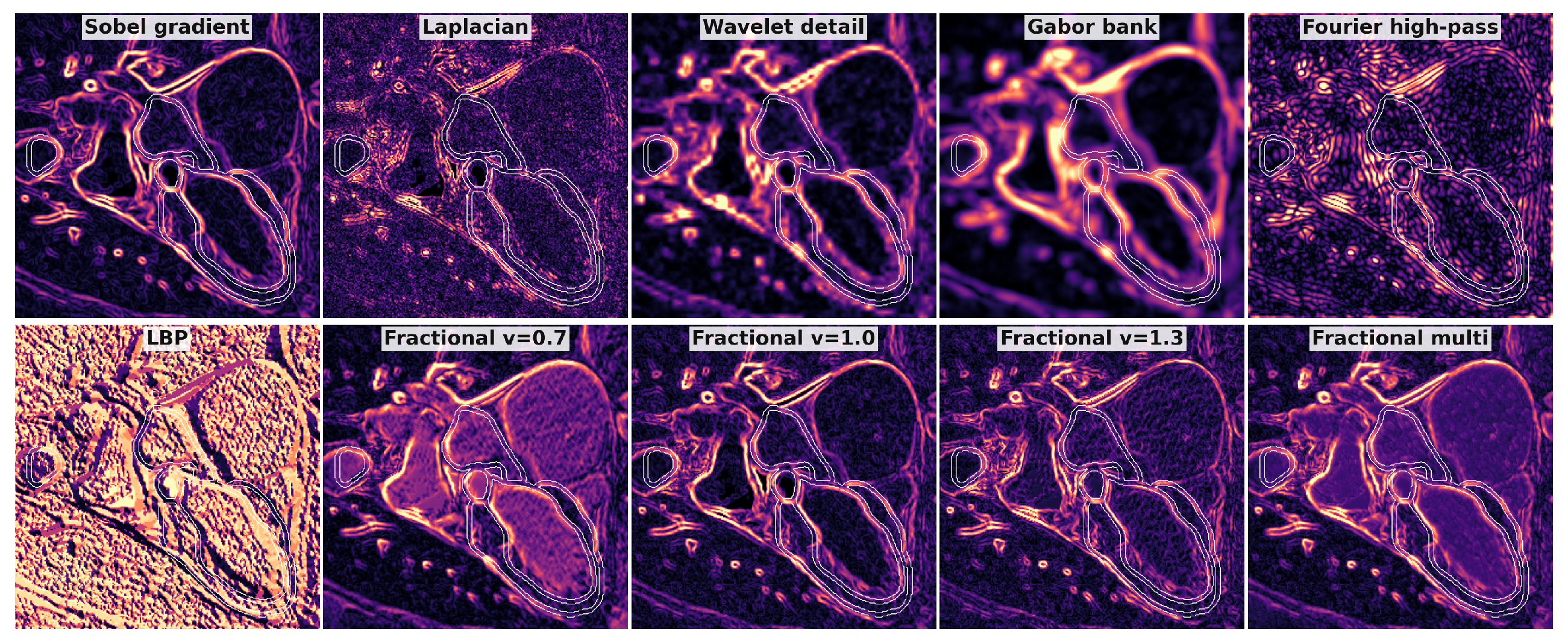
To assess whether the gain is attributable to the fractional response itself or simply to the introduction of a texture operator, we replace the multi-order fractional response with several commonly used texture and boundary operators while keeping the remaining TIFTP pipeline unchanged. Each operator is used to construct a source–target statistic and a magnitude-normalized perturbation direction. Thus, the comparison evaluates operator suitability within the same perturbation-generation procedure rather than treating handcrafted descriptors as standalone segmentation features or claiming a universal ranking among texture descriptors.

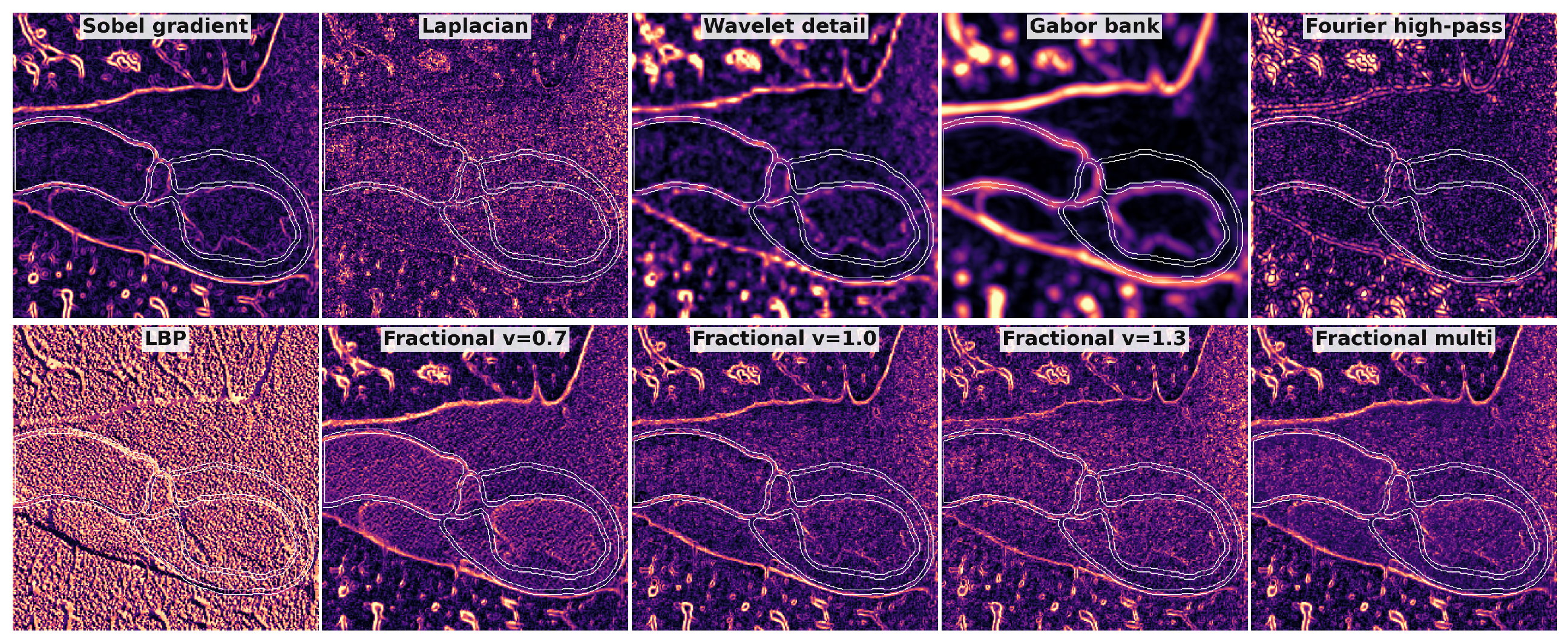
Table 9 shows that the multi-order fractional response achieves the best overall performance among the tested operators under the shared pipeline. Among the alternatives, Sobel provides the strongest overlap-related scores and is closely related to the standard first-order response, whereas wavelet detail provides the strongest distance-related scores. Laplacian, Fourier high-pass, Gabor, and LBP variants emphasize more restricted edge, frequency, orientation, or local-pattern cues and are less balanced in this perturbation setting. Instead, the fractional formulation combines these regimes within a compact, continuously ordered family where $\nu <1$, $\nu =1$, and $\nu >1$ emphasize progressively differentiatedlocal variations. This supports the use of the multi-order fractional response as the perturbation statistic in TIFTP.

The response maps in Figure 8 provide a qualitative view of these differences. Fixed operators tend to isolate particular edge, frequency, orientation, or local-pattern components. In contrast, the combined fractional response retains smoother transition regions while also highlighting first-order edge responses and finer local changes. These patterns help explain why the fractional descriptor is suitable for generating target-referenced perturbations in this pipeline. Importantly, the fractional discrepancy is not used as a direct texture-alignment loss between unpaired source and target slices; it is used only to construct label-preserving source perturbations.

4.3.6. Sensitivity to Perturbation and Weighting Parameters

We examine local sensitivity around the default values of three parameters: the source perturbation magnitude (${ϵ}_{\mathrm{frac}}$), the entropy-weighting bandwidth (${\sigma }_w$), and the fractal down-weighting coefficient ($\eta$). This analysis is performed after the default settings are fixed and is intended as a post hoc stability check rather than target-label-based hyper-parameter tuning. Each parameter is varied only in the component where it is introduced, with the remaining settings held fixed. Specifically, ${ϵ}_{\mathrm{frac}}$ is varied in the source branch with SHT fixed, ${\sigma }_w$ is varied in entropy-weighted supervision, and $\eta$ is varied in fractal-weighted supervision.

Table 10 indicates that moderate perturbation and weighting strengths perform best in this local sweep. For ${ϵ}_{\mathrm{frac}}$, the default value of 0.02 outperforms both weaker and stronger source perturbations. A smaller value may provide insufficient target-relevant texture variation, whereas a larger value may disturb source appearance enough to weaken the label-preserving assumption. For ${\sigma }_w$, the default value of 0.2 provides the best balance between suppressing high-entropy pseudo-labels and retaining useful supervision from moderately uncertain pixels. For $\eta$, the default value of 0.4 results in the best overall metric profile, suggesting that geometrically complex boundary regions should be down-weighted with moderate strength. Overall, the results suggest that the adopted defaults lie in a locally stable region, while overly weak or overly aggressive perturbation or weighting settings can reduce performance.

4.3.7. Evaluation of Cross-Domain Mixing Strategies

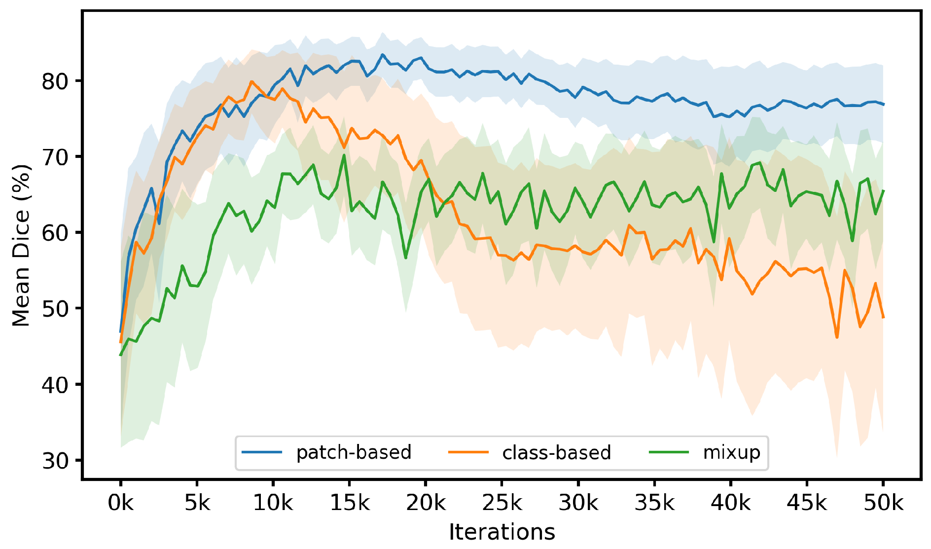
Cross-domain mixing is applied after source labels, target pseudo-labels, and target reliability weights have been constructed. The same binary mask is used for the image, label, and weight maps, preserving the correspondence between each mixed region and its supervision signal. Thus, mixing functions as part of the consistency-learning pathway rather than as an independent augmentation. The default implementation uses random rectangular patch masks in the spirit of CutMix [14]. We compare this strategy with mixup [47] and class-based mixing [48] on Cardiac MR→CT while holding the remaining components fixed. Figure 9 shows that patch-based mixing reaches the highest final Dice value and the smoothest late-stage trajectory in this experiment. Mixup performs worse, plausibly because linear interpolation creates intermediate appearances and soft boundaries that are unrealistic for CT or MR segmentation. Class-based mixing preserves semantic regions, but it depends directly on the current target pseudo-label topology. When early pseudo-labels contain boundary leakage or small-structure errors, these errors can be propagated into the mixed supervision target. Patch masks are less dependent on class topology while preserving local image–label consistency within each region. These observations motivate the use of patch-based mixing as the default strategy, although the comparison is specific to the evaluated task and configuration.

4.3.8. Computational Complexity and Efficiency

Finally, we analyze computational complexity and efficiency on the Cardiac MR→CT task. The proposed perturbation and reliability modules are used only during adaptation, so they increase training-time computation but do not change the deployed segmentation network or its inference-time parameters, MACs, and FLOPs.

Table 11. Computational complexity and efficiency on Cardiac MR→CT using the same hardware and implementation environment. Inference parameters and computation include only components retained at deployment, whereas training-loaded parameters include all networks instantiated during adaptation. The mDice column corresponds to the representative run used for the efficiency measurements. Runtime values are implementation- and hardware-dependent.

	Parameters		Inference Computation		Runtime			Training Memory	Performance
Method	Inference Params (M)	Train-Loaded Params (M)	MACs (G)	FLOPs (G)	Train/Iter (s)	Est. Total @50k (h)	Infer/Image (s)	Peak Alloc./Res. (MiB)	mDice (%) ↑
AdvEnt [42]	42.948	48.587	81.839	163.678	0.3674	5.10	0.0231	4135.4/4350.0	74.44
SIFA [8]	27.528	43.343	29.121	58.241	0.8943	12.42	0.0327	2838.0/3352.0	74.05
DACS [11]	42.948	86.106	81.839	163.678	0.3893	5.41	0.0222	4193.1/4382.0	79.88
MPSCL [18]	42.948	48.587	81.839	163.678	0.5299	7.36	0.0237	4135.4/4350.0	83.02
Ours	42.948	86.106	81.839	163.678	0.6132	8.52	0.0227	4193.1/4382.0	89.23

separates adaptation cost from deployment cost. The proposed method loads the student and EMA teacher and adds fractional perturbation and boundary-reliability computations, resulting in 86.106 M training-loaded parameters and 0.6132 s per iteration. This corresponds to approximately 8.52 h for 50,000 iterations. After adaptation, only the DeepLab-v2 segmentation network is retained, with the same inference-parameter count, MACs, and FLOPs as the same-backbone DACS implementation. Compared with reproduced MPSCL, the method uses about 15.7% more time per training iteration and achieves a 6.21-point higher representative-run mDice. The main trade-off is additional offline adaptation time without added deployment-time complexity; runtime values remain implementation- and hardware-dependent.

4.4. Within-Benchmark Robustness and Failure Analysis

To assess within-benchmark robustness, we examine one representative final model on the Cardiac MR→CT target CT test split, which contains four 3D volumes and 527 foreground-containing slices. Because scanner and institution metadata are unavailable in the released benchmark files, we use slice-level appearance proxies, together with controlled scanner-style perturbations. Clean performance is summarized across the four target volumes with an exploratory volume-bootstrap interval, and the stress tests quantify sensitivity to changes in intensity, contrast, smoothness, bias field, and noise. This analysis complements the three-seed benchmark summary in Table 2; it is not intended as an external scanner- or institution-level validation.

Table 12. Within-benchmark robustness analysis of one representative adapted model on the Cardiac MR→CT target CT test split. Slice-level correlations summarize appearance-proxy associations, and distances are reported in preprocessed voxel units because the stored arrays do not include physical spacing metadata.

Analysis	Metric	Finding
Clean target-volume performance	mDice	mean ± SD: $89.01\pm 1.15$; exploratory 95% volume-bootstrap interval: 88.32–90.17
Boundary error vs. intensity variation	Spearman correlation	Intensity SD: $\rho =0.470$; foreground–background contrast: $\rho =0.480$
Boundary error vs. texture/edge proxies	Spearman correlation	90th-percentile gradient magnitude: $\rho =0.444$; high-frequency residual SD: $\rho =0.323$
Synthetic perturbation stress test	Largest mDice drop	0.61 percentage points under additive noise with $\sigma =0.10$
Other scanner-style perturbations	mDice change	Intensity shift, contrast, gamma, blur, and bias field change mDice by less than 0.22 points
Clean surface robustness	ASD/HD95/BF1@2/SD@3	1.95/6.15/71.77/82.72
Worst perturbation surface robustness	ASD/HD95/BF1@2/SD@3	Additive noise: 2.05/6.44/69.99/81.32

shows moderate positive associations between boundary error and the selected intensity, contrast, gradient, and high-frequency proxies. Because the analysis is slice-based and the test set contains only four independent volumes, these correlations should be interpreted descriptively rather than as patient-level evidence. Under the tested synthetic perturbations, additive noise produces the largest mDice decrease of 0.61 percentage points, while intensity shift, contrast, gamma, blur, and bias-field changes each alter mDice by less than 0.22 points. The corresponding changes in ASD and HD95 are also small in this within-benchmark stress test. These results indicate limited sensitivity to the tested perturbation magnitudes on this benchmark, while validation on independently acquired scanner and institution cohorts remains necessary.

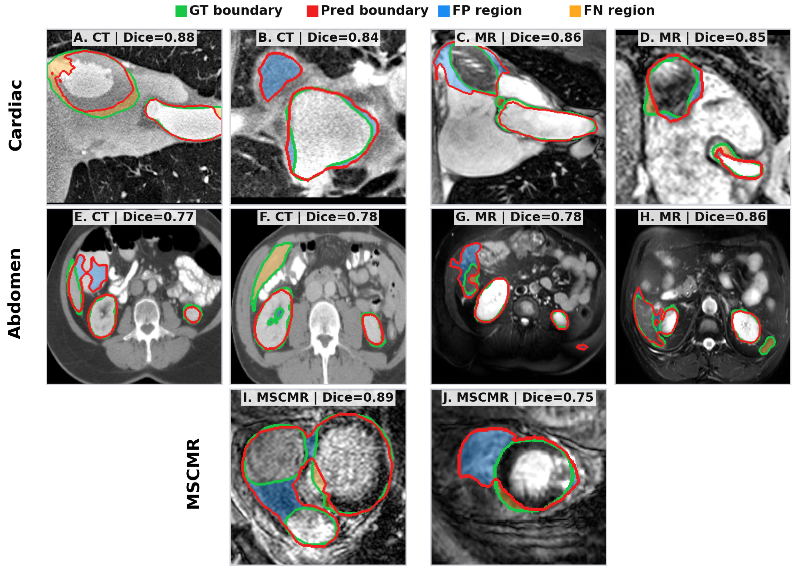
Figure 10 presents representative residual errors across the three benchmarks. In these examples, the coarse anatomical layout is generally retained, but local failures remain around low-contrast boundaries, small structures, and adjacent organs with similar appearance. Cardiac CT/MR cases include local contour shifts, boundary under-segmentation, and small false-positive components around chamber regions. Abdominal cases show adjacent-organ leakage and partial omission of elongated structures, which are difficult to resolve with slice-wise context alone. MS-CMRSeg cases include chamber-like false positives near the myocardium under sequence shift. These examples indicate that the proposed adaptation strategy improves global anatomical consistency, but fine boundary placement, small-structure discrimination, and slice-wise ambiguity remain unresolved failure modes.

5. Discussion

Overall, the results support treating cross-modality UDA as two coupled problems: improving source-side appearance robustness and controlling target-side pseudo-label reliability. TIFTP constructs target-informed source variations while preserving source supervision, and BAPLP probes target-boundary sensitivity while down-weighting unreliable pseudo-label regions. The five-task benchmark results and the boundary-oriented diagnostics on Cardiac MR→CT support this two-pathway design.

The source pathway is formulated as perturbation-based adaptation rather than direct minimization of a source–target feature distance. In medical UDA, unpaired source and target slices may differ not only in modality appearance but also in slice position, anatomical content, and foreground proportion. Therefore, directly forcing their feature statistics to coincide can confound modality-related appearance shift with genuine anatomical variation. By contrast, the proposed fractional discrepancy is used only to derive source-image perturbation directions. This retains standard supervised learning on labeled source data while exposing the student to target-related intensity, texture, and edge-transition variations. The ablation results support this design: SHT accounts for much of the low-order intensity gap, and FTP further improves overlap and boundary metrics. The weaker results with random noise and adversarial perturbations indicate that source variations are more useful when tied to the observed modality discrepancy rather than added as generic noise.

The fractional-order and operator-replacement studies further clarify the role of the fractional formulation. The compact order set $\{0.7,1.0,1.3\}$ combines sensitivity to smoother transitions, first-order edge responses, and sharper local texture changes. Within the shared perturbation-generation pipeline, this multi-order response achieves the most balanced overlap and boundary performance. Sobel and wavelet alternatives remain competitive on some measures, showing that fixed-gradient and multiscale operators also capture useful cues. Thus, the results support the suitability of the multi-order fractional statistic in this framework, without claiming universal superiority.

The target pathway plays a different role. Teacher pseudo-labels provide dense target-domain supervision, but treating them as fixed hard labels can reinforce boundary errors during self-training. Therefore, BAPLP perturbs normalized teacher logits only within predicted boundary bands, allowing the student to learn from local contour alternatives instead of a single unstable boundary. Entropy and fractal weighting then regulate how strongly these perturbed pseudo-labels contribute to optimization. Predictive entropy reflects local class ambiguity, whereas the box-counting fractal dimension provides a complementary description of boundary irregularity and fragmentation. The association between fractal-dimension discrepancy and pseudo-label boundary error, together with the incremental gain from FW in the ablation study, supports the use of the FD as a secondary geometric reliability cue. At the same time, complex anatomy may also produce a high FD, even when the contour is correct. For this reason, the FD is combined with entropy and used as a complementary prior, not as a calibrated estimator of pseudo-label correctness.

The performance patterns across datasets are consistent with the anatomical and modality characteristics of the benchmarks. On MM-WHS, the proposed method achieves the best average Dice and average ASD among the UDA entries for both adaptation directions, indicating strong cardiac cross-modality adaptation. On the Abdominal Multi-Organ benchmark, the method provides the best average overlap for MR→CT and remains within 0.07 percentage points of the highest reported UDA-average Dice score for CT→MR. However, surface-distance performance on the abdominal tasks varies across organs, directions, and comparison protocols, with some recent methods reporting lower ASD values in particular settings. On MS-CMRSeg, the method improves both average overlap and average surface-distance performance under the adopted bSSFP→LGE protocol. The qualitative and failure-case analyses are consistent with these trends: successful cases show more complete regions and cleaner boundaries, while residual errors remain around low-contrast contours, thin or elongated structures, adjacent organs, and sequence-dependent cardiac ambiguities.

From a computational perspective, the method trades additional offline adaptation cost for unchanged deployment complexity. The EMA teacher, fractional-gradient computation, and boundary reliability estimation increase training time. After adaptation, these auxiliary operations are removed, and the deployed model keeps the same parameter count, MACs, and FLOPs as the corresponding DeepLab-v2 segmentation backbone. This profile is suitable for offline adaptation when inference-time model size and latency remain constrained. The reported runtime and memory values remain implementation- and hardware-dependent.

Several limitations define the scope of the current evidence. First, the evaluated public benchmarks are standardized and widely used, but they contain a relatively small number of independent volumes and do not provide sufficient scanner or institution metadata for a true multi-center analysis. The within-benchmark robustness analysis using appearance proxies and scanner-style perturbations provides useful diagnostic evidence, but it cannot replace validation on independently acquired external cohorts. Second, the complete method is reported over three random seeds in the principal benchmark tables, whereas most diagnostic ablations are fixed-setting analyses, and many literature baselines are available only as reported point estimates. Therefore, small cross-method or component-level differences should be interpreted cautiously, and for methods not reproduced in our environment, paired per-volume statistical testing would require aligned predictions or reruns for the compared methods. Third, the framework still depends on teacher-generated pseudo-labels. Boundary perturbation and adaptive weighting reduce the influence of uncertain target regions, but severe early teacher errors, very low target contrast, or anatomically ambiguous structures can still compromise pseudo-label supervision. Fourth, the current implementation follows a 2D slice-wise setting and does not exploit inter-slice context, which may limit performance on thin, elongated, or spatially discontinuous structures. Finally, several module parameters are empirical implementation defaults; although the local sensitivity analysis suggests that the selected values lie in a stable range, more automatic or data-adaptive parameter selection would improve usability. Future work should evaluate the framework on larger multi-center datasets with scanner and institution metadata, perform broader multi-seed and paired per-volume analyses, and investigate 3D or hybrid 2D–3D implementations. Further extensions could combine the perturbation-learning strategy with uncertainty calibration, out-of-distribution target detection, or foundation-model-assisted annotation workflows. Overall, the findings support separating source-appearance robustness from target pseudo-label reliability while optimizing both within a shared adaptation framework.

6. Conclusions

We presented a fractional texture-guided and boundary-aware perturbation-learning framework for unsupervised cross-modality medical image segmentation. The method combines target-informed fractional source perturbations with boundary-localized target-logit perturbation and entropy/fractal reliability weighting. Across five adaptation tasks on the MM-WHS, Abdominal Multi-Organ, and MS-CMRSeg dataset, it achieves leading or near-leading Dice values averaged over three seeds among the protocol-aware UDA comparisons, with competitive surface-distance performance. Ablations, robustness diagnostics, computational evaluation, and failure cases support the complementary roles of the source- and target-side pathways while identifying remaining challenges in fine boundaries, small structures, and slice-wise ambiguity. Because all auxiliary modules are used only during adaptation, the deployment keeps the original segmentation architecture and inference-time parameter count. Future work should validate the framework on larger external multi-center cohorts, extend paired statistical analyses, and explore 3D or hybrid implementations.

References

1. Kilim, O.; Olar, A.; Joo, T.; Palicz, T.; Pollner, P.; Csabai, I. Physical imaging parameter variation drives domain shift. Sci. Rep. 2022, 12, 21302. [Google Scholar] [CrossRef] [PubMed]
2. Guan, H.; Liu, M. Domain adaptation for medical image analysis: A survey. IEEE Trans. Biomed. Eng. 2021, 69, 1173–1185. [Google Scholar]
3. Tomar, D.; Lortkipanidze, M.; Vray, G.; Bozorgtabar, B.; Thiran, J.P. Self-attentive spatial adaptive normalization for cross-modality domain adaptation. IEEE Trans. Med. Imaging 2021, 40, 2926–2938. [Google Scholar] [PubMed]
4. Manakov, I.; Rohm, M.; Kern, C.; Schworm, B.; Kortuem, K.; Tresp, V. Noise as domain shift: Denoising medical images by unpaired image translation. In Proceedings of the Domain Adaptation and Representation Transfer and Medical Image Learning with Less Labels and Imperfect Data; Springer: Berlin/Heidelberg, Germany, 2019; pp. 3–10. [Google Scholar]
5. Gholami, A.; Subramanian, S.; Shenoy, V.; Himthani, N.; Yue, X.; Zhao, S.; Jin, P.; Biros, G.; Keutzer, K. A novel domain adaptation framework for medical image segmentation. In Proceedings of the Brainlesion: Glioma, Multiple Sclerosis, Stroke and Traumatic Brain Injuries; Springer: Berlin/Heidelberg, Germany, 2019; pp. 289–298. [Google Scholar]
6. Bateson, M.; Kervadec, H.; Dolz, J.; Lombaert, H.; Ayed, I.B. Constrained domain adaptation for segmentation. In Proceedings of the Medical Image Computing and Computer-Assisted Intervention—MICCAI 2019; Springer: Berlin/Heidelberg, Germany, 2019; pp. 326–334. [Google Scholar]
7. Dou, Q.; Ouyang, C.; Chen, C.; Chen, H.; Glocker, B.; Zhuang, X.; Heng, P.A. PnP-AdaNet: Plug-and-play adversarial domain adaptation network at unpaired cross-modality cardiac segmentation. IEEE Access 2019, 7, 99065–99076. [Google Scholar]
8. Chen, C.; Dou, Q.; Chen, H.; Qin, J.; Heng, P.A. Unsupervised bidirectional cross-modality adaptation via deeply synergistic image and feature alignment for medical image segmentation. IEEE Trans. Med. Imaging 2020, 39, 2494–2505. [Google Scholar] [CrossRef] [PubMed]
9. Xie, Q.; Li, Y.; He, N.; Ning, M.; Ma, K.; Wang, G.; Lian, Y.; Zheng, Y. Unsupervised domain adaptation for medical image segmentation by disentanglement learning and self-training. IEEE Trans. Med. Imaging 2022, 43, 4–14. [Google Scholar]
10. Han, X.; Qi, L.; Yu, Q.; Zhou, Z.; Zheng, Y.; Shi, Y.; Gao, Y. Deep symmetric adaptation network for cross-modality medical image segmentation. IEEE Trans. Med. Imaging 2022, 41, 121–132. [Google Scholar] [PubMed]
11. Tranheden, W.; Olsson, V.; Pinto, J.; Svensson, L. DACS: Domain adaptation via cross-domain mixed sampling. In Proceedings of the IEEE/CVF Winter Conference on Applications of Computer Vision; IEEE: New York, NY, USA, 2021; pp. 1379–1389. [Google Scholar]
12. Zhang, P.; Zhang, B.; Zhang, T.; Chen, D.; Wang, Y.; Wen, F. Prototypical pseudo label denoising and target structure learning for domain adaptive semantic segmentation. In Proceedings of the IEEE/CVF Conference on Computer Vision and Pattern Recognition; IEEE: New York, NY, USA, 2021; pp. 12414–12424. [Google Scholar]
13. Xie, B.; Li, S.; Li, M.; Liu, C.H.; Huang, G.; Wang, G. SePiCo: Semantic-guided pixel contrast for domain adaptive semantic segmentation. IEEE Trans. Pattern Anal. Mach. Intell. 2023, 45, 9004–9021. [Google Scholar] [PubMed]
14. Yun, S.; Han, D.; Oh, S.J.; Chun, S.; Choe, J.; Yoo, Y. CutMix: Regularization strategy to train strong classifiers with localizable features. In Proceedings of the IEEE/CVF International Conference on Computer Vision; IEEE: New York, NY, USA, 2019; pp. 6023–6032. [Google Scholar]
15. Hu, T.; Sun, S.; Zhao, J.; Shi, D. Enhancing unsupervised domain adaptation via semantic similarity constraint for medical image segmentation. In Proceedings of the Thirty-First International Joint Conference on Artificial Intelligence. International Joint Conferences on Artificial Intelligence Organization; IJCAI Organization: Montpellier, France, 2022; pp. 3071–3077. [Google Scholar] [CrossRef] [PubMed]
16. Feng, W.; Wang, L.; Ju, L.; Zhao, X.; Wang, X.; Shi, X.; Ge, Z. Unsupervised domain adaptive fundus image segmentation with category-level regularization. In Proceedings of the International Conference on Medical Image Computing and Computer-Assisted Intervention; Springer: Berlin/Heidelberg, Germany, 2022; pp. 497–506. [Google Scholar]
17. Feng, W.; Ju, L.; Wang, L.; Song, K.; Zhao, X.; Ge, Z. Unsupervised domain adaptation for medical image segmentation by selective entropy constraints and adaptive semantic alignment. Proc. AAAI Conf. Artif. Intell. 2023, 37, 623–631. [Google Scholar] [CrossRef]
18. Liu, Z.; Zhu, Z.; Zheng, S.; Liu, Y.; Zhou, J.; Zhao, Y. Margin preserving self-paced contrastive learning towards domain adaptation for medical image segmentation. IEEE J. Biomed. Health Inform. 2022, 26, 638–647. [Google Scholar] [CrossRef] [PubMed]
19. Yu, Q.; Xi, N.; Yuan, J.; Zhou, Z.; Dang, K.; Ding, X. Source-free domain adaptation for medical image segmentation via prototype-anchored feature alignment and contrastive learning. In Proceedings of the International Conference on Medical Image Computing and Computer-Assisted Intervention; Springer: Berlin/Heidelberg, Germany, 2023; pp. 3–12. [Google Scholar]
20. Dong, S.; Pan, Z.; Fu, Y.; Xu, D.; Shi, K.; Yang, Q.; Shi, Y.; Zhuo, C. Partial unbalanced feature transport for cross-modality cardiac image segmentation. IEEE Trans. Med. Imaging 2023, 42, 1758–1773. [Google Scholar] [CrossRef] [PubMed]
21. Liu, S.; Yin, S.; Qu, L.; Wang, M.; Song, Z. A structure-aware framework of unsupervised cross-modality domain adaptation via frequency and spatial knowledge distillation. IEEE Trans. Med. Imaging 2023, 42, 3919–3931. [Google Scholar] [PubMed]
22. Ji, W.; Chung, A.C.S. Unsupervised Domain Adaptation for Medical Image Segmentation Using Transformer with Meta Attention. IEEE Trans. Med. Imaging 2024, 43, 820–831. [Google Scholar] [CrossRef] [PubMed]
23. En, Q.; Guo, Y. Unsupervised Domain Adaptation for Medical Image Segmentation with Dynamic Prototype-based Contrastive Learning. PMLR 2024, 248, 312–325. [Google Scholar]
24. Ji, W.; Chung, A.C.S. Diffusion-Based Domain Adaptation for Medical Image Segmentation Using Stochastic Step Alignment. In Proceedings of the Medical Image Computing and Computer Assisted Intervention—MICCAI 2024; Lecture Notes in Computer Science; Springer Nature: Cham, Switzerland, 2024; Volume 15008, pp. 188–198. [Google Scholar] [CrossRef]
25. Zhang, X.; Wu, Y.; Angelini, E.; Li, A.; Guo, J.; Rasmussen, J.M.; O’Connor, T.G.; Wadhwa, P.D.; Jackowski, A.P.; Li, H.; et al. MAPSeg: Unified Unsupervised Domain Adaptation for Heterogeneous Medical Image Segmentation Based on 3D Masked Autoencoding and Pseudo-Labeling. In Proceedings of the IEEE/CVF Conference on Computer Vision and Pattern Recognition; IEEE: New York, NY, USA, 2024; pp. 5851–5862. [Google Scholar]
26. Lyu, P.; Yeung, P.H.; Yu, X.; Xia, J.; Chi, J.; Wu, C.; Rajapakse, J.C. Bridging the Inter-Domain Gap through Low-Level Features for Cross-Modal Medical Image Segmentation. arXiv 2025, arXiv:2505.11909. [Google Scholar]
27. Maurya, L.; Liu, H.; Zwiggelaar, R. TCSA-UDA: Text-Driven Cross-Semantic Alignment for Unsupervised Domain Adaptation in Medical Image Segmentation. arXiv 2025, arXiv:2511.05782. [Google Scholar]
28. Ma, A.; Zhu, Q.; Li, J.; Nielsen, M.; Chen, X. Source-Free Domain Adaptation for Cross-Modality Cardiac Image Segmentation with Contrastive Class Relationship Consistency. In Proceedings of the Medical Image Computing and Computer Assisted Intervention—MICCAI 2025; Lecture Notes in Computer Science; Springer Nature: Cham, Switzerland, 2026; Volume 15964, pp. 574–583. [Google Scholar] [CrossRef]
29. Yang, J.; Yu, X.; Qiu, P.; Marcus, D.; Sotiras, A. Active Source-Free Cross-Domain and Cross-Modality Adaptation for Volumetric Medical Image Segmentation by Image Sensitivity and Organ Heterogeneity Sampling. In Proceedings of the Medical Image Computing and Computer Assisted Intervention—MICCAI 2025; Lecture Notes in Computer Science; Springer Nature: Cham, Switzerland, 2026; Volume 15965, pp. 3–12. [Google Scholar] [CrossRef]
30. Kirillov, A.; Mintun, E.; Ravi, N.; Mao, H.; Rolland, C.; Gustafson, L.; Xiao, T.; Whitehead, S.; Berg, A.C.; Lo, W.Y.; et al. Segment Anything. In Proceedings of the IEEE/CVF International Conference on Computer Vision; IEEE: New York, NY, USA, 2023; pp. 4015–4026. [Google Scholar]
31. Radford, A.; Kim, J.W.; Hallacy, C.; Ramesh, A.; Goh, G.; Agarwal, S.; Sastry, G.; Askell, A.; Mishkin, P.; Clark, J.; et al. Learning Transferable Visual Models From Natural Language Supervision. PMLR 2021, 139, 8748–8763. [Google Scholar]
32. Podlubny, I. Fractional Differential Equations; Academic Press: Cambridge, MA, USA, 1999. [Google Scholar]
33. Sparavigna, A.C. Fractional differentiation based image processing. arXiv 2009, arXiv:0910.2381. [Google Scholar]
34. Mandelbrot, B.B. The Fractal Geometry of Nature; W. H. Freeman: San Francisco, CA, USA, 1983. [Google Scholar]
35. Falconer, K. Fractal Geometry: Mathematical Foundations and Applications, 2nd ed.; John Wiley & Sons: Hoboken, NJ, USA, 2003. [Google Scholar]
36. Li, J.; Du, Q.; Sun, C. An improved box-counting method for image fractal dimension estimation. Pattern Recognit. 2009, 42, 2460–2469. [Google Scholar] [CrossRef]
37. Zhuang, X.; Li, L.; Payer, C.; Stern, D.; Urschler, M.; Heinrich, M.P.; Oster, J.; Wang, C.; Smedby, O.; Bian, C.; et al. Evaluation of algorithms for multi-modality whole heart segmentation: An open-access grand challenge. Med. Image Anal. 2019, 58, 101537. [Google Scholar] [PubMed]
38. Landman, B.; Xu, Z.; Igelsias, J.; Styner, M.; Langerak, T.; Klein, A. MICCAI multi-atlas labeling beyond the cranial vault–workshop and challenge. In Proceedings of the MICCAI Multi-Atlas Labeling Beyond Cranial Vault Workshop and Challenge; Synapse: Singapore, 2015; Volume 5, p. 12. [Google Scholar]
39. Kavur, A.E.; Gezer, N.S.; Baris, M.; Aslan, S.; Conze, P.H.; Groza, V.; Pham, D.D.; Chatterjee, S.; Ernst, P.; Ozkan, S.; et al. CHAOS challenge—Combined (CT-MR) healthy abdominal organ segmentation. Med. Image Anal. 2021, 69, 101950. [Google Scholar] [CrossRef] [PubMed]
40. Zhuang, X. Multivariate mixture model for cardiac segmentation from multi-sequence MRI. In Proceedings of the International Conference on Medical Image Computing and Computer-Assisted Intervention; Springer: Berlin/Heidelberg, Germany, 2016; pp. 581–588. [Google Scholar]
41. Wu, F.; Zhuang, X. Unsupervised domain adaptation with variational approximation for cardiac segmentation. IEEE Trans. Med. Imaging 2021, 40, 3555–3567. [Google Scholar] [CrossRef]
42. Vu, T.H.; Jain, H.; Bucher, M.; Cord, M.; Perez, P. ADVENT: Adversarial entropy minimization for domain adaptation in semantic segmentation. In Proceedings of the IEEE/CVF Conference on Computer Vision and Pattern Recognition; IEEE: New York, NY, USA, 2019; pp. 2517–2526. [Google Scholar]
43. Wu, F.; Zhuang, X. CF distance: A new domain discrepancy metric and application to explicit domain adaptation for cross-modality cardiac image segmentation. IEEE Trans. Med. Imaging 2020, 39, 4274–4285. [Google Scholar] [CrossRef] [PubMed]
44. Pei, C.; Wu, F.; Huang, L.; Zhuang, X. Disentangle domain features for cross-modality cardiac image segmentation. Med. Image Anal. 2021, 71, 102078. [Google Scholar] [CrossRef] [PubMed]
45. Wang, R.; Zheng, G. CyCMIS: Cycle-consistent cross-domain medical image segmentation via diverse image augmentation. Med. Image Anal. 2022, 76, 102328. [Google Scholar] [PubMed]
46. Liu, S.; Yin, S.; Qu, L.; Wang, M. Reducing domain gap in frequency and spatial domain for cross-modality domain adaptation on medical image segmentation. Proc. AAAI Conf. Artif. Intell. 2023, 37, 1719–1727. [Google Scholar] [CrossRef]
47. Zhang, H.; Cisse, M.; Dauphin, Y.N.; Lopez-Paz, D. mixup: Beyond empirical risk minimization. arXiv 2017, arXiv:1710.09412. [Google Scholar]
48. Olsson, V.; Tranheden, W.; Pinto, J.; Svensson, L. ClassMix: Segmentation-based data augmentation for semi-supervised learning. In Proceedings of the IEEE/CVF Winter Conference on Applications of Computer Vision; IEEE: New York, NY, USA, 2021; pp. 1369–1378. [Google Scholar]
Figure 1. Motivation for boundary-aware perturbation learning. Panels (a,b) show representative prediction–reference mismatches, with white regions marking disagreement; in these examples, the largest errors occur near anatomical boundaries. Panel (c) illustrates how a small logit perturbation can change the class assigned to a high-entropy boundary pixel, motivating uncertainty-aware treatment of boundary pseudo-labels.
Fractalfract 10 00456 g001
Figure 2. Overview of the proposed student–teacher framework. The source pathway combines soft histogram transfer with target-referenced multi-order fractional perturbation to create appearance variants of labeled source images. The target pathway perturbs teacher logits within predicted boundary bands and weights pseudo-label supervision using predictive entropy and box-counting boundary complexity. The two pathways are optimized jointly through supervised source learning and weighted cross-domain consistency.
Fractalfract 10 00456 g002
Figure 3. Visual comparison of segmentation results on the MM-WHS dataset. From left to right, columns show the input image; segmentation results obtained w/o adaptation; segmentation results obtained using AdvEnt, SIFA, DACS, MPSCL, the proposed method, and supervised training; and the ground truth (GT). The segmented cardiac structures include the ascending aorta (AA, blue), left-atrium blood cavity (LAC, green), left-ventricle blood cavity (LVC, yellow), and left-ventricular myocardium (MYO, red). In the displayed cases, the proposed method reduces large missing regions and shows closer agreement with the reference contours than the illustrated UDA outputs.
Fractalfract 10 00456 g003
Figure 4. Visual comparison of segmentation results on the Abdominal Multi-Organ dataset. From left to right, columns show the input image; segmentation results obtained w/o adaptation; segmentation results obtained using AdvEnt, SIFA, DACS, MPSCL, the proposed method, and supervised training; and the ground truth (GT). The segmented abdominal structures include the liver (red), right kidney (green), left kidney (yellow), and spleen (blue). In the displayed cases, the proposed method shows fewer fragmented regions and more continuous organ contours than the illustrated UDA outputs.
Fractalfract 10 00456 g004
Figure 5. Visual comparison of segmentation results on the MS-CMRSeg dataset. From left to right, columns show the input image; segmentation results obtained w/o adaptation; segmentation results obtained with AdvEnt, SIFA, DACS, MPSCL, the proposed method, and supervised training; and the ground truth (GT). The segmented cardiac structures include the left-ventricular cavity (LVC, yellow), right-ventricular cavity (RVC, blue), and myocardium (MYO, red). In the displayed cases, the proposed method shows fewer isolated artifacts and closer agreement with the reference structures than the illustrated UDA outputs.
Fractalfract 10 00456 g005
Figure 6. Representative CT and MR examples with low and high pseudo-label boundary fractal complexity. Green and red curves indicate reference and predicted boundaries, respectively; reference contours are shown only for visualization. Low- and high-FD examples are selected according to pseudo-label FD. Low-FD cases usually show smoother contours, whereas high-FD cases often contain more fragmented local geometry.
Fractalfract 10 00456 g006
Figure 7. Retrospective analysis of fractal-dimension discrepancy and pseudo-label boundary error. (a) The reference-based discrepancy ( Δ D f ) shows a moderate positive association with boundary error across checkpoints. (b) Density estimates summarize the pseudo-label and reference FD distributions during adaptation. Reference boundaries are used only for this retrospective analysis; the training-time FW term uses pseudo-label geometry alone.
Fractalfract 10 00456 g007
Figure 8. Visual comparison of representative texture-operator responses on CT and MR images. Fixed operators emphasize specific edge, frequency, orientation, or local-pattern responses, whereas the multi-order fractional response provides complementary sensitivity to smooth transitions, first-order edge responses, and fine texture changes.
Fractalfract 10 00456 g008aFractalfract 10 00456 g008b
Figure 9. Dice curves for three cross-domain mixing strategies on Cardiac MR→CT with the remaining components fixed. Patch-based mixing achieves the smoothest late-stage trajectory and the highest final Dice value in the displayed experiment.
Fractalfract 10 00456 g009
Figure 10. Representative failure cases across cardiac, abdominal, and multi-sequence cardiac MR adaptation tasks. The first row shows cardiac CT/MR cases, the second row shows abdominal CT/MR cases, and the final row shows MS-CMRSeg cases. Green and red curves indicate reference and predicted boundaries, while blue and orange regions denote false-positive and false-negative areas.
Fractalfract 10 00456 g010