Identification of Complex Nonlinear Fractional-Order System Based on Fuzzy Multi-Model

Abstract

Fractional-order dynamic systems, due to their long memory and nonlocality, have significant advantages in describing the dynamic behavior of complex engineering systems. However, existing identification methods often struggle to balance modeling accuracy and model structural complexity under conditions of strong nonlinearity, strong coupling, and multiple operating conditions. To address the challenge of modeling complex fractional-order systems with strong nonlinearity, strong coupling, and multiple operating conditions, this paper proposes a fuzzy multi-model modeling and identification method based on the decomposition-synthesis approach. First, a fractional-order fuzzy multi-model structure is constructed to characterize the dynamic characteristics of such complex systems. Second, an improved SKFCM hybrid clustering algorithm is proposed, combining K-means clustering and satisfactory fuzzy C-means clustering. This optimizes the cluster center selection strategy and overcomes the shortcomings of traditional satisfactory FCM algorithms, such as random initial membership and unreasonable cluster center selection, thus achieving a reasonable determination of the number of local models. Finally, the least-squares and Levenberg–Marquardt algorithms are integrated to interactively identify local model parameters, system fractional-order, and fuzzy scheduling function parameters, solving key difficulties such as unknown fractional-order s in antecedent variables, numerous parameter couplings, and difficulty in determining the antecedent space. Through academic examples and simulations of a robotic arm system, the proposed method effectively achieves high-precision modeling of complex fractional-order systems, demonstrating strong feasibility and superiority.

1. Introduction

Modeling and parameter identification of fractional-order dynamic systems has become a research hotspot in the field of engineering control in recent years. Compared with integer-order models, fractional-order calculus has unique long-memory and nonlocality characteristics, enabling it to more accurately describe the intrinsic dynamic behavior of complex systems [1,2]. This advantage has led to the widespread application of fractional-order methods in various engineering fields such as robotic arms [3,4], proton exchange membrane fuel cells [5,6], lithium-ion battery state estimation [7,8], and soft actuators [9], demonstrating capabilities that surpass integer-order modeling.

Fractional-order system identification methods are mainly divided into two categories: frequency domain identification and time domain identification. In the frequency domain, researchers have solved the identification problem of experimental systems of unknown order by constructing nonlinear least-squares problems [10] or using extended sparse regression [11]. The research on time domain identification is more abundant. Duhé et al. established a complete recursive identification framework for continuous-time fractional-order models, covering both known and unknown order cases [12]. For nonlinear systems, identification methods based on block structure models have received widespread attention, such as the parameter decoupling and joint estimation algorithm for the Hammerstein–Wiener model [13,14]. In addition, the least-squares method based on the modulation function [15] and the time domain identification algorithm [16] have verified the superiority of fractional-order models in noise suppression and two-mass system modeling, respectively.

To address the problem that traditional identification methods have a high dependence on prior information, intelligent optimization algorithms have been introduced in large numbers. Particle swarm optimization and its improved algorithms (such as Lévy flight, differential evolution, etc.) have been successfully applied to parameter identification of fractional-order chaotic systems [17], epidemic propagation models [18], and Wiener–Hammerstein systems [19]. Hybrid optimization strategies (such as the combination of particle swarm optimization and genetic algorithms) have further improved the online identification capability of time-varying parameters [20]. These studies transform the identification problem into an optimization problem, reducing the prior requirements for the system model structure.

In practical fractional-order system modeling, the unknown differential order and the need for synchronous identification with system parameters are common technical challenges. To address this problem, researchers have developed various synchronous identification strategies, including a time delay and order synchronization algorithm based on the modified optimal perturbation method [21]; a method using the Legendre wavelet operation matrix to jointly estimate non-homogeneous order, time delay, and coefficients [22]; and a variable-period integral operation matrix technique for measurement noise environments [23]. These methods achieve efficient synchronous identification of order and parameters by constructing special operation matrices or numerical formats.

In the field of nonlinear system identification, fuzzy modeling methods have unique advantages due to their ability to handle uncertainty. Fractional-order learning algorithms based on the Takagi–Sugeno (TS) fuzzy model [24] and fractional-order gradient descent neural fuzzy models [25] have been proven to effectively linearize nonlinear systems. Meanwhile, a series of advances have also been made in observer design and fault estimation methods for TS fuzzy fractional-order systems [26]. However, the aforementioned studies largely assume a known model structure. For real-world systems with unknown model parameters and uncertain structures, data-driven fractional-order fuzzy multi-model identification still faces challenges, primarily in the following aspects: computational difficulties arise from the antecedent variables being fractional-order variables of unknown order; multi-parameter coupling increases algorithm complexity; the number of local models is difficult to determine; and the antecedent space partitioning lacks a scientific basis.

To address these issues, this paper proposes a fractional-order fuzzy multi-model modeling and identification method based on the decomposition-synthesis principle. First, multiple local models are used to describe the global characteristics of complex nonlinear fractional-order systems. Second, K-means clustering is introduced into the satisfactory fuzzy C-means clustering algorithm, constructing an SKFCM hybrid clustering algorithm to accurately determine the number of local models. Finally, the antecedent variables are selected as fractional-order variables of unknown order, and the Levenberg–Marquardt algorithm and least-squares method are combined to achieve interactive identification of local model parameters and fractional-order values.

This paper is structured as follows. Basic concepts of fractional calculus are introduced in Section 1. Section 2 presents a step-by-step account of how the fractional fuzzy multi-model is established. Section 3 proposes the SKFCM clustering algorithm and interactive identification method. Section 4 verifies the effectiveness of the method through examples of academic fractional calculus systems and robotic arm systems; the control application based on the established model will be the focus of the next research step.

2. Model Establishment

2.1. Fractional Calculation

The computation and application of fractional-order systems have attracted considerable research attention due to their widespread use in identification, control, filtering, and fault diagnosis. Various definitions of fractional calculus operators exist in the literature. For discrete-time cases, the most common ones are the Grünwald–Letnikov (GL) [27], Riemann–Liouville (RL) [28], and Caputo [29] definitions. This paper adopts the GL definition, which is given by:

$${\Delta }^{\alpha }x(kh)={\displaystyle \frac{1}{h^{\alpha }}}{\displaystyle \sum _{i=0}^k{(-1)}^i}\left(\begin{array}{l}\alpha \hfill \\ i\hfill \end{array}\right)x((k-i)h)$$

(1)

where ${\Delta }^{\alpha }$ represents the fractional-order difference operator with order $\alpha$, the initial value of which is 0; $x(kh)$ denotes a function of $t=kh$; and $h$ is the system sampling time, $\left(\begin{array}{l}\alpha \hfill \\ i\hfill \end{array}\right)$ is defined by the following binomial equation:

$$\left(\begin{array}{l}\alpha \hfill \\ i\hfill \end{array}\right)=\left\{\begin{array}{ll}1\hfill & \mathrm{for} i=0\hfill \\ {\displaystyle \frac{\alpha (\alpha -1)\cdots (\alpha -i+1)}{i!}}\hfill & \mathrm{for} i>0\hfill \end{array}\right.$$

(2)

The following recurrence relationship is defined as:

$$\left\{\begin{array}{l}\beta (0)=1\hfill \\ \beta (i)=\beta (i-1){\displaystyle \frac{(i-\alpha -1)}{i}} \mathrm{for} i=1,\dots ,k\hfill \end{array}\right.$$

(3)

where $\beta (i)={(-1)}^i\left(\begin{array}{c}\alpha \\ i\end{array}\right)$. By combining Equations (2) and (3), Equation (1) can be written as:

$${\Delta }^{\alpha }x(kh)={\displaystyle \frac{1}{h^{\alpha }}}{\displaystyle \sum _{i=0}^k\beta (i)}x((k-i)h)$$

(4)

Assuming that system sampling time $h=1$, Equation (4) can be written as Equation (5):

$${\Delta }^{\alpha }x(k)={\displaystyle \sum _{i=0}^k\beta }(i)x(k-i)$$

(5)

2.2. Description of Local Model

Fractional-order systems can be represented by various types of models, including differential equations, transfer functions, state–space representations [30,31,32], as well as discrete or continuous forms. In this paper, the following discrete transfer function model is adopted to describe fractional-order systems:

$$y(k)={\displaystyle \frac{B(z)}{A(z)}}u(k)$$

(6)

where $u(k)$ and $y(k)$ are the input and output of the system, and $y(k)=y_0(k)+v(k)$ and $B(z)$ are the denominator polynomial and the numerator polynomial, respectively,

$$A(z)=1+a_1{z}^{-{\alpha }_1}+a_2{z}^{-{\alpha }_2}+\cdots +a_{n_a}{z}^{-{\alpha }_{n_a}} B(z)=b_1{z}^{-{\gamma }_1}+b_2{z}^{-{\gamma }_2}+\cdots +b_{n_b}{z}^{-{\gamma }_{n_b}}$$

where ${\alpha }_i,{\gamma }_i\in R^{+}$ is the fractional order, and $z^{-1}$ is the backshift operator, $z^{-1}y(k)=y(k-1)$. The regression equation of Equation (6) can be expressed as follows:

$$y(k)+{\displaystyle {\displaystyle \sum _{i=1}^{n_a}}{a}_i}{z}^{-{\alpha }_i}y(k)={\displaystyle {\displaystyle \sum _{i=1}^{n_b}}{b}_i}{z}^{-{\gamma }_i}u(k)$$

(7)

If the fractional orders take entirely different values, then the fractional-order models in Equations (6) and (7) usually become systems of non-identical (or disproportionate) order; otherwise, each fractional order is an integer multiple of the base order ($\alpha$ is order factor) ${\alpha }_i=i-\alpha ,{\gamma }_i=j-\alpha$$(i=1,2\dots ,n_a;j=1,2\dots ,n_b)$. Such a model is defined as a homogeneous (proportionate) order system. In this work, a proportional fractional-order system is considered. Then, the regression equation of Equation (7) can be written as:

$$y(k)+{\displaystyle {\displaystyle \sum _{i=1}^{n_a}}{a}_i}{z}^{-i+\alpha }y(k)={\displaystyle {\displaystyle \sum _{i=1}^{n_b}}{b}_i}{z}^{-i+\alpha }u(k)$$

(8)

Using the discrete fractional-order operator $\Delta$ and by combining it with the backshift operator, the model is expressed as follows:

$$y(k)=-{\displaystyle {\displaystyle \sum _{i=1}^{n_a}}{a}_i}{\Delta }^{\alpha }y(k-i)+{\displaystyle {\displaystyle \sum _{i=1}^{n_b}}{b}_i}{\Delta }^{\alpha }u(k-i)$$

(9)

2.3. Establishment of Fractional-Order Fuzzy Multi-Model

The idea behind the fractional-order fuzzy multi-model strategy is the decomposition–synthesis principle. First, the whole system is divided into several fractional-order subsystems according to a certain decomposition principle, and the local model of each subsystem is selected. Afterward, each local model parameter and each parameter of the dispatch function are identified. Finally, according to a certain scheduling mechanism, the local models are weighted and combined to approximate the global model of the system. For complex nonlinear systems, when fuzzy multiple models are used for description, the whole nonlinear fractional-order system can be regarded as multiple partial fractional-order models (9) through nonlinear weighted combinations, that is:

$$y(k)={\displaystyle \sum _{l=1}^n{\mu }_l}[\varphi (k,\alpha )]g_l[\varphi (k,\alpha )]$$

(10)

where $y(k)$ represents the output of the system at time $k$, n is the number of fuzzy rules. $\alpha$ is the fractional order of the system, $g_l[\varphi (k,\alpha )]$ is the fractional-order local model of the input variable $\varphi (k,\alpha )$, and ${\mu }_l[\varphi (k,\alpha )]$ represents the $l\text{-}\mathrm{th}$ scheduling function. The common options for dispatching function are Gaussian membership function, generalized bell-shaped membership function, sigmoidal membership function, and triangular membership function [33,34,35]. Since $\varphi (k,\alpha )$ is a vector, the form of Gaussian membership function adopted in this paper is as follows:

$${\mu }_l[\varphi (k,\alpha )]=\exp \left[-{\displaystyle \frac{{\left(\varphi (k,\alpha )-c_i\right)}^T\left(\varphi (k,\alpha )-c_i\right)}{s_i^2}}\right]$$

(11)

where $c_i$, $s_i$ are scheduling function parameters, $c_i$ is the central variable of the Gaussian function, and $s_i$ is the width of the Gaussian function. For a nonlinear system, the description form of its fractional-order fuzzy model can be obtained using Equations (9) and (10):

$$\begin{array}{l}{R}^l:if \varphi (k,\alpha ) is F_l , \\ then y_l(k)=-{\displaystyle \sum _{i=1}^{n_a}{a}_{li}}{\Delta }^{\alpha }y(k-i)+\dots \\ \hspace{1em}\hspace{1em}\hspace{1em}\hspace{1em}\hspace{1em}{\displaystyle \sum _{j=1}^{n_b}{b}_{\mathit{li}}}{\Delta }^{\alpha }u(k-j) , l=1,2,\dots ,n\end{array}$$

(12)

where $F_l$ is the fuzzy set under the $l\text{-}\mathrm{th}$ rule, and its scheduling function is ${\mu }_l[\varphi (k)]$, $a_{li}$ and $b_{\mathit{li}}$ are the local model parameters; $n_a$ and $n_b$ are the order of system output and input, respectively. Thus, the global model output of the system is:

$$\begin{array}{l}y(k)={\displaystyle \sum _{l=1}^n{\mu }_l[\varphi (k,\alpha )]}[-a_{l1}{\Delta }^{\alpha }y(k-1)-\dots \\ \hspace{1em}\hspace{1em}{a}_{l2}{\Delta }^{\alpha }y(k-2)-a_{l{\mathrm{n}}_a}{\Delta }^{\alpha }y(k-n_a)+\dots \\ \hspace{1em}\hspace{1em}{ \mathrm{b}}_{l1}{\Delta }^{\alpha }u(k-1)+b_{l2}{\Delta }^{\alpha }u(k-2)+\dots \\ \hspace{1em}\hspace{1em}\dots +b_{l{\mathrm{n}}_b}{\Delta }^{\alpha }u(k-n_b)]\end{array}$$

(13)

where $l=1,2,\dots ,n$, $n$ is the number of fractional-order local models of the system; it is determined based on the number of cluster c. As expressed by Equations (11) and (13), the fractional-order fuzzy multi-model modeling problem is the identification problem of scheduling function parameters $c$, $c_i$, and $s_i$; the local model parameters $a_l$ and $b_l$, and the fractional-order $\alpha$.

3. Model Parameter Identification

3.1. Identification of Dispatch Function Parameter on the Basis of SKFCM Hybrid Clustering

The scheduling function parameters $c$, $c_i$, and $s_i$ are also called model antecedent structure parameters, and they are mostly implemented by fuzzy clustering algorithms. The commonly used fuzzy clustering algorithms are the FCM algorithm [36], the GK clustering algorithm [37], and the satisfactory FCM algorithm [38]. The satisfactory fuzzy C-means (FCM) algorithm is highly efficient in calculating the number of cluster centers. It automatically and incrementally adds cluster centers using a weighted distance criterion, prioritizing the addition of centers furthest from existing centers (with decreasing weights). As the number of cluster centers increases, the newly added centers gradually overlap with existing centers, at which point the algorithm automatically stops, thus automatically determining the optimal number of clusters. However, its initial membership matrix is randomly selected. Nevertheless, the problem of poor clustering results due to the selection of new cluster centers remains unresolved. Therefore, this work proposes the SKFCM hybrid clustering method based on the satisfactory FCM clustering algorithm, introduces the K-means [39] clustering algorithm into the satisfactory FCM fuzzy clustering method, and improves the new cluster center selection method of the satisfactory FCM algorithm. Through these steps, the method proposed herein not only solves the problem of selecting the number of local models but also overcomes the disadvantages of the satisfactory FCM algorithm’s arbitrary initial membership matrix and poor selection of new cluster centers.

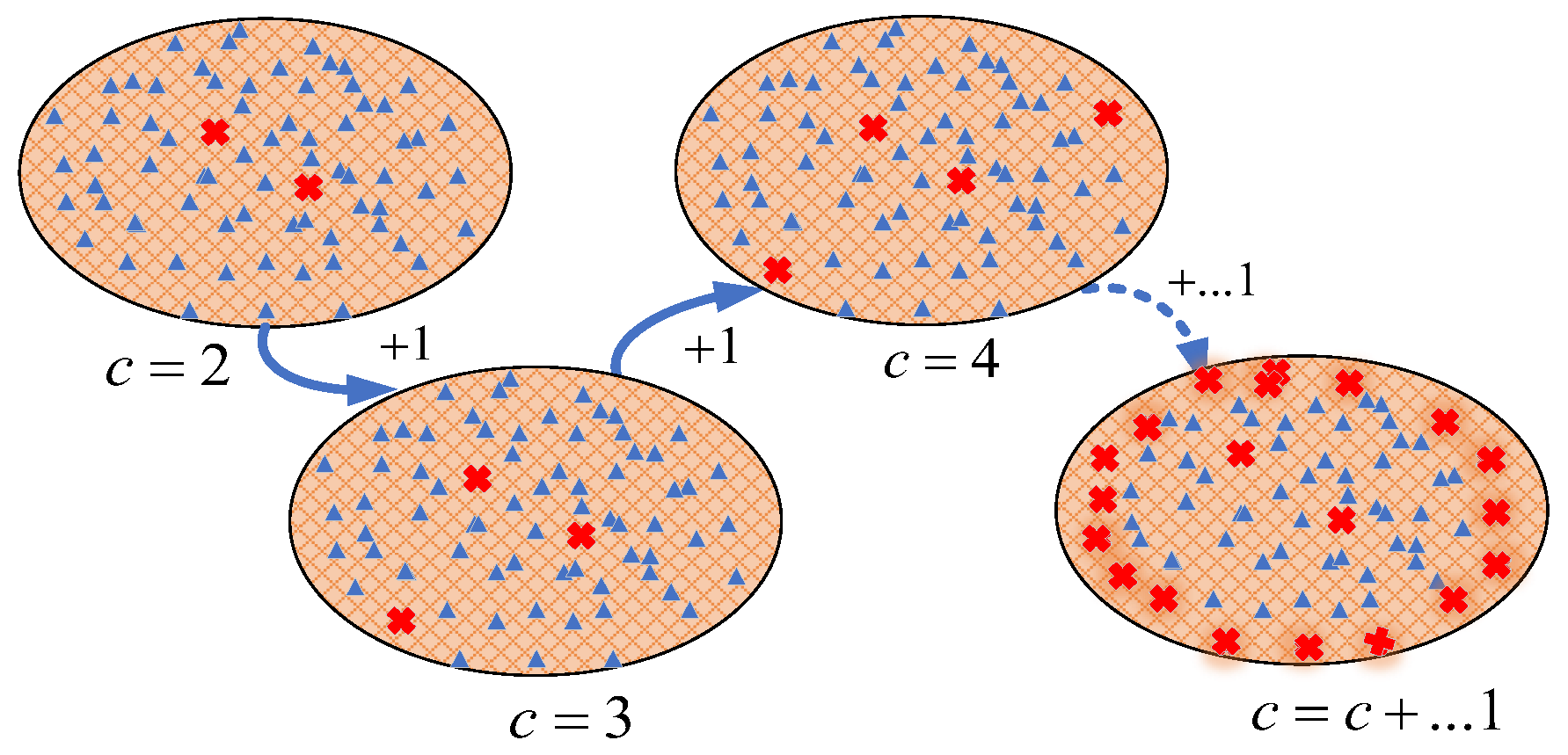
The new cluster center of the satisfactory FCM algorithm is to find the most dissimilar sample from the previous cluster center in the sample data as the new cluster center, that is, to find a sample in the sample set farthest from the cluster center to join the previous cluster. The center set $c_1~c_c$ constitutes a new cluster center set $c_1~c_{c+1}$, which will gradually “marginalize” the new cluster center. The problem of “marginalization” is illustrated in Figure 1. The clustering center gradually tends to follow the sample edge as the number of clusters increases.

To overcome the random initialization and poor new-cluster-center selection of the satisfactory FCM clustering algorithm, the k-means algorithm is introduced as a deterministic preprocessing step. Specifically, k-means provides stable initial cluster centers based on the data distribution, which eliminates the randomness of the initial membership matrix in FCM and ensures reproducible clustering results. This hybrid strategy also guides the selection of new cluster centers when the number of local models increases, thereby improving the determination of the optimal number of clusters.

To address the aforementioned problems of “marginalization”, selection of the number of local models, and random trials of the initial membership matrix of the satisfactory FCM clustering algorithm, this paper introduces the K-means clustering algorithm into the satisfactory FCM fuzzy clustering method and improves the satisfactory FCM. The algorithm’s new method of selecting cluster centers is improved, and the improvements are as follows:

(1)

Selection of initial membership matrix.

The K-means clustering algorithm is an algorithm that gathers $N$ sample objects into specified $c$ clusters according to the similarity between sample data. First, a $c$ cluster center needs to be initialized $\{c_1,c_2,c_3,\dots ,c_c\},1<c<N$. The initial number of clusters is specified as $c=2$ according to the satisfactory FCM algorithm. The Euclidean distance to each cluster center is then calculated for each sample data as follows:

$$\mathrm{dis}\left(\varphi (k,\alpha ),C_j\right)=\sqrt{{\displaystyle \sum _{t=1}^m{\left({\varphi }_t(k,\alpha )-C_{jt}\right)}^2}}$$

(14)

where $\varphi (k,\alpha )$ represents the $k\text{-}\mathrm{th}$ data sample $(1\le k\le N)$, $C_j$ indicates the $j\text{-}\mathrm{th}$ cluster center $(1\le j\le c)$, ${\varphi }_t(k,\alpha )$ denotes the $t\text{-}\mathrm{th}$ attribute of the sample data $k$$(1\le t\le m)$, and $C_{jt}$ signifies the $t\text{-}\mathrm{th}$ attribute of the cluster center $j$. The distance of each sample data to each cluster center is compared, and the sample data are assigned to the clusters of the nearest cluster center to form a $c$ cluster $\{s_1,s_2,s_3,\dots ,s_c\}$, $1<c<N$. Among these clusters, the cluster center is the mean value of all sample data in each dimension, which is calculated as follows:

$$C_t={\displaystyle \frac{{\displaystyle \sum _{\varphi (k,\alpha )\in S_l}\varphi (k,\alpha )}}{\left|S_l\right|}}$$

(15)

where $C_t$ represents the $l\text{-}\mathrm{th}$ cluster center $(1\le l\le c)$, $\left|S_l\right|$ indicates the number of sample data in the $l\text{-}\mathrm{th}$ cluster, and $\varphi (k,\alpha )$ denotes the $k\text{-}\mathrm{th}$ sample data in the $l\text{-}\mathrm{th}$ cluster $(1\le i\le \left|S_l\right|)$. In this manner, the initial clustering center of the satisfactory FCM algorithm can be obtained, and the problem of random trial and error of the initial membership degree matrix can be solved.

(2)

“Marginalization” and the number of local models.

To solve the problem of “marginalization” of the new cluster centers and the selection of the number of local models as determined by the satisfactory FCM clustering algorithm, this paper adopts the K-means algorithm to cluster and obtain new cluster centers. With the new cluster center as the initial clustering center, a new non-random membership matrix $\mathit{U}$ is calculated, and the satisfactory FCM algorithm is used to perform $c+1$ classification of the system again. A new cluster number is added according to the modeling accuracy index. These steps are repeated according to the performance index until a satisfactory result is obtained.

The objective function of the SKFCM hybrid clustering algorithm can be expressed as follows:

$$H(\mathit{U},\mathit{C})={\displaystyle {\displaystyle \sum _{i=1}^c}{\displaystyle \sum _{k=1}^N{\left({\mu }_{ik}\right)}^m}}{‖c_i-\varphi (k,\alpha )‖}^2$$

(16)

where ${\displaystyle \sum _{i=1}^c{\mu }_{ik}}=1$, $\mathit{U}={\left[{\mu }_{ik}\right]}_{c\times N}$ represents the membership degree matrix, $c$ is the number of clusters, $N$ is the number of samples, ${\mu }_{ik}$ is the membership of the $k\text{-}\mathrm{th}$ sample in the $i\text{-}\mathrm{th}$ cluster center, $C=\left[c_1,c_2,\dots ,c_c\right]$, $c_i$ is the $i\text{-}\mathrm{th}$ cluster center, and $\varphi (k,\alpha )$ is the $k\text{-}\mathrm{th}$ sample point, ${‖c_i-\varphi (k,\alpha )‖}^2$ represents the Euclidean distance between the cluster center $c_i$ and the sample point $\varphi (k,\alpha )$, and $m$ is a weighted index, generally taken as 2. Solving the minimum value problem of Equation (16), we can get:

$${\mu }_{i,k}={\displaystyle \frac{1}{{\displaystyle \sum _{j=1}^c{\left(\frac{\Vert \varphi (k,\alpha )-c_i\Vert }{\Vert \varphi (k,\alpha )-c_j\Vert }\right)}^{2/(m-1)}}}}$$

(17)

$$c_i={\displaystyle \frac{{\displaystyle \sum _{k=1}^N{\mu }_{ik}^m}\varphi (k,\alpha )}{{\displaystyle \sum _{k=1}^N{\mu }_{ik}^m}}}$$

(18)

The main procedural steps of the SKFCM hybrid clustering algorithm can be outlined as follows:

Step 1: Given a set of data samples $\varphi$, the initial number of clusters is set to $c=2$.

Step 2: The initial cluster center is determined according to Equations (14) and (15).

Step 3: The initial matrix $\mathit{U}$ is calculated using Equation (17).

Step 4: The initial cluster centers of the matrices obtained from Steps 3 and 2 are substituted into Equation (16) to calculate the accuracy index $H(\mathit{U},\mathit{C})$.

Step 5: Whether the convergence index satisfies $‖H_{l+1}-H_l‖\le \delta$, where $l$ is the number of iterations, and $\delta$ is the iteration accuracy. In general, $\delta =0.01$ can meet the accuracy requirements. $c$ cluster centers $c_i (i=1,2,\dots c)$ are then calculated.

Step 6: If the accuracy requirements are not met, then these steps are repeated until the given convergence index is met.

Step 7: Whether the accuracy index $H(\mathit{U},\mathit{C})$ meets the user accuracy requirements is determined. If not, then the number of clusters $c=c+1$ is increased. The process returns to step 2, and the steps are repeated until the accuracy requirements of the given user are met.

The steps of the SKFCM hybrid clustering algorithm are described in pseudocode as shown in

Table 1. Pseudocode of SKFCM hybrid clustering algorithm in this paper.

Step	Operate	Illustrate
1	Input data: Input signal $u(k)$, output signal $y(k)$, $k=1,\dots ,K$; fractional-order initial ${\alpha }^{(0)}$, model structure parameters $n_a,n_b$, calculation of $\varphi (k,\alpha )$, clustering parameters $m=2$, $\delta$, ${\alpha }_w<1$, optimization parameters $\Delta \alpha$, ${\lambda }_0$	Initialization
2	Given an initial number of clusters $c=2$, with weights $w_1=1$, $w_2={\alpha }_w$, respectively. Repeat: Calculate the minimum distance $d_j={\min }_i\left(w_i‖x_j-c_i‖\right)$ for each point; if $\max \left(d_j\right)<\delta$, exit the cluster; otherwise, use $\arg \max d_j$ as the new cluster center $c_{j+1}$, with weight $w_{j+1}=w_j\cdot {\alpha }_w$, $c=c+1$. Preliminary determination of cluster centers $C_0=\left[c_1,c_2,\dots ,c_c\right]$ for each variable.	SKFCM automatically determines the number of clusters.
3	The calculation of $C_0=\left[c_1,c_2,\dots ,c_c\right]$ is fast, but it suffers from marginalization. Regenerate clusters $C_1$ using K-means and update the cluster centers $C_0$ of each variable. Calculate the objective function value of the current cluster centers according to Equations (16) and (17). If the convergence condition is not met, update $C_j$ using Equation (18). If the convergence condition is met, output the cluster centers $C=\left[c_1,c_2,\cdots ,c_c\right]$ of each variable.	SKFCM automated refinement of cluster centers
4	Sparsely sample the center vector of each variable using a fixed step size; Combine all samples into a single combination, with each combination corresponding to a rule’s antecedent; Denoted by the total number of rules as n.	Determine the number of rules
5	Based on $\varphi (k,\alpha )$, construct the consequent matrix $\Phi$, with size $(K/2)\times \left(\left(n_a+n_b\right)\cdot n\right)$.	Successor matrix construction
6	Estimating consequent parameters $\theta :\theta ={\left({\Phi }^T\Phi \right)}^{-1}{\Phi }^T{Y}_{\mathrm{train}}$ using least-squares method.	Estimate consequent parameters
7	Optimize fractional-order $\alpha$: Calculate $J_{\alpha }^{\prime }$, $J_{\alpha }^{″}$ according to Equations (23) and (24). Iterate the value of $\alpha$ according to Equation (22).	LM algorithm for estimating fractional order
8	Calculation model output: Calculate $\widehat{y}(k)={\displaystyle \sum _{l=1}^n{\mu }_l}(k)\left(\Phi {\theta }_l\right)$ Calculate the objective function $J$ according to Equation (21). If $J$ decreases, then $\lambda \leftarrow 1.05$; otherwise $\lambda \leftarrow 0.95\lambda$.	Calculate the objective function
9	If $J<\epsilon$, then jump to 10; otherwise go to 6.	Termination judgment
10	The algorithm ends, outputting the consequent parameter $\theta$, fractional-order $\alpha$ and the model output $\widehat{y}$.	Program ended

.

3.2. Identification of Fractional-Order and Local Model Parameters

We propose to select the antecedent variable of the model as the fractional-order variable whose order is to be identified. This idea is then used to construct the fractional-order fuzzy multi-model of the system. The least-square algorithm and the LM algorithm are combined to interactively identify the local model parameters and the fractional order. First, the fractional-order antecedent variables are calculated by the GL calculus operator, whereas the scheduling function parameters are obtained by fuzzy division of the antecedent variables via the SKFCM algorithm. Second, the least-squares algorithm is used to identify the local model parameters of the system, and the local model is applied according to the scheduling function. The weighted combination obtains the global model of the system. Finally, whether the objective function (21) of the system reaches the minimum is evaluated. If it is not satisfied, then the Levenberg–Marquardt (LM) algorithm is used to iterate the fractional-order $\alpha$ until the objective function $J$ reaches the minimum, and the fractional-order and local model parameters are obtained.

The global model of the system can be expressed by (13) as:

$$\widehat{y}(k)=\phi {(k,\widehat{\alpha })}^T\widehat{\theta }$$

(19)

$$\widehat{\theta }={\left[a_{11} a_{12}\dots a_{1n_a} b_{11} b_{12}\dots b_{1n_b} a_{21} a_{22}\dots a_{2n_a} b_{21} b_{22}\dots b_{2n_b}\dots \dots a_{l1} a_{l2}\dots a_{l{\mathrm{n}}_a} b_{l1} b_{l2}\dots b_{l{\mathrm{n}}_b}\right]}^T$$

$$\begin{array}{l}\phi (k,\widehat{\alpha })=[-{\mu }_1{\Delta }^{\widehat{\alpha }}y(k-1)-{\mu }_1{\Delta }^{\widehat{\alpha }}y(k-2) \dots -{\mu }_1{\Delta }^{\widehat{\alpha }}y(k-n_a) \\ \hspace{1em}\hspace{1em}\hspace{1em}\hspace{1em} {\mu }_1{\Delta }^{\widehat{\alpha }}u(k-1) {\mu }_1{\Delta }^{\widehat{\alpha }}u(k-2)\dots {\mu }_1{\Delta }^{\widehat{\alpha }}u(k-n_b)\dots \\ \hspace{1em}\hspace{1em}\hspace{1em}\hspace{1em} -{\mu }_2{\Delta }^{\widehat{\alpha }}y(k-1)-{\mu }_2{\Delta }^{\widehat{\alpha }}y(k-2) \dots -{\mu }_2{\Delta }^{\widehat{\alpha }}y(k-n_a) \\ \hspace{1em}\hspace{1em}\hspace{1em}\hspace{1em} {\mu }_2{\Delta }^{\widehat{\alpha }}u(k-1) {\mu }_2{\Delta }^{\widehat{\alpha }}u(k-2)\dots {\mu }_2{\Delta }^{\widehat{\alpha }}u(k-n_b)\dots \dots \\ \hspace{1em}\hspace{1em}\hspace{1em}\hspace{1em} -{\mu }_l{\Delta }^{\widehat{\alpha }}y(k-1)-{\mu }_l{\Delta }^{\widehat{\alpha }}y(k-2) \dots -{\mu }_l{\Delta }^{\widehat{\alpha }}y(k-n_a) \\ \hspace{1em}\hspace{1em}\hspace{1em}\hspace{1em} {\mu }_l{\Delta }^{\widehat{\alpha }}u(k-1) {\mu }_l{\Delta }^{\widehat{\alpha }}u(k-2)\dots {\mu }_l{\Delta }^{\widehat{\alpha }}u(k-n_b) ]\end{array}$$

After determining the parameters of the system scheduling function, the scheduling function of each sample number in the data set $\varphi$ can be calculated by Equation (11). Hence, the identification problem of each local model parameter can be directly solved by the least-square algorithm. The local model parameters are solved once by the least-square algorithm:

$$\hat{\theta }={[\phi (k,\widehat{\alpha })\phi {(k,\widehat{\alpha })}^T]}^{-1}\phi (k,\widehat{\alpha }) y(k)$$

(20)

The objective function is:

$$\begin{array}{l}J={\displaystyle \frac{1}{K}}{\displaystyle {\displaystyle \sum _{k=1}^K}{\epsilon }^2}(k)={\displaystyle \frac{1}{K}}{\displaystyle {\displaystyle \sum _{k=1}^K}}[y(k)-\widehat{y}(k){]}^2\\ \hspace{1em}\hspace{1em}\hspace{1em}\hspace{1em}\hspace{1em}\hspace{1em}={\displaystyle \frac{1}{K}}{\displaystyle \sum _{k=1}^K}[y(k)-{\phi }^{\mathrm{T}}(k,\widehat{\alpha })\widehat{\theta }{]}^2\end{array}$$

(21)

where $K$ is the data length, and $\widehat{y}(k)$, $\widehat{\alpha }$, and $\widehat{\theta }$ are the estimated values of $y(k)$, $\alpha$, and $\theta$, respectively. The LM algorithm uses the following recurrence equation:

$$\left\{{\alpha }^{(i+1)}={\alpha }^{(i)}-{\left\{{\left[J_{\alpha }^{″}+\lambda I\right]}^{-1}{J}_{\alpha }^{\prime }\right\}}_{\widehat{\alpha }={\alpha }^{(i)}}\right.$$

(22)

The parameter update rule is based on the calculation of each parameter gradient $J^{\prime }$ and Hessian matrix $J^{″}$, where $\lambda$ is the convergent adjustment parameter.

$$\left\{\begin{array}{l}{J}_{\alpha }^{\prime }=-{\displaystyle \frac{2}{K}}{\left({\sigma }_{\hat{y}(k)/\alpha }\right)}^{\mathrm{T}}\left(y(k)-{\phi }^{\mathrm{T}}(k,\alpha )\theta \right)\\ J_{\alpha }^{″}={\displaystyle \frac{2}{K}}{\left({\sigma }_{\widehat{y}(k)/\alpha }\right)}^{\mathrm{T}}\left({\sigma }_{\widehat{y}(k)/\alpha }\right)\end{array}\right.$$

(23)

where ${\sigma }_{\widehat{y}(k)/\alpha }={\displaystyle \frac{\partial \widehat{y}(k)}{\partial \alpha }}$ is the output sensitivity, which is calculated by the following equation:

$${\sigma }_{\widehat{y}/\alpha }\approx {\displaystyle \frac{\widehat{y}(k,\alpha +\delta \alpha )-\widehat{y}(k,\alpha )}{\delta \alpha }}$$

(24)

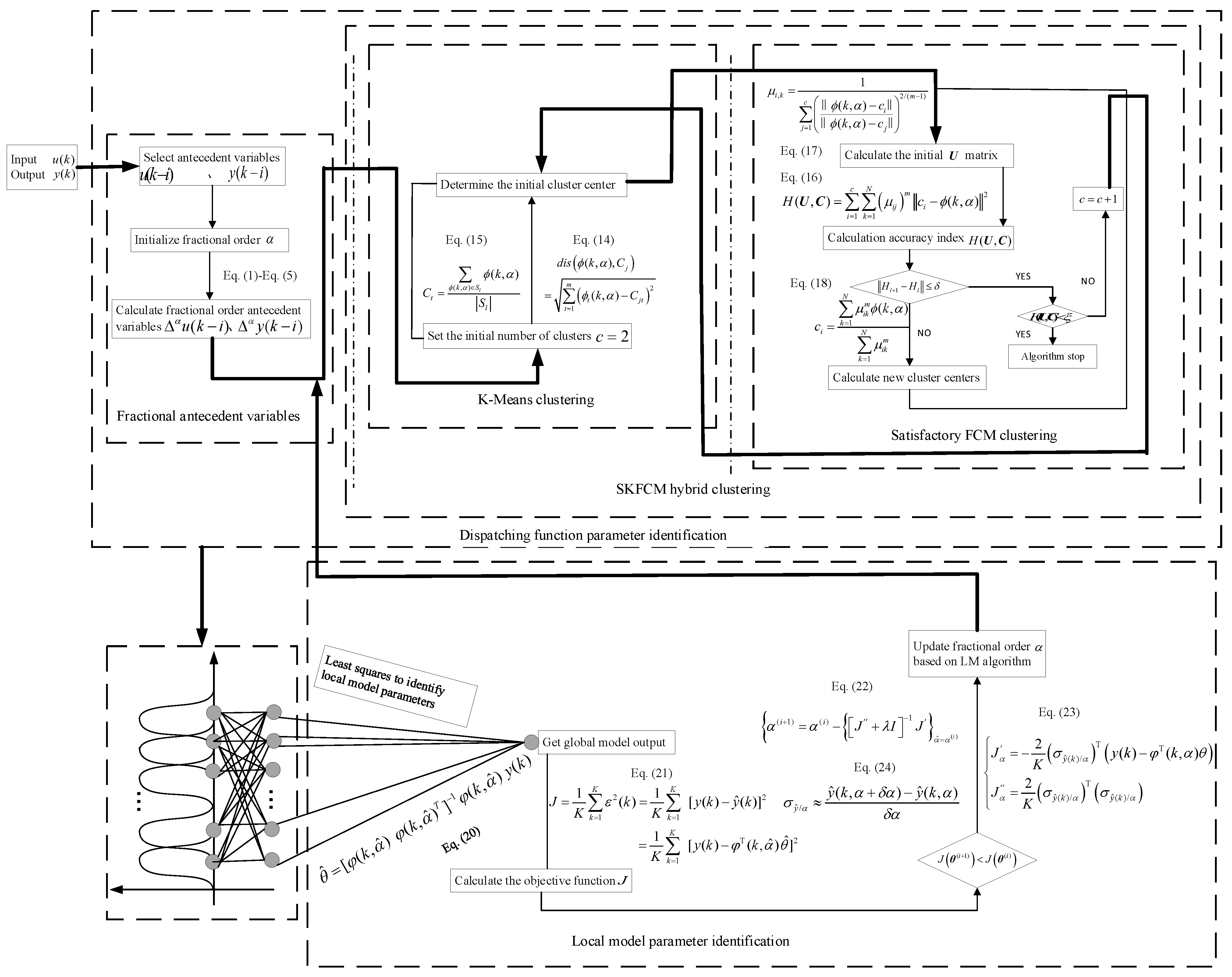
The input and output data collected by the system are divided into two parts: a training set and a test set. The training set is used to establish a fractional-order fuzzy multi-model of the system, whereas the test set is employed to verify the established model. The overall algorithm flow diagram of this chapter is as follows in Figure 2.

4. Simulation Examples

The proposed method is validated through two examples in this chapter. The first one is an academic case involving a strongly nonlinear and strongly coupled system. The second example is an experiment with a flexible manipulator. Reference [40] conducted a fractional-order H–W structure modeling, but its linear block and nonlinear block structure parameters did not have an effective method to determine. Therefore, the fractional-order fuzzy multi-model proposed herein is used to model and identify it. The simulation results are compared with those of the method used in [40] to verify the effectiveness of the method proposed in this paper.

4.1. Academic Calculation Example

A fractional-order system of a strongly nonlinear and strongly coupled system is constructed as follows. There is a strong coupling between its output items.

$$\begin{array}{l}y(k)=a_1{\Delta }^{\alpha }(y(k-1))+a_2{\Delta }^{\alpha }y(k-2){\Delta }^{\alpha }y(k-1)+\dots \\ \hspace{1em}\hspace{1em} b_1{\Delta }^{\alpha }u(k-1)+b_2{\Delta }^{\alpha }u(k-2)+\dots \\ \hspace{1em}\hspace{1em} p_2{b}_1{\Delta }^{\alpha }{u}^2(k-1)+p_2{b}_2{\Delta }^{\alpha }{u}^2(k-2)\end{array}$$

(25)

where

$[a_1 a_2]=\left[-0.1 -0.2\right]$; $[b_1 b_2]=\left[0.4 0.2\right]$;

$[p_1 p_2]=\left[1 0.5\right]$; $\alpha =0.6$.

The fractional-order fuzzy multi-model is then implemented to approximate the system.

$$\begin{array}{l}\varphi (k,\alpha )=\{{\Delta }^{\widehat{\alpha }}y(k-1),{\Delta }^{\widehat{\alpha }}y(k-2),{\Delta }^{\widehat{\alpha }}y(k-3),\dots \\ \hspace{1em}\hspace{1em}\hspace{1em}\hspace{1em}{\Delta }^{\widehat{\alpha }}u(k-1),{\Delta }^{\widehat{\alpha }}u(k-2),{\Delta }^{\widehat{\alpha }}u(k-3)\}\end{array}$$

(26)

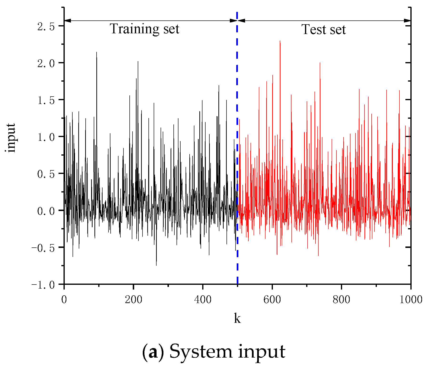
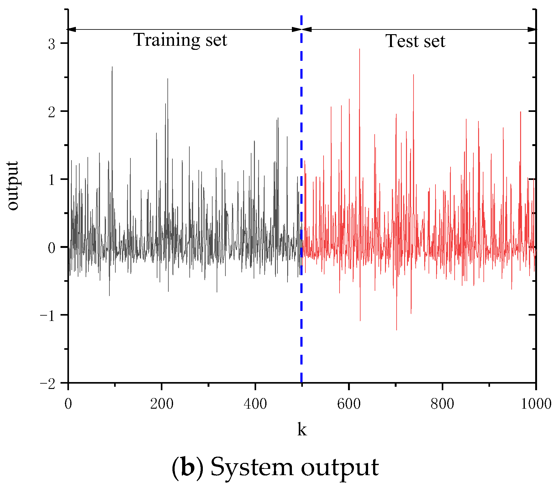
is selected as the input variable of the antecedent. The $u(k)$ input uses a continuous excitation signal with a mean value of 0 and a variance of 1. At the same time, Gaussian white noise with a mean of 0 and a variance of 0.01 is added. The number of collected data signals is 1000. The input and output signals are shown in Figure 3. The measured data set contains two parts: the first 500 are used to establish a fractional-order fuzzy multi-model, and the remaining 500 are utilized for test verification. The noise is Gaussian white noise with a mean value of 0 and a variance of 0.01.

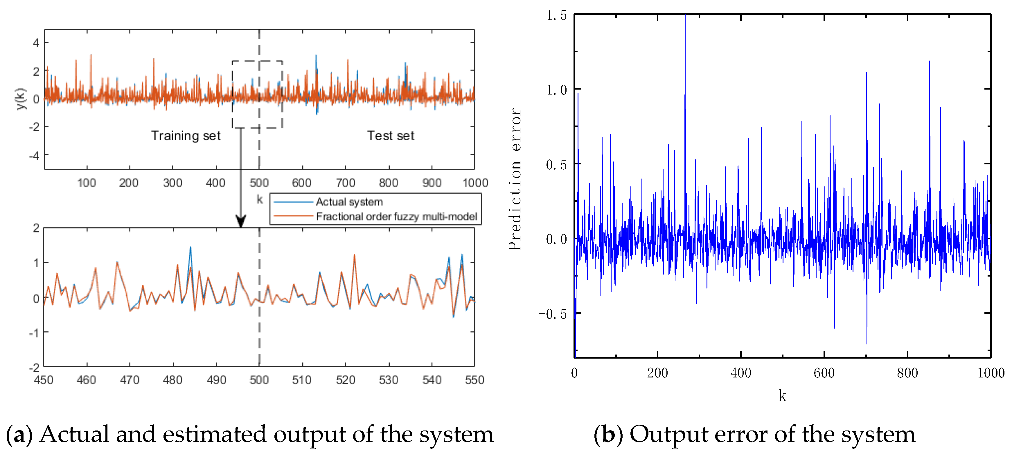
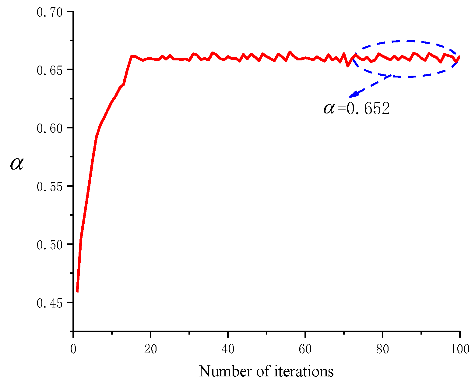
The fractional-order fuzzy multi-model proposed in this paper is applied to model the system using 6 local models. The parameters of the local models are summarized in

Table 2. Parameters of the local model.

	${\mathit{a}}_{\mathit{l}1}$	${\mathit{a}}_{\mathit{l}2}$	${\mathit{a}}_{\mathit{l}3}$	${\mathit{b}}_{\mathit{l}1}$	${\mathit{b}}_{\mathit{l}2}$	${\mathit{b}}_{\mathit{l}3}$
$R^1$	−0.2484	−0.1504	0.03824	0.19111	0.04012	−0.029
$R^2$	−0.0418	0.36294	0.18225	0.29545	0.11232	−0.1075
$R^3$	−0.2803	−0.1547	0.01724	0.56058	0.33757	−0.0717
$R^4$	0.05426	0.07174	0.04499	0.75302	0.55598	0.03532
$R^5$	0.01119	0.12247	0.05323	0.04407	−0.1632	−0.0597
$R^6$	0.32357	0.17154	0.07235	0.21819	0.1539	0.00902

. The actual system after modeling, the output of the estimated system, and the prediction error are shown in Figure 4. The fractional-order identification of the system is 0.652, as shown in Figure 5. A comparison of the estimated output and the actual output, as well as partially amplifying the difference between them, reveals that the actual output data overlap with and basically fit the estimated output data.

By combining the parameters of the local model in Table 2, the system can be represented by six fractional-order fuzzy rules, and the overall fuzzy model of the system is represented as follows:

$$\begin{array}{l}{R}^1: if \varphi (k,\alpha ) is F_1,\\ \hspace{1em}\hspace{1em}then y_1(k)=-0.2484{\Delta }^{0.652}y(k-1)-0.1504{\Delta }^{0.652}y(k-2)+0.03824{\Delta }^{0.652}y(k-3)\\ \hspace{1em}\hspace{1em}\hspace{1em}\hspace{1em}\hspace{1em}\hspace{1em}\hspace{1em} +0.19111{\Delta }^{0.652}u(k-1)+0.04012{\Delta }^{0.652}u(k-2)-0.029{\Delta }^{0.652}u(k-3)\end{array}$$

$$\begin{array}{l}\hspace{1em}\hspace{1em}{R}^2: if \varphi (k,\alpha ) is F_2,\\ \hspace{1em}\hspace{1em}\hspace{1em}\hspace{1em}then y_2(k)=-0.0418{\Delta }^{ 0.652}y(k-1)+0.36294{\Delta }^{0.652}y(k-2)+0.18225{\Delta }^{0.652}y(k-3)\\ \hspace{1em}\hspace{1em}\hspace{1em}\hspace{1em}\hspace{1em}\hspace{1em}\hspace{1em}\hspace{1em}\hspace{1em} +0.29545{\Delta }^{0.652}u(k-1)+0.11232{\Delta }^{0.652}u(k-2)-0.1075{\Delta }^{0.652}u(k-3)\end{array}$$

$$\begin{array}{l}\hspace{1em}\hspace{1em}{R}^3: if \varphi (k,\alpha ) is F_3,\\ \hspace{1em}\hspace{1em}\hspace{1em}\hspace{1em}then y_3(k)=-0.2803{\Delta }^{ 0.652}y(k-1)-0.1547{\Delta }^{0.652}y(k-2)+0.01724{\Delta }^{0.652}y(k-3)\\ \hspace{1em}\hspace{1em}\hspace{1em}\hspace{1em}\hspace{1em}\hspace{1em}\hspace{1em}\hspace{1em}\hspace{1em} +0.56058{\Delta }^{0.652}u(k-1)+0.33757{\Delta }^{0.652}u(k-2)-0.0717{\Delta }^{0.652}u(k-3)\end{array}$$

$$\begin{array}{l}\hspace{1em}\hspace{1em}{R}^4: if \varphi (k,\alpha ) is F_4,\\ \hspace{1em}\hspace{1em}\hspace{1em}\hspace{1em}then y_4(k)=0.05426{\Delta }^{ 0.652}y(k-1)+0.07174{\Delta }^{0.652}y(k-2)+0.04499{\Delta }^{0.652}y(k-3)\\ \hspace{1em}\hspace{1em}\hspace{1em}\hspace{1em}\hspace{1em}\hspace{1em}\hspace{1em}\hspace{1em}\hspace{1em} +0.75302{\Delta }^{0.652}u(k-1)+0.55598{\Delta }^{0.652}u(k-2)+0.03532{\Delta }^{0.652}u(k-3)\end{array}$$

$$\begin{array}{l}\hspace{1em}\hspace{1em}{R}^5: if \varphi (k,\alpha ) is F_5,\\ \hspace{1em}\hspace{1em}\hspace{1em}\hspace{1em}then y_5(k)=0.01119{\Delta }^{ 0.652}y(k-1)+0.12247{\Delta }^{0.652}y(k-2)+0.05323{\Delta }^{0.652}y(k-3)\\ \hspace{1em}\hspace{1em}\hspace{1em}\hspace{1em}\hspace{1em}\hspace{1em}\hspace{1em}\hspace{1em}\hspace{1em} +0.04407{\Delta }^{0.652}u(k-1)-0.1632{\Delta }^{0.652}u(k-2)-0.0597{\Delta }^{0.652}u(k-3)\end{array}$$

$$\begin{array}{l}\hspace{1em}\hspace{1em}{R}^6: if \varphi (k,\alpha )is F_6,\\ \hspace{1em}\hspace{1em}\hspace{1em}\hspace{1em}then y_6(k)=0.32357{\Delta }^{ 0.652}y(k-1)+0.17154{\Delta }^{0.652}y(k-2)+0.07235{\Delta }^{0.652}y(k-3)\\ \hspace{1em}\hspace{1em}\hspace{1em}\hspace{1em}\hspace{1em}\hspace{1em}\hspace{1em}\hspace{1em}\hspace{1em} +0.21819{\Delta }^{0.652}u(k-1)+0.1539{\Delta }^{0.652}u(k-2)+0.00902{\Delta }^{0.652}u(k-3)\end{array}$$

4.2. Robotic Arm Calculation Example

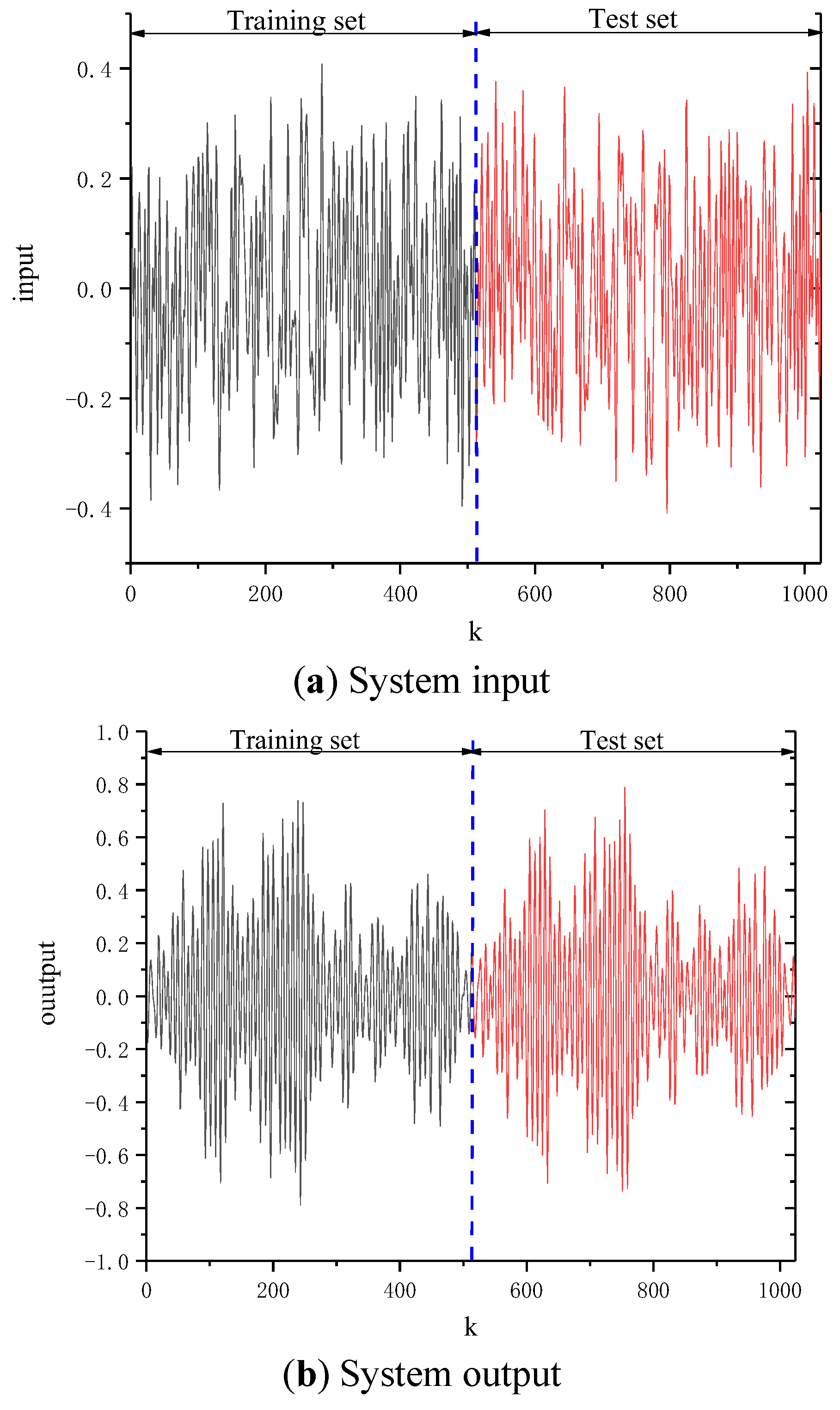
Further verification of the proposed method is carried out on the flexible robotic arm benchmark dataset obtained from the DAISY database [41] (a system identification database). The system is composed of an arm mounted on a motor, with the reaction torque of the structure on the ground as the input and the acceleration of the flexible arm as the output. A total of 1024 samples are available in the measured dataset, which are partitioned into a training set (first part) and a test set (second part). The noise is Gaussian white noise with zero mean and variance 0.01. Modeling and identification are performed using the fractional-order fuzzy multi-model proposed herein, and the simulation outcomes are compared with those achieved by the method in [40]. The input and output signals of the flexible robot arm are depicted in Figure 6. References [42,43] also performed NLARX and NARMAX structural modeling of this dataset. The present work establishes a fractional-order fuzzy multi-model of the flexible robot arm.

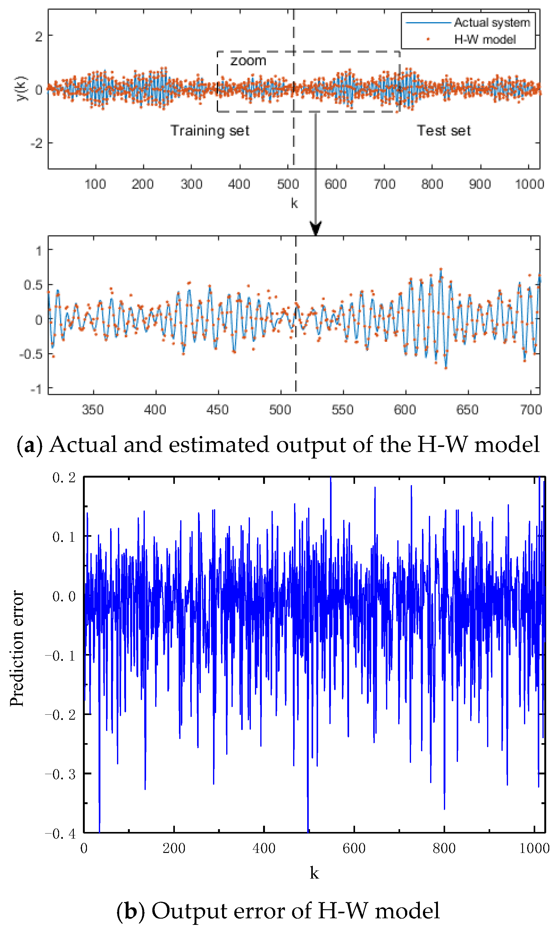
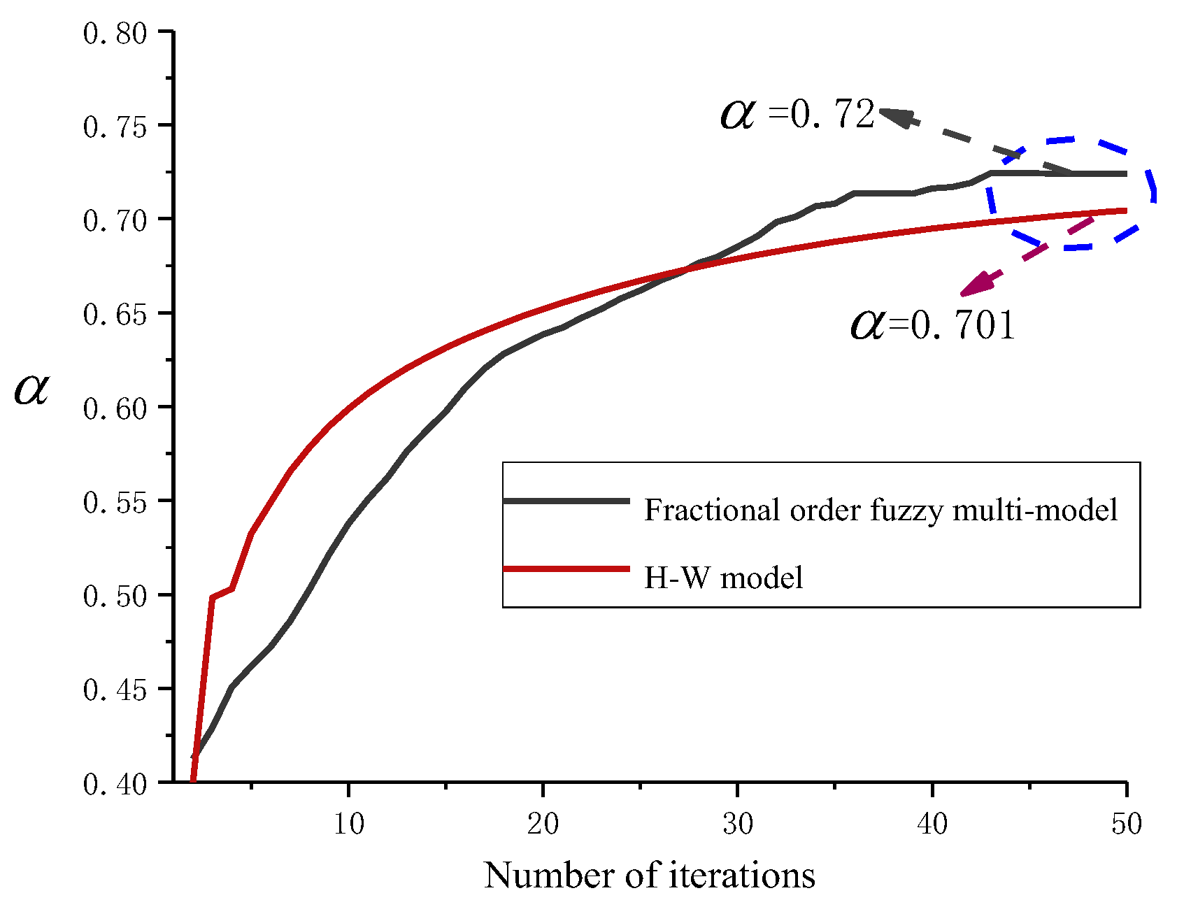
The H–W structure reported in the literature [40] is used to establish the H–W model of the system. The model structure is selected according to the literature [40]. As shown in Figure 7a, if the actual output of the system and the output of the H–W model are enlarged, then the actual output data can be clearly seen to overlap the estimated output data, and the degree of fit is relatively high. Figure 7b represents the prediction error. The error ranges from −0.4 to 0.2, and the error is relatively large. The system fractional order identified by the H-W model is 0.701, as shown in Figure 8.

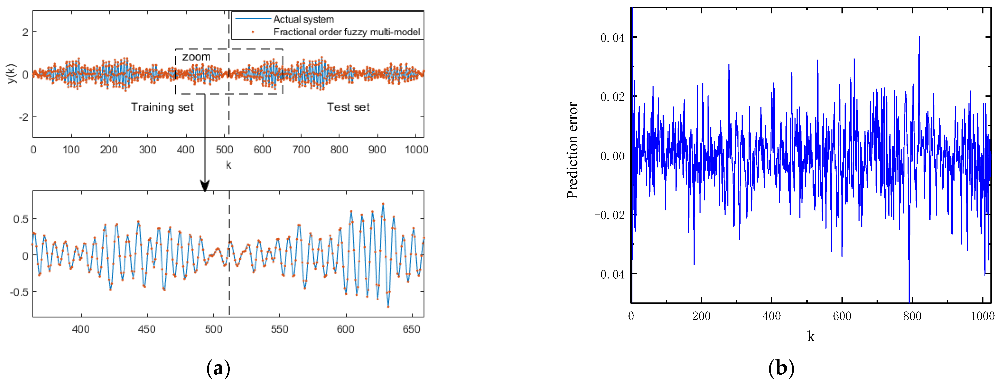
The system is modeled by the fractional-order fuzzy multi-model proposed herein. The number of local models is 18, and the parameters of the local models are summarized in

Table 3. Parameters of the local model.

	${\mathit{a}}_{\mathit{l}1}$	${\mathit{a}}_{\mathit{l}2}$	${\mathit{a}}_{\mathit{l}3}$	${\mathit{b}}_{\mathit{l}1}$	${\mathit{b}}_{\mathit{l}2}$	${\mathit{b}}_{\mathit{l}3}$	${\mathit{b}}_{\mathit{l}4}$	${\mathit{b}}_{\mathit{l}5}$
$R^1$	0.09450	0.14373	0.11314	0.00664	0.03187	0.04534	0.03720	0.01230
$R^2$	0.02460	0.00145	0.02290	0.00786	0.00284	0.00729	0.01243	0.00698
$R^3$	0.17801	0.23929	0.17020	0.03156	0.05565	0.06145	0.04447	0.01209
$R^4$	0.04183	0.07478	0.06235	0.02168	0.01814	0.00451	0.02699	0.03026
$R^5$	0.04390	0.11296	0.11608	0.01395	0.00100	0.02125	0.03108	0.02286
$R^6$	0.06943	0.02724	0.02870	0.01797	0.01311	0.00076	0.01426	0.01924
$R^7$	0.02525	0.10136	0.11439	0.03986	0.02471	0.01461	0.04592	0.04451
$R^8$	0.17466	0.21437	0.13890	0.03768	0.05963	0.05662	0.03139	0.00149
$R^9$	0.07986	0.08579	0.04444	0.00848	0.02279	0.02776	0.01867	0.00061
$R^{10}$	0.12896	0.19475	0.15230	0.00996	0.03475	0.04972	0.04378	0.01873
$R^{11}$	0.02302	0.05513	0.05769	0.02426	0.01881	0.00003	0.01544	0.01533
$R^{12}$	0.09756	0.05317	0.01604	0.04011	0.03517	0.00660	0.02556	0.03999
$R^{13}$	0.01778	0.07233	0.08102	0.03432	0.02398	0.00895	0.03814	0.04016
$R^{14}$	0.09151	0.10952	0.06802	0.03090	0.02505	0.00271	0.01775	0.02325
$R^{15}$	0.12242	0.10849	0.03843	0.04165	0.05004	0.02792	0.00773	0.03223
$R^{16}$	−0.05866	−0.03058	0.01550	0.00022	−0.00915	−0.01069	−0.00513	−0.00079
$R^{17}$	0.11235	0.12502	0.06955	−0.02794	−0.02384	−0.00538	0.01319	0.02128
$R^{18}$	0.07704	0.07848	0.03673	−0.01821	−0.01389	−0.00175	0.00905	0.01264

. As shown in Figure 8, the identified system fractional order is 0.72. The output of the actual system, the estimated system, and the prediction error after modeling are shown in Figure 9. In Figure 9a, the estimated output and the actual output are partially enlarged, and the actual output data can be clearly seen to overlap with and completely fit the estimated output data. The prediction error shown in Figure 9b ranges from −0.04 to 0.02. Compared with the error of the H–W model, the accuracy of the model introduced herein is improved by nearly 10-fold.

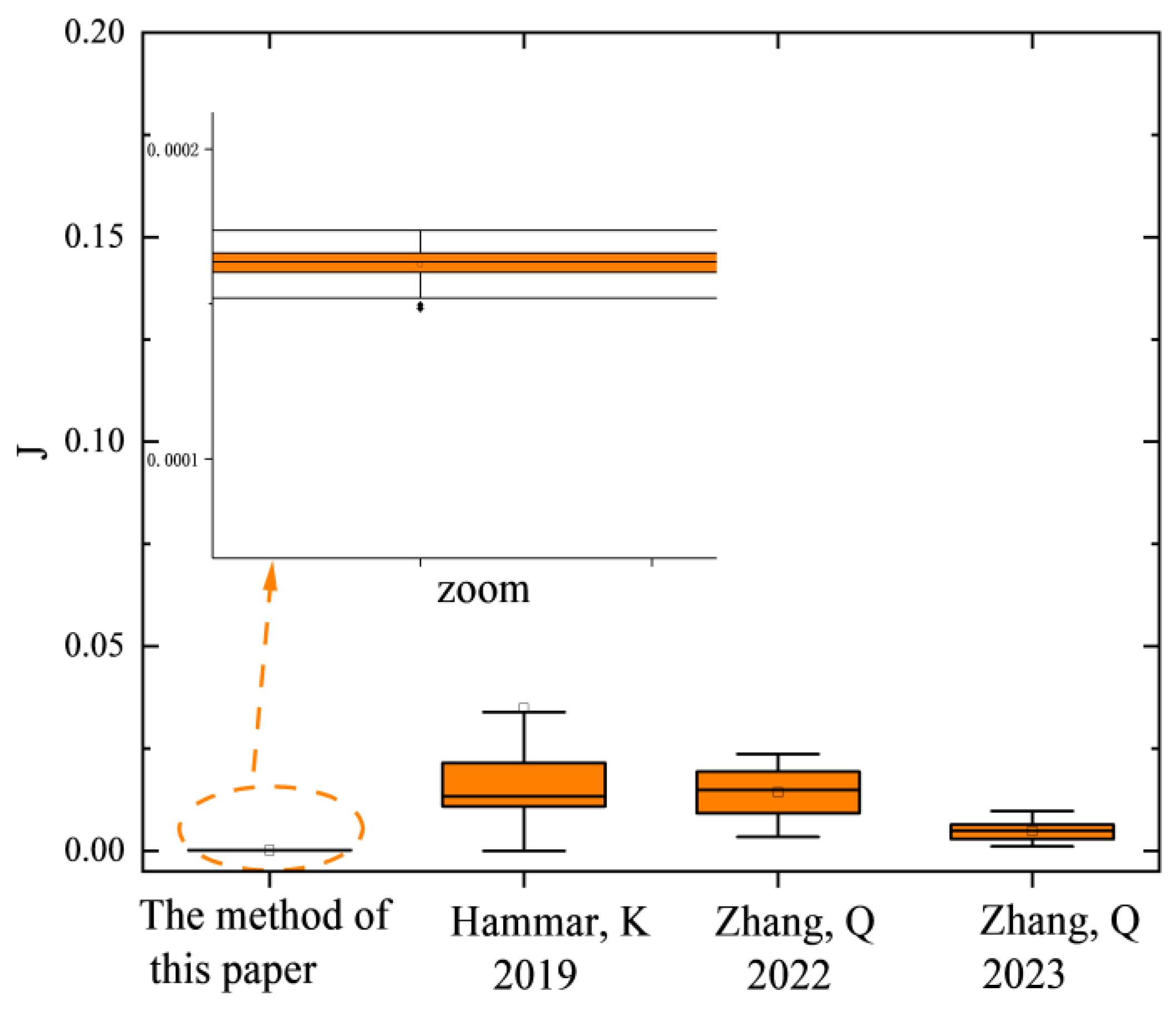
The objective function error and mean square error $J$ of the model in [4,40,44] are compared with the fractional-order fuzzy multi-model proposed in this paper (Figure 10). Given that the error of the fractional-order fuzzy multi-model is small, the fitting degree is high, and the mean square error $J$ is small, and can be partially enlarged. Therefore, the modeling effect is substantially improved.

For the research on the modeling method of this manipulator system, the author has completed a lot of work before. In references [4,40,44], Zhang, Q et al., Hammar, K et al., and Zhang, Q et al. have studied various fractional-order parameter modeling methods. We compared the identification effects of the non-parametric modeling method proposed in this paper, as shown in

Table 4. Comparison of the error range of the robot arm estimation with the literature.

Method	[40]	[44]	[4]	The Method of This Paper
Error range	[−0.2, 0.2]	[−0.15, 0.15]	[−0.1, 0.1]	[−0.04, 0.04]

. It can be seen that for the data of the same manipulator system, the fuzzy multi-model method proposed in this paper has smaller modeling errors and more accurate results.

5. Conclusions

A new method for modeling and identifying fractional-order fuzzy multi-model systems is proposed herein. The input and output framework is adopted on the basis of the decomposition–synthesis principle. The SKFCM hybrid clustering algorithm is proposed, and the satisfactory FCM algorithm is improved to solve the problem of accurately determining the number of local models and selecting the initial cluster center. The antecedent is selected as a fractional-order variable of unknown order, and the LM algorithm is combined with the least square algorithm to interactively solve the problems of local model parameters and fractional order. A robotic arm calculation example is used to compare the method proposed in this paper with the method reported in the literature. Theoretical analyses and simulations proved that the fractional-order fuzzy multi-model method introduced in this study has a good fit and a high accuracy. How to control the established fractional fuzzy model is the author’s next research objective.

References

1. Das, D.; Taralova, I.; Loiseau, J.J.; Slavov, T.; Pandey, M. Frequency Domain Identification of a 1-DoF and 3-DoF Fractional-Order Duffing System Using Grünwald–Letnikov Characterization. Fractal Fract. 2025, 9, 581. [Google Scholar] [CrossRef]
2. Victor, S.; Valério, D. Special section on fractional differentiation and its applications: Modeling and system identification. Annu. Rev. Control. 2025, 61, 101019. [Google Scholar] [CrossRef]
3. Bingi, K.; Rajanarayan Prusty, B.; Pal Singh, A. A review on fractional-order modelling and control of robotic manipulators. Fractal Fract. 2023, 7, 77. [Google Scholar] [CrossRef]
4. Zhang, Q.; Wang, H.; Liu, C. Hybrid identification method for fractional-order nonlinear systems based on the multi-innovation principle. Appl. Intell. 2023, 53, 15711–15726. [Google Scholar]
5. Ao, Y.; Liu, Y.-C.; Laghrouche, S.; Candusso, D. Dynamic fractional-order model of proton exchange membrane fuel cell system for sustainability improvement. Sustainability 2024, 16, 2939. [Google Scholar] [CrossRef]
6. Zhang, Q.; Wang, H.; Liu, C.; An, Y. Establishment and identification of MIMO fractional Hammerstein model with colored noise for PEMFC system. Chaos Solitons Fractals 2024, 180, 114502. [Google Scholar]
7. Yang, B.; Wang, D.; Sun, X.; Chen, S.; Wang, X. Offline order recognition for state estimation of Lithium-ion battery using fractional-order model. Appl. Energy 2023, 341, 120977. [Google Scholar] [CrossRef]
8. Wang, Y.; Ding, J.; Tu, T. An improved unscented Kalman filter for SOC estimation of lithium-ion batteries based on fractional-order model. Ionics 2025, 31, 4281–4298. [Google Scholar] [CrossRef]
9. De La Morena, J.; Redrejo, D.; Ramos, F.; Feliu, V.; Vázquez, A.S. Fractional-order modeling and control of hydrogel-based soft pneumatic bending actuators. In Proceedings of the 2024 IEEE/RSJ International Conference on Intelligent Robots and Systems (IROS), Abu Dhabi, United Arab Emirates, 14–18 October 2024; pp. 11362–11367. [Google Scholar]
10. Antunes, J.; Piteau, P.; Delaune, X.; Lagrange, R.; Panunzio, D. A parsimonious identification approach in the frequency-domain for experimental fractional systems of unknown order. In Proceedings of the NODYCON 2023, Rome, Italy, 18–22 June 2023. [Google Scholar]
11. Yuan, M.; Xu, W.; Liu, F.; Wang, L.; Lu, Y. Identification method for a fractional-order system in terms of equivalent dynamic properties. Chaos Interdiscip. J. Nonlinear Sci. 2024, 34, 073119. [Google Scholar] [CrossRef]
12. Duhé, J.-F.; Victor, S.; Melchior, P.; Abdelmoumen, Y.; Roubertie, F. Recursive system identification of continuous-time fractional systems for all parameter estimation. IEEE Trans. Control. Syst. Technol. 2024, 32, 2037–2049. [Google Scholar] [CrossRef]
13. Hu, C.; Ji, Y.; Ma, C. Joint two-stage multi-innovation recursive least-squares parameter and fractional-order estimation algorithm for the fractional-order input nonlinear output-error autoregressive model. Int. J. Adapt. Control Signal Process. 2023, 37, 1650–1670. [Google Scholar] [CrossRef]
14. Zhang, Y.; Zhang, X.; Ding, F. Hierarchical estimation method for fractional-order systems based on the auxiliary model. Appl. Math. Comput. 2026, 512, 129749. [Google Scholar] [CrossRef]
15. Gao, Z. Modulating function-based system identification for a fractional-order system with a time delay involving measurement noise using least-squares method. Int. J. Syst. Sci. 2017, 48, 1460–1471. [Google Scholar] [CrossRef]
16. Zhang, L.; Wang, X.; Chen, M.; Yu, F.; Li, M. A fractional-order model of lithium-ion batteries and multi-domain parameter identification method. J. Energy Storage 2022, 50, 104595. [Google Scholar] [CrossRef]
17. Yuan, L.; Yang, Q.; Zeng, C. Chaos detection and parameter identification in fractional-order chaotic systems with delay. Nonlinear Dyn. 2013, 73, 439–448. [Google Scholar] [CrossRef]
18. Xie, B.; Ge, F. Parameters and order identification of fractional-order epidemiological systems by Lévy-PSO and its application for the spread of COVID-19. Chaos Solitons Fractals 2023, 168, 113163. [Google Scholar] [CrossRef]
19. Zong, T.; Li, J.; Lu, G. Identification of fractional-order Wiener-Hammerstein systems based on adaptively fuzzy PSO and data filtering technique. Appl. Intell. 2023, 53, 14085–14101. [Google Scholar] [CrossRef]
20. Qaraad, M.; Amjad, S.; Hussein, N.K.; Mirjalili, S.; Elhosseini, M.A. An innovative time-varying particle swarm-based Salp algorithm for intrusion detection system and large-scale global optimization problems. Artif. Intell. Rev. 2023, 56, 8325–8392. [Google Scholar] [CrossRef]
21. Wang, J.; Si, Q.; Chen, J.; Zhang, Y. Simultaneous identification of time-delay parameter and fractional-order in nonlinear fractional delay differential equation. Appl. Math. Lett. 2023, 145, 108740. [Google Scholar] [CrossRef]
22. Liu, C.; Wang, H.; Zhang, Q.; Ahemaide, M. Identification of fractional-order non–homogeneous Hammerstein-Wiener MISO continuous systems. Mech. Syst. Signal Process. 2023, 197, 110400. [Google Scholar]
23. Wang, Z.; Liang, S.; Chen, B.; Sun, H. Identification of fractional-order time delay system with measurement noise using variable period integration operational matrix. Mech. Syst. Signal Process. 2025, 223, 111930. [Google Scholar] [CrossRef]
24. Ding, J.; Xu, S.; Li, Z. Fractional-order Learning Methods for Nonlinear System Identification Based on Fuzzy Neural Network. Int. J. Numer. Anal. Model. 2023, 20, 709–723. [Google Scholar] [CrossRef]
25. Liu, Y.; Liu, Y.; Shao, Q.; Wang, R.; Lv, Y. A novel neuro-fuzzy learning algorithm for first-order Takagi–Sugeno fuzzy model: Caputo fractional-order gradient descent method. Int. J. Fuzzy Syst. 2024, 26, 2616–2631. [Google Scholar] [CrossRef]
26. Dhahri, S.; Naifar, O.; Ben Alaia, E. Actuator and sensor fault estimation for T–S fuzzy fractional-order systems based on adaptive and sliding mode observers. Meas. Control 2025, 58, 1245–1262. [Google Scholar] [CrossRef]
27. Zennir, Y.; Guechi, E.; Bendib, R. Robust fractional multi-controller design of inverted pendulum system. In Proceedings of the 2016 20th International Conference on System Theory, Control and Computing (ICSTCC), Sinaia, Romania, 13–15 October 2016. [Google Scholar]
28. Wang, C.; Tan, H.; Hu, J.; Zhou, D. RL algorithm: An approximation algorithm for fractal signals based on fractional calculus. Fractals 2021, 29, 2150243. [Google Scholar] [CrossRef]
29. Fahad, H.M.; Fernandez, A. Operational calculus for Caputo fractional calculus with respect to functions and the associated fractional differential equations. Appl. Math. Comput. 2021, 409, 126400. [Google Scholar] [CrossRef]
30. Wang, X.; Luo, D.; Zhu, Q. Ulam-Hyers stability of caputo type fuzzy fractional differential equations with time-delays. Chaos Solitons Fractals 2022, 156, 111822. [Google Scholar] [CrossRef]
31. Leyden, K.; Goodwine, B. Fractional-order system identification for health monitoring. Nonlinear Dyn. 2018, 92, 1317–1334. [Google Scholar] [CrossRef]
32. Lang, H.; Ji, Y. Joint State and Parameter Estimation for the Fractional-Order Wiener State Space System Based on the Kalman Filtering. Int. J. Adapt. Control Signal Process. 2025, 39, 1712–1730. [Google Scholar] [CrossRef]
33. Yasin, Y.; Demir, G.; Riaz, M.; Aslam, M.; Pamucar, D. A systematic investigation of multi-attributive border approximation area comparison approach with Gaussian membership function for optimizing water quality. Environ. Dev. Sustain. 2024, 1–34. [Google Scholar] [CrossRef]
34. Azimi Amrei, S.M.; Miar Naimi, H. Designing an analog CMOS fuzzy logic controller for the inverted pendulum with a novel triangular membership function. Sci. Iran. 2019, 26, 1736–1748. [Google Scholar]
35. Rahim, R. Comparative analysis of membership function on Mamdani fuzzy inference system for decision making. J. Phys. Conf. Ser. 2017, 930, 012029. [Google Scholar]
36. Verma, H.; Verma, D.; Tiwari, P.K. A population based hybrid FCM-PSO algorithm for clustering analysis and segmentation of brain image. Expert Syst. Appl. 2021, 167, 114121. [Google Scholar] [CrossRef]
37. Bas, E.; Egrioglu, E. A fuzzy regression functions approach based on Gustafson-Kessel clustering algorithm. Inf. Sci. 2022, 592, 206–214. [Google Scholar] [CrossRef]
38. Xue, Z. Multi-Model Modeling and Control Based on Local Model Network. Doctoral Dissertation, Shanghai Jiaotong University, Shanghai, China, 2005. [Google Scholar]
39. Ikotun, A.M.; Ezugwu, A.E.; Abualigah, L.; Abuhaija, B.; Heming, J. K-means clustering algorithms: A comprehensive review, variants analysis, and advances in the era of big data. Inf. Sci. 2023, 622, 178–210. [Google Scholar] [CrossRef]
40. Hammar, K.; Djamah, T.; Bettayeb, M. Nonlinear system identification using fractional Hammerstein–Wiener models. Nonlinear Dyn. 2019, 98, 2327–2338. [Google Scholar] [CrossRef]
41. De Moor, B.; De Gersem, P.; De Schutter, B.; Favoreel, W. DAISY: A database for identification of systems. J. A 1997, 38, 4–5. [Google Scholar]
42. Schoukens, J.; Suykens, J.; Ljung, L. Wiener-hammerstein benchmark. In Proceedings of the 15th IFAC Symposium on System Identification, St. Malo, France, 6–8 July 2009. [Google Scholar]
43. Ugalde, H.M.R.; Carmona, J.-C.; Reyes-Reyes, J.; Alvarado, V.M.; Mantilla, J. Computational cost improvement of neural network models in black box nonlinear system identification. Neurocomputing 2015, 166, 96–108. [Google Scholar] [CrossRef]
44. Zhang, Q.; Wang, H.; Liu, C. MILM hybrid identification method of fractional-order neural-fuzzy Hammerstein model. Nonlinear Dyn. 2022, 108, 2337–2351. [Google Scholar] [CrossRef]
Figure 1. “Marginalization” problem.
Fractalfract 10 00362 g001
Figure 2. Block diagram of the overall algorithm flow.
Fractalfract 10 00362 g002
Figure 3. System input and output.
Fractalfract 10 00362 g003aFractalfract 10 00362 g003b
Figure 4. System actual, estimated output, and prediction error.
Fractalfract 10 00362 g004
Figure 5. Estimated value of fractional order α .
Fractalfract 10 00362 g005
Figure 6. System input and output.
Fractalfract 10 00362 g006
Figure 7. H-W model system actual, estimated output, and prediction error.
Fractalfract 10 00362 g007
Figure 8. Estimated value of fractional order α .
Fractalfract 10 00362 g008
Figure 9. System actual, estimated output, and prediction error of fractional-order fuzzy multi-model. (a) Actual and estimated output of fractional-order fuzzy multi-model; (b) Output error of fractional-order fuzzy multi-model.
Fractalfract 10 00362 g009
Figure 10. The objective function J of the four modeling methods, [4,40,44].
Fractalfract 10 00362 g010