Figure 1.
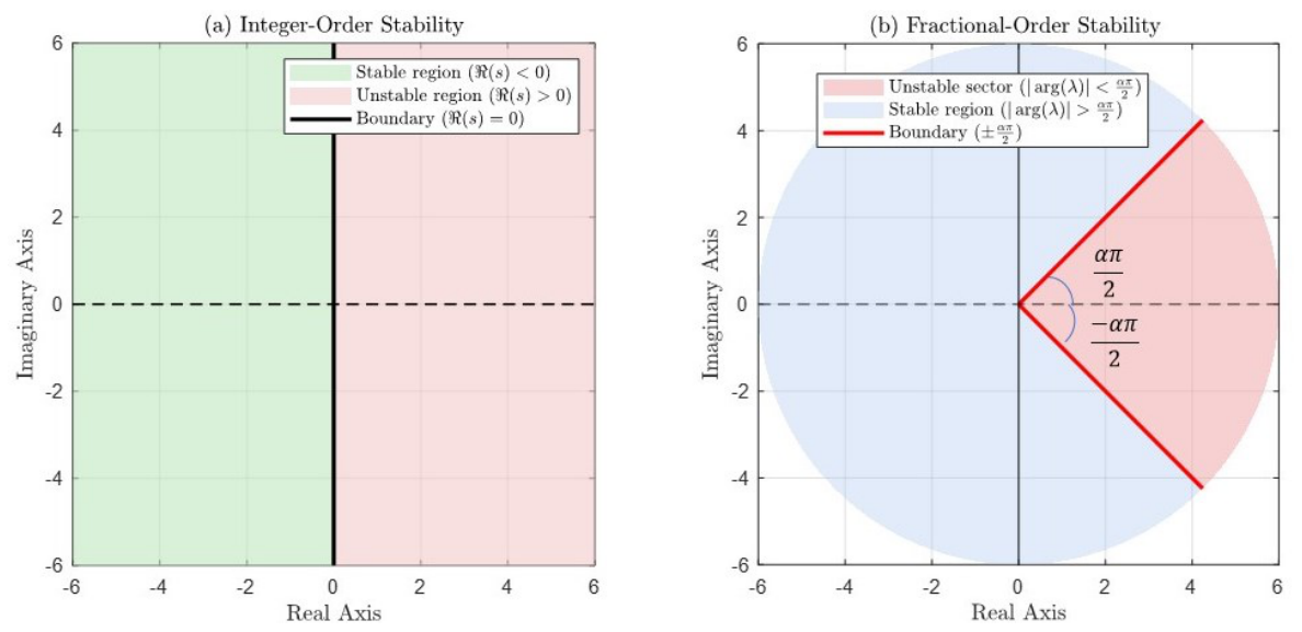
Comparison of stability regions for integer-order and fractional-order systems. (a) The integer-order system is stable in the left half-plane defined by , with the imaginary axis representing the stability boundary. (b) The fractional-order system exhibits a sector-shaped stability region, where instability is confined to and stability is achieved outside this sector. This illustrates the transformation of the classical half−plane stability condition into an angle-dependent criterion. For , the fractional−order system reduces to the classical integer-order case, and therefore, the stability regions of (a) and (b) coincide.
Figure 1.
Comparison of stability regions for integer-order and fractional-order systems. (a) The integer-order system is stable in the left half-plane defined by , with the imaginary axis representing the stability boundary. (b) The fractional-order system exhibits a sector-shaped stability region, where instability is confined to and stability is achieved outside this sector. This illustrates the transformation of the classical half−plane stability condition into an angle-dependent criterion. For , the fractional−order system reduces to the classical integer-order case, and therefore, the stability regions of (a) and (b) coincide.
Figure 2.
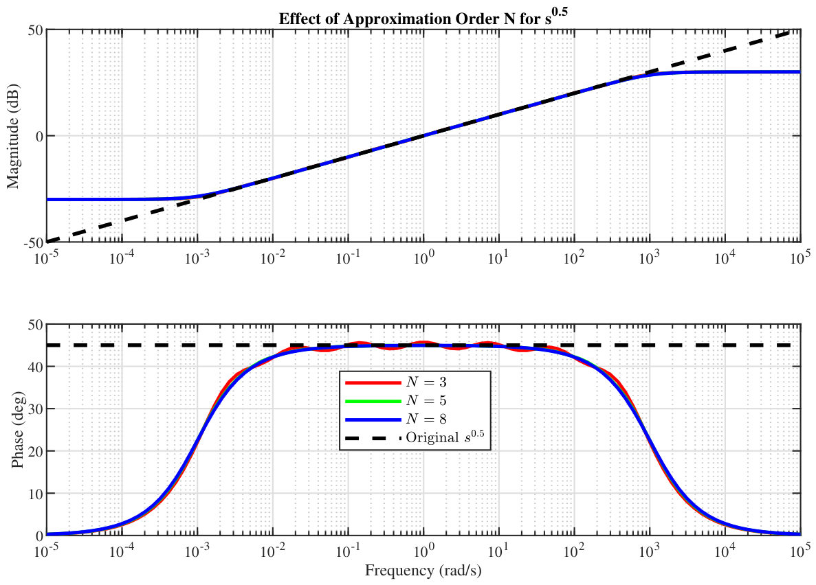
Bode magnitude and phase responses of the third-, fifth-, and eighth-order Oustaloup recursive approximation (ORA) models of over the frequency band rad/s.
Figure 2.
Bode magnitude and phase responses of the third-, fifth-, and eighth-order Oustaloup recursive approximation (ORA) models of over the frequency band rad/s.
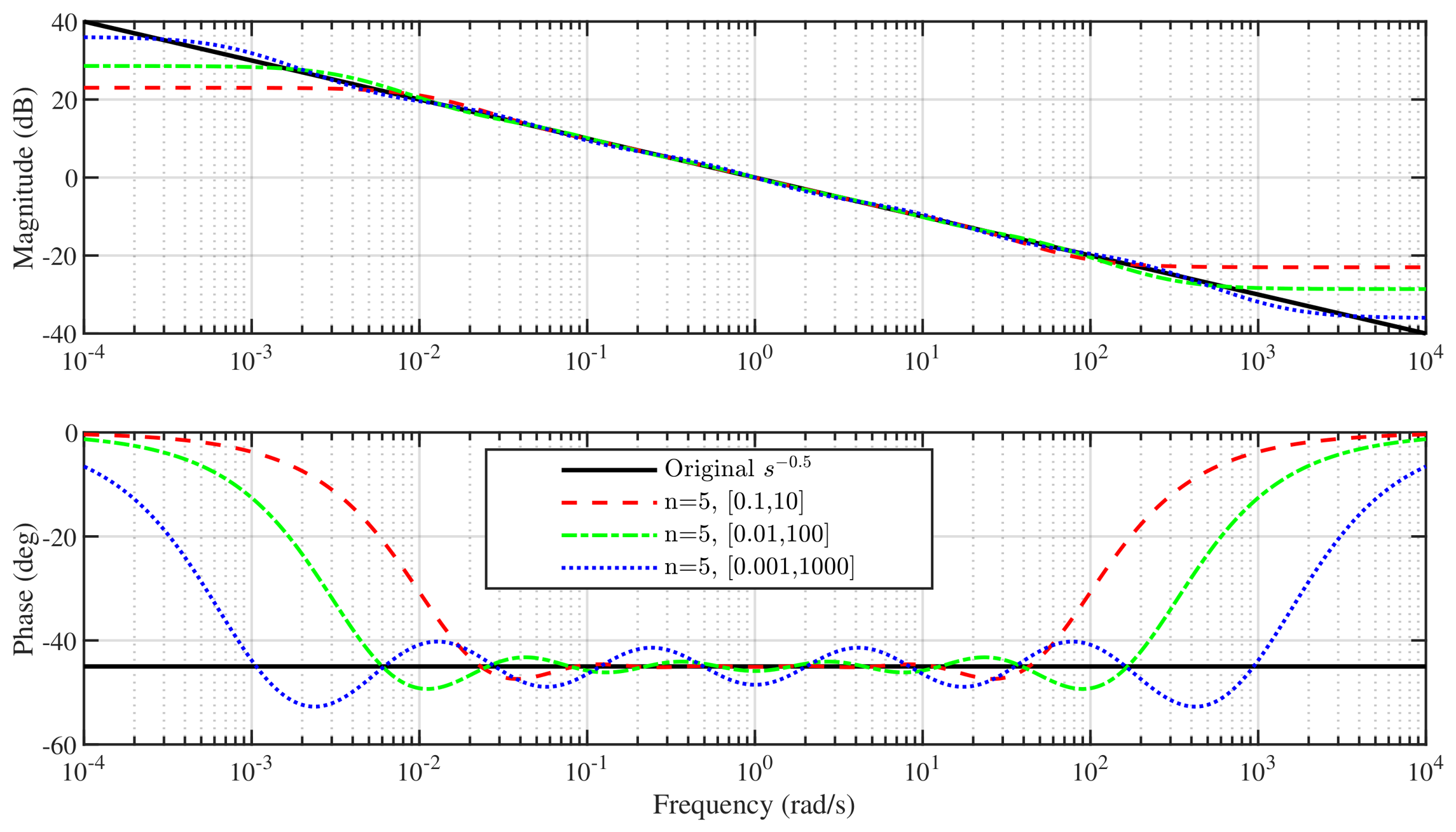
Figure 3.
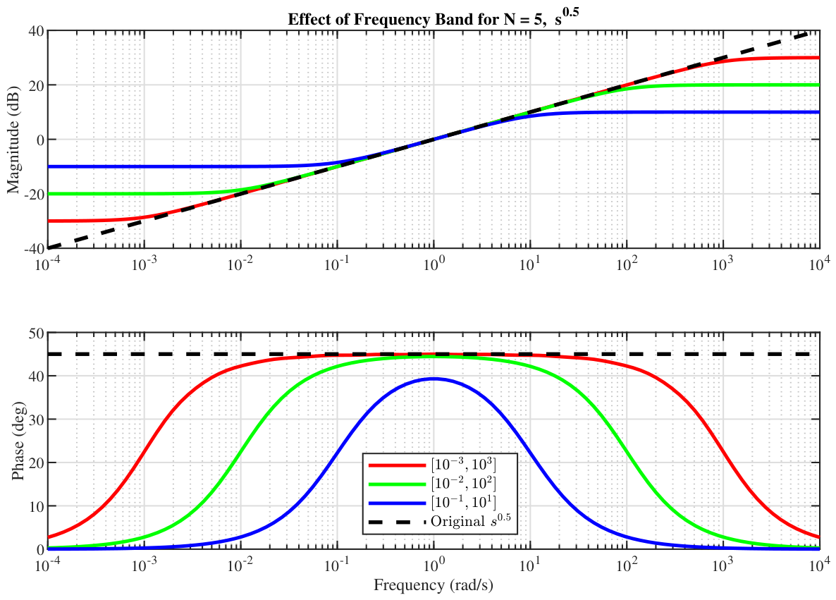
Bode magnitude and phase responses of the ORA models of for different frequency bands , , and rad/s with fixed approximation order .
Figure 3.
Bode magnitude and phase responses of the ORA models of for different frequency bands , , and rad/s with fixed approximation order .
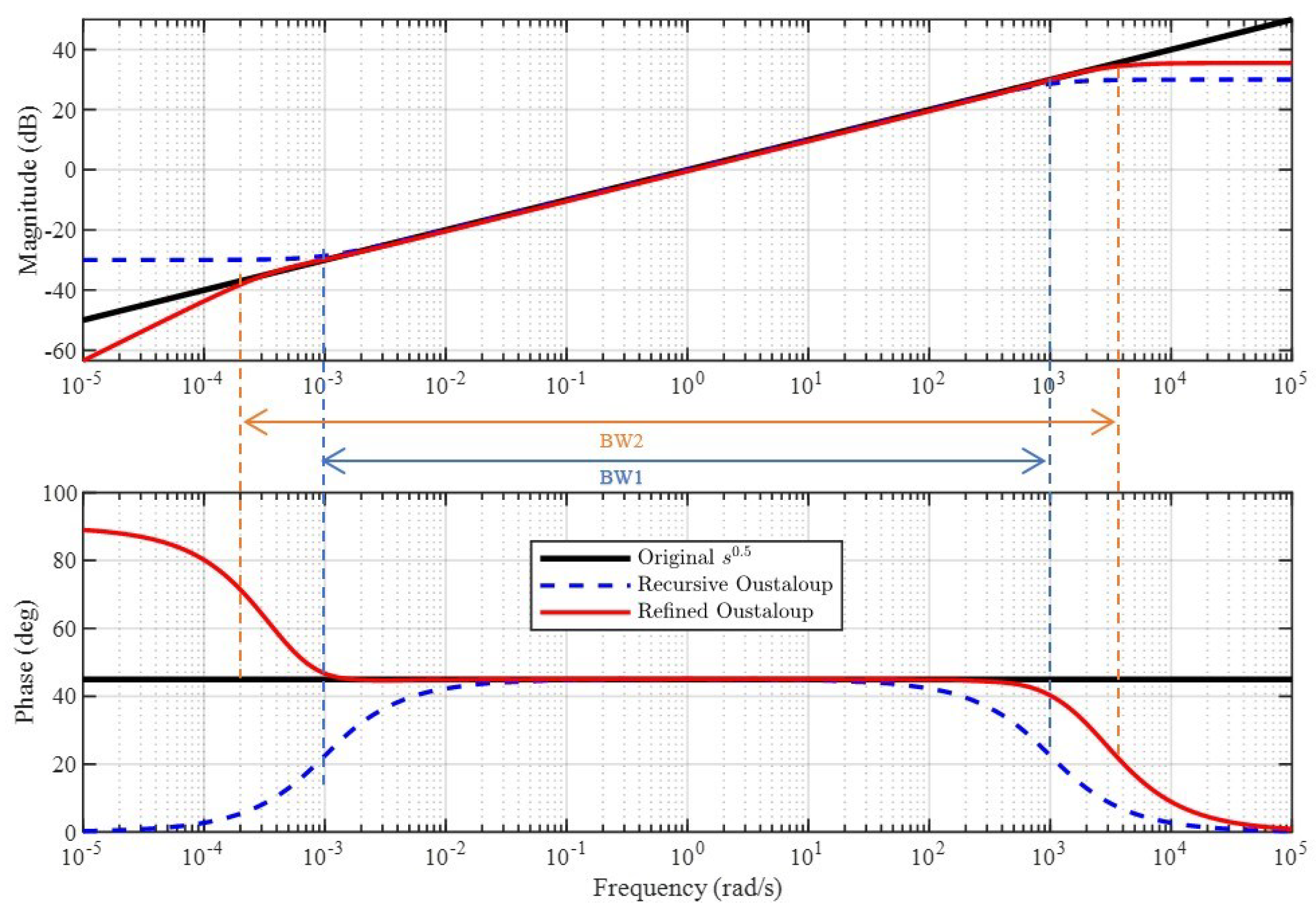
Figure 4.
Comparison of Bode magnitude and phase responses for the fifth-order ORA and ROA models of over the frequency band rad/s.
Figure 4.
Comparison of Bode magnitude and phase responses for the fifth-order ORA and ROA models of over the frequency band rad/s.
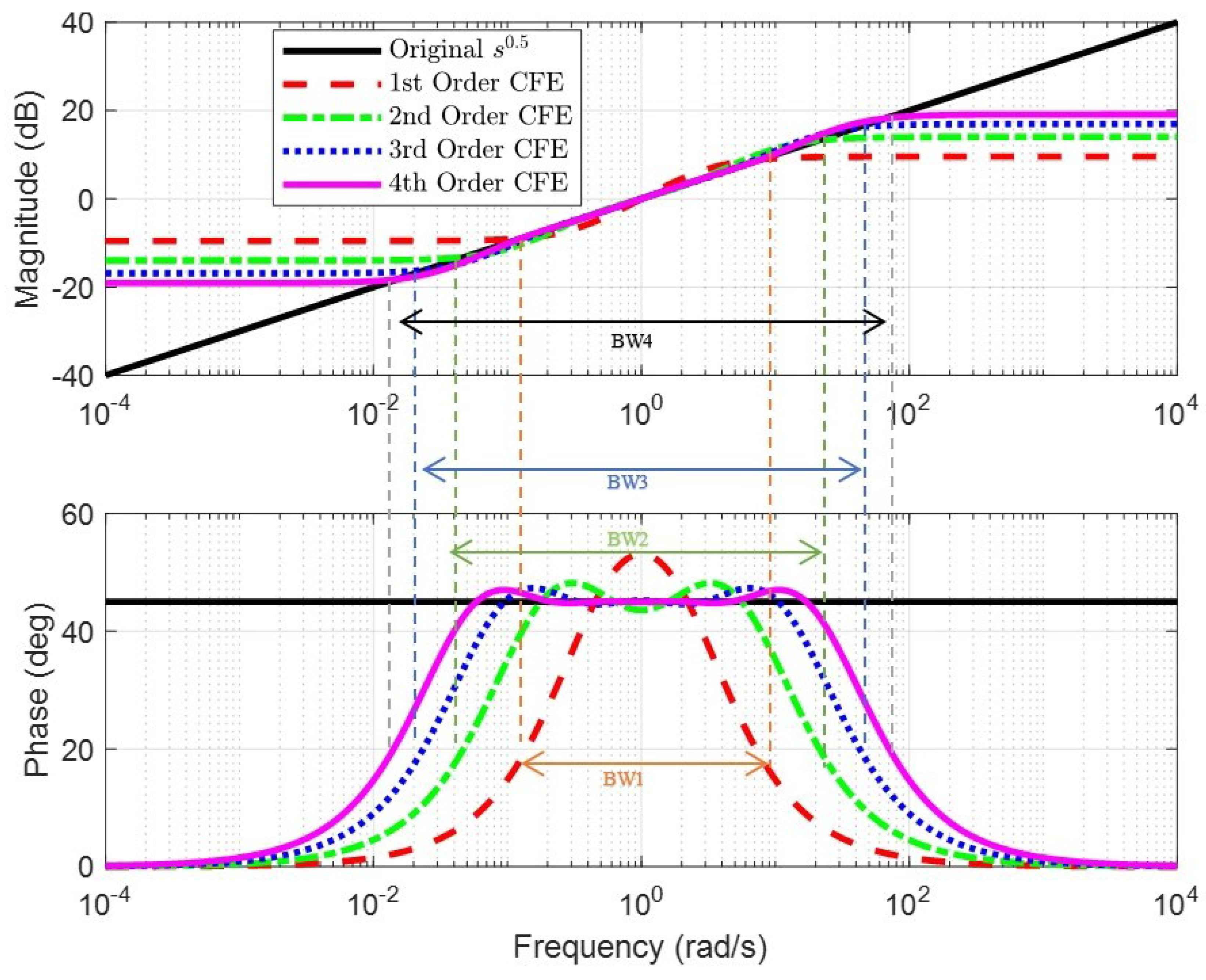
Figure 5.
Bode magnitude and phase responses of first- to fourth-order CFE approximation models of .
Figure 5.
Bode magnitude and phase responses of first- to fourth-order CFE approximation models of .
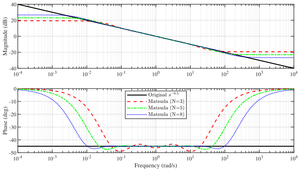
Figure 6.
Bode magnitude and phase responses of the third-, fifth-, and eighth-order Matsuda approximation models of over the frequency range rad/s.
Figure 6.
Bode magnitude and phase responses of the third-, fifth-, and eighth-order Matsuda approximation models of over the frequency range rad/s.
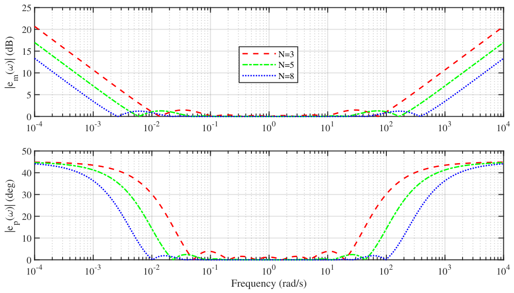
Figure 7.
Magnitude and phase errors of the third-, fifth-, and eighth-order Matsuda approximation models of .
Figure 7.
Magnitude and phase errors of the third-, fifth-, and eighth-order Matsuda approximation models of .
Figure 8.
Bode magnitude and phase responses of the Matsuda approximation models of for different frequency bands , , and rad/s with fixed approximation order .
Figure 8.
Bode magnitude and phase responses of the Matsuda approximation models of for different frequency bands , , and rad/s with fixed approximation order .
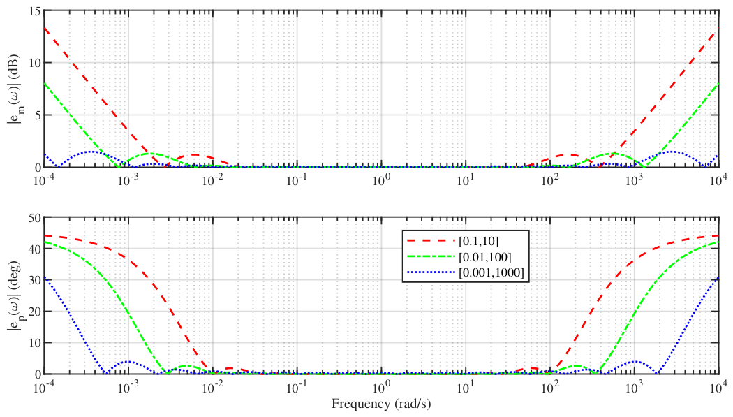
Figure 9.
Magnitude and phase errors of the Matsuda approximation models of for different frequency bands , , and rad/s with fixed approximation order .
Figure 9.
Magnitude and phase errors of the Matsuda approximation models of for different frequency bands , , and rad/s with fixed approximation order .
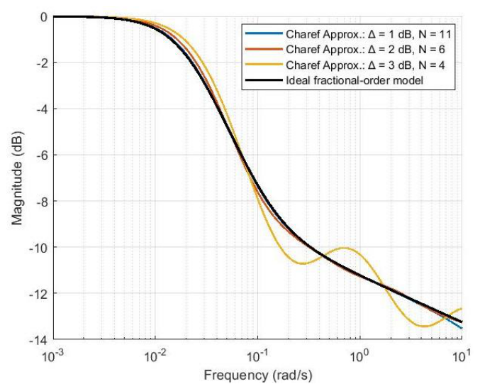
Figure 10.
Magnitude response of the Charef approximation for different error tolerances
dB for transfer function stated in Equation (
67).
Figure 10.
Magnitude response of the Charef approximation for different error tolerances
dB for transfer function stated in Equation (
67).
Figure 11.
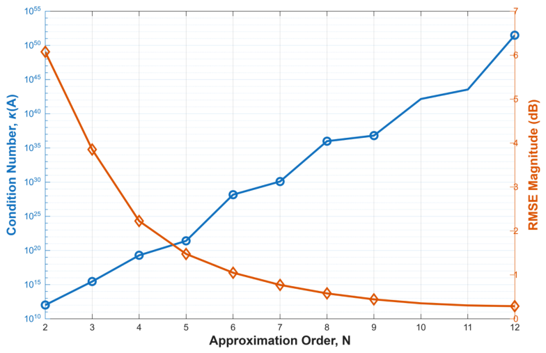
M-SBL Accuracy and Numerical Conditioning Trade-off for .
Figure 11.
M-SBL Accuracy and Numerical Conditioning Trade-off for .
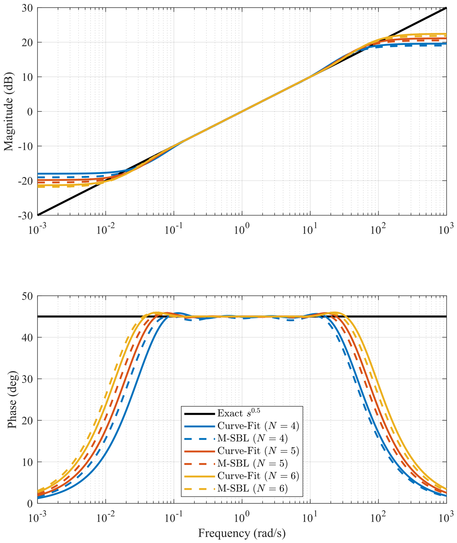
Figure 12.
Bode plot comparison between the true fractional-order system and its M-SBL and curve-fitting approximations for orders to 6. The magnitude and phase responses highlight the accuracy and frequency-domain behavior of each approximation method relative to the true model. As the approximation order increases, the M-SBL approximations better align with the true system, especially within the frequency range .
Figure 12.
Bode plot comparison between the true fractional-order system and its M-SBL and curve-fitting approximations for orders to 6. The magnitude and phase responses highlight the accuracy and frequency-domain behavior of each approximation method relative to the true model. As the approximation order increases, the M-SBL approximations better align with the true system, especially within the frequency range .
Figure 13.
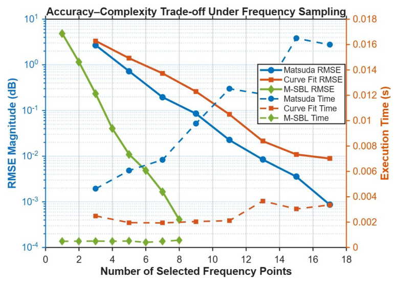
Influence of frequency-point selection on approximation accuracy and computational cost for the fractional operator using Matsuda, curve-fitting, and M-SBL methods.
Figure 13.
Influence of frequency-point selection on approximation accuracy and computational cost for the fractional operator using Matsuda, curve-fitting, and M-SBL methods.
Figure 14.
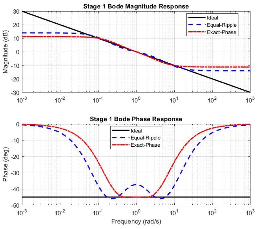
Bode plot of two biquad approximations for a 0.5 order integrator: the exact-phase design (red) vs. an equal-ripple design (blue). The exact-phase biquad achieves a near-constant phase over its band, whereas the ripple-optimized design shows larger phase variation. Both have similar dB/decade gain slopes, but the exact-phase filter has smoother phase.
Figure 14.
Bode plot of two biquad approximations for a 0.5 order integrator: the exact-phase design (red) vs. an equal-ripple design (blue). The exact-phase biquad achieves a near-constant phase over its band, whereas the ripple-optimized design shows larger phase variation. Both have similar dB/decade gain slopes, but the exact-phase filter has smoother phase.
Figure 15.
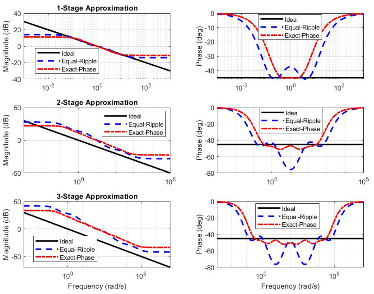
Bode plots of equal-ripple and exact-phase approximations for using different cascade stages. The plots compare the accuracy of the magnitude and phase responses of each approximation method against the ideal fractional-order behavior.
Figure 15.
Bode plots of equal-ripple and exact-phase approximations for using different cascade stages. The plots compare the accuracy of the magnitude and phase responses of each approximation method against the ideal fractional-order behavior.
Figure 16.
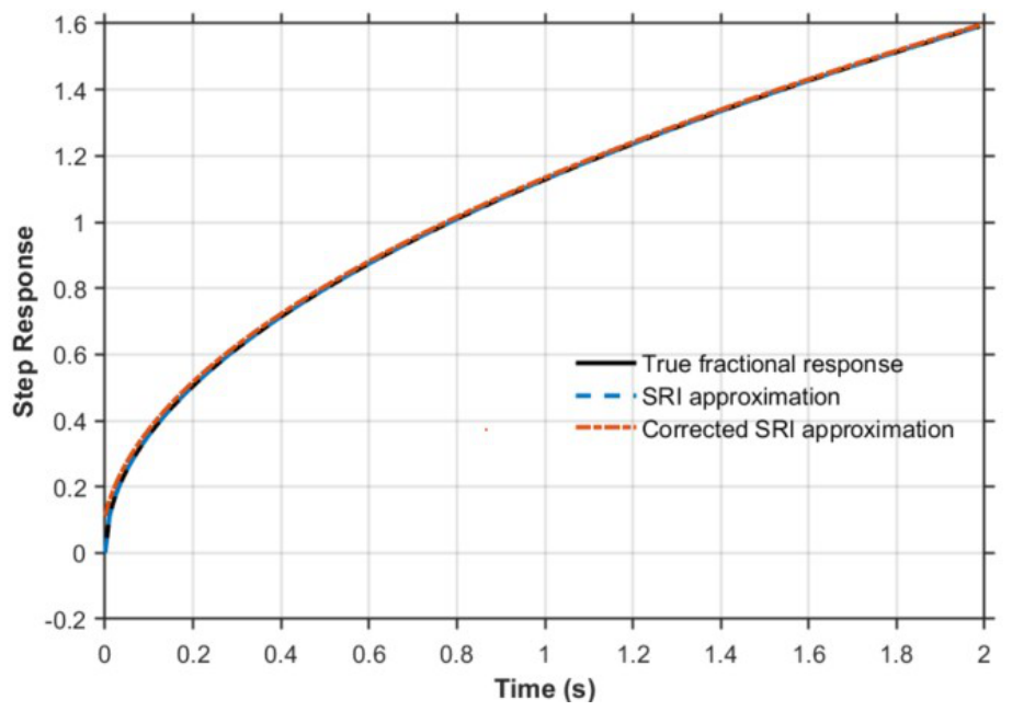
Step-Response-Invariant Approximation of .
Figure 16.
Step-Response-Invariant Approximation of .
Figure 17.
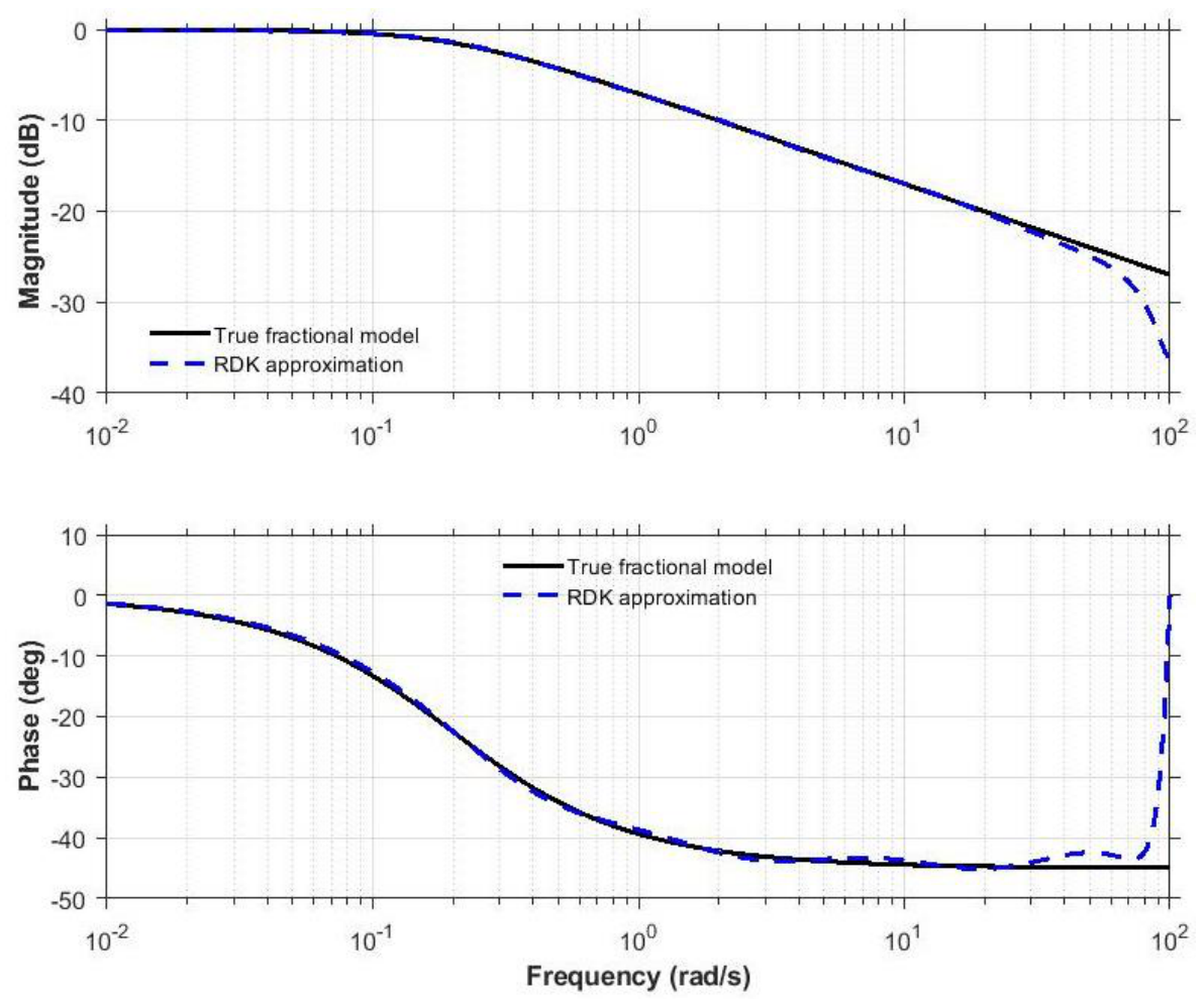
Frequency-response comparison between the original fractional-order system and the RDK discrete-time approximation.
Figure 17.
Frequency-response comparison between the original fractional-order system and the RDK discrete-time approximation.
Figure 18.
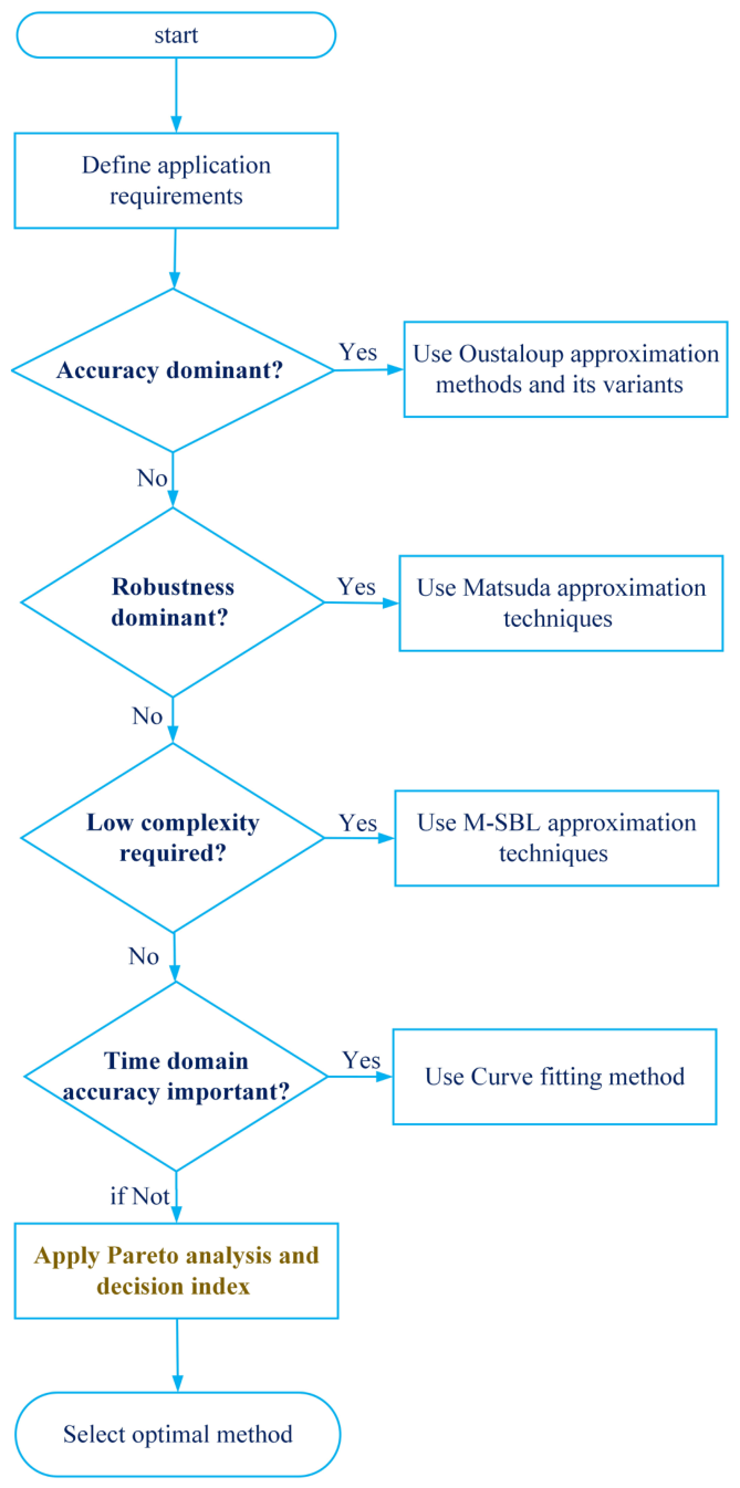
Decision framework for selecting fractional-order approximation methods based on Pareto-optimal trade-offs and application requirements.
Figure 18.
Decision framework for selecting fractional-order approximation methods based on Pareto-optimal trade-offs and application requirements.
Figure 19.
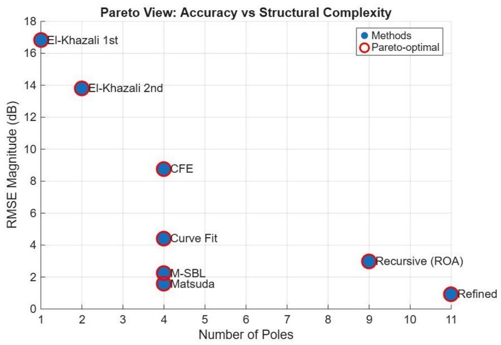
Pareto visualization showing the trade-off between approximation accuracy and structural complexity.
Figure 19.
Pareto visualization showing the trade-off between approximation accuracy and structural complexity.
Figure 20.
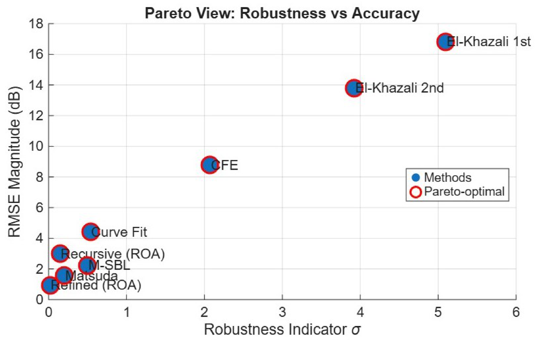
Pareto visualization showing robustness vs. approximation accuracy.
Figure 20.
Pareto visualization showing robustness vs. approximation accuracy.
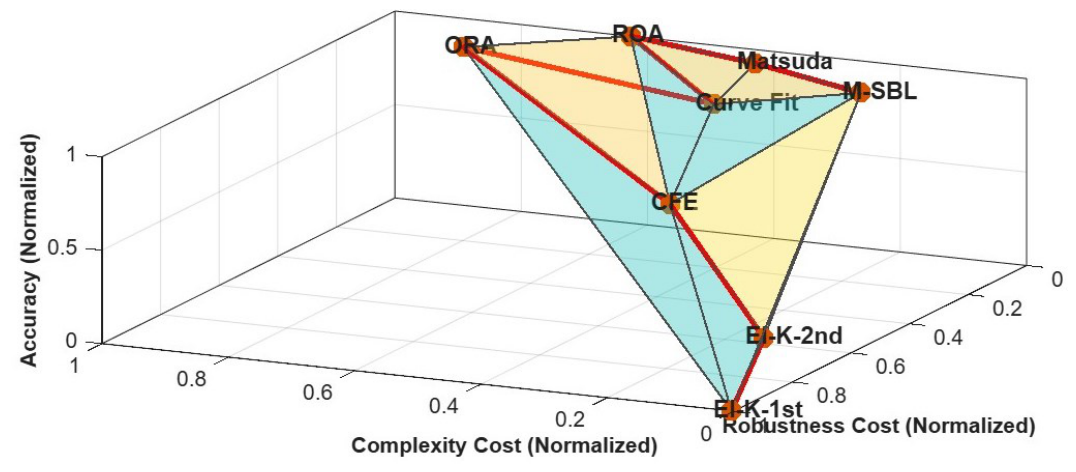
Figure 21.
Three-dimensional Pareto surface showing simultaneous optimization of complexity, robustness, and approximation accuracy.
Figure 21.
Three-dimensional Pareto surface showing simultaneous optimization of complexity, robustness, and approximation accuracy.
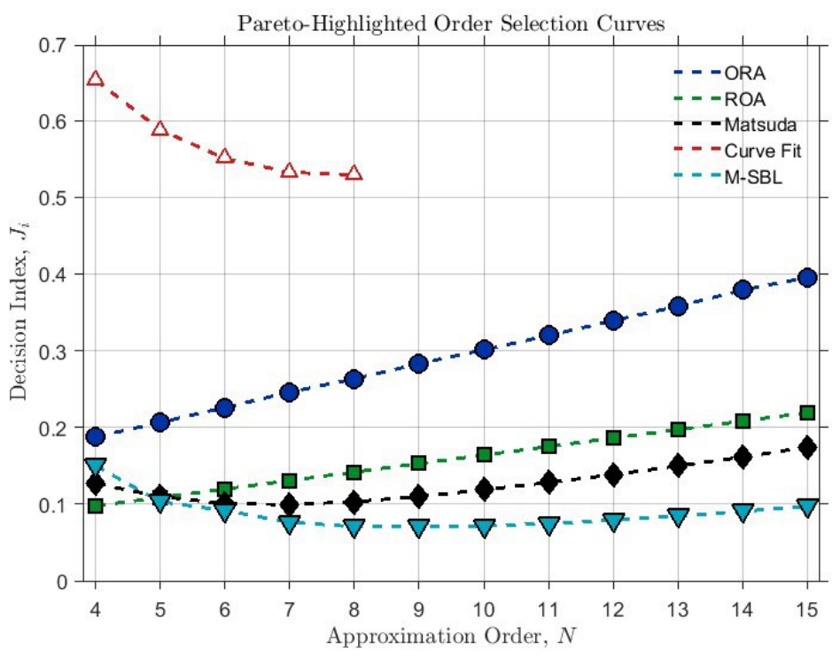
Figure 22.
Decision index vs. approximation order for fractional operator . Lower values indicate better compromise among accuracy, robustness, and complexity.
Figure 22.
Decision index vs. approximation order for fractional operator . Lower values indicate better compromise among accuracy, robustness, and complexity.
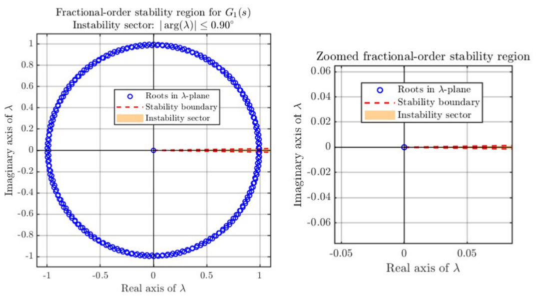
Figure 23.
Fractional-order stability region corresponding to (
121), showing that all poles lie outside the instability sector.
Figure 23.
Fractional-order stability region corresponding to (
121), showing that all poles lie outside the instability sector.
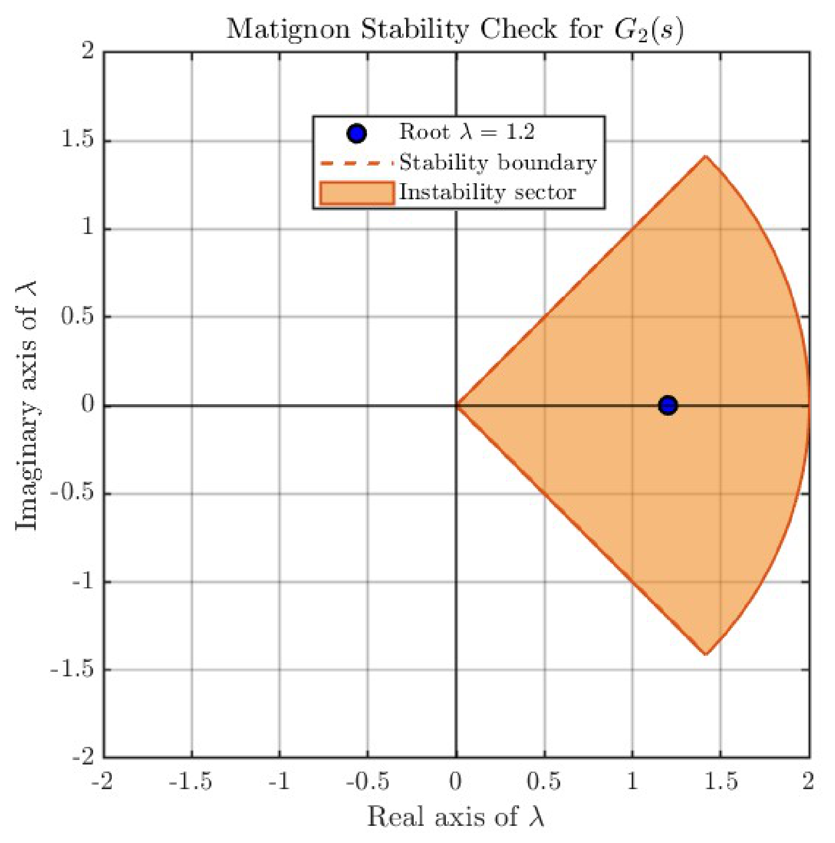
Figure 24.
Fractional-order stability region corresponding to (
124), showing that one pole lies inside the shaded region.
Figure 24.
Fractional-order stability region corresponding to (
124), showing that one pole lies inside the shaded region.
Figure 25.
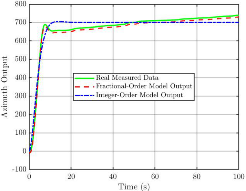
Comparison between fractional-order models identified using the refined Oustaloup approximation and the integer-order model reported in [
54].
Figure 25.
Comparison between fractional-order models identified using the refined Oustaloup approximation and the integer-order model reported in [
54].
Figure 26.
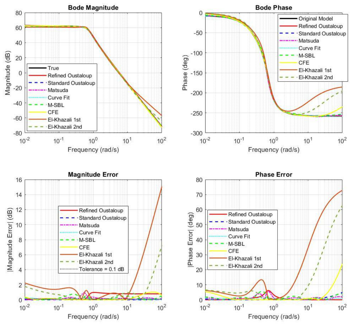
Bode plot comparison of fractional-order approximation methods for the Equation (
126) within the frequency range
rad/s.
Figure 26.
Bode plot comparison of fractional-order approximation methods for the Equation (
126) within the frequency range
rad/s.
Figure 27.
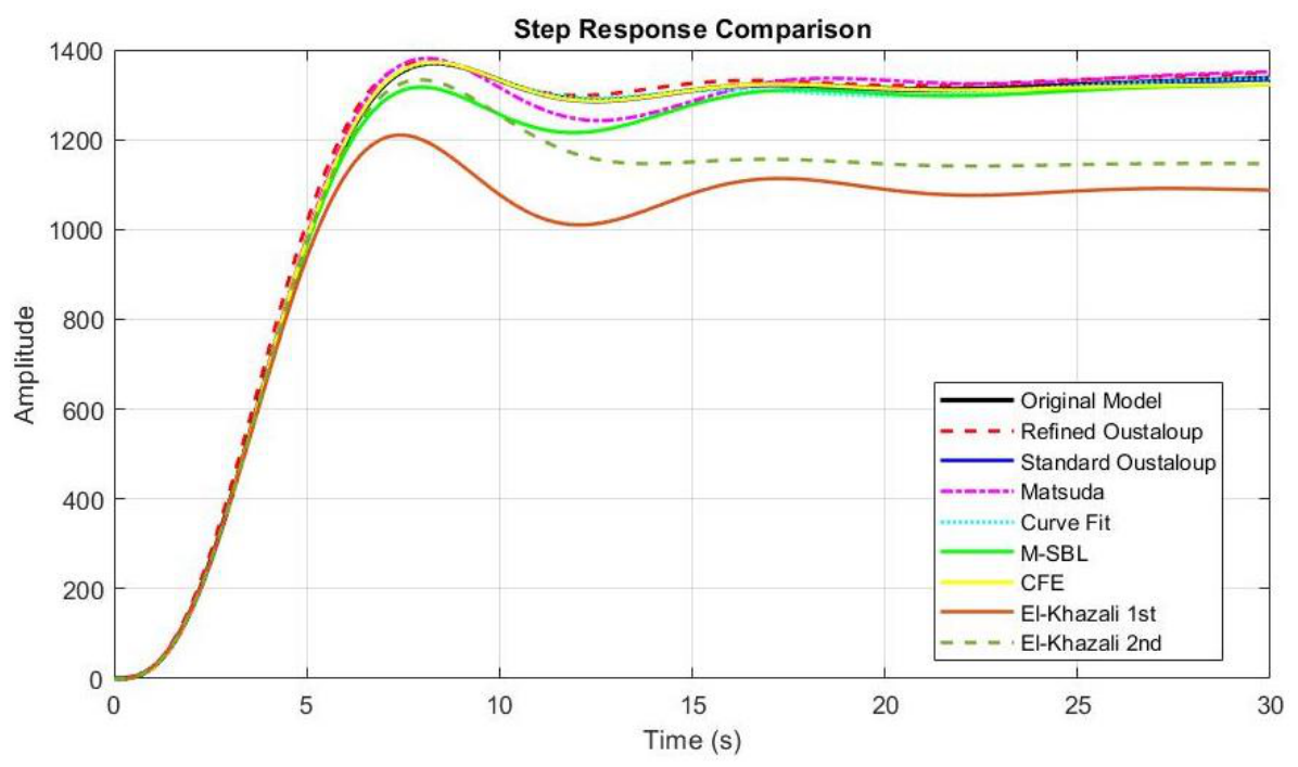
Step response comparison of fractional-order approximation methods for Equation (
126).
Figure 27.
Step response comparison of fractional-order approximation methods for Equation (
126).
Table 1.
Frequency- and time-domain performance comparison of third-, fifth-, and eighth-order ORA and ROA models of over the frequency band rad/s.
Table 1.
Frequency- and time-domain performance comparison of third-, fifth-, and eighth-order ORA and ROA models of over the frequency band rad/s.
| N | RMSEm (dB) | RMSEp (deg) | Maxm (dB) | Maxp (deg) | IAE | ISE |
|---|
| ORA | ROA | ORA | ROA | ORA | ROA | ORA | ROA | ORA | ROA | ORA | ROA |
|---|
| 3 | 7.3486 | 4.3375 | 25.939 | 21.006 | 20 | 14.439 | 44.745 | 44.109 | 0.10501 | 0.40243 | 0.63739 | 5.9320 |
| 5 | 7.3549 | 4.3374 | 25.828 | 20.996 | 20 | 14.439 | 44.727 | 44.091 | 0.09153 | 0.38693 | 0.63805 | 5.9314 |
| 8 | 7.3579 | 4.3378 | 25.789 | 20.995 | 20 | 14.439 | 44.719 | 44.083 | 0.09216 | 0.38651 | 0.63824 | 5.9314 |
Table 2.
Frequency- and time-domain performance comparison of fifth-order recursive and refined Oustaloup approximation models of over different frequency bands.
Table 2.
Frequency- and time-domain performance comparison of fifth-order recursive and refined Oustaloup approximation models of over different frequency bands.
| | RMSEm (dB) | RMSEp (deg) | Maxm (dB) | Maxp (deg) | IAE | ISE |
|---|
| ORA | ROA | ORA | ROA | ORA | ROA | ORA | ROA | ORA | ROA | ORA | ROA |
|---|
| | 7.3549 | 4.3374 | 25.828 | 20.996 | 20 | 14.439 | 44.727 | 44.091 | 0.09153 | 0.38693 | 0.63805 | 5.9314 |
| | 13.46 | 9.6351 | 32.678 | 28.962 | 30 | 24.437 | 44.972 | 44.908 | 0.39295 | 0.24305 | 0.23298 | 0.024486 |
| | 20.696 | 16.213 | 38.415 | 35.26 | 40 | 34.437 | 44.997 | 44.991 | 3.0302 | 0.47211 | 1.284 | 0.50029 |
Table 3.
Continued fraction expansion (CFE) approximations of
for different orders [
30].
Table 3.
Continued fraction expansion (CFE) approximations of
for different orders [
30].
| Order | Terms | CFE Approximation of |
|---|
| 1 | 2 | |
| 2 | 4 | |
| 3 | 6 | |
| 4 | 8 | |
| 5 | 10 | |
Table 4.
Frequency- and time-domain performance of CFE approximations of .
Table 4.
Frequency- and time-domain performance of CFE approximations of .
| Order | Approx. T.F. | RMSE | Max | Time | Freq. and BW |
|---|
| Mag. | Phase | Mag. | Phase | IAE | ISE | | | BW |
|---|
| 1 | | 15.383 | 37.978 | 30.458 | 44.98 | 2.993 | 1.367 | 0.13 | 7.8 | 7.67 |
| 2 | | 12.15 | 34.66 | 26.021 | 44.95 | 0.807 | 0.67 | 0.057 | 16 | 15.943 |
| 3 | | 10.17 | 32.406 | 23.098 | 44.908 | 0.236 | 0.46 | 0.02 | 34 | 33.78 |
| 4 | | 8.77 | 30.639 | 20.915 | 44.847 | 0.119 | 0.331 | 0.015 | 53 | 52.985 |
Table 5.
Performance metrics of Matsuda approximation for different orders of .
Table 5.
Performance metrics of Matsuda approximation for different orders of .
| Order | RMSE | Max Error | Time Domain |
|---|
| Mag (dB) | Phase (deg) | Mag (dB) | Phase (deg) | IAE | ISE |
|---|
| 3 | 8.62 | 30.61 | 20.681 | 44.84 | 0.34 | 0.01 |
| 5 | 6.43 | 27.27 | 16.98 | 44.62 | 0.01 | 0.00002 |
| 8 | 4.49 | 23.69 | 13.33 | 44.12 | 0.005 | |
Table 6.
Third- and fifth-order Matsuda approximation transfer functions of .
Table 6.
Third- and fifth-order Matsuda approximation transfer functions of .
| Order (N) | Transfer Function |
|---|
| 3 | |
| 5 | |
Table 7.
Performance metrics of Matsuda approximation for different frequency bands of with fixed order .
Table 7.
Performance metrics of Matsuda approximation for different frequency bands of with fixed order .
| Frequency (rad/s) | RMSE | Max Error | Time Domain |
|---|
| | Mag (dB) | Phase (deg) | Mag (dB) | Phase (deg) | IAE | ISE |
|---|
| 0.1 | 10 | 6.43 | 27.27 | 16.98 | 44.62 | 0.01 | |
| 0.01 | 100 | 3.58 | 21.93 | 11.39 | 43.71 | 0.15 | 0.001 |
| 0.001 | 1000 | 1.10 | 13.37 | 4.03 | 38.46 | 0.97 | 0.06 |
Table 8.
Magnitude error analysis of the Charef composite approximation for different error tolerances.
Table 8.
Magnitude error analysis of the Charef composite approximation for different error tolerances.
| (dB) | | | N | RMSEm (dB) | Maxm (dB) |
|---|
| 1 | 7 | 5 | 11 | 0.0603 | 0.2797 |
| 2 | 4 | 3 | 6 | 0.1388 | 0.3005 |
| 3 | 3 | 2 | 4 | 0.6104 | 1.2754 |
Table 9.
Numerical conditioning and computational cost of the M-SBL approximation for .
Table 9.
Numerical conditioning and computational cost of the M-SBL approximation for .
| Order N | | Time (s) | RMSEm | RMSEp |
|---|
| 2 | | 0.0049 | 6.0757 | 26.024 |
| 3 | | 0.0005 | 3.8522 | 19.094 |
| 4 | | 0.0021 | 2.2259 | 14.683 |
| 5 | | 0.0016 | 1.4770 | 12.807 |
| 6 | | 0.0015 | 1.0494 | 11.660 |
| 7 | | 0.0017 | 0.7724 | 10.698 |
| 8 | | 0.0018 | 0.5791 | 9.7819 |
| 9 | | 0.0017 | 0.4431 | 8.8890 |
| 10 | | 0.0015 | 0.3540 | 8.0238 |
| 11 | | 0.0012 | 0.3054 | 7.1947 |
| 12 | | 0.0017 | 0.2882 | 6.4084 |
Table 10.
Transfer Functions of M-SBL and Curve-Fitting Approximations for at Different Orders.
Table 10.
Transfer Functions of M-SBL and Curve-Fitting Approximations for at Different Orders.
| N | M-SBL Transfer Function | Curve-Fitting Transfer Function |
|---|
| 4 | | |
| 5 | | |
| 6 | | |
Table 11.
Effect of selected frequency points on approximation performance for Matsuda, curve-fitting, and M-SBL methods.
Table 11.
Effect of selected frequency points on approximation performance for Matsuda, curve-fitting, and M-SBL methods.
| Order | Matsuda | Curve Fit | M-SBL |
|---|
| Points | RMSEm | Time (s) | Points | RMSEm | Time (s) | Points | RMSEm | Time (s) |
|---|
| 1 | 3 | 2.6947 | 0.0077 | 3 | 3.3368 | 0.0048 | 1 | 4.8390 | 0.0015 |
| 2 | 5 | 0.7246 | 0.0098 | 5 | 1.3955 | 0.0033 | 2 | 1.1554 | 0.0014 |
| 3 | 7 | 0.1956 | 0.0147 | 7 | 0.6514 | 0.0033 | 3 | 0.2320 | 0.0014 |
| 4 | 9 | 0.0853 | 0.0216 | 9 | 0.2598 | 0.0048 | 4 | 0.0400 | 0.0009 |
| 5 | 11 | 0.0226 | 0.0498 | 11 | 0.0822 | 0.0103 | 5 | 0.0109 | 0.0033 |
| 6 | 13 | 0.0084 | 0.0767 | 13 | 0.0213 | 0.0145 | 6 | 0.0048 | 0.0013 |
| 7 | 15 | 0.0036 | 0.0347 | 15 | 0.0109 | 0.0055 | 7 | 0.0017 | 0.0008 |
| 8 | 17 | 0.0009 | 0.0365 | 17 | 0.0089 | 0.0092 | 8 | 0.0004 | 0.0009 |
Table 12.
Transfer Functions of Equal-Ripple and Exact-Phase Approximations for at Different Stages.
Table 12.
Transfer Functions of Equal-Ripple and Exact-Phase Approximations for at Different Stages.
| N | Equal-Ripple Transfer Function | Exact-Phase Transfer Function |
|---|
| 1 | | |
| 2 | | |
| 3 | | |
Table 13.
Performance comparison of approximation methods for , including accuracy, robustness, computational complexity, and stability.
Table 13.
Performance comparison of approximation methods for , including accuracy, robustness, computational complexity, and stability.
| Method | Stable | Poles | Zeros | | | RMSEm | RMSEp | Maxm | Maxp | IAE | ISE | | | | Pareto |
|---|
| ORA | Yes | 9 | 9 | −0.003 | 0.0254 | 2.98 | 18.78 | 10.02 | 42.34 | 0.14 | 0.95 | 0.10 | 0.15 | 0.31 | Yes |
| ROA | Yes | 11 | 11 | −0.00045 | 0.0031 | 0.93 | 11.06 | 4.17 | 35.86 | 0.53 | 10.32 | 0.45 | 0.02 | 0.27 | Yes |
| Matsuda | Yes | 4 | 4 | −0.01 | 0.0154 | 1.57 | 16.09 | 5.28 | 40.50 | 0.81 | 6.82 | 0.89 | 0.20 | 0.22 | Yes |
| Curve-Fit | Yes | 4 | 4 | −0.12 | 0.0175 | 4.41 | 22.36 | 16.15 | 44.66 | 0.82 | 4.81 | 0.97 | 0.54 | 0.29 | Yes |
| M-SBL | Yes | 4 | 4 | −0.01 | 0.0038 | 2.23 | 14.71 | 5.97 | 38.45 | 1.16 | 5.47 | 1.52 | 0.50 | 0.17 | Yes |
| CFE | Yes | 4 | 4 | −0.13 | 0.0133 | 8.77 | 30.64 | 20.92 | 44.85 | 0.21 | 0.46 | 1.51 | 2.07 | 0.36 | Yes |
| El-Khazali-1st | Yes | 1 | 1 | −2.41 | 0.0017 | 16.82 | 38.81 | 32.34 | 44.99 | 7.36 | 3.24 | 5.95 | 5.10 | 0.66 | Yes |
| El-Khazali-2nd | Yes | 2 | 2 | −0.62 | 0.0015 | 13.81 | 36.12 | 28.34 | 44.97 | 3.20 | 1.43 | 4.06 | 3.92 | 0.49 | Yes |
Table 14.
Optimal approximation order selected using the Pareto-based decision index for .
Table 14.
Optimal approximation order selected using the Pareto-based decision index for .
| Method | Optimal N | Min. |
|---|
| ORA | 4 | 0.1876 |
| ROA | 4 | 0.0976 |
| Matsuda | 7 | 0.0998 |
| Curve Fit | 8 | 0.5285 |
| M-SBL | 9 | 0.0704 |
Table 15.
Comprehensive performance comparison of approximation methods for the Equation (
126) at order 5, including accuracy, robustness, and decision index
.
Table 15.
Comprehensive performance comparison of approximation methods for the Equation (
126) at order 5, including accuracy, robustness, and decision index
.
| Method | Stable | Poles | | RMSEm | RMSEp | Maxm | Maxm | IAE | ISE | |
|---|
| Refined Oustaloup | No | 36 | 0.001 | 0.61 | 1.61 | 0.98 | 6.22 | 382.54 | 7771.50 | 0.35 |
| Standard Oustaloup | Yes | 32 | −0.003 | 0.01 | 1.15 | 0.04 | 4.90 | 57.44 | 136.21 | 0.28 |
| Matsuda | Yes | 16 | −0.0001 | 0.24 | 1.66 | 0.94 | 5.66 | 437.31 | 10,232.00 | 0.23 |
| Curve Fit | Yes | 16 | −0.01 | 0.12 | 0.74 | 0.30 | 2.20 | 137.32 | 1510.40 | 0.21 |
| M-SBL | Yes | 16 | −0.0006 | 0.31 | 1.99 | 0.75 | 5.71 | 749.38 | 35,860.00 | 0.25 |
| CFE | Yes | 14 | −0.07 | 0.38 | 5.00 | 1.04 | 23.89 | 81.04 | 563.92 | 0.20 |
| El-Khazali 1st | Yes | 5 | −0.18 | 4.29 | 31.19 | 15.07 | 72.79 | 5525.70 | 1.27 | 0.74 |
| El-Khazali 2nd | Yes | 8 | −0.24 | 1.64 | 20.45 | 7.26 | 62.65 | 3400.00 | 5.44
| 0.47 |




 ,
,