Relationship of Multifractal and Entropic Properties of Global Seismic Noise with Major Earthquakes, 1997–2025

Abstract

A method for analyzing long-term (1997–2025) continuous records of low-frequency global seismic noise measured at a network of 229 broadband seismic stations distributed across the Earth’s surface is proposed in this study. The method is based on the use of nonlinear multifractal and entropy statistics, evaluated daily in successive time intervals, of first-principal component analysis, correlation analysis, and parametric models of point process intensity. The relationships between changes in seismic noise properties and the response of noise properties to the irregularity of the Earth’s rotation with the sequence of strong earthquakes, including those of a predictive nature, are investigated.

1. Introduction

Tectonic processes in the lithosphere preceding strong earthquakes are reflected in changes in the properties of seismic noise [1,2,3]. The passage of atmospheric cyclones and the impact of ocean waves on the coast and shelf are the main sources of low-frequency seismic noise [4,5,6,7,8,9,10]. Studying the characteristics of seismic noise allows us to obtain information about the structure of the Earth’s crust [11].

This paper examines continuous seismic noise records from early 1997 to late 2025, recorded at a network of 229 broadband seismic stations located worldwide. The following properties of noise waveforms are analyzed: the entropy of the wavelet coefficient distribution, the Donoho–Johnstone (DJ) index (the fraction of wavelet coefficients with large absolute values), and the singularity spectrum support width. These statistics are indicators of seismic noise complexity and are calculated daily at each station. An auxiliary network of 50 reference points is considered. For each reference point, the median values of noise properties are found from the five nearest stations that are operational on the current day. The use of reference points allows for a continuous time series of noise property changes with a time step of 1 day and overcomes methodological difficulties associated with recording gaps at stations. Further analysis is based on the principal component analysis (PCA) method, calculated for the noise properties used both at each reference point and across all reference points. The principal components are estimated over a 365-day sliding time window. The relationship between seismic noise properties and the sequence of strong earthquakes (magnitude of at least 7) is analyzed using a parametric model of interacting point processes. In this model, one process is the sequence of seismic events, and the other is the sequence of local extremes of seismic noise properties.

The article continues the studies carried out in [12,13] to investigate the correlation and coherence properties of low-frequency seismic noise on a global scale covering the entire planet.

2. Data

The vertical components of continuous seismic noise records with 1 s sampling intervals are analyzed. Data were downloaded from the Incorporated Research Institutions for Seismology (IRIS) website [14] from 229 broadband seismic stations of three networks:

Global Seismographic Network: http://www.iris.edu/mda/_GSN (accessed on 4 February 2026)

GGEOSCOPE: http://www.iris.edu/mda/G (accessed on 4 February 2026)

GEOFON: http://www.iris.edu/mda/GE (accessed on 4 February 2026)

The data were downloaded using a Python Toolbox “ObsPy”, version 1.3.1, for seismological observatories [15]. Seismic noise records with a sampling rate of 1 Hz (LHZ records) were considered for 29 years of registration (from 1 January 1997 to 31 December 2025). These data were converted to 1 min time series by calculating averages for successive 60 s time intervals.

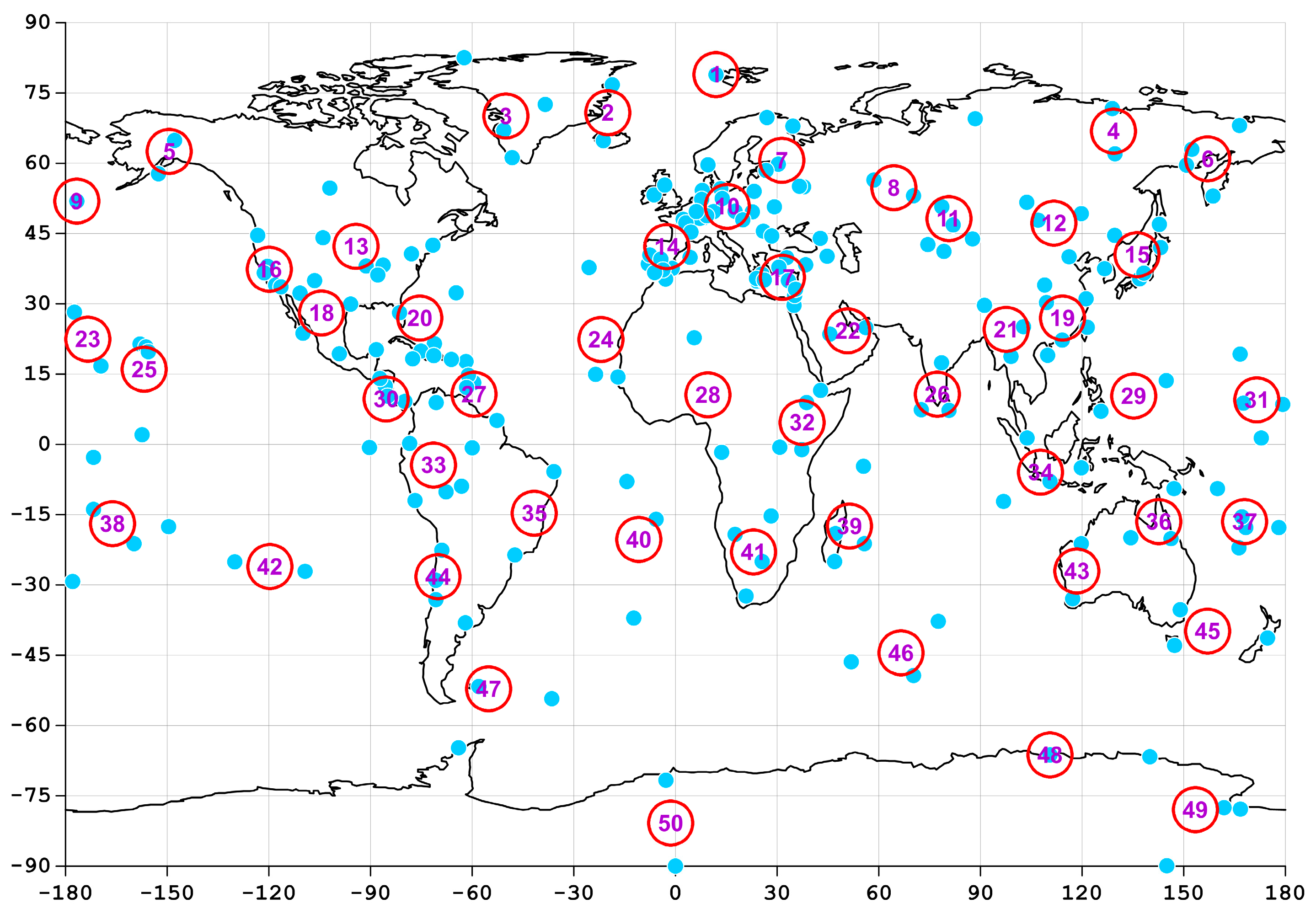
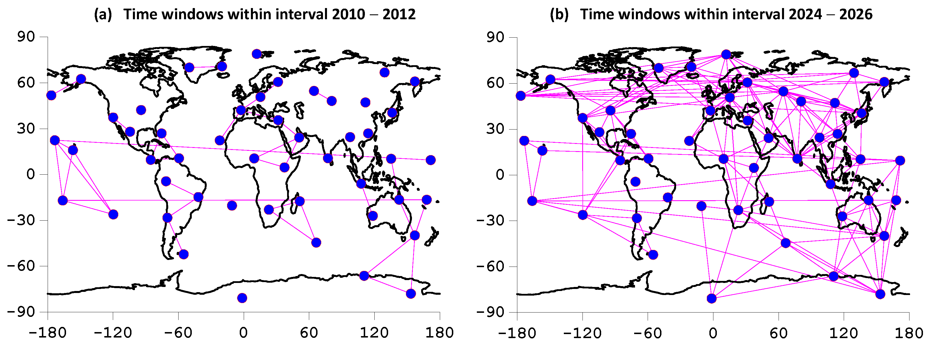
Consider an auxiliary network of 50 reference points, which are determined using a hierarchical cluster analysis of the positions of 229 seismic stations using the “far neighbor” method [12]. The location of 229 seismic stations and 50 reference points is shown in Figure 1. The numbering of reference points is carried out as the latitude of the point decreases.

3. Properties of Seismic Noise

The minimum entropy of a time series is determined by the formula $En=-{\displaystyle \sum _k{q}_k\cdot \ln (}{q}_k)/\ln (N)$, where $q_k=w_k^2/{\displaystyle {\sum }_j{w}_j^2}$, $w_k$ are the wavelet coefficients of the signal decomposition, and $N$ is the total number of coefficients $w_k$. Seventeen orthogonal Daubechies wavelets were used: 10 ordinary minimum support bases with vanishing moments from 1 to 10 and seven so-called Daubechies symlets [16] with vanishing moments from 4 to 10. In each time window, the wavelet for which the value $En$ is minimal is selected. These orthogonal wavelets have the smallest support length for a given smoothness—the number of vanishing moments.

The Donoho–Johnstone (DJ) wavelet-based index $\gamma$ is the ratio of “large” wavelet coefficients in absolute value to their total number. By definition $0\le \gamma \le 1$, the threshold separating “large” wavelet coefficients is $\mathsf{\sigma }\sqrt{2\cdot \ln N}$, where $\mathsf{\sigma }=med\left\{\left|w_k^{(1)}\right|,k=1,\dots ,N/2\right\}/0.6745$ is a robust estimate of the standard deviation of the normal distribution, $w_k^{(1)}$ are the wavelet coefficients at the first detail level of decomposition, and $N/2$ is the number of such coefficients [16,17].

The singularity spectrum support width $\Delta \alpha$ is considered a measure of the diversity of the stochastic behavior of the signal $u(t)$. It is defined as $\Delta \alpha ={\alpha }_{\max }-{\alpha }_{\min }$, where ${\alpha }_{\min }$ and ${\alpha }_{\max }$ are the minimum and maximum values of the Hölder–Lipschitz exponent [18], which governs the behavior of the signal in the vicinity of the time instant $t$: $|u(t+\frac{\delta }{2})-u(t-\frac{\delta }{2})|\sim |\delta {|}^{\alpha }, \delta \to 0$. For a monofractal signal, the exponent $\alpha$ is the same for all time instants $t$. If this exponent differs, then the signal is multifractal [19].

After switching to a 1 min sampling time step, the seismic records from each station were divided into 1-day-long time fragments (1440 samples), and the parameters $(\gamma ,\Delta \alpha ,En)$ of daily seismic noise signals were calculated for each fragment. The multifractal DFA method [20] was used to calculate the values of the singularity spectrum support width. The methods for estimating the parameters $\gamma$, $\Delta \alpha$ and $En$ for seismic noise records in a sliding time window are described in detail in [21,22]. Thus, time series of values with a 1-day time step were obtained for each of the seismic stations.

The entropy value $En$ used in this paper, defined through the coefficients of the orthogonal wavelet decomposition, has features in common with multiscale entropy used, for example, in biology [23,24]. In [25,26], entropy is used within the framework of the natural time approach for seismic data analysis. In [27], non-extensive Tsallis entropy is used for processing seismic noise data.

The use of multifractal analysis to study the behavior of various complex systems has a long history. Particular attention is paid to the effect of parameter $\Delta \alpha$ reduction (loss of multifractality) preceding changes in system properties. In medicine, a decrease in the $\Delta \alpha$ value of various parameters accompanies age-related changes [28,29,30]. In [31,32], multifractal analysis is used to analyze geoelectric signals and wind speed. Within the framework of the natural time approach, multifractal analysis is used to study both seismicity and other time sequences [33].

Let us denote by ${\tilde{\mathsf{\gamma }}}_j(t)$, $\Delta {\tilde{\mathsf{\alpha }}}_j(t)$, $\tilde{E}{n}_j(t)$, $j=1,\mathrm{...50}$, the daily time series of parameters at 50 reference points of the seismic noise observation network, which are calculated as the medians of the values at the five nearest operational (without data gaps for this day) seismic stations.

4. First Principal Component and Weighted Mean of Multiple Time Series

In the future, we will need to calculate the first principal components and weighted averaging of multivariate time series. The values of the parameters $(\gamma ,\Delta \alpha ,En)$ introduced above are calculated in successive time windows of a certain length, resulting in a 3-dimensional time series, the properties of which are further studied jointly. The used properties of seismic noise reflect the change in its structure; in particular, we are interested in the phenomenon of noise structure simplification as a sign that precedes strong earthquakes. Attempts to determine the “best” property of noise led to the idea of using the principal component approach [34,35,36] to aggregate time series $(\gamma ,\Delta \alpha ,En)$ into one scalar time series. Since the purpose of the analysis is to study the variability of noise properties both in time and space, the principal component method was applied in a sliding time window.

Let us consider a multiple time series $p(t)={(p_1(t),\dots ,p_m(t))}^T$, $t=0,1,\dots$ of the dimensionality $m$. It is necessary to estimate two types of its first principal component in the moving time window of the length $L$ samples. For this purpose, let us consider samples with time indices $t$ under the condition $s-L+1\le t\le s$, where $s$ is the right-most end of the moving time window. Let us perform normalization of multiple time series components within the current time window:

$$q_k^{(s)}(t)=(p_k(t)-{\overline{p}}_k^{(s)}),\hspace{1em}{\overline{p}}_k^{(s)}={\displaystyle \sum _{t=s-L+1}^s{p}_k(t)/L},\hspace{1em}k=1,\dots ,m$$

(1)

$$r_k^{(s)}(t)=q_k^{(s)}(t)/{\sigma }_k^{(s)},\hspace{1em}{\left({\sigma }_k^{(s)}\right)}^2={\displaystyle \sum _{t=s-L+1}^s(q_k^{(s)}(t)}{)}^2/(L-1),\hspace{1em}k=1,\dots ,m$$

(2)

Let us consider two correlation matrices $Q(s)$ and $R(s)$ of the size $m\times m$, which are calculated by the formulae:

$$Q(s)=\left(Q_{kj}^{(s)}\right),\hspace{1em}{Q}_{kj}^{(s)}={\displaystyle \sum _{t=s-L+1}^s{q}_k^{(s)}(t)q_j^{(s)}(t)/L,\hspace{1em}k,j=1,\dots ,m}$$

(3)

$$R(s)=\left(R_{kj}^{(s)}\right),\hspace{1em}{R}_{kj}^{(s)}={\displaystyle \sum _{t=s-L+1}^s{r}_k^{(s)}(t)r_j^{(s)}(t)/L,\hspace{1em}k,j=1,\dots ,m}$$

(4)

Let ${\varphi }^{(s)}={({\varphi }_1^{(s)},\dots ,{\varphi }_m^{(s)})}^T$ and ${\phi }^{(s)}={({\phi }_1^{(s)},\dots ,{\phi }_m^{(s)})}^T$ be eigenvectors of the matrices $Q(s)$ and $R(s)$ corresponding to their maximum eigenvalues. Let us define the first principal component $P^{(s)}(t)$ and the weighted mean $W^{(s)}(t)$ of multiple time series $p(t)$ within the current time window by the formulae:

$$P^{(s)}(t)={\displaystyle \sum _{k=1}^m{\varphi }_k^{(s)}\cdot r_k^{(s)}(t)},\hspace{1em}{W}^{(s)}(t)={\displaystyle \sum _{k=1}^m{({\phi }_k^{(s)})}^2\cdot q_k^{(s)}(t)}$$

(5)

and define the scalar time series $P(t)$ and $W(t)$ of the adaptive first principal component and the weighted mean in the moving time window by the formulae:

$$P(t)=\left\{\begin{array}{c}{P}^{(L-1)}(t), 0\le t\le (L-1)\hfill \\ P^{(t)}(t), t\ge L\hspace{1em}\hspace{1em}\hspace{1em}\hspace{1em}\hfill \end{array}\right.,\hspace{1em}W(t)=\left\{\begin{array}{c}{W}^{(L-1)}(t), 0\le t\le (L-1)\hfill \\ W^{(t)}(t), t\ge L\hspace{1em}\hspace{1em}\hspace{1em}\hspace{1em}\hfill \end{array}\right.$$

(6)

Equations (1)–(6) are applied independently within each time window. According to these formulae, within the first time window time series, $P(t)$ and $W(t)$ consist of $L$ values corresponding to (3–5). In all subsequent windows, $P(t)$ and $W(t)$ correspond to the only sample in the right-most time index. Thus, outside the first time window, $P(t)$ and $W(t)$ are dependent on the past values of $p(t)$.

The standard first component $P(t)$ is used when it is necessary to aggregate heterogeneous components of a multidimensional time series, for example, a daily time series of seismic noise properties $(\gamma ,\Delta \alpha ,En)$ at a single reference point. In this case, the time series dimension is $m=3$. Weighted averaging $W(t)$ of time series components is used when the time series components are homogeneous, for example, to average the time series of principal components at all reference points. In this case, the time series dimension is $m=50$. In the following, we will agree to call these two variants of using the principal component method P-averaging and W-averaging.

A moving time window with a period of 365 days will be used. The choice of this period is quite natural because of the presence of annual periodicity in almost all background processes in the Earth’s crust. We assume that the period of the sliding time window of 365 days ensures relative stationarity of the behavior of low-frequency seismic noise within this time window.

At each reference point with a number $j$, we calculate the first principal component of three time series ${\tilde{\mathsf{\gamma }}}_j(t)$, $\Delta {\tilde{\mathsf{\alpha }}}_j(t)$, $\tilde{E}{n}_j(t)$ using the P-averaging method (1–6) in a sliding time window of 365 days in length and denote it as $P_{\mathsf{\gamma },\Delta \mathsf{\alpha },En}^{(j)}(t)$. It should be noticed that the values of seismic noise parameters and their first principal component are dimensionless. 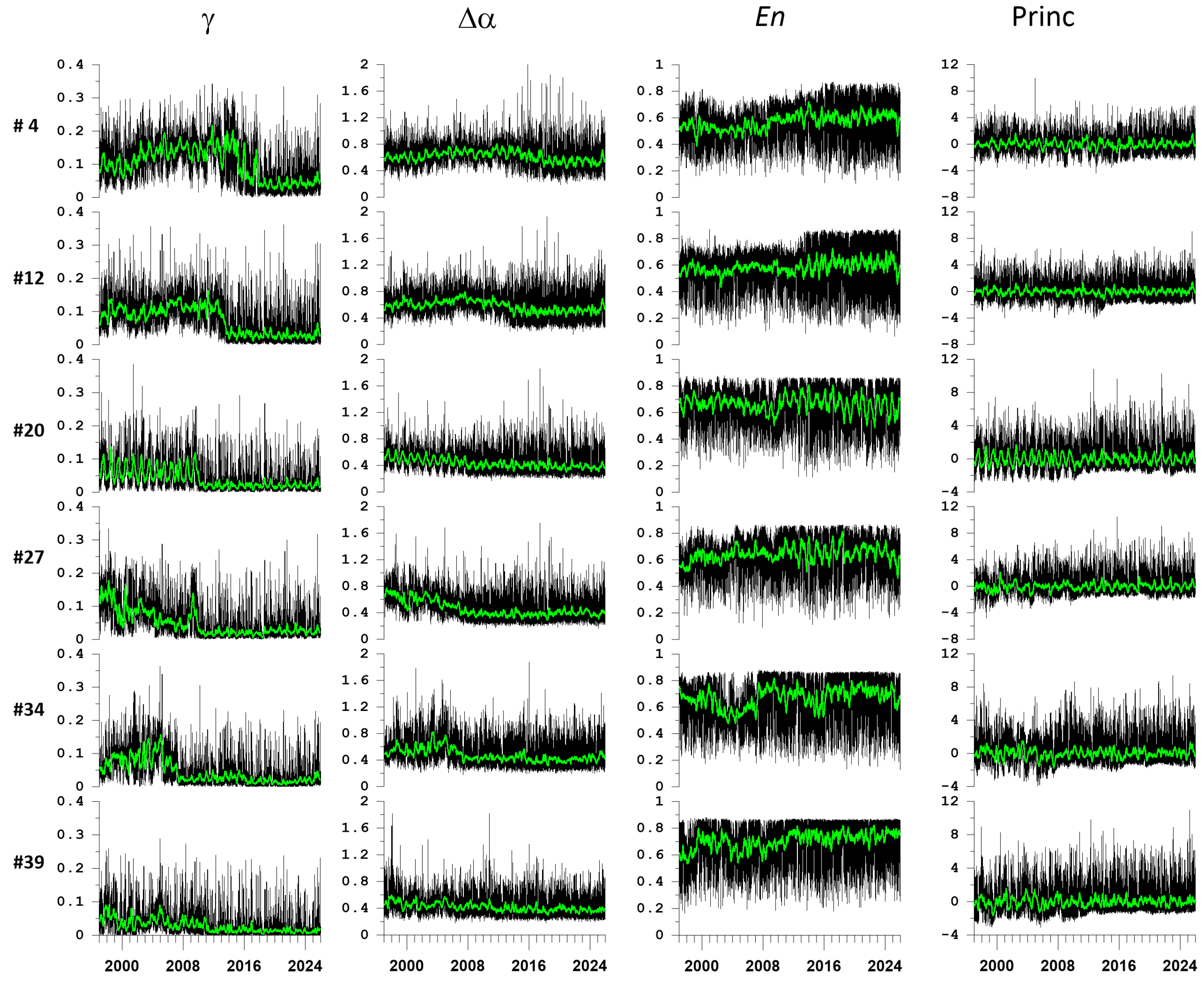Figure 2 shows graphs of the time series of seismic noise properties and their first principal components, calculated in a sliding adaptation time window of 365 days for six reference points.

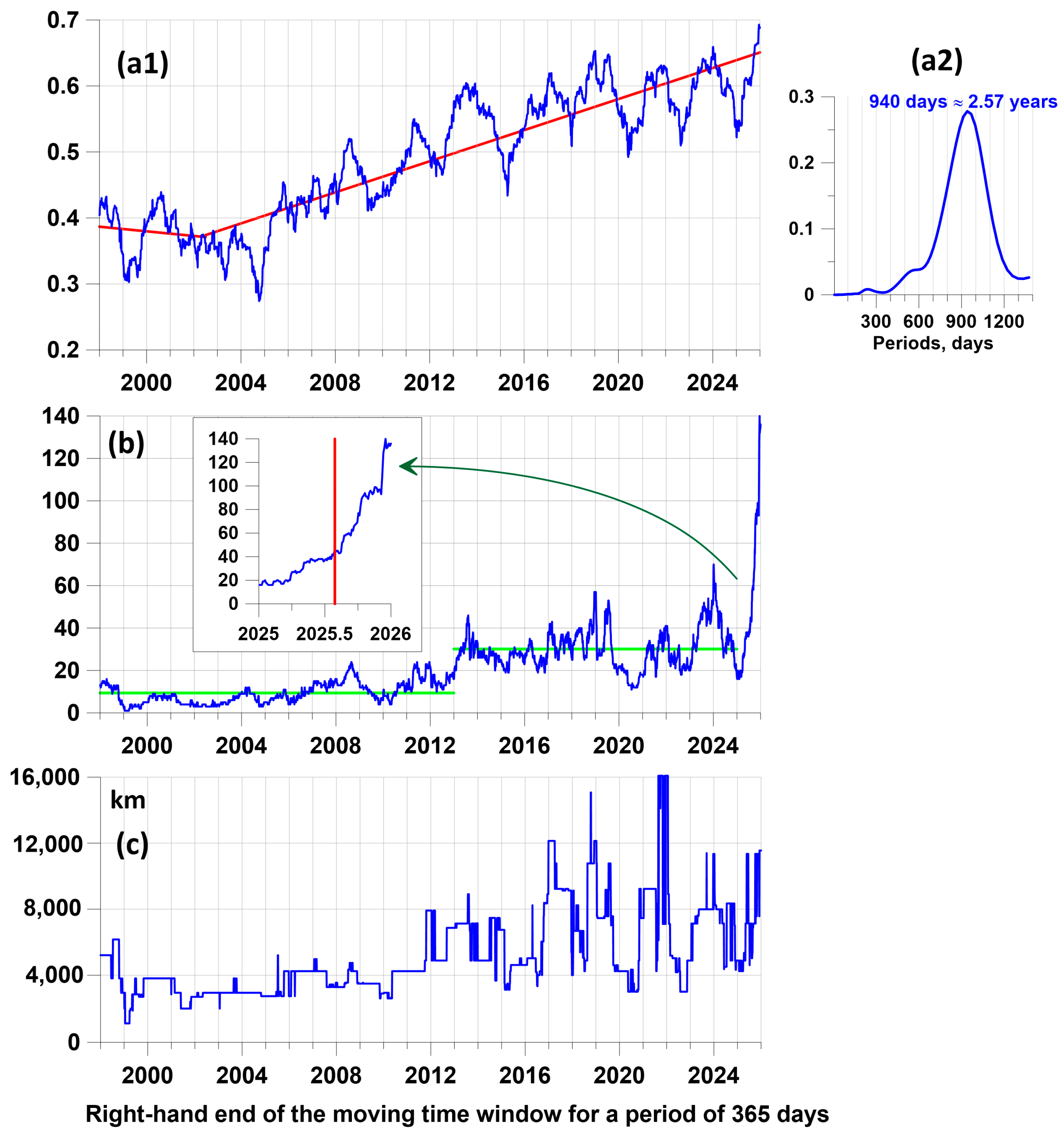
Let us estimate the temporal variability of strong correlations between the first principal components of seismic noise properties at different reference points. To do this, we calculate the average absolute correlations of the principal components $P_{\mathsf{\gamma },\Delta \mathsf{\alpha },En}^{(j)}(t)$ between all reference points over a 365-day sliding time window. Figure 3(a1) shows a graph of these average correlations, which shows a trend of increasing spatial correlations since 2002.5 (end of June 2002). It is easy to see near-periodic oscillations in this graph. To accurately estimate the period of these oscillations, we calculate the mean squared wavelet coefficients of the continuous Morlet wavelet transform for the curve in Figure 3(a1), starting with the 2004 time stamp. The Morlet transform of the signal $y(s)$ is defined by a formula [16]:

$$c(t,\eta )={\displaystyle \frac{1}{\sqrt{\eta }}}{\displaystyle \underset{-\infty }{\overset{+\infty }{\int }}y(s)\cdot \psi }\left({\displaystyle \frac{s-t}{\eta }}\right)ds,\hspace{1em}\eta >0,\hspace{1em}\psi (t)={\displaystyle \frac{1}{{\pi }^{1/4}}}\exp (-t^2/2-i\pi t)$$

(7)

The Morlet spectrum is defined as the mean value of $|c(t,\eta ){|}^2$ with respect to time moments $t$ for a set of periods $\eta$ of oscillations. This spectrum is shown in Figure 3(a2), in which the maximum oscillation energy is reached at a period of 940 days, which corresponds to 2.57 years.

We set a threshold of 0.8 for correlations and calculated the change in the number of reference point pairs for which the correlation exceeds this threshold. This dependence is shown in Figure 3b, which shows that the number of strong spatial correlations increased essentially after 2013.

The time point 2013, corresponding to the right-hand end of the time window, was found using the method of variance analysis [35] by comparing the mean values in two time intervals between the trial time point, separating these intervals for the fragment 1998–2025. The final fragment of the positions of the right-hand end of the time window 2025–2026 stands out, especially due to a remarkable anomaly in the behavior of the number of pairs of reference points with strong correlations: in the second half of 2025, the number of strong correlations tripled in six months. We suggest that this effect may be related to the mega-earthquake in Kamchatka on 29 July 2025, with a magnitude of 8.8 [37,38]. Figure 3c shows the dependence of the maximum distances between reference points for which a strong correlation greater than 0.8 emerged on the right-hand end position of a 365-day sliding time window. This dependence also reveals a step in the distances of strong spatial correlations after 2012.

In Figure 4, strong correlations between the data points are visualized as two connectivity diagrams for time windows spanning two 2-year time intervals. Figure 4b corresponds to the time window with the largest number of strong correlations.

5. Probability Densities of Extreme Values

In what follows, we distinguish two cases that consider the extreme values of the seismic noise statistics. We agree to denote the first case by $({\gamma }_{\min },\Delta {\alpha }_{\min },E{n}_{\max })$, in which we analyze the joint spatial distribution or local extrema in the time realizations of the minimum values of the index $\gamma$ and $\Delta \alpha$ and the maximum values of entropy $En$. We denote the second case by $({\gamma }_{\max },\Delta {\alpha }_{\max },E{n}_{\min })$, for which we consider the joint spatial distribution or local extrema in the time realizations of the maximum values of index $\gamma$ and $\Delta \alpha$ and the minimum values of entropy $En$. These two cases are antagonistic. Case 1 corresponds to a simplification of the seismic noise structure and its properties approaching white noise. The opposite, case 2, corresponds to enrichment of the noise structure and, as a rule, corresponds to the appearance of chaotic high-amplitude spikes in noise realizations.

Let us study the variability in the spatial distribution of extreme values of seismic noise properties. For this purpose, we consider a regular grid of 100 nodes by longitudes and 50 nodes by latitudes, covering all area of the Earth. Let $U$ be any value of $\gamma$, $\Delta \alpha$ or $En$. For each grid node $(i,j)$ and for each day with number $t$, we find the five nearest working seismic stations, which provide five values of $U$. Let us denote $U_{ij}^{(t)}$ as the median value of these five properties at node $(i,j)$ on a day with number $t$. For each daily set of $U_{ij}^{(t)}$ values with a discrete time index $t$, we find the coordinates of the nodes ${\zeta }_{mn}^{(t)}=(Lo{n}_m^{(t)},La{t}_n^{(t)})$ at which extreme values of $U$ are reached relative to all other nodes of the regular grid for the two cases introduced above, $({\gamma }_{\min },\Delta {\alpha }_{\min },E{n}_{\max })$ and $({\gamma }_{\max },\Delta {\alpha }_{\max },E{n}_{\min })$. The two-dimensional probability distribution function of the vectors ${\zeta }_{mn}^{(t)}$ is calculated within the time interval $t\in [t_0,t_1]$ for each node ${\zeta }_{ij}$ of the regular grid using the Parzen–Rosenblatt estimate with the Gaussian kernel function [36]:

$$p({\zeta }_{ij}|t_0,t_1)={\displaystyle \frac{1}{2\pi D^2(h)M_{t_0,t_1}}}{\displaystyle \sum _{t=t_0}^{t_1}{\displaystyle \sum _{mn}\exp \left(-\frac{{\rho }^2({\zeta }_{ij},{\zeta }_{mn}^{(t)})}{2D^2(h)}\right)}}$$

(8)

Here $h$ is the kernel averaging radius in spherical degrees; $t_0,t_1$ are integer indices that number the daily maps; and $M_{t_0,t_1}=(t_1-t_0+1)$ is the number of daily maps in the time interval under consideration. ${\rho }^2(\xi ,\zeta )$ is a squared spherical distance between points $\xi$ and $\zeta$ at the Earth’s surface; $D^2(h)$ is the square of the spherical distance between points on the Earth’s surface, corresponding to the value $h$. A smoothing bandwidth of $h={15}^{\circ }$ was used. This value corresponds to a distance of ≈1700 km along the Earth’s surface and is defined as the maximum of the histogram of the distribution of distances between all pairs of the nearest reference points [12].

Let us calculate the 2-dimensional distribution densities (8) of extreme values in successive time windows of 10 days in length ($M_{t_0,t_1}=10$). To analyze the temporal variability in the distribution of extreme seismic noise density properties, it is necessary to select a time window whose length, on the one hand, ensures variability monitoring and, on the other hand, smooths high-frequency noise. This is a common dilemma when choosing data smoothing parameters. There are no formal methods for such a choice, and it is made empirically by selecting a value. In this case, a time window of 10 days proved to be quite appropriate.

Since we have three such distributions, we calculate their weighted average by taking the squares of the components of the eigenvector of the correlation matrix of probability densities as weights corresponding to the maximum eigenvalue of the matrix [34,35,36]. By construction, the sum of the squares of the components is equal to 1.

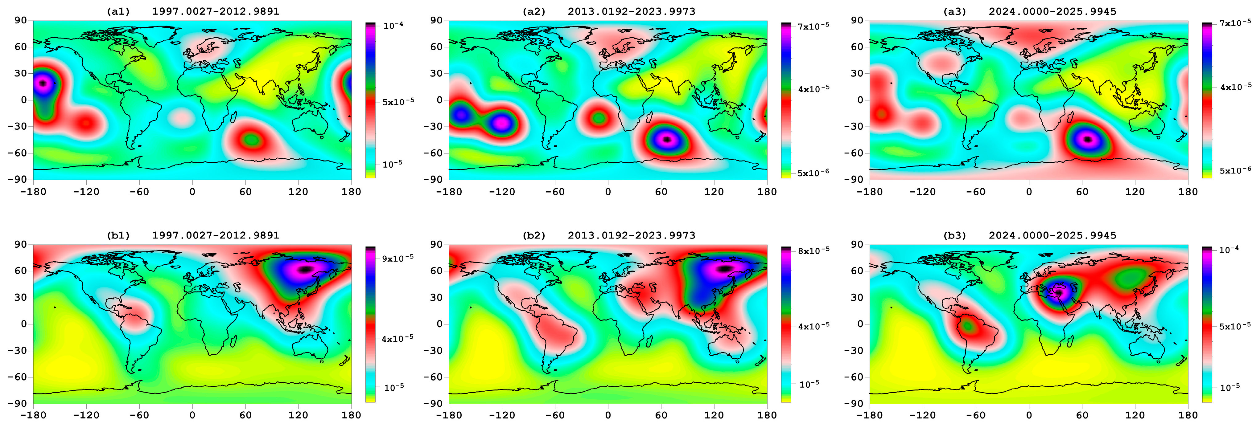
Figure 5 presents the averaged distribution maps of extreme seismic noise properties for the two cases, $({\gamma }_{\min },\Delta {\alpha }_{\min },E{n}_{\max })$ and $({\gamma }_{\max },\Delta {\alpha }_{\max },E{n}_{\min })$, for three consecutive time intervals. The first interval covers the time interval from the beginning of observations to the time of the Tohoku mega-earthquake in Japan on 11 March 2011. The next time interval extends from the Tohoku event to the end of 2024. The final time interval begins in early 2024 and extends until the end of 2025. The final time interval, the shortest, was chosen because it contains a sharp increase in the number of pairs of control points with correlations exceeding the 0.8 threshold (Figure 3b).

As can be seen in Figure 5(a1–a3), the concentration regions of the most “quiet” seismic noise behavior (variant $({\gamma }_{\min },\Delta {\alpha }_{\min },E{n}_{\max })$) are stable throughout the entire observation interval, with the exception of the middle of the Atlantic Ocean in the vicinity of the island of Saint Elena and the south of the Indian Ocean in the vicinity of the Kerguelen archipelago, where a gradual increase in probability density is observed. As for the variant $({\gamma }_{\max },\Delta {\alpha }_{\max },E{n}_{\min })$ of the most “violent” seismic noise behavior, the concentration region of this behavior remains stable until 2024 and occupies northeastern Eurasia, centered on the Putarana Plateau, which formed after the largest supervolcanic eruption 250 million years ago. However, after 2024, this region shifted to the Middle East.

We currently lack a definitive explanation for this effect. The only hypothesis is that the Kamchatka mega-earthquake of 29 July 2025 had an unexpectedly strong impact on the seismic noise field, unlike previous mega-earthquakes: Sumatra (26 December 2004, M = 9.1), Maule (Chile) (27 February 2010, M = 8.8), and Tohoku (Japan) (11 March 2011, M = 9.1).

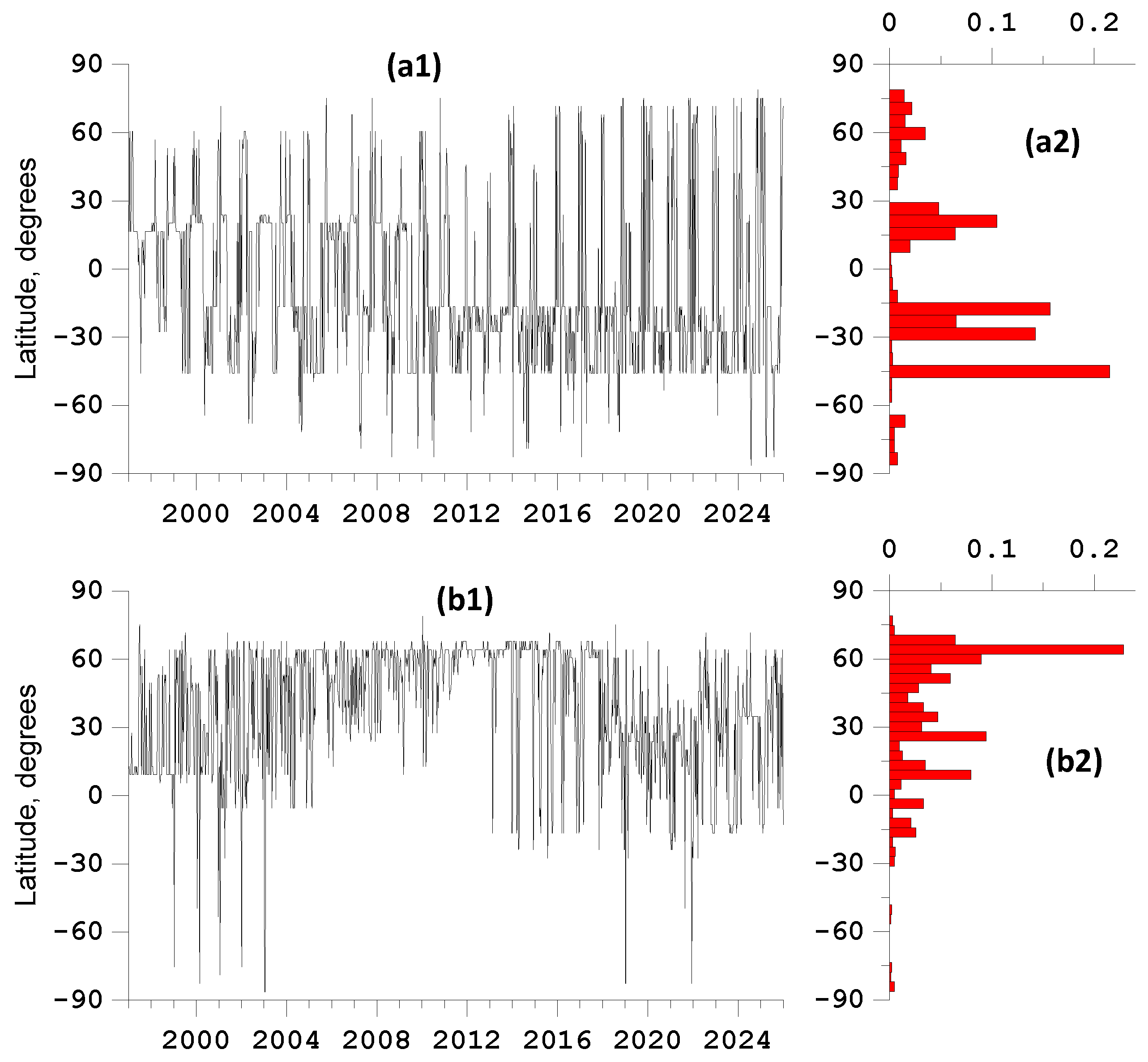
The graphs in Figure 6 provide a more detailed representation of the spatiotemporal features of the changes in the distribution densities of the extreme values of seismic noise properties. The graphs in Figure 6(a1,b1) represent the changes in the latitude of those nodes of a regular 100 × 50 grid for which the maximum distribution of extreme properties is realized for the cases $({\gamma }_{\min },\Delta {\alpha }_{\min },E{n}_{\max })$ and $({\gamma }_{\max },\Delta {\alpha }_{\max },E{n}_{\min })$.

Figure 6(a1) shows a strong annual periodicity, with the point of maximum probability density $({\gamma }_{\min },\Delta {\alpha }_{\min },E{n}_{\max })$ making a sudden transition to the Arctic region in December–January. Furthermore, Figure 6(a1) shows a transition from the point of maximum probability density from 15 degrees north latitude to 30 degrees south latitude, occurring around 2011, which is noticeable when comparing Figure 5(a1,a2).

As for Figure 6(b1), it shows a gradual evolution of the region of maximum probability densities for the case $({\gamma }_{\max },\Delta {\alpha }_{\max },E{n}_{\min })$ from northeastern Eurasia to the Middle East, which began around 2019.

Figure 6(a2,b2) present graphs of probability histograms of the corresponding latitude values with maximum values of the distribution densities of extreme values of noise properties.

6. Sequence of Major Earthquakes and Their Periodic Components

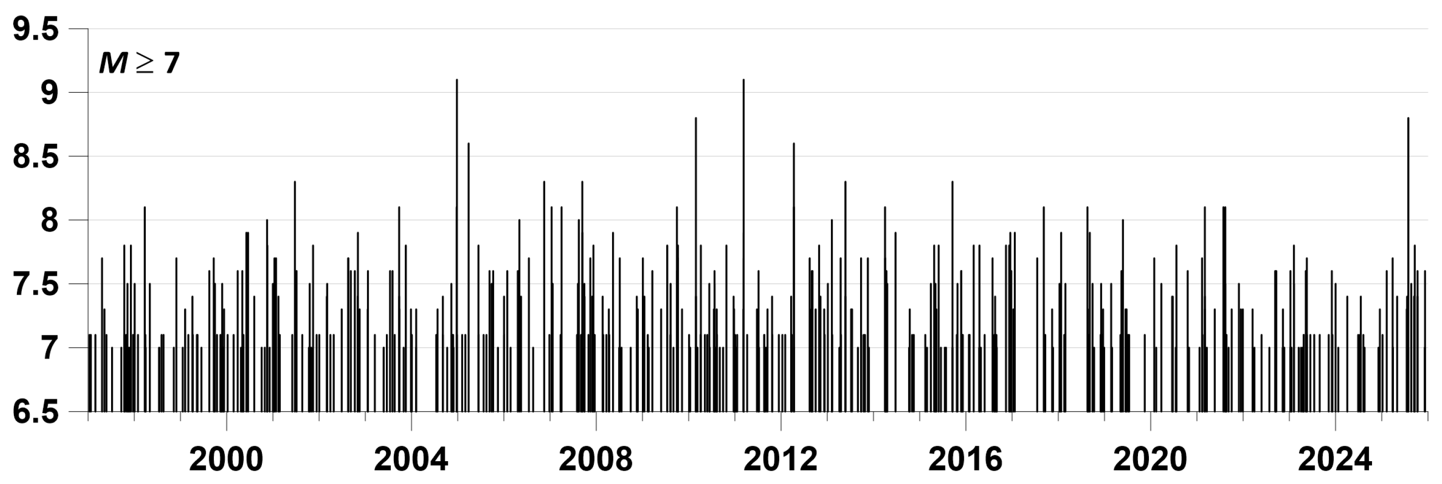
The following sections of the article analyze the relationships between the properties of global seismic noise and the sequence of strong earthquakes. Figure 7 shows the time sequence of 433 seismic events with a magnitude of at least 7 for the time interval 1997–2025.

As Figure 7 shows, the regime of the strongest earthquakes is non-stationary. In particular, we are interested in the periodic components of the intensity change in the earthquake sequence. In [39,40], this method was used to calculate the periodic component of the stepwise variations in the time series of the displacement of the Earth’s surface, which was measured by GPS, and periodic components of earthquake sequences.

Let us consider the sequence of time moments $t_i,i=1,\dots ,N$ on the interval $(0,T]$. Consider the following intensity model containing a periodic component:

$$\lambda (t)=\mu \cdot (1+a\cos (2\pi t/\eta +\phi ))$$

(9)

where period $\eta$, amplitude $a,0\le a\le 1$, phase angle $\phi \in [0,2\pi ]$, and multiplier $\mu >0$ (describing the Poisson part of the intensity) are parameters of the model. Thus, the Poisson part of the intensity is modulated by a harmonic oscillation. Let us fix some value of period $\eta$. The logarithmic likelihood function [41], in this case for a series of observed events, is equal to:

$$\begin{array}{l}\ln L(\mu ,a,\phi |\eta )={\displaystyle \sum _i\ln (\lambda (t_i))}-{\displaystyle {\int }_0^T\lambda (s)ds}=\\ =N\ln (\mu )+{\displaystyle \sum _i\ln (1+a\cos (2\pi t_i/\eta +\phi ))}-\mu T-{\displaystyle \frac{\mu a\eta }{2\pi }}[\sin (2\pi T/\eta +\phi )-\sin (\phi )]\end{array}$$

(10)

Taking the maximum of expression (10) with respect to the parameter $\mu$, it is easy to find that

$$\ln (L(\widehat{\mu },a,\phi |\eta ))={\displaystyle \sum _i\ln (1+a\cos (2\pi t_i}/\eta +\phi ))+N\cdot \ln (\widehat{\mu }(a,\phi |\eta ))-N$$

(11)

where $\widehat{\mu }(a,\phi |\eta )=N/[T+{\displaystyle \frac{a\eta }{2\pi }}\cdot ((\sin (2\pi T/\eta +\phi )-\sin \phi ))]$.

Expression $\widehat{\mu }(a=0,\phi |\eta )\equiv {\mu }_0=N/T$ is an estimate of the intensity of the process under the condition that it is purely random. The increment of the logarithmic likelihood function with respect to a purely random sequence is equal to

$$\Delta \ln L(a,\phi |\eta )={\displaystyle \sum _i\ln (1+a\cos (2\pi t_i/\eta }+\phi ))+N\cdot \ln (\widehat{\mu }(a,\phi |\eta )/{\mu }_0)$$

(12)

Let

$$R(\eta )=\underset{a,\phi }{\max }\Delta \ln L(a,\phi |\eta ),\hspace{1em}0\le a\le 1, \phi \in [0,2\pi ]$$

(13)

For a fixed value of period $\eta$, we consider two competing models of earthquake sequences: the simplest model of a stationary Poisson process, which is described by one parameter ${\mu }_0$ of average intensity, and a more complex model (9), containing three parameters $(\mu ,a,\phi )$. The difference between the maximum values of the log-likelihood function for the complex data model (9) and the simple Poisson process model is always non-negative and gives a measure of how much more “profitable” the complex model is compared to the simple one. According to Wilks’s theorem [35], this difference is asymptotically distributed as ${\mathsf{\chi }}_{\mathrm{m}}^2$, where the number of degrees of freedom $\mathrm{m}$ is equal to the difference between the number of parameters of the competing models, that is, in our case, $\mathrm{m}=2$, and the asymptotic distribution of the difference $\Delta \ln L$ in the maximum values of the likelihood functions is ${\mathsf{\chi }}_2^2$. Since the distribution ${\mathsf{\chi }}_2^2$ coincides with the exponential distribution, we obtain the following asymptotic distribution:

$$\mathrm{P}(R(\eta )<x)=1-e^{-x},\hspace{1em}N\to \infty$$

(14)

Expression (14) provides the possibility to find thresholds for statistics (14) that allow us to find when the hypothesis of the existing periodical component of intensity with a given period $\eta$ could be accepted.

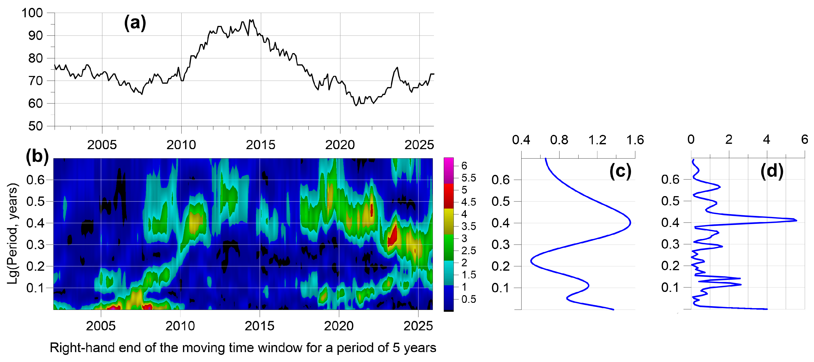
For a time sequence of seismic events with a magnitude of at least 7, we calculated the increments of the logarithmic likelihood function (13) in a sliding time window of 5 years with a shift of 0.01 years for 100 period values $\eta$ corresponding to the values varying from 1 to 5 years with a uniform step in a logarithmic scale. The number of events within the moving time window of the period of 5 years is presented in Figure 8a. The average number of events within the sliding window is 75, and it varies from 59 to 97. Therefore, we believe that the conditions of the asymptotic inequality (13) are applicable. It is interesting to note in Figure 8a that the number of events $M\ge 7$ in the 5-year time window started to increase after the Maule mega-earthquake in Chile on 27 February 2010, M = 8.8, and reached its maximum values after the Tohoku mega-earthquake in Japan on 11 March 2011, M = 9.1.

The resulting time–frequency dependence is shown in Figure 8b. Figure 8c shows a plot of the mean values of the log-likelihood increments for all 5-year time windows. It shows a spectral peak at a period of 2.6 years. This plot was obtained by summing all time windows, and the maximum increment value $\Delta \ln L$ is 1.55, which gives a probability of 0.787 for accepting the hypothesis of the presence of a periodic intensity component for a period of 2.6 years, according to Equation (14). However, if we calculate the value $\Delta \ln L$ using the entire sample of seismic event times, we obtain the plot shown in Figure 8d, in which the maximum value $\Delta \ln L$ at a period of 2.6 years is 5.55, which gives a probability of accepting the periodicity hypothesis of 0.996.

To determine the dominant period in the earthquake sequence, one could rely solely on the graph in Figure 8d. However, the time–frequency diagram in Figure 8b is of independent interest, as it provides information on the evolution of the periodic intensity components. It shows that the period gradually increases until approximately 2013, after which the periodic component virtually disappears until 2018. After 2018, two branches of the periodic component’s evolution emerge—low-frequency and high-frequency—which merge at the end of the analyzed time interval.

An analysis of the periodic components of the seismic process yielded an interesting result: it turned out that the dominant period of seismicity, 2.6 years, is very close to the 2.57-year period of oscillations of the average value of pairwise absolute correlations between the properties of seismic noise at reference points—Figure 3(a2).

Although Figure 8b demonstrates the variability in the spectral composition of the sequence of the strongest earthquakes, it is nonetheless clear that the 2.6-year oscillation period (logarithm equals 0.4) is dominant starting from the 2008 timestamp of the right-hand end of the 5-year sliding time window. Given the 5-year window period, this means that this period began to dominate starting in 2003, that is, approximately from the time when the trend in Figure 3(a1) changed with superposed oscillations for a period of 2.57 years.

7. Weighted Means of Seismic Noise Properties and Their Local Extrema

We apply the method for calculating weighted averages (“W-averaging” in Equations (5) and (6)) to the analyzed seismic noise statistics. The weights for averaging are the squared absolute values of the first eigenvectors of the 50 × 50 correlation matrices calculated for daily values of seismic noise properties ${\tilde{\mathsf{\gamma }}}_j(t)$, $\Delta {\tilde{\mathsf{\alpha }}}_j(t)$, $\tilde{E}{n}_j(t)$ at 50 reference points, corresponding to the maximum eigenvalues of these matrices. The weighted average values of these properties of seismic noise, calculated in a sliding time window of 365 days, are denoted by $W_{\gamma }(t)$, $W_{\Delta \alpha }(t)$ and $W_{En}(t)$. 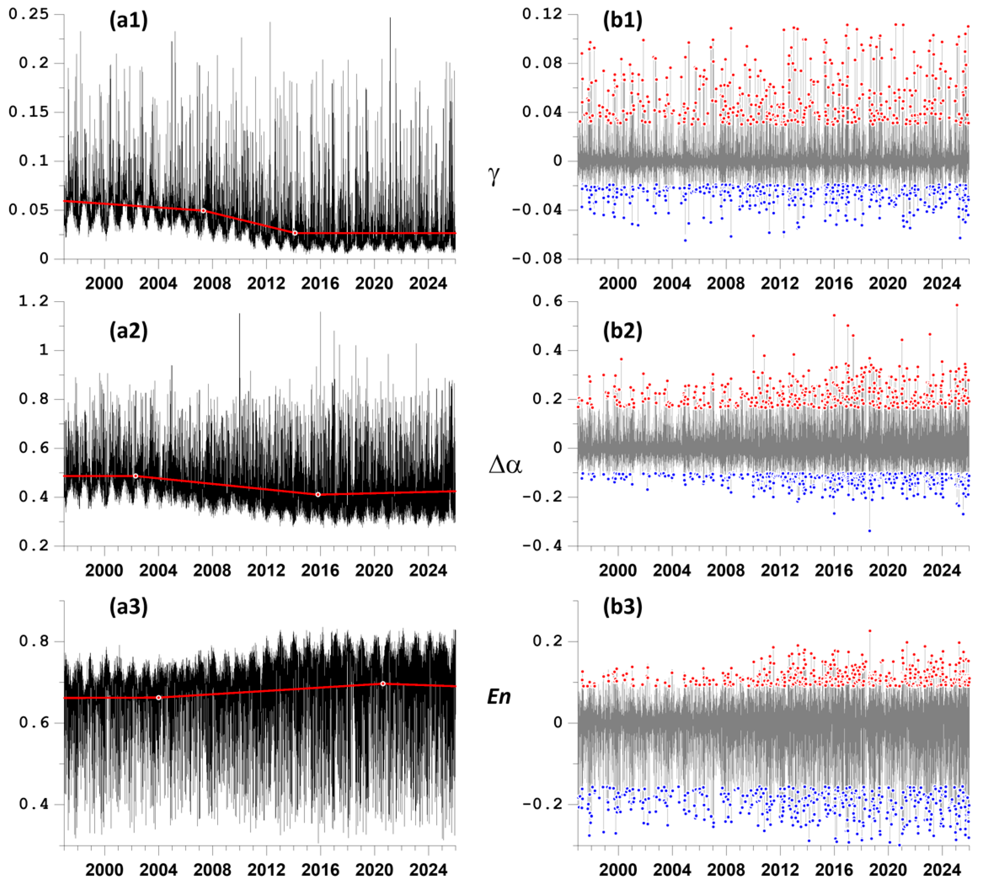The results of such a “left-oriented” weighted “W-average” are presented in Figure 9(a1–a3). These graphs show that the behavior of the first principal components of the analyzed properties of seismic noise can be divided into three large time fragments, of which the middle fragments (time stamp intervals 2007.33–2014.12 (1 May 2007–13 February 2014) for $W_{\gamma }(t)$, 2002.31–2015.81 (24 April 2002–23 October 2015) for $W_{\Delta \alpha }(t)$, and 2004–2020.62 (1 January 2004–14 August 2020) for $W_{En}(t)$) correspond to transient processes of change in the average values.

In the future, we will be interested in the positions of the time points of a certain number of the largest local maxima or the smallest local minima of daily seismic noise properties in comparison with the times of earthquakes with a magnitude of at least 7 (Figure 7). To eliminate the influence of low-frequency components of changes in statistical values on the determination of the times of local extrema, the time series of noise properties were subjected to the operation of removing low frequencies using Gaussian kernel smoothing. Let $z(t)$ be a time series with discrete time $t$. Gaussian kernel averaging of a time series $z(t)$ with radius (scale parameter) $a>0$ at time $t$, is calculated using the formula [42]:

$$\overline{z}(t|a)={\displaystyle \sum _{\xi }z(\xi )\cdot e^{-{\left(\frac{\xi -t}{a}\right)}^2}}/{\displaystyle \sum _{\xi }{e}^{-{\left(\frac{\xi -t}{a}\right)}^2}}$$

(15)

Since the Gaussian smoothing kernel used in Equation (15) is symmetrical about zero, the position of the local extremum identified after local trend removal in the vicinity of a radius of two samples is unbiased. The local trend removal operation itself, due to the rapid decay of the Gaussian kernel, is a “local” operation, the result of which is influenced by the behavior of the original signal in the vicinity of each point, the radius of which is approximately equal to two samples.

Let us denote $W_{\gamma }^{(a)}(t)$, $W_{\Delta \alpha }^{(a)}(t)$, and $W_{En}^{(a)}(t)$ as the result of removing the local trends from the signals $W_{\gamma }(t)$, $W_{\Delta \alpha }(t)$, and $W_{En}(t)$ by the Gaussian window of radius $a$, equal to 2 days. We are interested in the local extremum points of signals $W_{\gamma }^{(a)}(t)$, $W_{\Delta \alpha }^{(a)}(t)$, and $W_{En}^{(a)}(t)$. The results of removing local trends and determining local extremum points are presented in Figure 9(b1–b3). From the most prominent local extrema, the number 433, representing the most prominent local extrema, was chosen as equal to the number of earthquakes with magnitudes not less than 7.

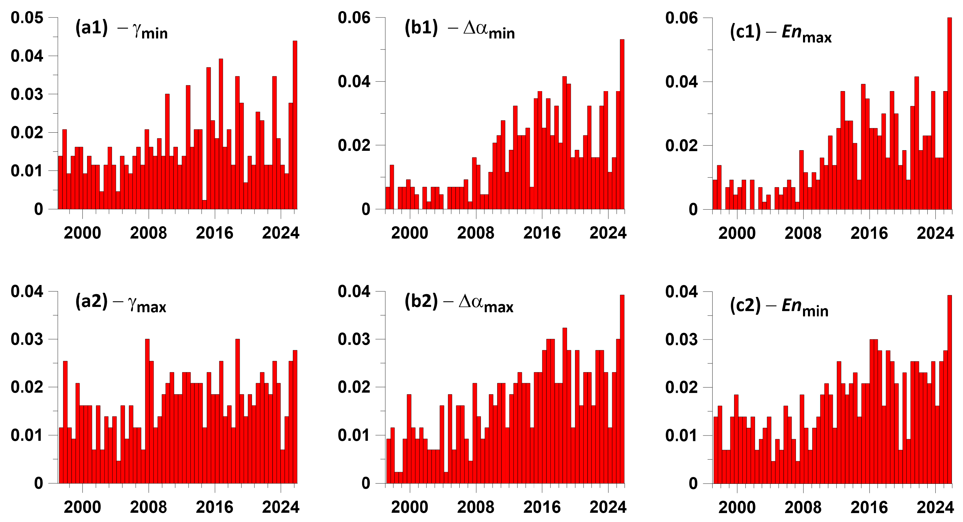
Let us analyze how the time points of the most significant local extrema of the statistics $W_{\gamma }^{(a)}(t)$, $W_{\Delta \alpha }^{(a)}(t)$, and $W_{En}^{(a)}(t)$ are distributed. To do this, let us calculate the probability histograms separately for 433 of the smallest local minima $W_{\gamma }^{(a)}(t)$, $W_{\Delta \alpha }^{(a)}(t)$ and 433 of the largest local maxima of entropy $W_{En}^{(a)}(t)$ (which means case $({\gamma }_{\min },\Delta {\alpha }_{\min },E{n}_{\max })$), i.e., empirical probabilities of time values falling within successive six-month intervals. Since the total observation time is 29 years, the number of such intervals is 58. Figure 10(a1–c1) show graphs of these histograms. Figure 10(a2–c2) correspond to probability histograms for 433 of the largest local maxima $W_{\gamma }^{(a)}(t)$, $W_{\Delta \alpha }^{(a)}(t)$ and 433 of the smallest local minima of entropy $W_{En}^{(a)}(t)$ (case $({\gamma }_{\max },\Delta {\alpha }_{\max },E{n}_{\min })$). It shows that the last six-month interval has the highest empirical probability of containing local extremum points, except Figure 10(a2).

Thus, from the graphs in Figure 10, it is evident that the times of prominent local extremes of almost all seismic noise statistics are significantly concentrated in the second half of 2025.

8. Influence Matrices

Further analysis involves calculating a measure describing the lead or lag of two time sequences, one of which represents the times of strong earthquakes, and the other represents the times of certain characteristic features of seismic noise statistics. Such features could be, for example, the times of the most prominent local extrema.

To solve this problem, we apply the influence matrices method, which was used in [43,44,45,46] to analyze the prognostic properties of the Earth’s surface tremors, measured by GPS, to analyze the relationship between magnetic field fluctuations and strong earthquakes, and to analyze the relationship between anomalies in meteorological time series and seismicity.

Let $t_j^{(p)},j=1,\dots ,N_p; p=1,2$ represent the moments of time of two sequences of events. Let us represent their intensities as follows:

$${\mu }^{(p)}(t)=b_0^{(p)}+{\displaystyle \sum _{q=1}^2{b}_q^{(p)}}\cdot g^{(q)}(t)$$

(16)

where $b_0^{(p)}\ge 0,b_q^{(p)}\ge 0$ are parameters, $g^{(q)}(t)$ is the influence function of time moment $t_j^{(q)}$ from the sequence with number $q$:

$$g^{(q)}(t)={\displaystyle {\sum }_{t_j^{(q)}<t}{e}^{-(t-t_j^{(q)})/\tau }}$$

(17)

The parameter $\tau$ is a characteristic of the decay time of the weight of the event with number $j$ for $t>t_j^{(q)}$.

The strength of the mutual influence of the sequence $q$ on the flow $p$ is defined by the parameter $b_q^{(p)}$. The self-exciting effect is determined by the parameter $b_p^{(p)}$. The parameter $b_0^{(p)}$ reflects a purely random (Poisson) component of intensity. Let us fix the parameter $\tau$ and consider the problem of determining the parameters $b_0^{(p)},b_q^{(p)}$.

The log-likelihood function for the model of intensity (16) equals [41]:

$$\ln (L_p)={\displaystyle \sum _{j=1}^{N_p}\ln ({\mu }^{(p)}(t_j^{(p)}))-{\displaystyle \underset{0}{\overset{T}{\int }}{\mu }^{(p)}(s)ds}},\hspace{1em}p=1,2$$

(18)

The parameters $b_0^{(p)},b_q^{(p)}$ should be found by maximizing (18). As shown in detail in [13,43,44,45,46], the problem of finding the parameter values $b_0^{(p)},b_q^{(p)}$ from the maximum likelihood principle is reduced to solving problems for the maximum:

$${\displaystyle \sum _{j=1}^{N_p}\ln ({\mu }_0^{(p)}+{\displaystyle \sum _{q=1}^2{b}_q^{(p)}\cdot \Delta g^{(q)}(t_j^{(p)}))\to }}\underset{b_1^{(p)},b_2^{(p)}}{\max },\hspace{1em}p=1,2$$

(19)

where ${\mu }_0^{(p)}=N_p/T$, $\Delta g^{(\beta )}(t)=g^{(\beta )}(t)-{\overline{g}}^{(\beta )}$, ${\overline{g}}^{(q)}={\displaystyle {\int }_0^T{g}^{(q)}(s)ds}/T$, under restrictions:

$$b_1^{(p)}\ge 0,\hspace{1em}{b}_2^{(p)}\ge 0,\hspace{1em}{b}_1^{(p)}{\overline{g}}^{(1)}+b_2^{(p)}{\overline{g}}^{(2)}\le {\mu }_0^{(p)}$$

(20)

For a given relaxation time $\tau$, the problem (19) and (20) is solved numerically. The elements of the influence matrix ${\kappa }_q^{(p)},p=1,2;\hspace{1em}q=0,1,2$ could be defined as:

$${\kappa }_0^{(p)}=b_0^{(p)}/{\mu }_0^{(p)}\ge 0,\hspace{1em}{\kappa }_q^{(p)}=b_q^{(p)}\cdot {\overline{g}}^{(q)}/{\mu }_0^{(p)}\ge 0$$

(21)

The quantity ${\kappa }_0^{(p)}$ is a pure random share of the intensity ${\mu }_0^{(p)}$ of the process $p$. The share ${\kappa }_p^{(p)}$ reflects the self-excitation, whereas ${\kappa }_q^{(p)},p\ne q$ describes the external influence $q\to p$. The normalization condition follows from (21):

$${\kappa }_0^{(p)}+{\kappa }_1^{(p)}+{\kappa }_2^{(p)}=1,\hspace{1em}p=1,2$$

(22)

The influence matrix is defined as follows:

$$\left(\begin{array}{l}{\kappa }_0^{(1)} {\kappa }_1^{(1)} {\kappa }_2^{(1)}\\ {\kappa }_0^{(2)} {\kappa }_1^{(2)} {\kappa }_2^{(2)}\end{array}\right)$$

(23)

The sum of the component rows of the influence matrix (23) equals 1. The matrix is estimated in a moving time window of a certain period for a given value of the relaxation time $\tau$.

We investigate the combined effect of the advance or lag of the local extrema of the functions $W_{\gamma }^{(a)}(t)$, $W_{\Delta \alpha }^{(a)}(t)$, and $W_{En}^{(a)}(t)$ relative to the earthquake moments. To do this, we calculate the first principal component of these functions in a sliding time window of 365 days according to Equations (1)–(6) for the P-averaging and denote it by $P_{\gamma ,\Delta \alpha ,En}^{(Wa)}(t)$.

The components of the influence matrix (23) are calculated in a sliding time window of 2.6 years with an offset of 0.01 years. This choice of window length is due to the fact that it is equal to the dominant period of the sequence of strong earthquakes (Figure 8).

The parameter $\tau$ is searched by maximizing the average value of the difference $\Delta \kappa ={\kappa }_2^{(1)}-{\kappa }_1^{(2)}\to \underset{\tau }{\max }$, where ${\kappa }_2^{(1)}$ is the share of the intensity of the earthquake sequence caused by the “influence” of the sequence of local extrema, and ${\kappa }_1^{(2)}$ is the share of the intensity of the local extrema sequence caused by the leading influence of seismic events.

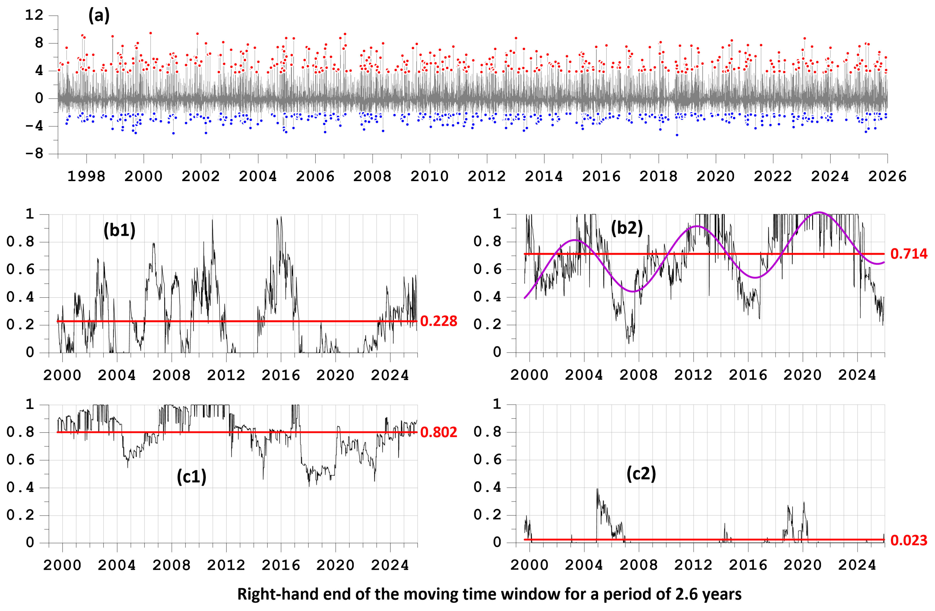
The graphs in Figure 11 show that the local minima of the function $P_{\gamma ,\Delta \alpha ,En}^{(Wa)}(t)$ lead earthquake times significantly more than vice versa (average lead measures are 0.714 versus 0.228). Moreover, the lead measure of the local minima $P_{\gamma ,\Delta \alpha ,En}^{(Wa)}(t)$ relative to seismic event times is subject to cyclic variations with a period of about 9 years, as can be seen in Figure 11(b2). The cyclic trend in Figure 11(b2) (purple line) is determined by minimizing the variance of the residual using a trial cyclic trend with fitted parameters of the linear trend and oscillation period. As for the local maxima of the function $P_{\gamma ,\Delta \alpha ,En}^{(Wa)}(t)$, they almost always occur after earthquakes, and the reverse effect is negligible (the mean lag measure is 0.802 versus 0.023).

9. The Step Component of the Entropy Probability Density and Its Relationship with the Strongest Earthquakes

The number of grid nodes covering the surface of the Earth equals $M=100\times 50=50,000$. Let us calculate the histogram of the weighted probability density functions (PDFs) for each 10-day interval $i$ as a sequence of values:

$$g_k^{(i)}=l_k^{(i)}/L_b,\hspace{1em}k=1,\dots ,L_b$$

(24)

Here $L_b$ is the number of bins dividing the range of density variation within a given 10-day window into intervals of equal length, $l_k^{(i)}$ is the number of PDF values within the interval with number $k$. We choose the value $L_b=\sqrt{M}$ according to [36,42]. It is evident that ${\displaystyle {\sum }_k{g}_k^{(i)}=1}$. Thus, values of the histogram (24) have the properties of a discrete probability distribution. The normalized entropy of this distribution is calculated as:

$${\mathrm{E}}_i=-{\displaystyle \sum _{k=1}^{L_b}{g}_k^{(i)}\ln (g_k^{(i)})/\ln (L_b),\hspace{1em}0\le {\mathrm{E}}_i\le 1}$$

(25)

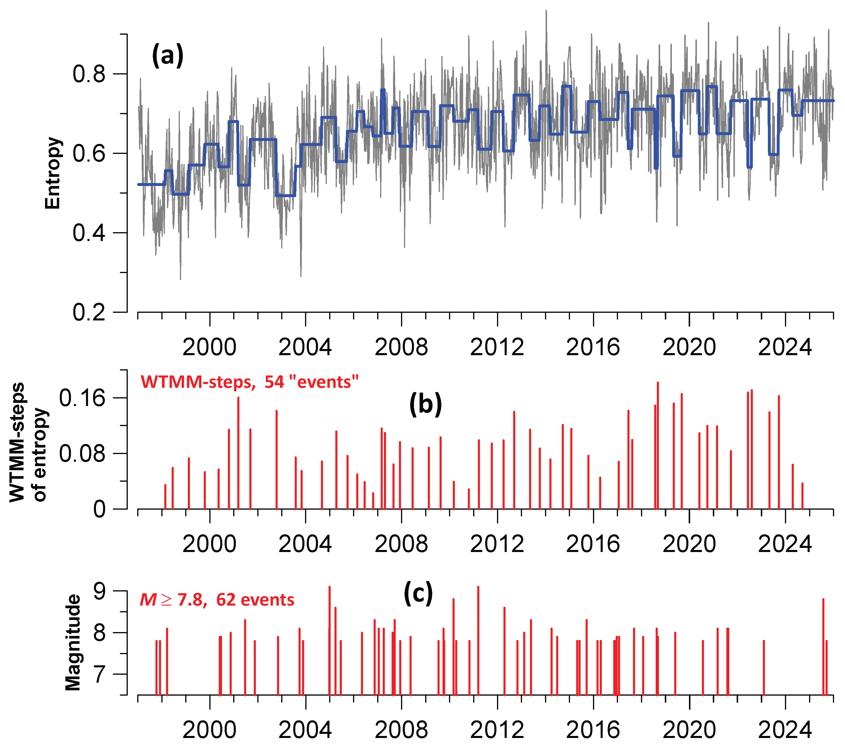
The plot of entropy change (25) is indicated by the gray line in Figure 12a.

The behavior of entropy (25) in short time intervals of 10 days is non-stationary. We are interested in points where the average entropy value changes significantly. To identify such time points, we apply the Wavelet Transform Modulus Maxima (WTMM) method, which allows us to formalize the determination of significant changes in the average value of a noisy signal using sufficiently long chains of the local maxima of the wavelet transform modulus over time, depending on the scale of temporal changes under consideration. The method for determining jumps in the average level is based on the construction of a piecewise-step approximation of the signal under study. This approximation is constructed using continuous wavelet transforms with a kernel in the form of derivatives of a Gaussian function, which allows one to formalize the selection of moments in time at which a significant, scale-dependent change in the mean value of a noisy signal occurs [46,47].

Let us define the smoothed functions of entropy (25):

$$\overline{\mathrm{E}}(t,a)={\displaystyle \sum _{\xi }{\mathrm{E}}_{\xi }\cdot e^{-{\left(\frac{\xi -t}{a}\right)}^2}}/{\displaystyle \sum _{\xi }{e}^{-{\left(\frac{\xi -t}{a}\right)}^2}}$$

(26)

In Equation (26), a Gaussian function is used as the smoothing kernel, with the parameter $a>0$ being the smoothing radius. Due to the rapid decay of the Gaussian function and its symmetry, the first derivative of the smoothed entropy can be written in the form:

$${\overline{\mathrm{E}}}^{\prime }(t,a)=2\cdot {\displaystyle \sum _{\xi }{\mathrm{E}}_{\xi }\cdot \left(\frac{\xi -t}{a}\right)\cdot e^{-{\left(\frac{\xi -t}{a}\right)}^2}}/{\displaystyle \sum _{\xi }{e}^{-{\left(\frac{\xi -t}{a}\right)}^2}}$$

(27)

We define a WTMM point $t_a$ as the argument of the modulus $|{\overline{\mathrm{E}}}^{\prime }(t,a)|$ at which a local maximum is achieved with respect to $t$. As the smoothing parameter $a$ changes, the points $t_a$ on the plane $(t,a)$ form so-called WTMM chains. The set of all WTMM chains forms the WTMM skeleton of the signal. Since ${\overline{\mathrm{E}}}^{\prime }(t,a)=d\overline{\mathrm{E}}(t,a)/dt$, the points $t_a$ determine the time instants for which the maximum trends (decrease or increase) of the smoothed function $\overline{\mathrm{E}}(t,a)$ are observed. If we set a parameter $a=a^{*}$, a sequence of WTMM points $t_{a^{*}}^{(k)}$ will arise, from which we can formalize a stepwise approximation of the original signal $\mathrm{E}(t)$ as a sequence of its average values between adjacent time instants $t_{a^{*}}^{(k)}$ and $t_{a^{*}}^{(k+1)}$.

Let us consider the sequence of time instants of stepwise changes in the WTMM approximation of entropy (25) of the values of the weighted average density distribution of extreme values $({\gamma }_{\min },\Delta {\alpha }_{\min },E{n}_{\max })$. Figure 12a shows a graph of the change in this entropy (gray line) and a graph of the stepwise WTMM approximation. Since entropy (25) is defined as a sequence of values with a time step of 10 days, then when selecting a parameter $a^{*}=10$, the dimensional length of this parameter is equal to 100 days.

Figure 12b shows the time sequence of the absolute values of steps in the WTMM approximation. We examine the relationship between steps in the WTMM approximation of entropy and the time instants of the strongest earthquakes with a magnitude of at least 7.8, which is shown in Figure 12c.

Let us calculate the influence matrix between the two time sequences shown in Figure 12b,c over the entire length of the available sample. The result depends on the choice of the parameter $\tau$, which we select based on the condition of maximizing the difference between the influence matrix components responsible for mutual influence. This value is $\tau =0.45$ years. The calculation results are presented in

Table 1. Influence matrix between time moment sequences of the WTMM steps of the weighted average probability density function of the extreme case $({\gamma }_{\min },\Delta {\alpha }_{\min },E{n}_{\max })$ in successive 10-day time intervals and the sequence of earthquakes with a magnitude not less than 7.8 for $\tau =0.45$ years.

	Poisson	WTMM Steps	EQ $\mathit{M}\mathbf{\ge }\mathbf{7.8}$
WTMM steps	0.973	0.000	0.027
EQ $M\ge 7.8$	0.618	0.382	0.000

.

The results presented in the Table 1 indicate that the abrupt changes in the entropy values of the weighted average probability densities of the extreme value distributions for the case $({\gamma }_{\min },\Delta {\alpha }_{\min },E{n}_{\max })$ significantly precede the times of the strongest earthquakes (the lead measure is 0.382 versus 0.027). It is interesting to note that, when similarly considering the “antagonistic” case $({\gamma }_{\max },\Delta {\alpha }_{\max },E{n}_{\min })$, the mutual influence is negligible.

10. Estimates of Coherence

To analyze the relationships between the length of day time series reflecting the irregularity of the Earth’s rotation and the properties of seismic noise, we need to calculate the quadratic coherence between two time series in a sliding time window. For this purpose, we use a 2-dimensional autoregressive model, which provides high-resolution spectral analysis for short time samples [48]. For a 2-dimensional time series $X(t)=(X_1(t),X_2(t))$, the AR model is described by the formula:

$$X(t)+{\displaystyle \sum _{k=1}^p{B}_k\cdot }X(t-k)=\epsilon (t)$$

(28)

Here $p$ is the autoregression order, $B_k$ are matrices of autoregression coefficients of the size $2\times 2$, and $P=M(\epsilon (t){\epsilon }^T(t))$ is the covariance matrix of the size $2\times 2$ of residual signal $\epsilon (t)$. For fast computing of matrices $B_k$ and $P$, the Durbin–Levinson procedure is applied [49]. The spectral matrix estimate is defined by the formula:

$$S_{XX}(\omega )={\mathsf{\Phi }}^{-1}(\omega )\cdot P\cdot {\mathsf{\Phi }}^{-H}(\omega ),\hspace{1em}\mathsf{\Phi }(\omega )=E+{\displaystyle \sum _{k=1}^p{B}_k}{e}^{-i\omega k}$$

(29)

where $E$ is a unit matrix of the size $2\times 2$, $\omega$ is a frequency (in units $2\pi /\Delta t$, where $\Delta t$ is the time step, 1 day in our case, $0<\omega <\pi /\Delta t$), and “$H$” is a symbol of Hermitian conjugation. Squared coherence spectrum is computed by the formula:

$$c^2(\omega )=|S_{12}(\omega ){|}^2/S_{11}(\omega )\cdot S_{22}(\omega )$$

(30)

Here $S_{11}(\omega )$ and $S_{22}(\omega )$ are diagonal elements of the matrix (29), whereas $S_{12}(\omega )$ is the cross-spectrum.

11. Connection of Seismic Noise Response to the Irregularity of Earth’s Rotation with Major Earthquakes

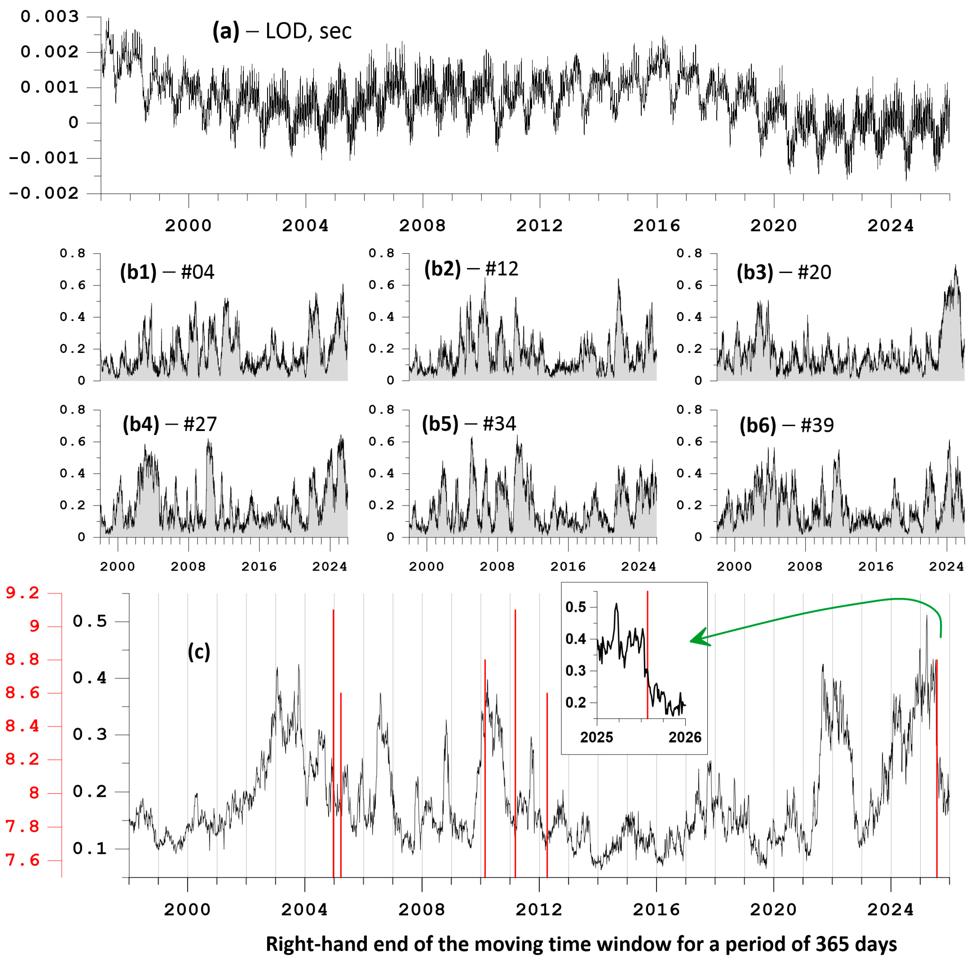
The connection between the irregularity of the Earth’s rotation measured by the length of day (LOD) and seismicity was analyzed in [50]. The trigger mechanism of the effect of variations in the Earth’s rotation on the seismic process was studied in [51]. Estimates of the effect of a strong earthquake on the length of the day are given in [52]. Figure 13a presents the length of day time series for the interval 1997–2025 [53].

The relationship between seismic noise properties and irregularity of the Earth’s rotation was investigated in [13]. We calculated the maximum quadratics coherence spectrum between the LOD and the first principal component of properties $P_{\mathsf{\gamma },\Delta \mathsf{\alpha },En}^{(j)}(t)$ for each of 50 reference points in a moving time window of 365 days with a mutual shift of 3 days. We call these maximum quadratic coherences as the response $R_{\mathsf{\gamma },\Delta \mathsf{\alpha },En}^{(j)}(t)$ of seismic noise to the LOD. We used a 2-dimensional AR-model (28) for $p=5$ within a moving time window of 365 days with a mutual shift of 3 days.

Examples of such response functions are presented in Figure 13(b1–b6) for six reference points. Having response functions $R_{\mathsf{\gamma },\Delta \mathsf{\alpha },En}^{(j)}(t)$ from all reference points, we calculated their weighted mean value where we used squared components of the first eigenvector (corresponding to the maximum eigenvalue) of the 50 × 50 size covariance matrix. This weighted mean of all response functions we will call the integral response of three seismic noise properties all over the world to the irregularity of the Earth’s rotation.

Figure 13c of the integrated response of seismic noise properties to the Earth’s rotation irregularity shows that the strongest earthquakes $M\ge 8.5$ occur primarily after the response reaches its maximum. This response behavior highlights a distinctive pattern before and after the Kamchatka mega-earthquake of 29 July 2025, $M=8.8$ [37,38]: a prolonged increase prior to the event and a sharp decline immediately afterward.

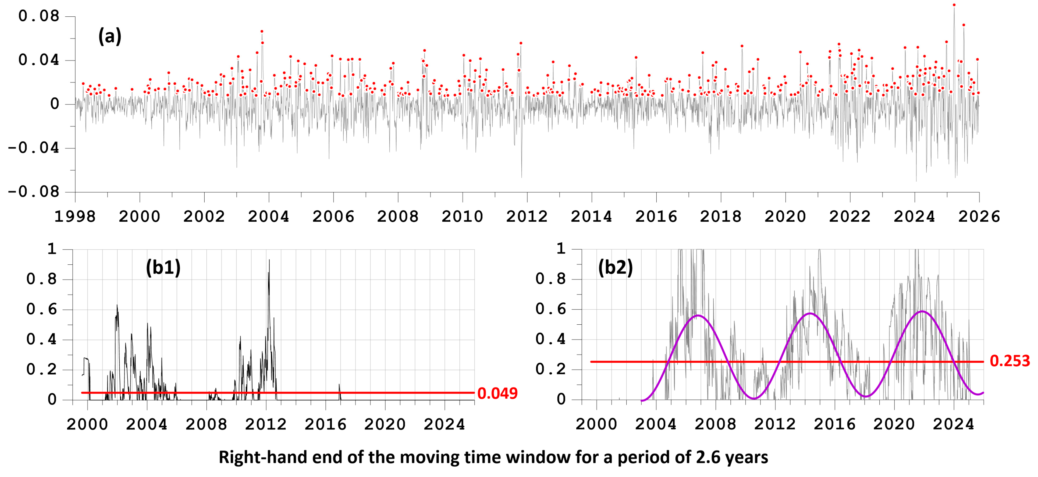
To analyze the relationship between local extrema of the integrated seismic noise response to the LOD and seismic events $M\ge 7$, we remove local trends from the response function using a Gaussian window. The goal of this operation, as before, is to isolate the effect of the leading time of the most prominent local extrema relative to the earthquake time points. However, it turned out that the optimal window width, for which the leading effect in this case is maximal, is 24 days (eight time steps with a step length of 3 days). Figure 14a shows the response function graphs after removing local trends and the positions of the 433 largest local maxima. Figure 14(b1,b2) show graphs of the change in the influence matrix components responsible for the mutual leading of the analyzed time sequences. The assessments were performed in a sliding time window of 2.6 years with an offset of 0.01 years. The relaxation time value $\tau$ was chosen to maximize the difference between the “forward” and “reverse” lead measures. This value turned out to be equal to $\tau =0.148$ year.

Comparing the graphs in Figure 14(b1,b2) shows how much the lead measure of the local maxima of the LOD response function relative to earthquake times outperforms the inverse measure (average value of 0.253 versus 0.049). Figure 14(b2) shows that the lead measure is subject to a cyclical trend with a period of 7.5 years. This period was found by minimizing the residual variance for cyclical trends with trial periods.

12. Discussion

A method for analyzing long-term continuous seismic noise records from a global network of broadband seismic stations is proposed. This method utilizes their multifractal properties and entropy estimates based on wavelet decompositions. The goal of this research is to establish patterns in the evolution of noise properties and their relationships to the sequence of strong earthquakes and the irregularity of the Earth’s rotation.

As a result of the analysis, the following facts were established:

1. From 2002.5 (end of June 2002) to the end of 2025, spatial correlations in global seismic noise properties increased. This increase follows a linear trend, superimposed by oscillations with a period of 2.57 years (Figure 3(a1,a2)).

2. Since 2011, following the Tohoku mega-earthquake of 11 March 2011 in Japan, there has been a sharp increase in the largest distances at which strong correlations between seismic noise properties occur in a set of 50 control points covering the surface of the globe (Figure 3c).

3. Along with the growth of the largest distances of strong correlations, the number of pairs of control points between which strong correlations arise also increases. In the second half of 2025, following the Kamchatka mega-earthquake of 29 July 2025 (M = 8.8), the number of pairs of control points with strong correlations exploded, tripling over six months (Figure 3b and Figure 4).

4. On the Earth’s surface there are stable areas of concentration of the highest values of probability densities of extreme values of seismic noise properties (Figure 5 and Figure 6).

5. The sequence of strong earthquakes with a magnitude of at least 7 demonstrates a complex non-stationary nature of the evolution of its periodic components (an increase in frequency before 2014 and a decrease after 2018) with the identification of a dominant period of 2.6 years, which is almost equal to the period of 2.57 years of oscillations of the average value of pairwise correlations between the properties of seismic noise at reference points (Figure 8).

6. Probability histograms of time points at which extreme values of seismic noise properties are observed have significant maxima in the second half of 2025 (Figure 10).

7. The average lead measure for the smallest local minima of the Donoho–Johnstone index, the singularity spectrum support width, and the largest local maxima of the entropy values of the wavelet coefficients—relative to the time moments of earthquakes with a magnitude of at least 7—significantly leads the inverse lead measure (0.714 versus 0.228) (Figure 11).

8. The full measure of the lead time of the step changes in the entropy of the values of the average weighted distribution densities of the minimum values of the Donoho–Johnstone index, the singularity spectrum support width, and the maximum values of the entropy of the wavelet coefficients—relative to the moments of time of earthquakes with a magnitude of at least 7.8—significantly leads the inverse measure of the lead (0.382 versus 0.000) (Figure 12, Table 1).

9. The average lead measure for the largest local maxima of the value of the generalized response of seismic noise properties to the unevenness of the Earth’s rotation relative to the moments of time of earthquakes with magnitudes of at least 7 significantly leads the inverse lead measure (0.253 versus 0.049) (Figure 14).

13. Conclusions

Taken together, the established facts allow us to assert that three important features, which can be termed “events,” occurred in the Earth’s dynamics, as manifested by low-frequency seismic noise, between 1997 and 2025. The first “event” occurred around 2002.5 (end of June 2002), when the process of increasing global spatial correlation of seismic noise began. The second “event” occurred around 2013, when the increase in spatial correlation of noise increased essentially. Finally, the third “event” occurred in the second half of 2025, when the spatial correlation of noise increased dramatically. The final “event” can be associated with the Kamchatka mega-earthquake of 29 July 2025.

The physical nature of the observed oscillations with a period of 2.6 years in variations in the spatial correlations of seismic noise properties and, simultaneously, in fluctuations in the intensity of strong earthquakes is currently unclear. It is possible that this periodicity is associated with processes in the atmosphere and ocean [1,2,3,4,5,6,7,8,9,10,11,44,45].

The results also indicate that the minimum values of the Donoho–Johnstone index and the multifractal singularity spectrum support width, as well as the maximum values of the entropy of the wavelet coefficient distribution, possess significant predictive power for the sequence of strong earthquakes. Furthermore, the maximum values of the response of seismic noise properties to the irregularity of the Earth’s rotation also possess predictive power.