Appendix A.2. Evaluation Metrics
There are two categories of evaluation metrics: one for assessing prediction results and the other for the economic evaluation of investment performance. For prediction results, this study uses Mean Absolute Error (MAE), Mean Squared Error (MSE), Root Mean Squared Error (RMSE), Symmetric Mean Absolute Percentage Error (SMAPE), and the Directional Accuracy Statistic (DSTAT). The relevant formulas are shown in Equation (A1). Here, T represents the number of samples in the test set,
is the true value at time t,
is the predicted value at time t, and
is an indicator function that takes the value of 1 when the condition is met; otherwise, it takes the value of 0. The economic evaluation metrics for investment performance include the average daily return, maximum drawdown, Sharpe ratio, Sortino ratio, and Calmar ratio. The formulas for calculating the maximum drawdown, Sharpe ratio, Sortino ratio, and Calmar ratio are shown in Equation (A2). In these formulas,
represents the expected return of the asset,
is the risk-free rate,
is the asset volatility,
is the sample return below the risk-free rate, and
and
are the asset net values at different times.
The reason for selecting the above metrics to evaluate investment performance is as follows: the average daily return reflects the short-term profitability of the investment portfolio, making it easy to compare different strategies; the maximum drawdown reflects the maximum loss from peak to trough during a specific period, serving as an important risk measure for the strategy; the Sharpe ratio measures the excess returns per unit of total risk (including volatility), which is a classic metric for evaluating risk-adjusted returns; the Sortino ratio considers only downside risk, making it more suitable for assessing the investor’s sensitivity to losses; the Calmar ratio measures the excess returns per unit of maximum drawdown and is useful for evaluating long-term investment strategies’ risk-adjusted returns.
Appendix A.3. Model Confidence Set Test
This research utilizes the Model Confidence Set (MCS) test to evaluate and compare the predictive performance of multiple models within two forecasting systems.
Assume the candidate model set constitutes
. The purpose of the MCS test is to identify the Model Confidence Set
.
includes all the best models at the confidence level
. The null hypothesis of the MCS test is
In formula (Equation (A3)), represents the difference sequence of the loss function values between model i and model j. If the null hypothesis is rejected at the confidence level , the MCS test will sequentially eliminate the model with the worst prediction accuracy from the model set . This elimination process will continue until the null hypothesis is no longer rejected at the confidence level . At this point, the remaining models constitute the Model Confidence Set . If the confidence level remains unchanged during each step of the elimination process, then includes the best prediction models based on the confidence level.
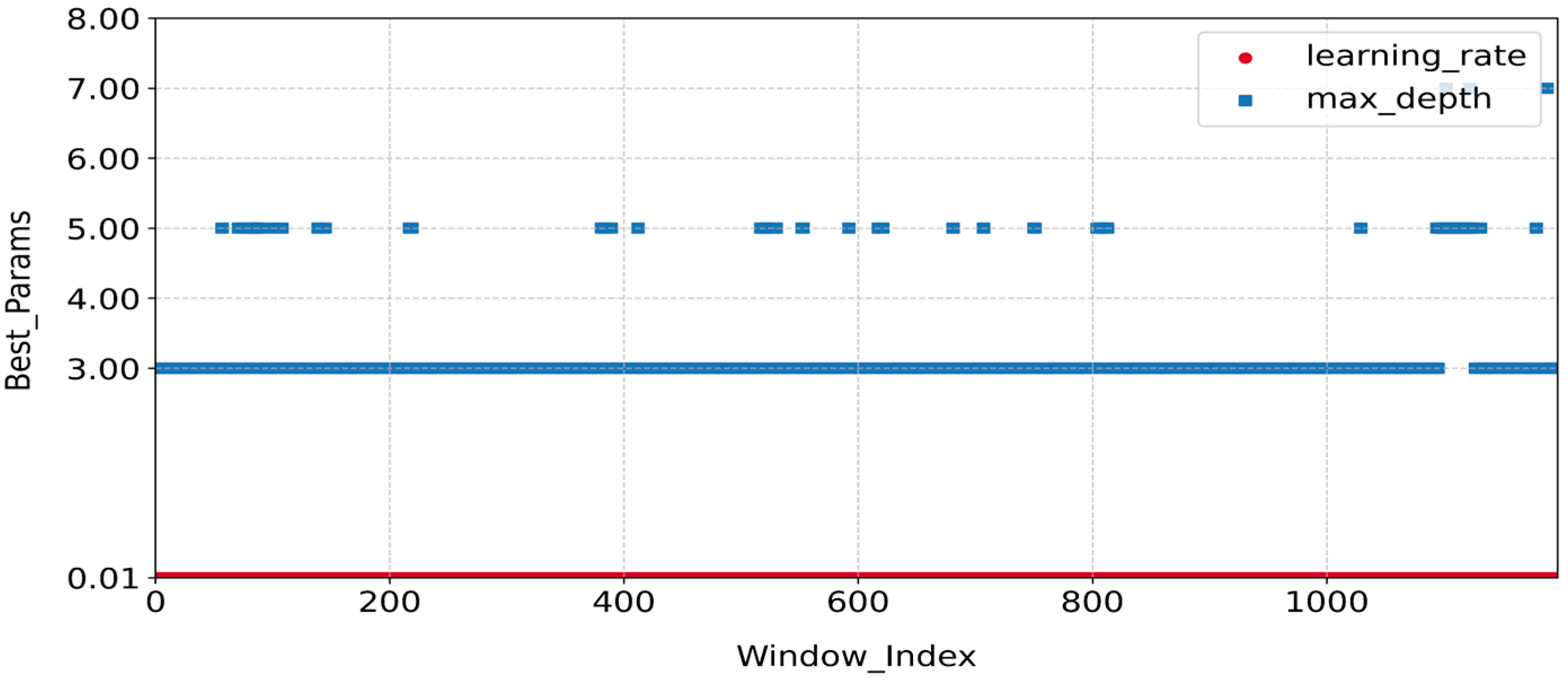
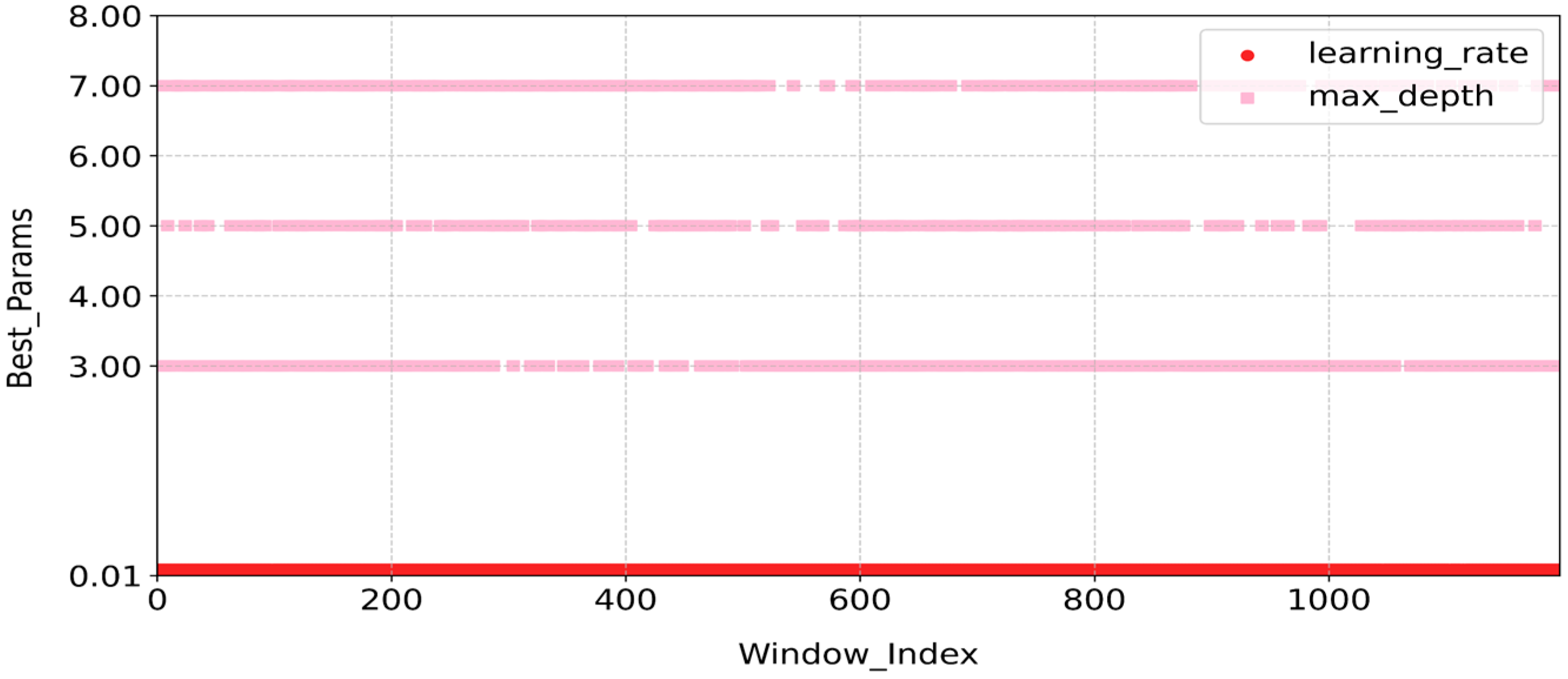
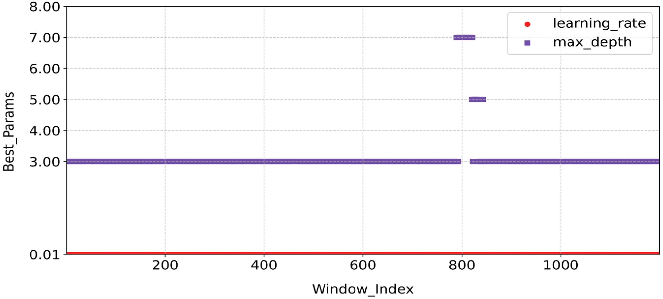
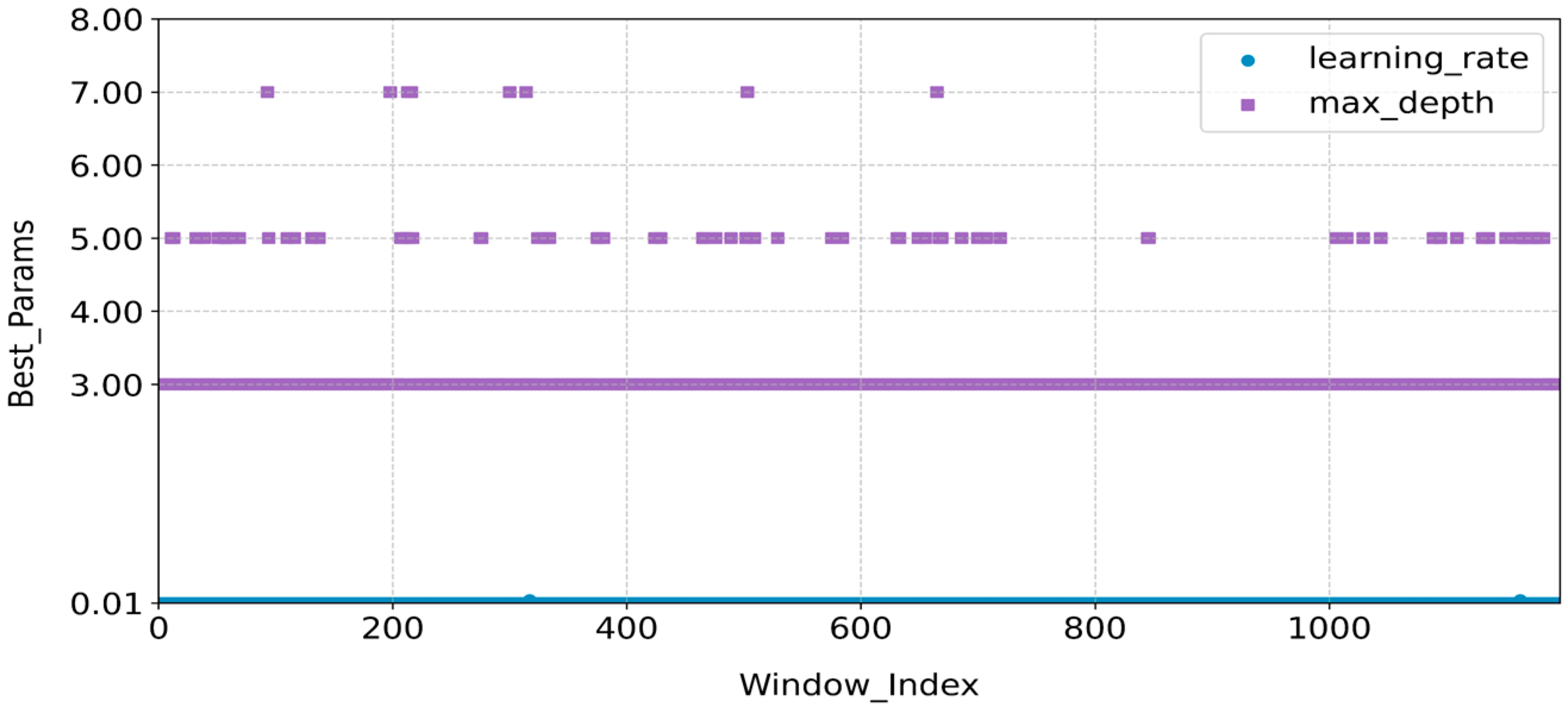
Figure A1.
Hyperparameter graph of GBR in univariate system.
Figure A1.
Hyperparameter graph of GBR in univariate system.
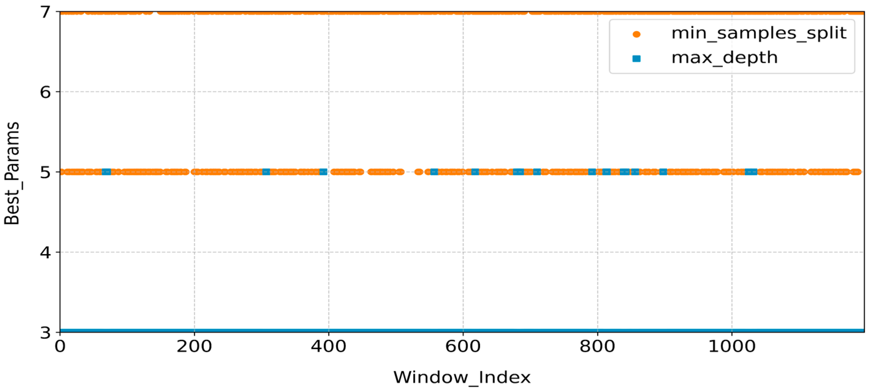
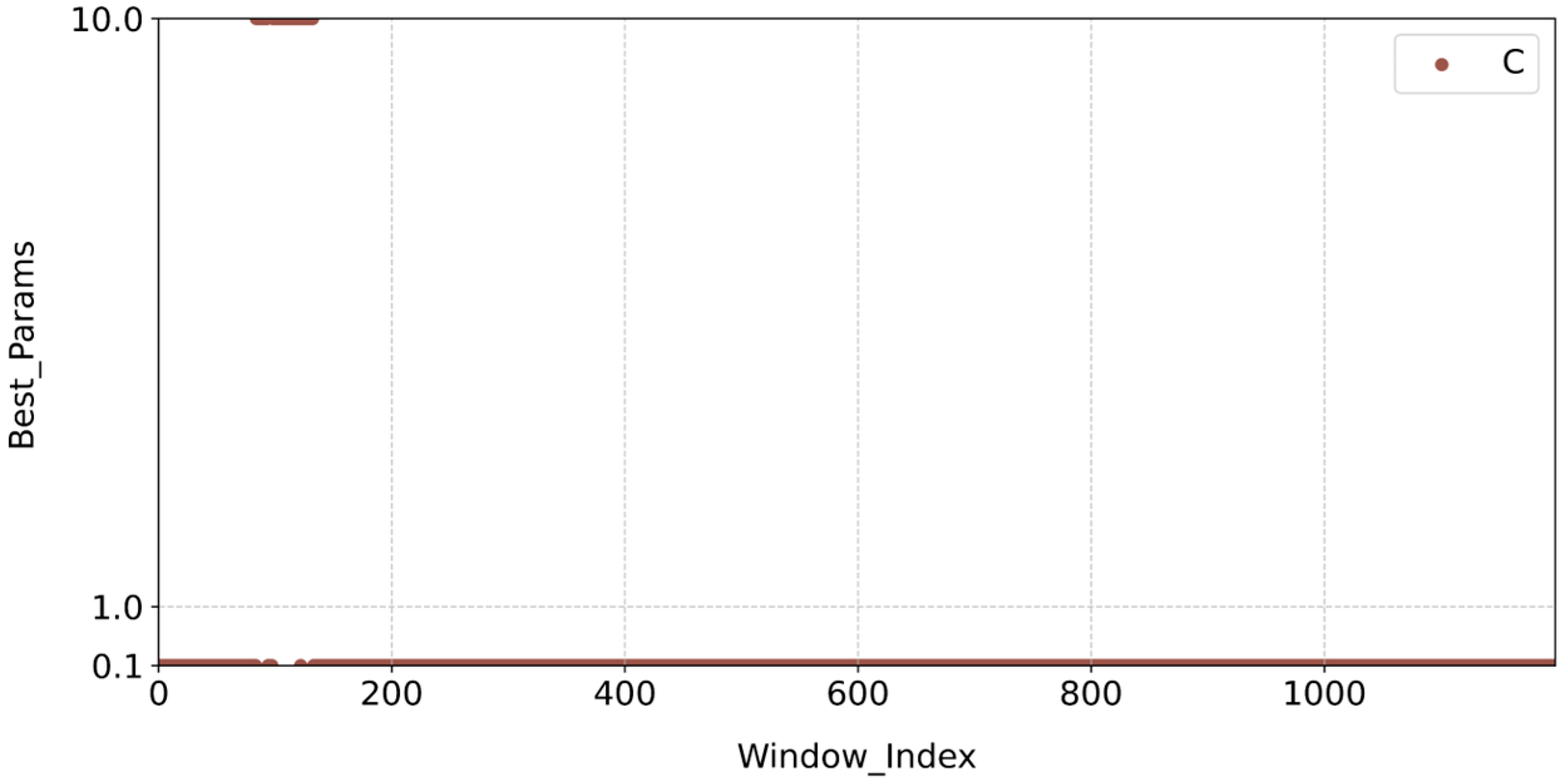
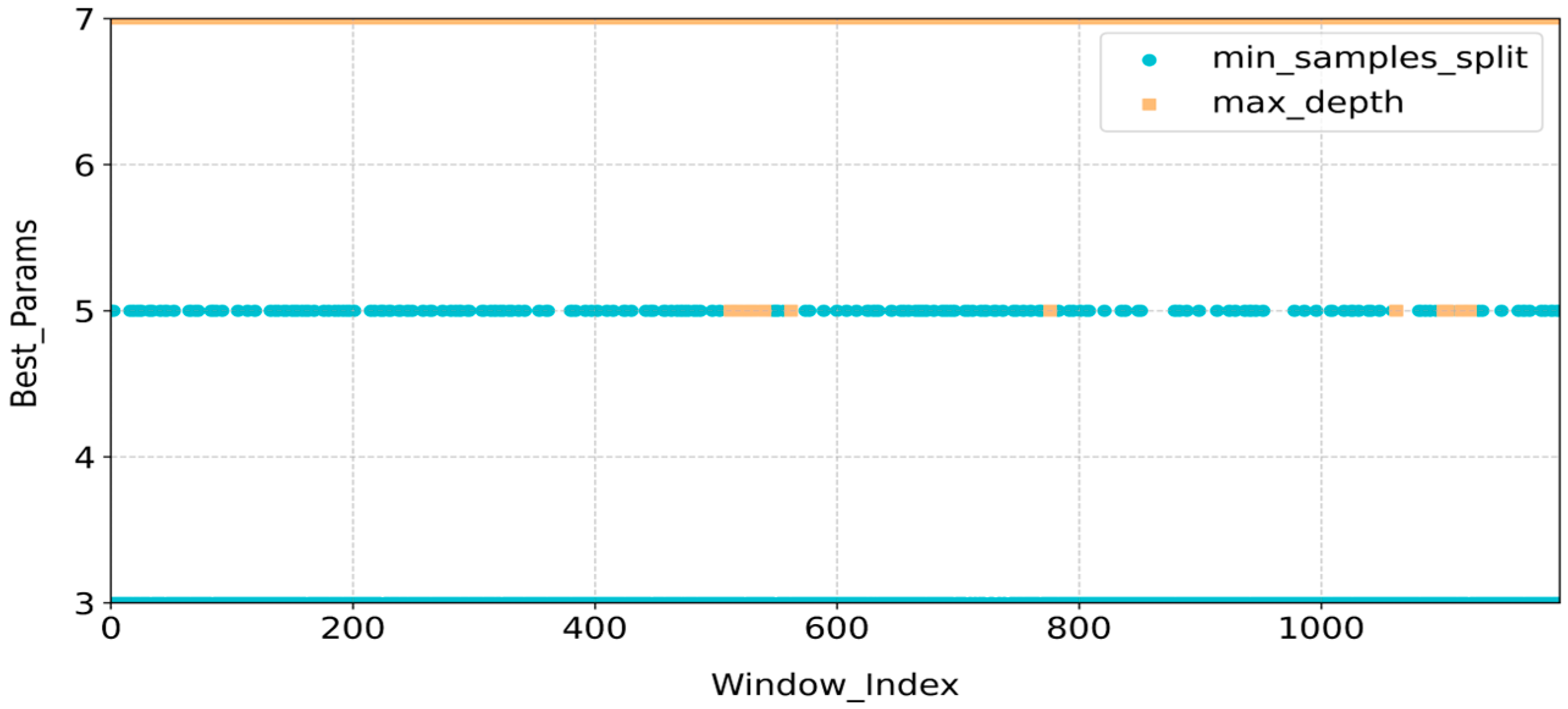
Figure A2.
Hyperparameter graph of RF in univariate system.
Figure A2.
Hyperparameter graph of RF in univariate system.
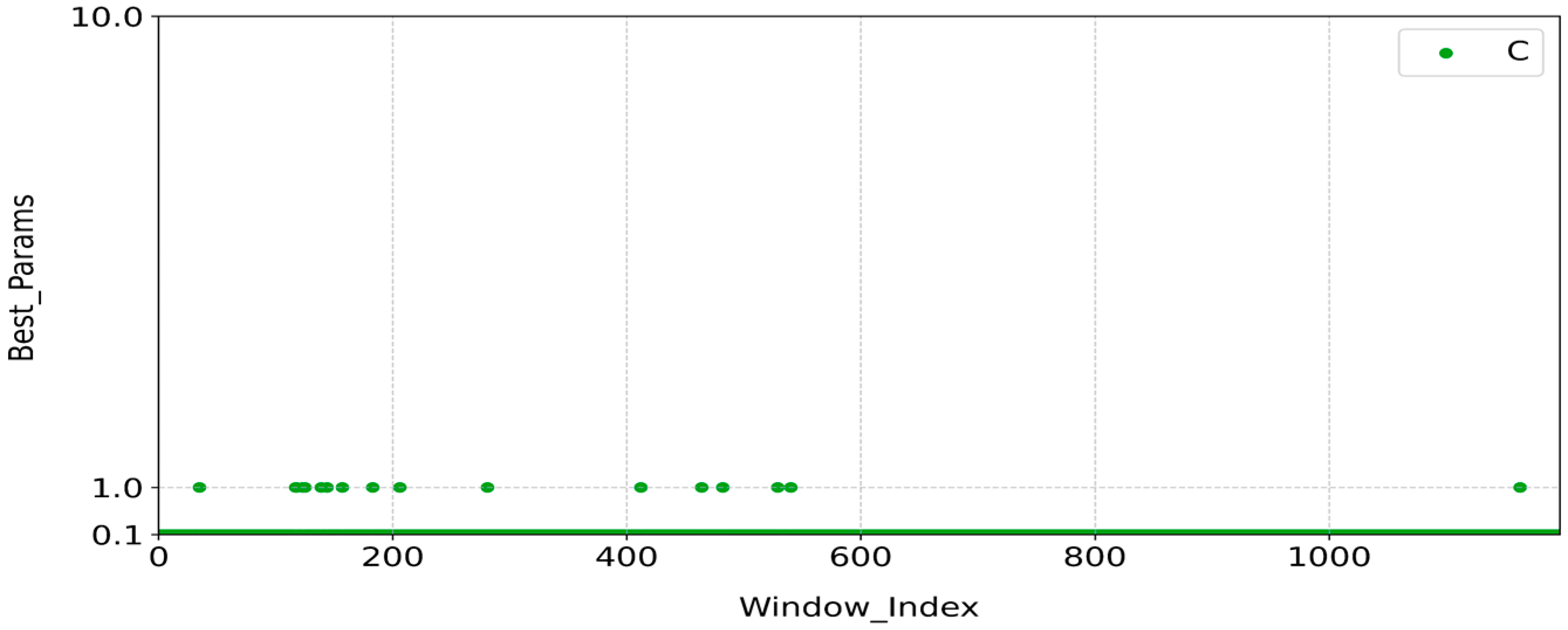
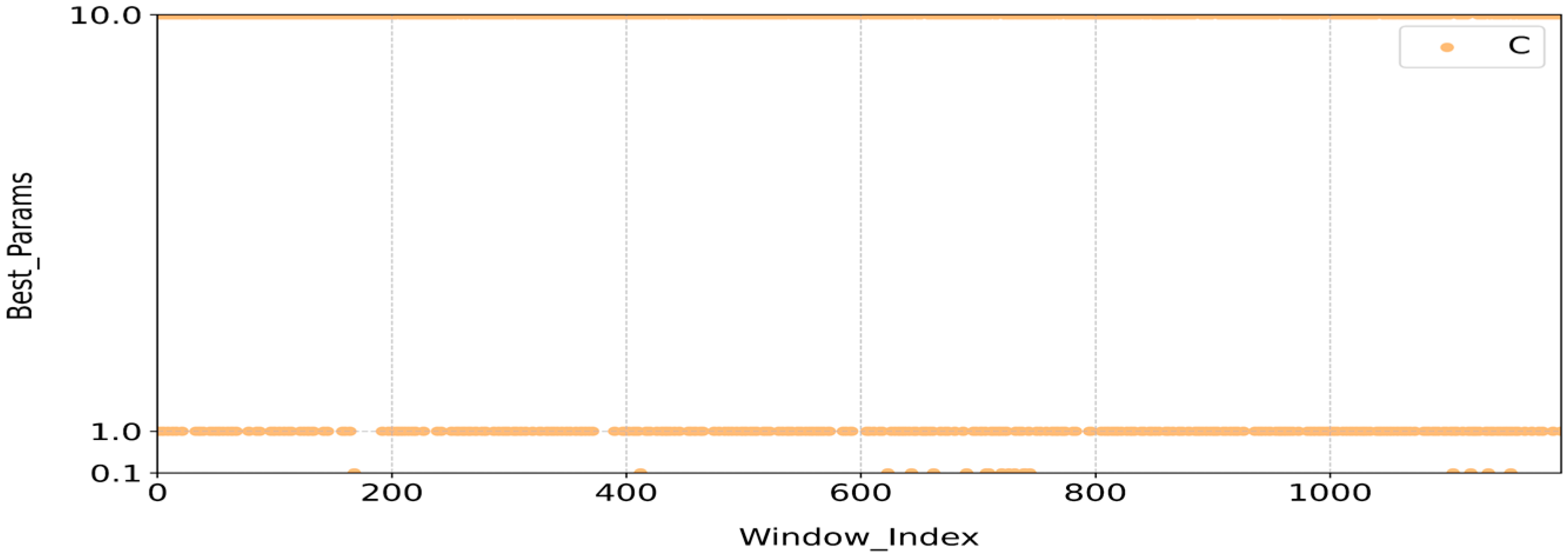
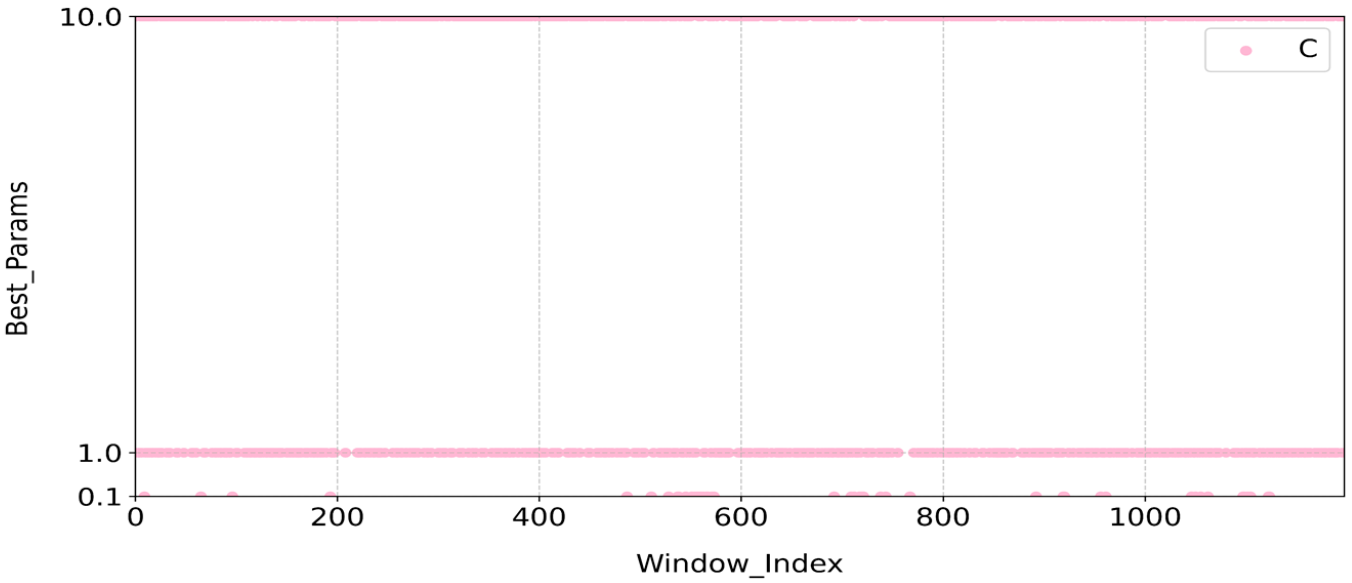
Figure A3.
Hyperparameter graph of SVR in univariate system.
Figure A3.
Hyperparameter graph of SVR in univariate system.
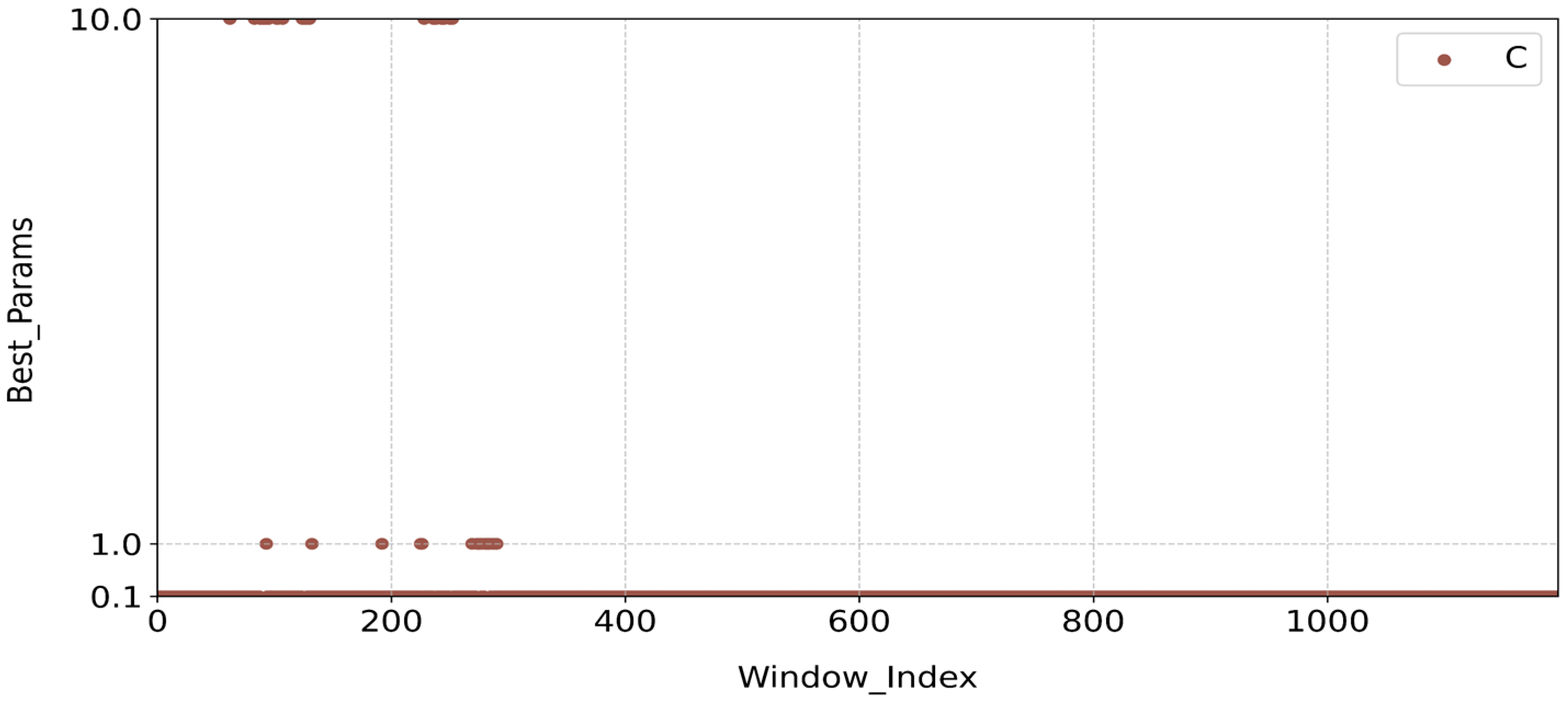
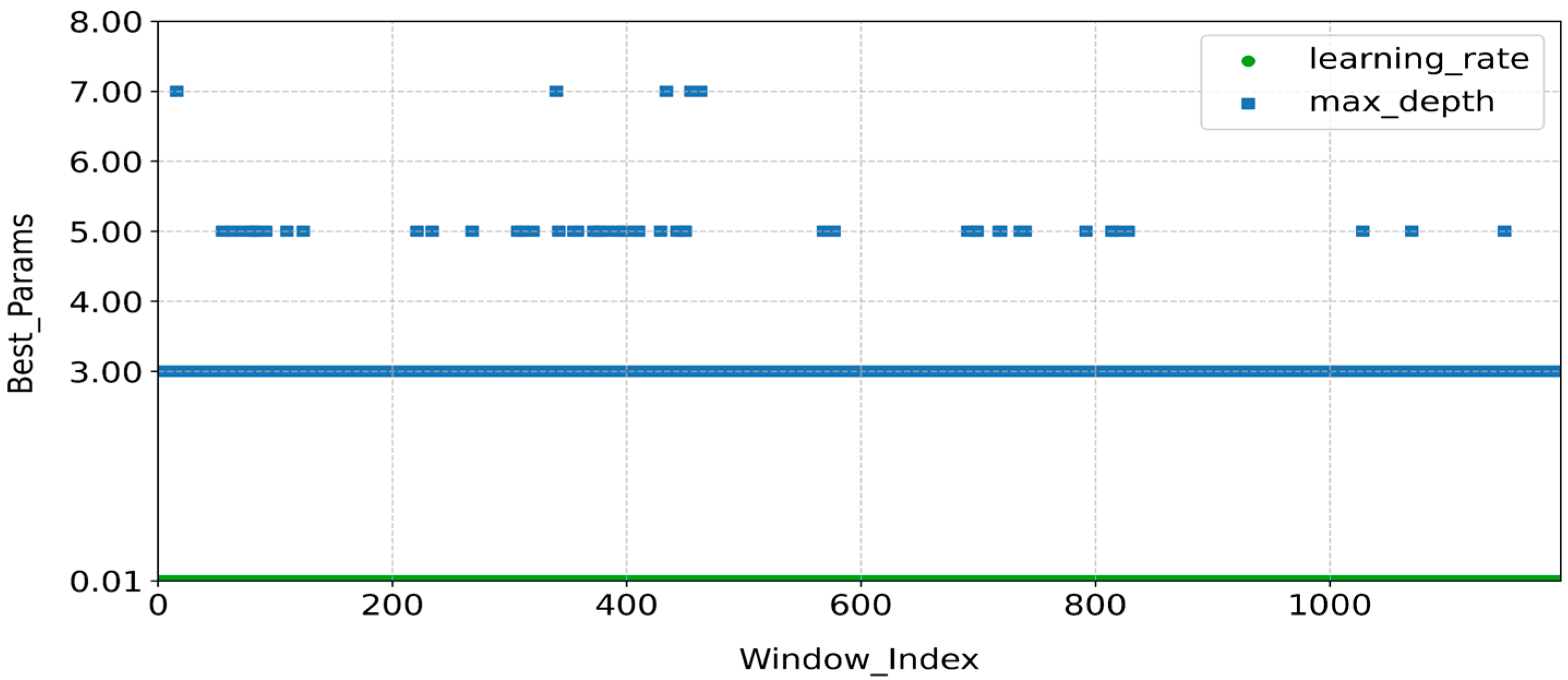
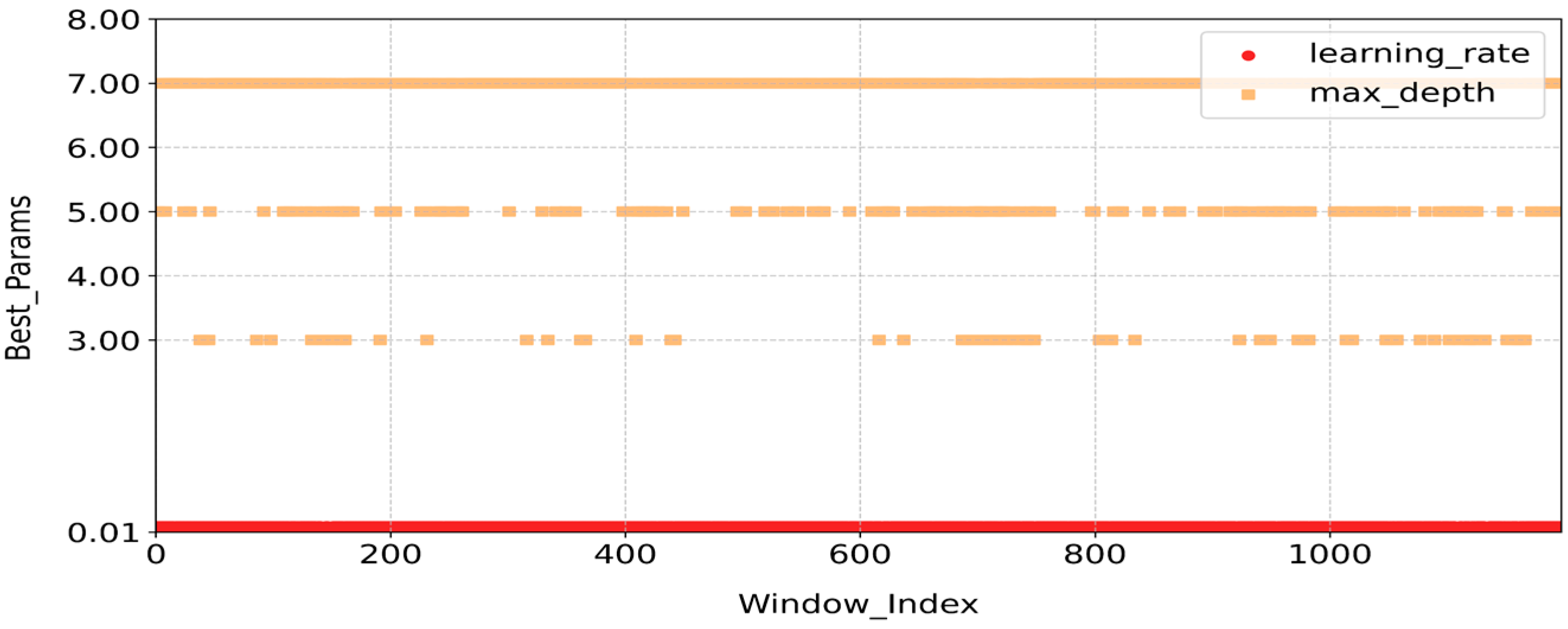
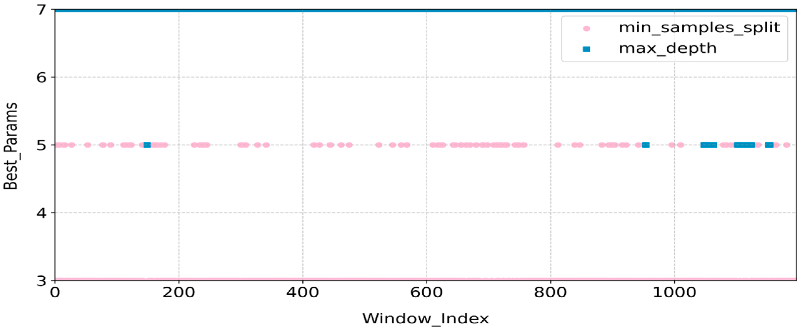
Figure A4.
Hyperparameter graph of XGB in univariate system.
Figure A4.
Hyperparameter graph of XGB in univariate system.
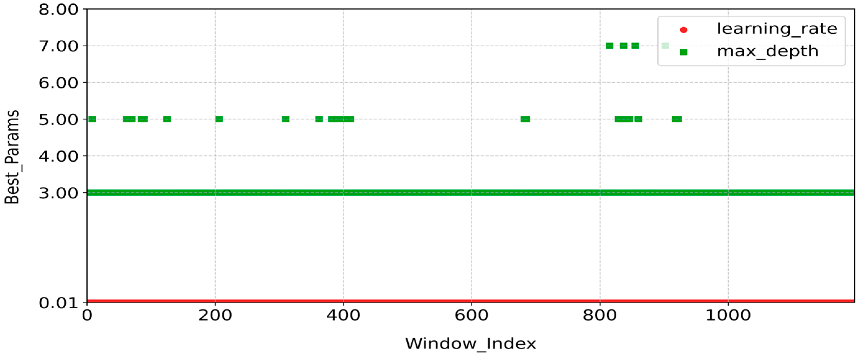
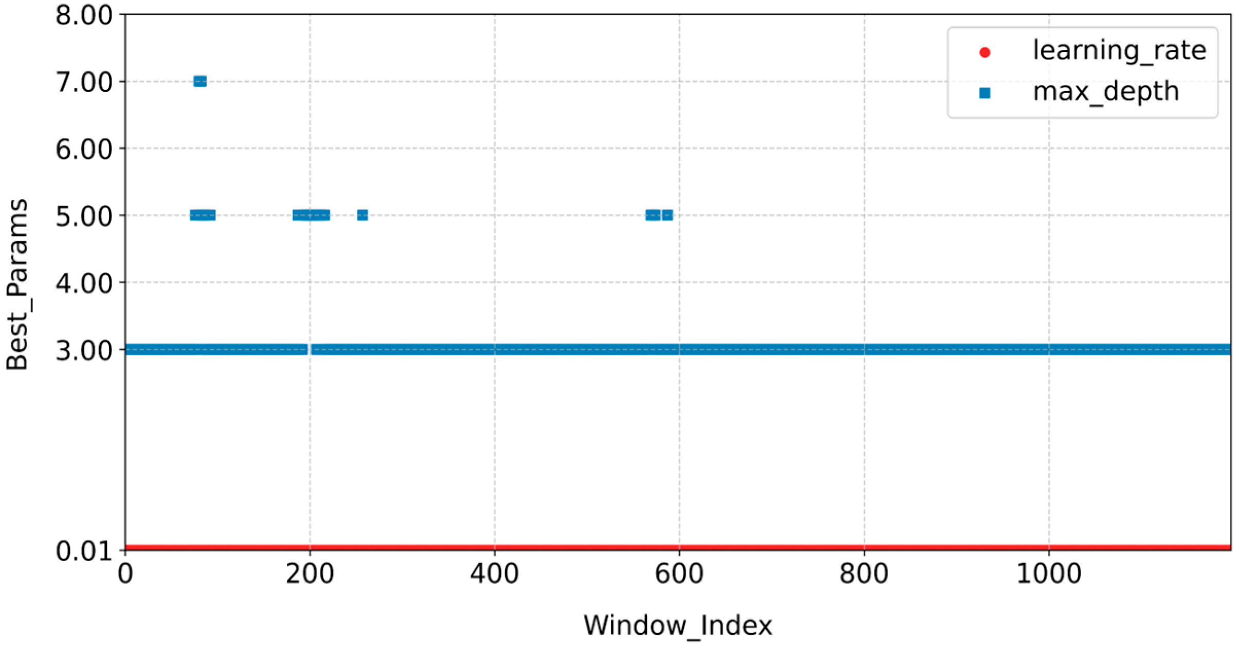
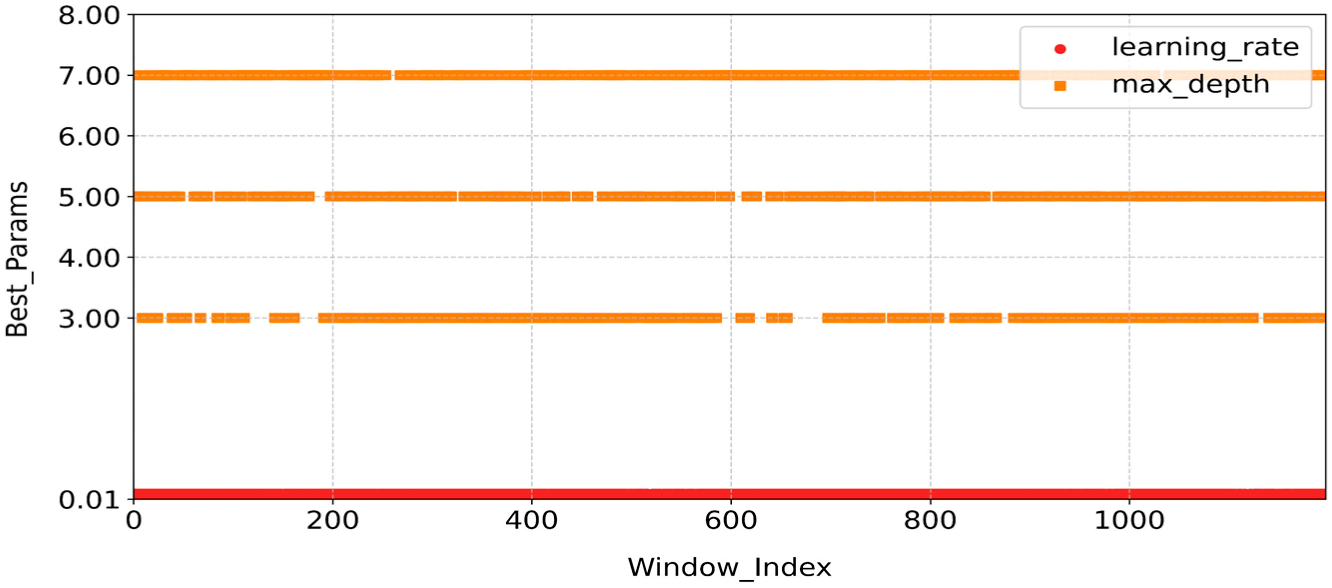
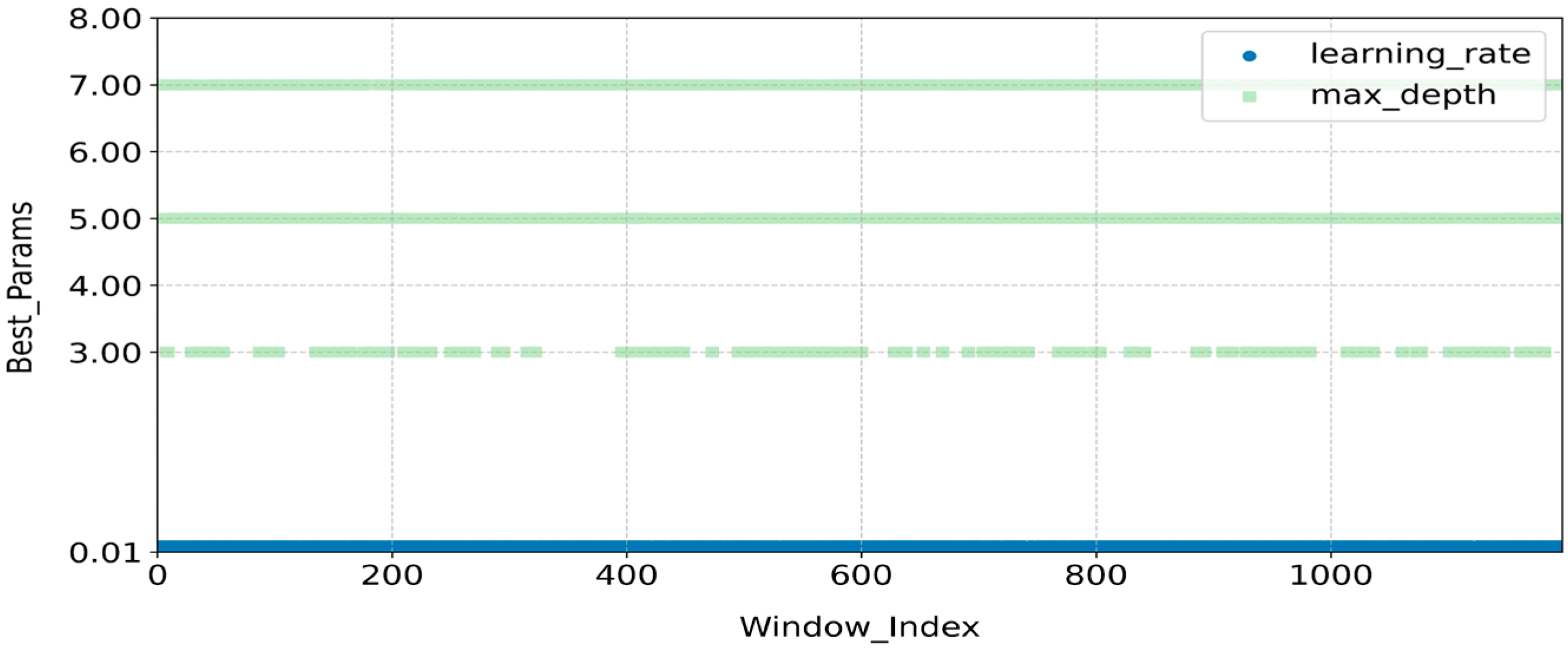
Figure A5.
Hyperparameter graph of GBR in multivariate system.
Figure A5.
Hyperparameter graph of GBR in multivariate system.
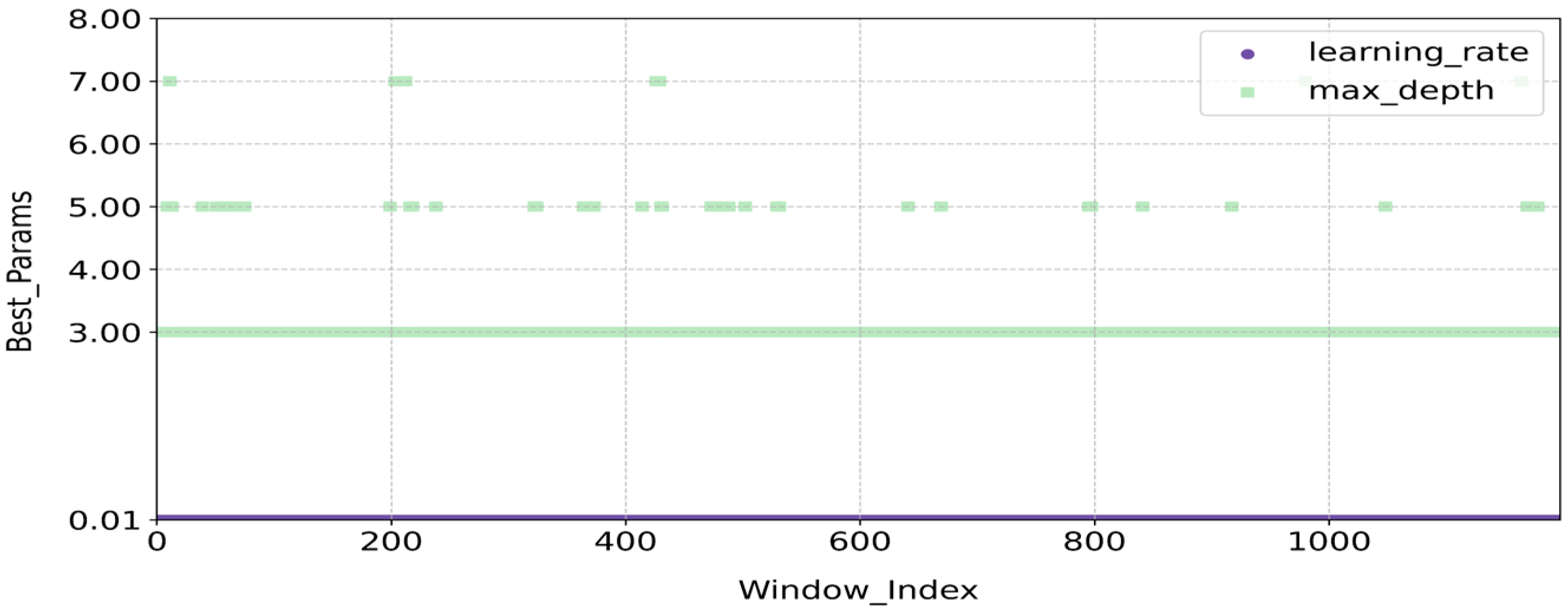
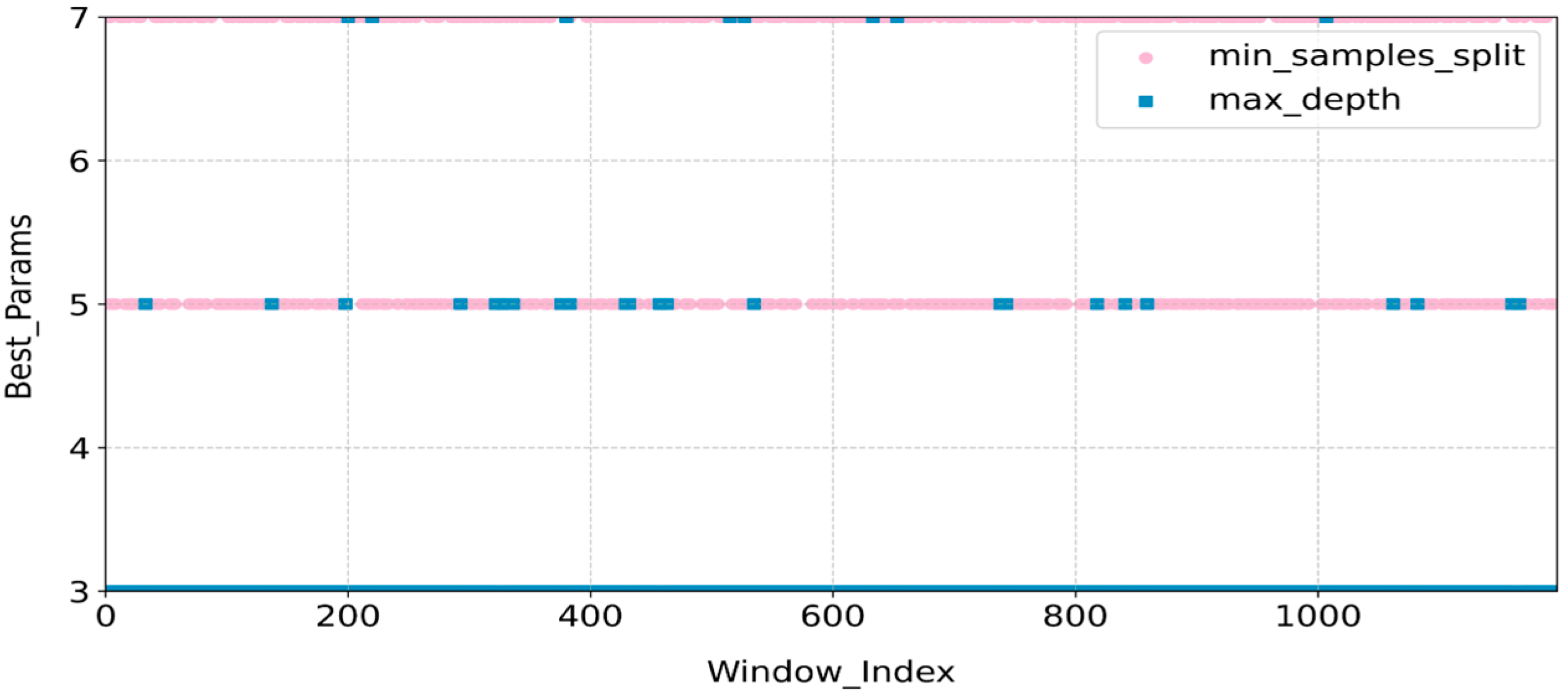
Figure A6.
Hyperparameter graph of RF in multivariate system.
Figure A6.
Hyperparameter graph of RF in multivariate system.
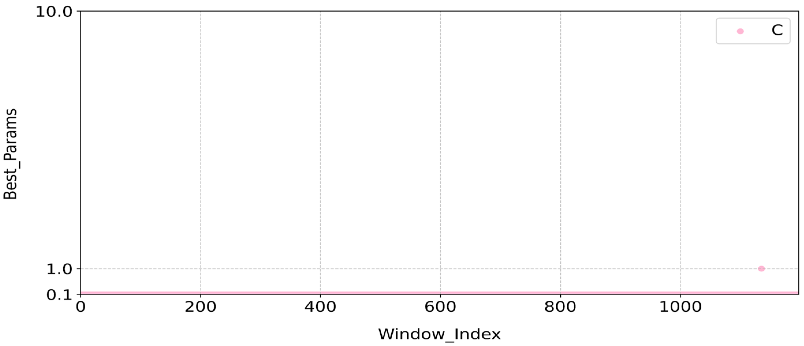
Figure A7.
Hyperparameter graph of SVR in multivariate system.
Figure A7.
Hyperparameter graph of SVR in multivariate system.
Figure A8.
Hyperparameter graph of XGB in multivariate system.
Figure A8.
Hyperparameter graph of XGB in multivariate system.
Figure A9.
Hyperparameter diagram of the high-frequency component of GBR in the “Sliding EMD” system.
Figure A9.
Hyperparameter diagram of the high-frequency component of GBR in the “Sliding EMD” system.
Figure A10.
Hyperparameter diagram of the high-frequency component of RF in the “Sliding EMD” system.
Figure A10.
Hyperparameter diagram of the high-frequency component of RF in the “Sliding EMD” system.
Figure A11.
Hyperparameter diagram of the high-frequency component of SVR in the “Sliding EMD” system.
Figure A11.
Hyperparameter diagram of the high-frequency component of SVR in the “Sliding EMD” system.
Figure A12.
Hyperparameter diagram of the high-frequency component of XGB in the “Sliding EMD” system.
Figure A12.
Hyperparameter diagram of the high-frequency component of XGB in the “Sliding EMD” system.
Figure A13.
Hyperparameter diagram of the low-frequency component of GBR in the “Sliding EMD” system.
Figure A13.
Hyperparameter diagram of the low-frequency component of GBR in the “Sliding EMD” system.
Figure A14.
Hyperparameter diagram of the low-frequency component of RF in the “Sliding EMD” system.
Figure A14.
Hyperparameter diagram of the low-frequency component of RF in the “Sliding EMD” system.
Figure A15.
Hyperparameter diagram of the low-frequency component of SVR in the “Sliding EMD” system.
Figure A15.
Hyperparameter diagram of the low-frequency component of SVR in the “Sliding EMD” system.
Figure A16.
Hyperparameter diagram of the low-frequency component of XGB in the “Sliding EMD” system.
Figure A16.
Hyperparameter diagram of the low-frequency component of XGB in the “Sliding EMD” system.
Figure A17.
The hyperparameter graph of the GBR high-frequency components of the “Sliding EMD–Multi Variables” system.
Figure A17.
The hyperparameter graph of the GBR high-frequency components of the “Sliding EMD–Multi Variables” system.
Figure A18.
The hyperparameter graph of the RF high-frequency components of the “Sliding EMD–Multi Variables” system.
Figure A18.
The hyperparameter graph of the RF high-frequency components of the “Sliding EMD–Multi Variables” system.
Figure A19.
The hyperparameter graph of the SVR high-frequency components of the “Sliding EMD–Multi Variables” system.
Figure A19.
The hyperparameter graph of the SVR high-frequency components of the “Sliding EMD–Multi Variables” system.
Figure A20.
The hyperparameter graph of the XGB high-frequency components of the “Sliding EMD–Multi Variables” system.
Figure A20.
The hyperparameter graph of the XGB high-frequency components of the “Sliding EMD–Multi Variables” system.
Figure A21.
The hyperparameter graph of the GBR low-frequency components of the “Sliding EMD–Multi Variables” system.
Figure A21.
The hyperparameter graph of the GBR low-frequency components of the “Sliding EMD–Multi Variables” system.
Figure A22.
The hyperparameter graph of the RF low-frequency components of the “Sliding EMD–Multi Variables” system.
Figure A22.
The hyperparameter graph of the RF low-frequency components of the “Sliding EMD–Multi Variables” system.
Figure A23.
The hyperparameter graph of the SVR low-frequency components of the “Sliding EMD–Multi Variables” system.
Figure A23.
The hyperparameter graph of the SVR low-frequency components of the “Sliding EMD–Multi Variables” system.
Figure A24.
The hyperparameter graph of the XGB low-frequency components of the “Sliding EMD–Multi Variables” system.
Figure A24.
The hyperparameter graph of the XGB low-frequency components of the “Sliding EMD–Multi Variables” system.
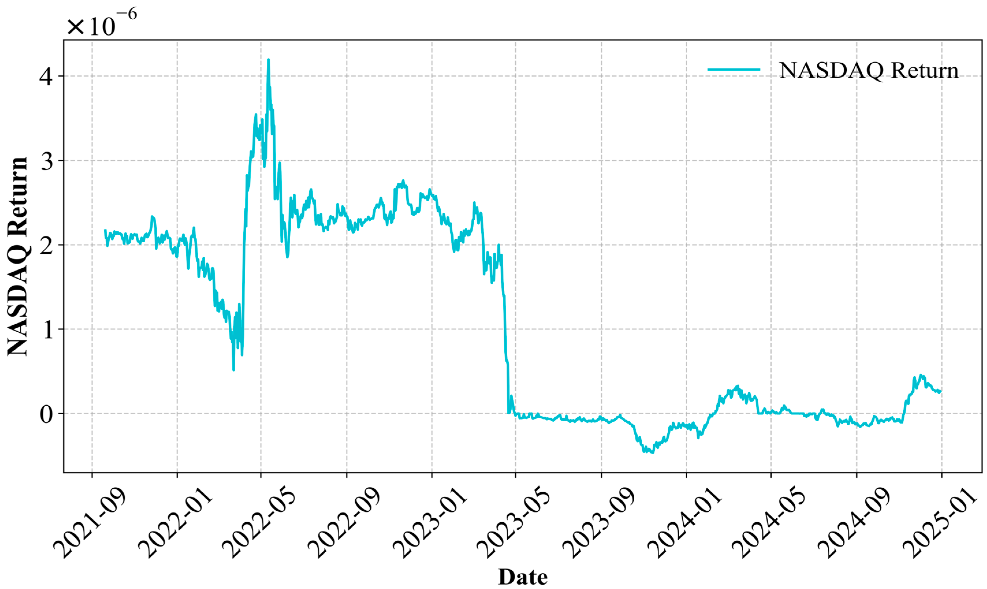
Figure A25.
Multivariate system prediction result graph.
Figure A25.
Multivariate system prediction result graph.
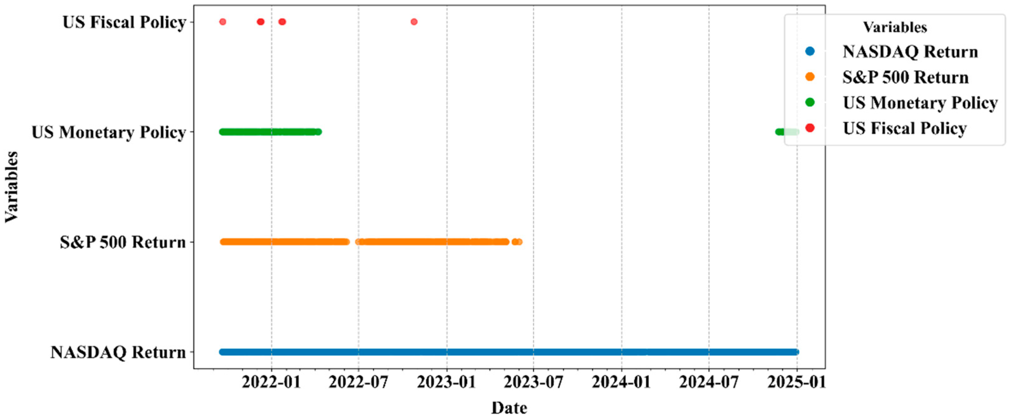
Figure A26.
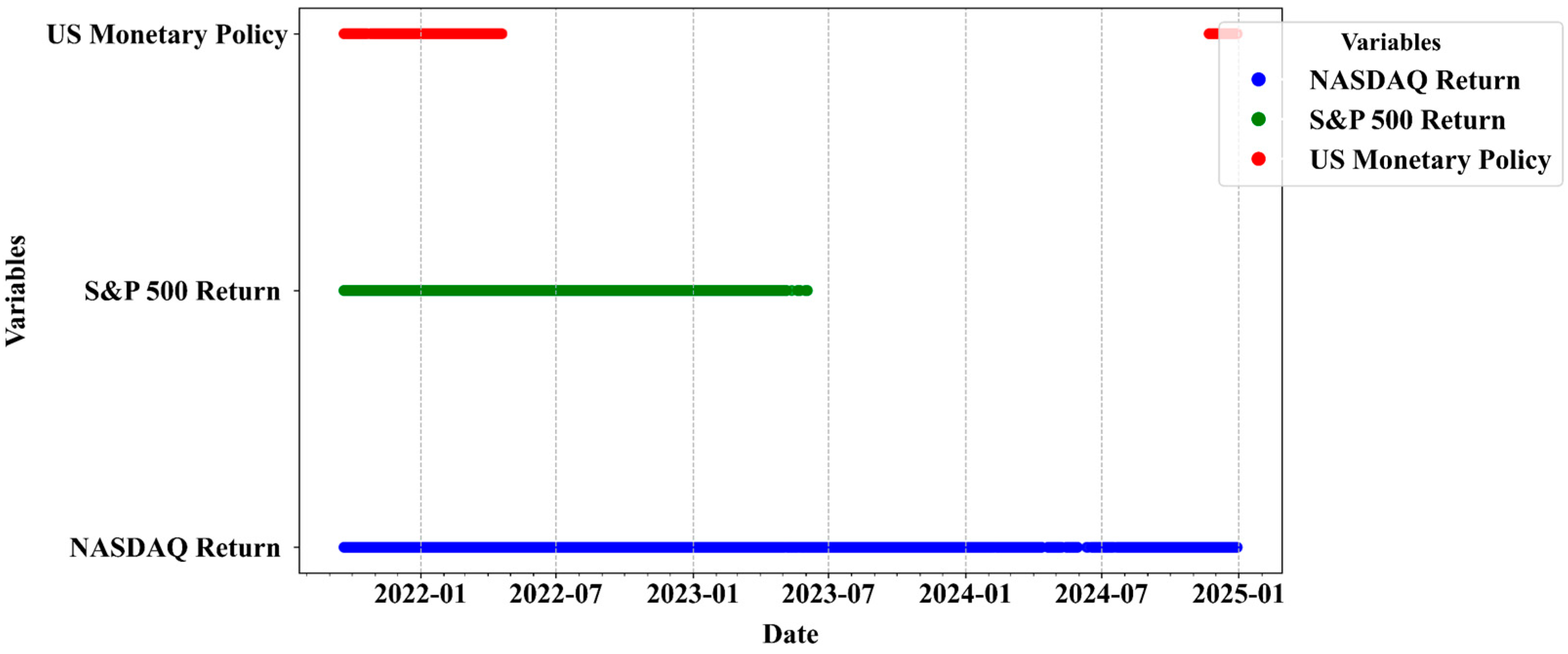
The Lasso selection relationship coefficient graph of the multivariable system Nasdaq.
Figure A26.
The Lasso selection relationship coefficient graph of the multivariable system Nasdaq.
Figure A27.
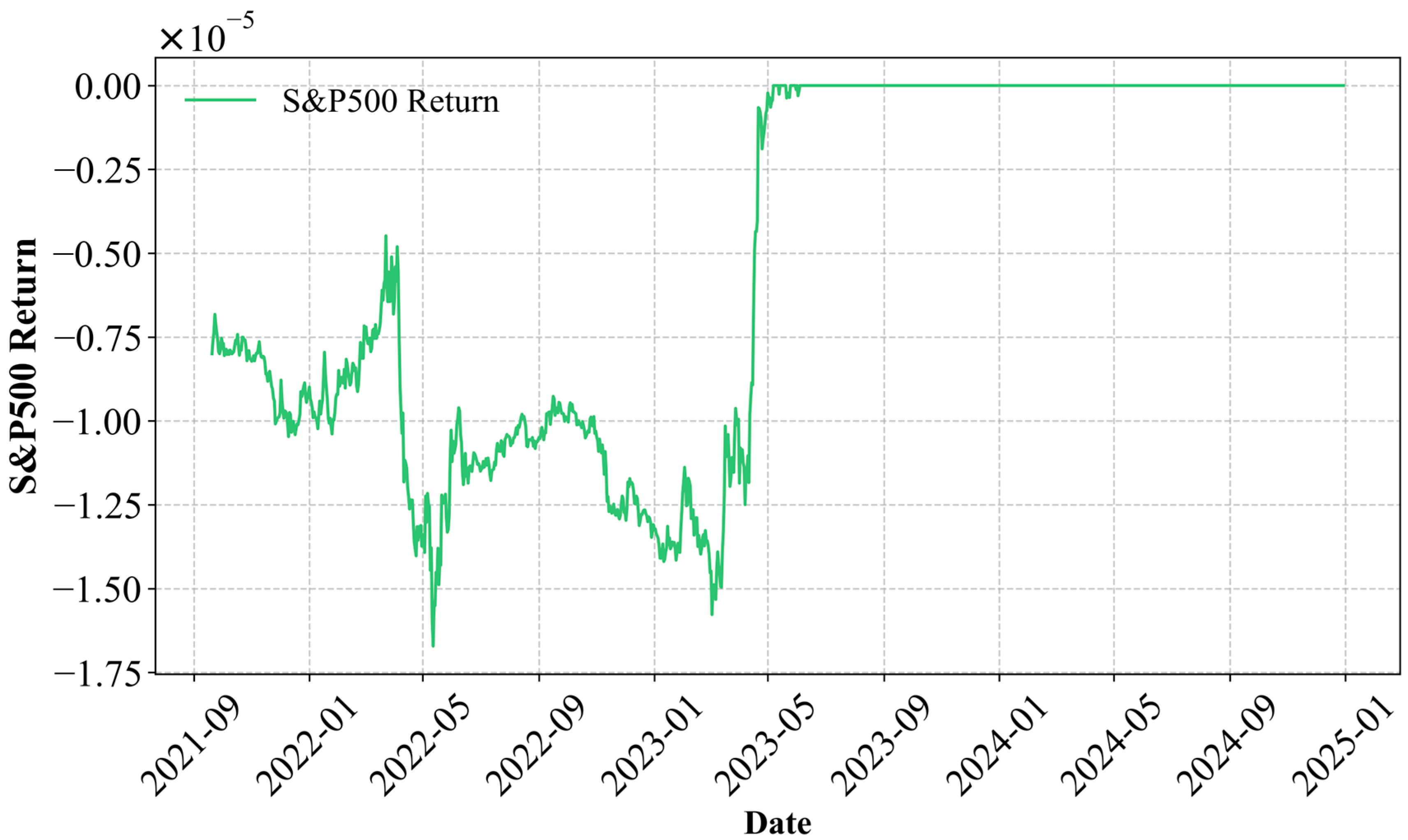
The Lasso selection relationship coefficient graph of the multivariable system Sp500.
Figure A27.
The Lasso selection relationship coefficient graph of the multivariable system Sp500.
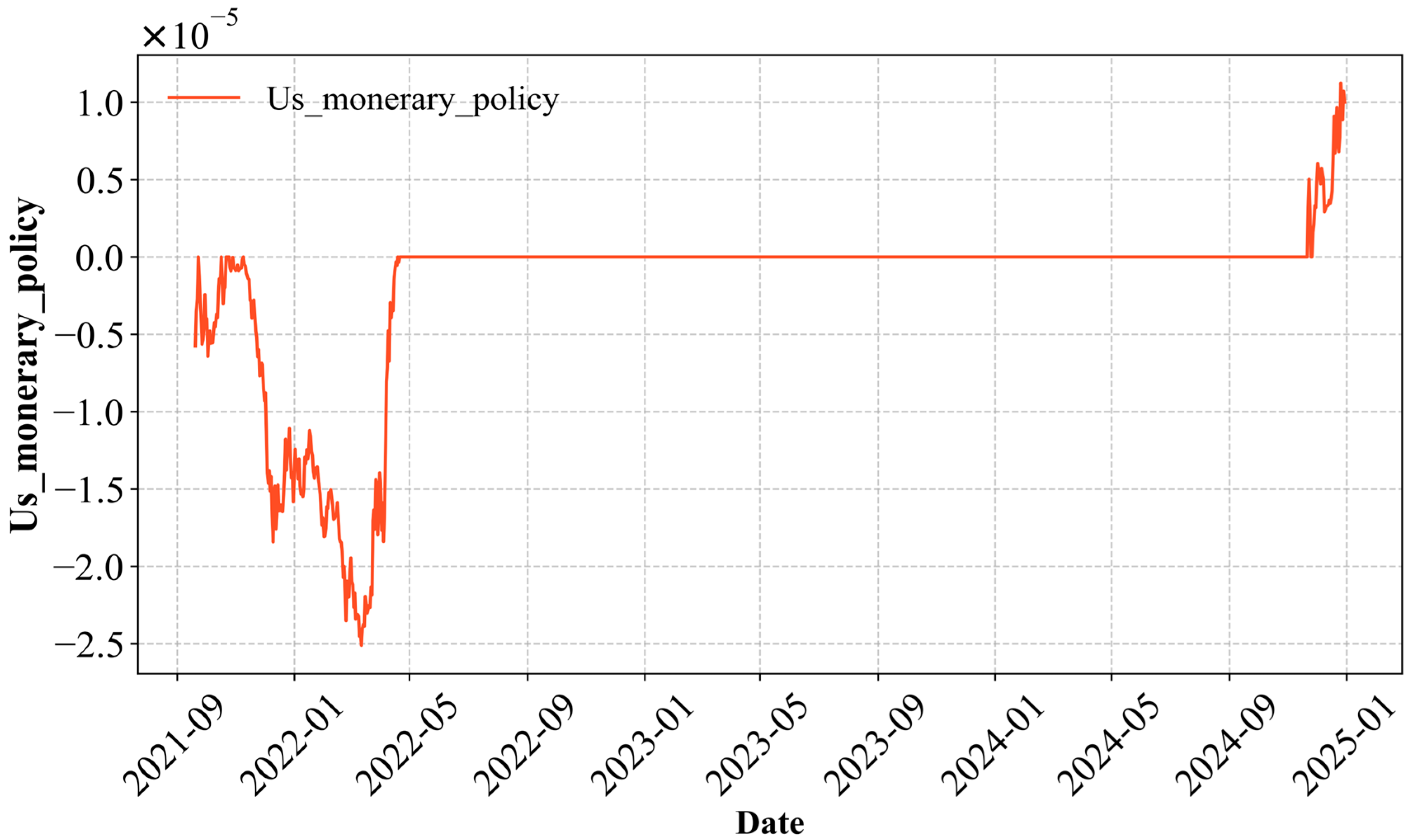
Figure A28.
The Lasso choice relationship coefficient diagram of Us monetary policy in a multivariate system.
Figure A28.
The Lasso choice relationship coefficient diagram of Us monetary policy in a multivariate system.
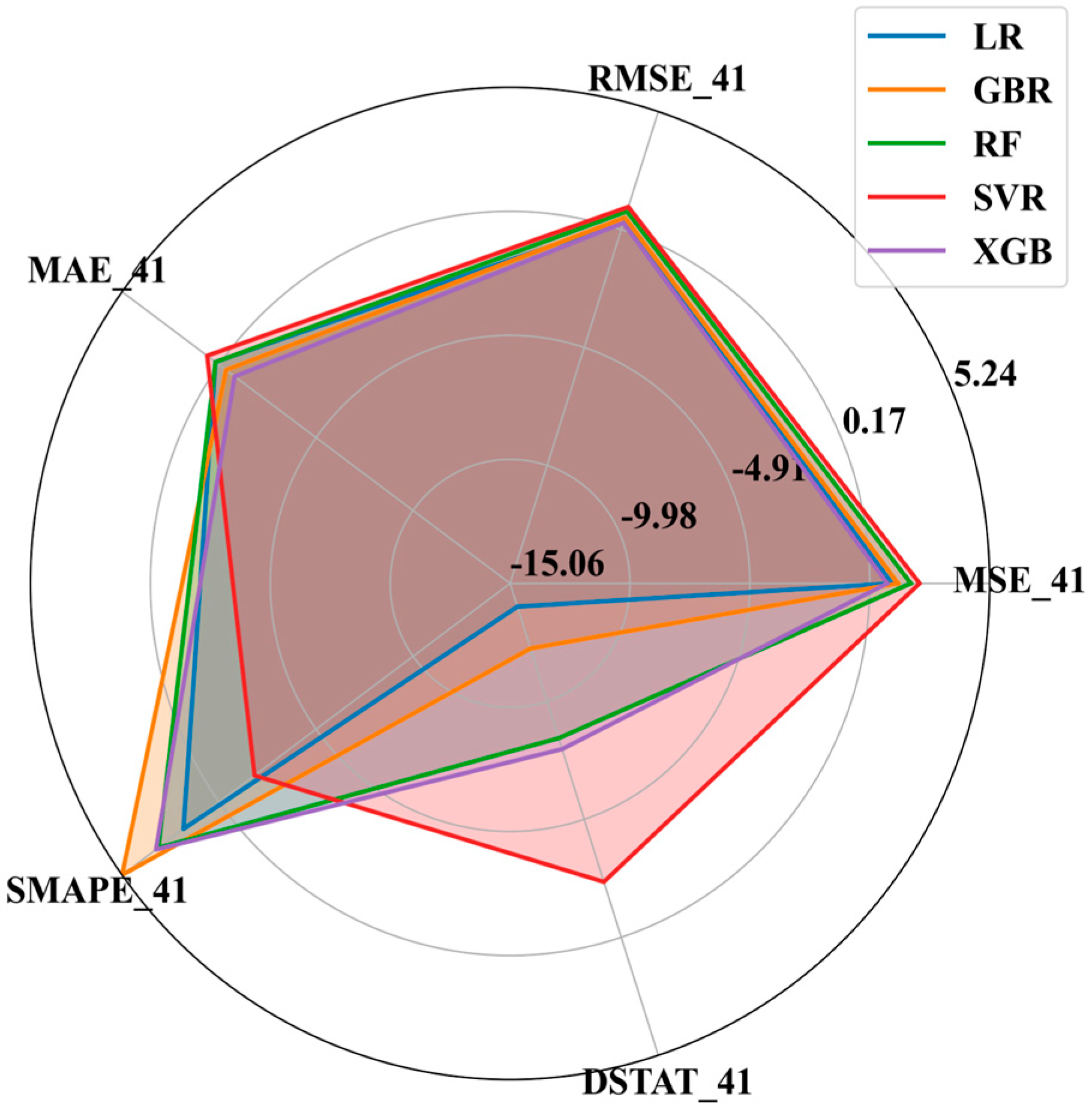
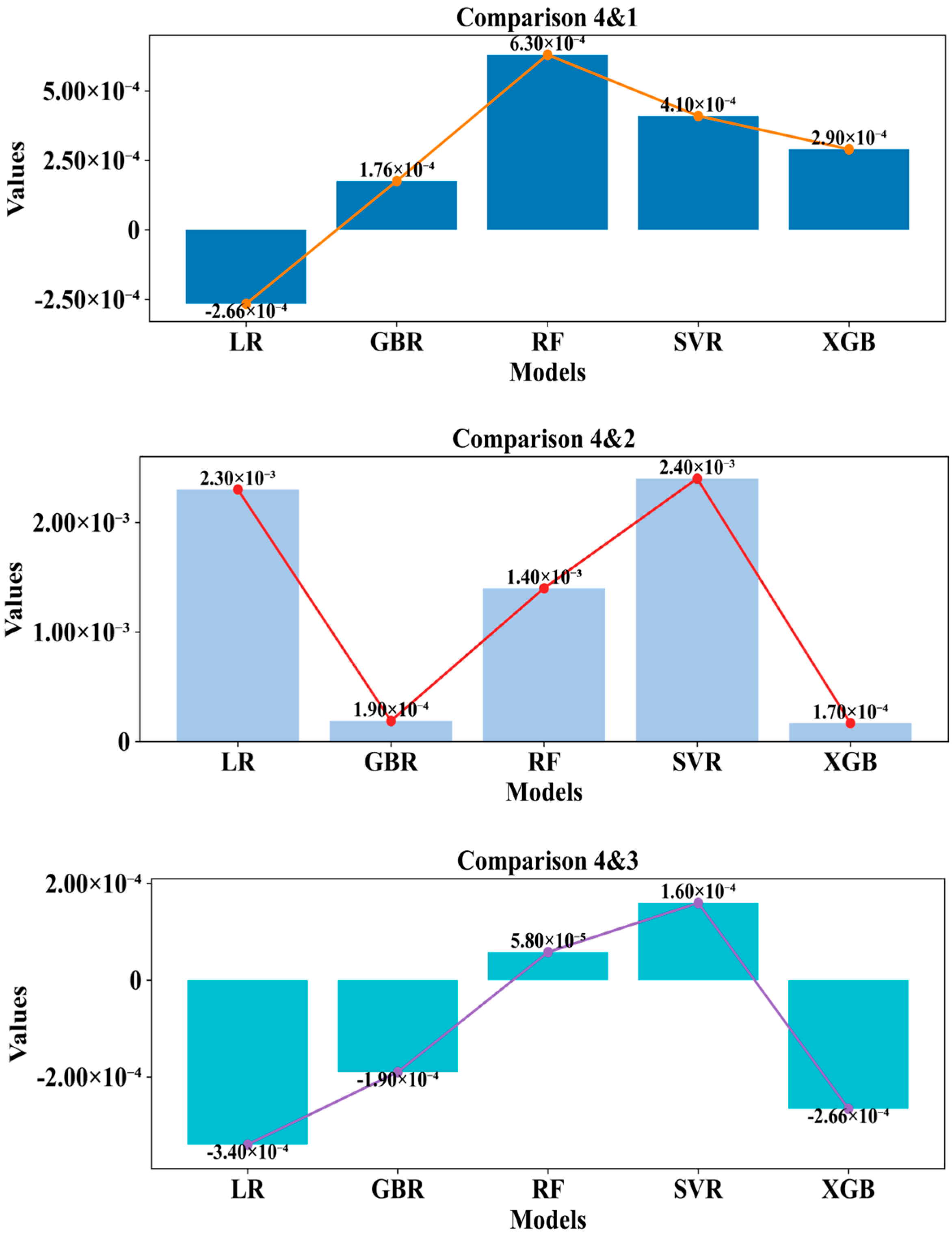
Figure A29.
Comparison of prediction accuracy between the “Sliding EMD-Multi Variables” system and the Multivariate Prediction System.
Figure A29.
Comparison of prediction accuracy between the “Sliding EMD-Multi Variables” system and the Multivariate Prediction System.
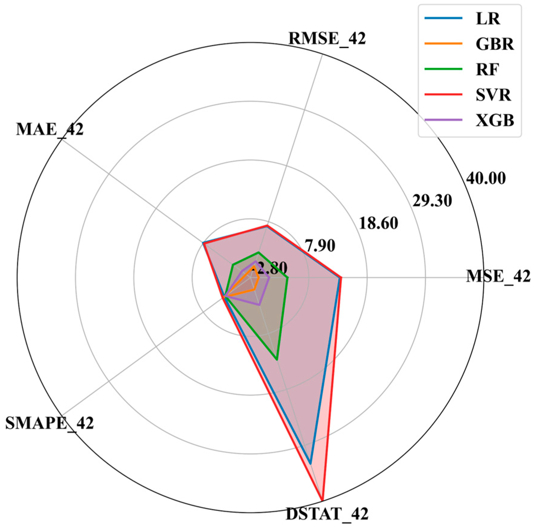
Figure A30.
Comparison of prediction accuracy between the “Sliding EMD-Multi Variables” system and the Univariate Prediction System.
Figure A30.
Comparison of prediction accuracy between the “Sliding EMD-Multi Variables” system and the Univariate Prediction System.
Table A1.
Error index table of univariate system results.
Table A1.
Error index table of univariate system results.
| | LR | GBR | RF | SVR | XGB |
|---|
| MSE_1 | 3.54 × 10⁻⁴ | 3.62 × 10⁻⁴ | 3.63 × 10⁻⁴ | 3.65 × 10⁻⁴ | 3.60 × 10⁻⁴ |
| RMSE_1 | 0.0188 | 0.0190 | 0.0190 | 0.0191 | 0.0190 |
| MAE_1 | 0.0134 | 0.0135 | 0.0135 | 0.0136 | 0.0134 |
| SMAPE_1 | 1.72 | 1.78 | 1.74 | 1.64 | 1.75 |
| DSTAT_1 | 0.510 | 0.489 | 0.504 | 0.503 | 0.493 |
Table A2.
MCS test result table of multivariate system.
Table A2.
MCS test result table of multivariate system.
| Index | Comparison_2&1 |
|---|
| |
|---|
| 1 | SVR_2 (0.000) | SVR_2 (0.000) |
| 2 | LR_2 (0.000) | LR_2 (0.003) |
| 3 | RF_2 (0.018) | RF_2 (0.159 *) |
| 4 | SVR_1 (0.061) | SVR_1 (0.269 **) |
| 5 | RF_1 (0.186 *) | RF_1 (0.377 **) |
| 6 | GBR_1 (0.288 **) | GBR_1 (0.448 **) |
| 7 | XGB_1 (0.377 **) | XGB_1 (0.530 **) |
| 8 | XGB_2 (0.564 **) | XGB_2 (0.676 **) |
| 9 | LR_1 (0.866 **) | LR_1 (0.866 **) |
| 10 | GBR_2 (1.000 **) | GBR_2 (1.000 **) |
Table A3.
The result table of Maximum Drawdown Ratio of the “Sliding EMD” system.
Table A3.
The result table of Maximum Drawdown Ratio of the “Sliding EMD” system.
| Maximum Drawdown Ratio | Comparison_3&1 | Comparison_3&2 |
|---|
| LR | 0.165 | 0.629 |
| GBR | 0.199 | 0.366 |
| RF | 0.247 | 0.519 |
| SVR | 0.165 | 0.527 |
| XGB | 0.198 | 0.300 |
Table A4.
The result table of Sharpe Ratio of the “Sliding EMD” system.
Table A4.
The result table of Sharpe Ratio of the “Sliding EMD” system.
| Sharpe Ratio | Comparison_3&1 | Comparison_3&2 |
|---|
| LR | 0.0371 | 3.77 |
| GBR | 0.297 | 0.314 |
| RF | 0.687 | 1.42 |
| SVR | 0.239 | 2.54 |
| XGB | 0.533 | 0.413 |
Table A5.
The Sortino Ratio result table of the “Sliding EMD” system.
Table A5.
The Sortino Ratio result table of the “Sliding EMD” system.
| Sortino Ratio | Comparison_3&1 | Comparison_3&2 |
|---|
| LR | 0.0905 | 8.69 |
| GBR | 0.764 | 0.857 |
| RF | 1.79 | 3.91 |
| SVR | 0.665 | 6.71 |
| XGB | 1.44 | 1.17 |
Table A6.
The Calmar Ratio result table of the “Sliding EMD” system.
Table A6.
The Calmar Ratio result table of the “Sliding EMD” system.
| Calmar Ratio | Comparison_3&1 | Comparison_3&2 |
|---|
| LR | 0.0579 | 0.551 |
| GBR | 0.128 | 0.0573 |
| RF | 0.228 | 0.330 |
| SVR | 0.109 | 0.475 |
| XGB | 0.230 | 0.138 |
Table A7.
The result table of the Maximum Drawdown Ratio of the “Sliding EMD-Multi Variables” system.
Table A7.
The result table of the Maximum Drawdown Ratio of the “Sliding EMD-Multi Variables” system.
| Maximum Drawdown Ratio | Comparison_4&1 | Comparison_4&2 | Comparison_4&3 |
|---|
| LR | −0.0173 | 0.447 | −0.182 |
| GBR | 0.0961 | 0.264 | −0.102 |
| RF | 0.277 | 0.549 | 0.0299 |
| SVR | 0.293 | 0.655 | 0.128 |
| XGB | 0.180 | 0.281 | −0.0181 |
Table A8.
The result table of Sharpe Ratio of the “Sliding EMD-Multi Variables” system.
Table A8.
The result table of Sharpe Ratio of the “Sliding EMD-Multi Variables” system.
| Sharpe Ratio | Comparison_4&1 | Comparison_4&2 | Comparison_4&3 |
|---|
| LR | −0.385 | 3.34 | −0.422 |
| GBR | −0.0500 | 0.0671 | −0.247 |
| RF | 0.760 | 1.50 | 0.0732 |
| SVR | 0.470 | 2.78 | 0.231 |
| XGB | −0.224 | 0.0562 | −0.357 |
Table A9.
The Sortino Ratio result table of the “Sliding EMD-Multi Variables” system.
Table A9.
The Sortino Ratio result table of the “Sliding EMD-Multi Variables” system.
| Sortino Ratio | Comparison_4&1 | Comparison_4&2 | Comparison_4&3 |
|---|
| LR | −1.12 | 7.48 | −1.21 |
| GBR | 0.0465 | 0.139 | −0.718 |
| RF | 2.04 | 4.15 | 0.250 |
| SVR | 1.39 | 7.44 | 0.726 |
| XGB | 0.445 | 0.171 | −0.992 |
Table A10.
The Calmar Ratio result table of the “Sliding EMD-Multi Variables” system.
Table A10.
The Calmar Ratio result table of the “Sliding EMD-Multi Variables” system.
| Calmar Ratio | Comparison_4&1 | Comparison_4&2 | Comparison_4&3 |
|---|
| LR | −0.144 | 0.349 | −0.202 |
| GBR | 0.0412 | −0.0296 | −0.0868 |
| RF | 0.252 | 0.354 | 0.0242 |
| SVR | 0.202 | 0.568 | 0.0924 |
| XGB | 0.0498 | −0.0423 | −0.180 |