Abstract
This article presents a detailed study of the two-dimensional quaternion fractional Fourier transform (2D QFRFT) and investigates its role in the probabilistic analysis of quaternion-valued signals. The 2D formulation is constructed by applying fractional Fourier transforms independently along each spatial dimension, thereby extending classical 2D Fourier and fractional Fourier frameworks to the quaternion domain. Key analytical properties of the 2D QFRFT, including linearity, shift behavior, differentiation, convolution, and energy relations, are summarized based on existing results in the literature. Furthermore, the transform is employed to define and analyze fundamental probabilistic quantities, such as expected value and normalized probability distributions, within the 2D quaternion fractional transform domain. These results provide a systematic 2D extension of existing quaternion transform-based probabilistic models and offer a clear theoretical foundation for the representation and analysis of 2D quaternion-valued signals in non-commutative settings.
1. Introduction
Quaternions provide a robust mathematical framework for signal processing by compactly representing multidimensional data and enabling the simultaneous handling of multiple components, such as amplitude, phase, and orientation. This unified approach preserves the structure and fidelity of the signal, making quaternions an effective tool for applications requiring precision and stability. Their versatility has also led to significant advancements in dynamic systems, adaptive filtering, and broader signal processing techniques. The foundational work in quaternion analysis has driven progress in robotics, automation, and signal processing. The key contributions are listed in [1,2,3,4].
The generalization of the classical Fourier transform (FT) to the fractional Fourier transform (FRFT) [5] has significantly advanced optics and signal processing [6,7,8,9,10]. However, inherent limitations of the classical framework have motivated the development of quaternion-based methodologies. By exploiting the ability of quaternions to represent multidimensional and vector-valued data, several powerful extensions have been introduced, including the quaternion Fourier transform (QFT), the two-sided quaternion fractional Fourier transform (QFRFT) [11], and the quaternion linear canonical transform (QLCT) [12]. These transforms have demonstrated broad applicability in areas such as sampling theory, probability and statistical modeling [13], and signal denoising [14].
QFTs and their fractional counterparts have also been investigated in multidimensional settings. In particular, two-dimensional quaternion transforms have been constructed using separable tensor-product formulations as well as more general coupled fractional frameworks [11]. Such approaches provide increased flexibility for analyzing multidimensional quaternion-valued signals and have stimulated further research on their analytical properties and applications. In parallel, probabilistic interpretations of quaternion transforms have been developed to characterize statistical quantities of quaternion-valued signals in transform domains [13]. The present work follows this line of research and focuses on the two-dimensional QFRFT, emphasizing its probabilistic interpretation and applicability to 2D quaternion-valued signal analysis.
The QFRFT is an extension of the FRFT in the quaternion domain, combining their strengths to provide enhanced analytical capabilities. The extensive applications of the FRFT have been demonstrated in [15,16,17]. Meanwhile, the QFRFT has recently gained attention from researchers due to its potential in signal and image processing [18,19]. As a generalization of the QFT, the QFRFT encompasses a broader range of applications and exhibits several key properties, including reversibility, linearity, odd-even invariance, and additivity [11,15]. These attributes highlight the significance of the QFRFT as a cutting-edge tool for addressing complex challenges in modern signal and image processing.
Building upon this foundation, the 2D QFRFT naturally extends the QFRFT into two dimensions, enhancing its utility in multidimensional signal analysis. This extension retains the robust properties of the QFRFT while adapting them to address challenges specific to 2D signals, such as radar and image data. By applying the 2D QFRFT to radar signals, we demonstrate its ability to significantly improve the SNR (signal-to-noise ratio), effectively enhancing signal clarity. This application exemplifies how the theoretical strengths of the QFRFT can be leveraged for practical advancements in signal and image processing.
Despite the growing interest in QFRFTs, existing studies primarily focus on 1D formulations or coupled 2D fractional operators, which limits their applicability to practical 2D signals and probabilistic modeling. In contrast, the present work introduces a structured 2D QFRFT based on independent fractional processing along each spatial dimension, preserving quaternion non-commutativity while enabling tractable analytical and probabilistic interpretations. To the best of the authors’ knowledge, this is the first work that systematically develops a 2D QFRFT framework and integrates it with probability theoretic concepts such as normalized measures and expected values, thereby addressing a clear gap between theoretical quaternion transforms and real-world 2D signal analysis.
The article is structured as follows: Section 2 provides an introduction to quaternions and their significance in multidimensional signal processing. Section 3 presents the 2D QFRFT, detailing its mathematical formulation and theoretical foundation. Section 4 explores the key properties of the 2D QFRFT. Section 5 demonstrates how the 2D QFRFT can be applied to model probability distributions, highlighting its impact on expected values and normalized probabilities. Section 6 examines its effectiveness in denoising the signal. Section 7 provides a discussion and analysis. Finally, Section 8 concludes the paper by summarizing key findings and suggesting directions for future research.
2. Quaternions
The concept of quaternions, introduced by Hamilton in 1843 [20], extends complex numbers into a four-dimensional algebra, providing a robust framework for representing rotations and transformations in the three-dimensional (3D) space. A quaternion is expressed as a linear combination of a real scalar and three orthogonal imaginary units () with real coefficients. Mathematically, the set of quaternions, denoted by , is defined as:
where satisfy specific multiplication rules that define the structure of the quaternion algebra and distinguish it from other algebraic systems, such as real and complex numbers. These rules, along with other fundamental properties, are summarized in Table 1.

Table 1.
Basic Properties of the Quaternion Algebra.
Quaternions, owing to their non-commutativity, are highly effective in representing 3D rotations and orientations, driving advancements in robotics, computer graphics, aerospace, signal processing, and probability theory through innovative quaternion-based transforms.
Remark 1
(Higher-dimensional extension). Although the present work focuses on the 2D QFRFT, the proposed framework naturally extends to the d-dimensional setting by introducing independent fractional angles and separable kernel products across dimensions. Since this extension is conceptually straightforward and does not introduce additional analytical difficulties, we restrict our exposition to the 2D case, which already captures the essential non-commutative features and is sufficient for the probabilistic applications considered here. A systematic treatment of the fully QFRFT, together with its analytical properties and probabilistic implications, will be investigated in future work.
3. Two-Dimensional Quaternion Fractional Fourier Transform
The 2D QFRFT of , with fractional order in the variable , , is given by the formula:
where:
- denotes the 2D QFRFT of at the point ,
- and are the kernel functions, defined by:
In this formulation:
- denote unit quaternion basis elements associated with the signal variables , such that each variable is represented along a fixed quaternion axis , for .
- The angles and determine the order of the fractional transform in each spatial dimension.
Throughout this work, the fractional angles are assumed to satisfy
so that the kernel functions involving and are well defined. The boundary values and are excluded from the definition and are only interpreted in a limiting sense, as discussed below.
- 1.
- For , the transform reduces to the QFT.
- 2.
- In the limit and , the transform converges to the classical 1D FT of with respect to .
- 3.
- In the limit and , the transform converges to the classical 1D FT of with respect to .
- 4.
- In the joint limit and , the transform reduces to the identity operator.
- 5.
- In the limit and , the transform yields the odd–even transform of .
4. Properties of the 2D QFRFT
- 1.
- The 2D QFRFT is linear, that is,Proof.Let and be in . Consider a linear combination:where are coefficients. By definition and by distributivity of the quaternion multiplication we get:Thus, the 2D QFRFT satisfies linearity in the quaternion setting. □
- 2.
- Let and . The -convolution associated with the 2D QFRFT [18] is defined componentwise aswhere denotes the chirp modulation operator induced by the QFRFT kernel. This definition follows the framework introduced in [18].Theorem 1.Let and . Then the 2D QFRFT of their α-convolution satisfieswhere are phase terms determined by the QFRFT parameters. The proof follows directly from the 1D case and is omitted; see [18] for details.
Several key properties of the 2D QFRFT are listed in Table 2, while a more comprehensive discussion can be found in [11,15,16].
Table 2.
Basic properties of the 2D QFRFT.
4.1. Component-Wise Transformation Preservation
The function can be expressed in terms of its quaternion components as:
Applying the 2D QFRFT to each component separately, we have:
This separation ensures that each unique property, such as phase along each frequency axis, is retained independently. The terms and in the exponentials of the kernels encode the rotational effect, enabling the 2D QFRFT to handle multi-axis rotations without incorrectly mixing signal components. This is illustrated in Figure 1 and Figure 2.
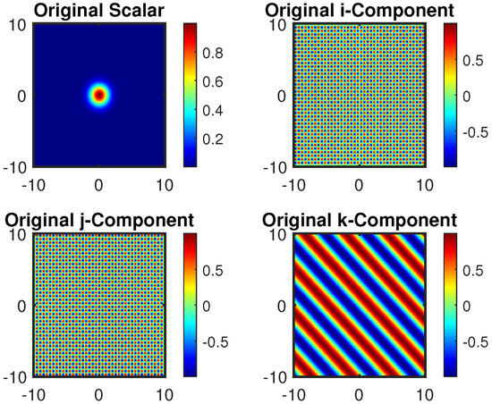
Figure 1.
Original signal.
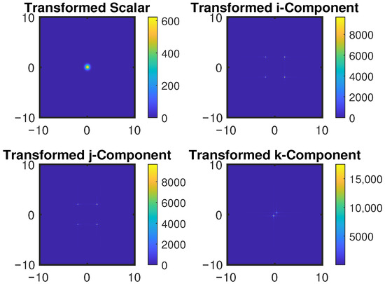
Figure 2.
Transformed signal.
4.2. Preservation of Inner Product
Proposition 1
(Inner Product Preservation). For any , the 2D QFRFT preserves the inner product, i.e.,
Proof.
From the explicit form of the kernel it follows that
Hence, the adjoint operator of satisfies
Since the inverse of the 2D QFRFT is given by , the transform is unitary on . Therefore, for all ,
This completes the proof. □
5. Modeling Probability Distributions with 2D QFRFT
5.1. From Continuous Theory to Finite-Grid Implementation
The 2D QFRFT is defined in Section 3 and Section 4 for functions , where both the spatial variables and the transform variables range over the entire plane . In practical numerical applications, however, signals are available only on finite discrete grids. We therefore briefly clarify how the continuous formulation fits into the finite-grid framework used in Section 5. In the numerical setting, a sampled signal
is interpreted as the restriction of a continuous function to a uniform sampling grid. Outside the sampling region, the signal is assumed to be extended by zero, which is equivalent to assuming compact support or sufficiently fast decay of f on . Under this assumption, the continuous QFRFT integrals are well approximated by finite Riemann sums. Accordingly, the continuous integrals in the definition of the 2D QFRFT are replaced by discrete summations over the sampled grid, and the transform variables are evaluated on a corresponding finite frequency grid. This discretized formulation constitutes a consistent numerical approximation of the continuous QFRFT and converges to the continuous transform as the grid resolution increases and the sampling window expands.
5.2. The Expected Value
The Expected Value of a discrete signal is a measure of its central tendency, weighted by the signal’s intensity. For a discrete signal , defined on a finite grid of points , the expected value is computed as:
where is the normalized probability distribution associated with the signal given by:
This normalization ensures that:
The expected value in the transform domain is given by:
where represents the squared magnitude of the transformed signal, and the probability distribution is:
Example 1.
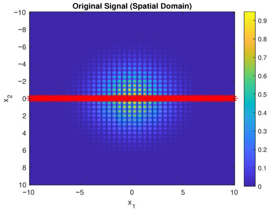
Consider a discrete 2D signal defined on a grid:
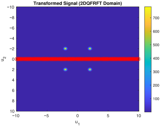
where . The signal is transformed using the 2D QFRFT with fractional orders and . The graphs generated in Figure 3 and Figure 4 show:
Figure 3.
Original signal in the spatial domain.
Figure 4.
Transformed signal in the 2D QFRFT domain.
- The original signal in the spatial domain.
- The transformed signal in the 2D QFRFT domain.
- The red line indicates the expected value in each domain.
Example 2.
Consider a signal where each sample represents a quaternion-like value. For simplicity, the quaternion components are represented as real numbers for the demonstration:
The signal is transformed using the 2D QFRFT with fractional orders and . The transformation is performed in accordance with (2). The magnitudes of the transformed signal components are calculated as:
where Re and Im denote the real and imaginary parts of the transformed components. The total magnitude is obtained by summing the magnitudes of all components:
The normalized probability corresponding to each component is expressed as:
This example demonstrates the application of the 2D QFRFT to a quaternion-valued signal, highlighting fractional frequency components, normalized probabilities, and energy distribution in the transform domain. As shown in Figure 5, the normalized probabilities represent the relative magnitudes of these components. Peaks indicate dominant spectral elements and reveal the signal’s energy distribution, while smaller values correspond to less significant contributions.
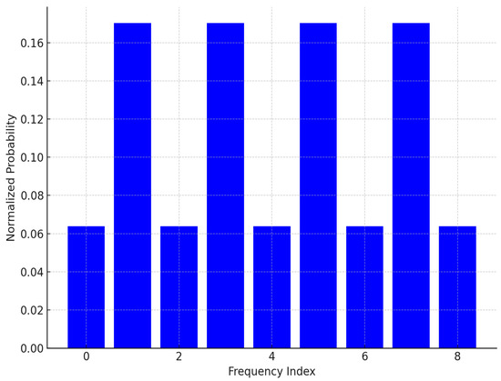
Figure 5.
Normalized probabilities in the 2D QFRFT domain.
6. 2D QFRFT in Signal Denoising
Signal denoising is crucial for accurately detecting and localizing useful information in the presence of noise and interference. Traditional methods often rely on Fourier-based techniques, which may struggle with multi-dimensional signals or noise patterns overlapping in the frequency domain. The 2D QFRFT provides a powerful alternative, leveraging its ability to analyze signals in the fractional domain.
To illustrate the practical utility of the proposed framework, we consider a radar signal as a representative example. This choice highlights how the 2D QFRFT can effectively denoise signals while preserving essential target features, though the approach is equally applicable to other domains of signal processing.
We demonstrate this with a simulated radar signal that represents targets at specific positions, superimposed with Gaussian noise. The following example outlines the detailed setup and parameterization of this signal.
Example 3.
Consider the following 2D radar signal representing targets at specific positions and noise distributed across the domain:
where
- : Amplitude of the k-th target.
- : Location of the k-th target.
- : Spread of the k-th target.
- : Gaussian noise.
We take specific parameter values: the number of targets , with amplitudes , , ; locations , , ; and spreads , , . The Gaussian noise has mean , variance , and standard deviation .
Substituting these values in the radar signal (14), we get
To compute the 2D QFRFT approximation for the radar signal (15), we have used the formula:
Remark 2.
The symbol “≈” in (16) denotes a numerical approximation of the continuous 2D QFRFT integral (2) obtained via discretization. This usage is restricted to numerical implementation and does not affect the theoretical definition of the 2D QFRFT. Specifically, when the signal is sampled on a finite grid with spacings and , the double integral in (2) is approximated by the corresponding double sum. The approximation becomes exact in the limit .
Figure 6 shows the original radar signal, while Figure 7 and Figure 8 highlight the transform’s magnitude and phase respectively, revealing energy concentrations and phase shifts.
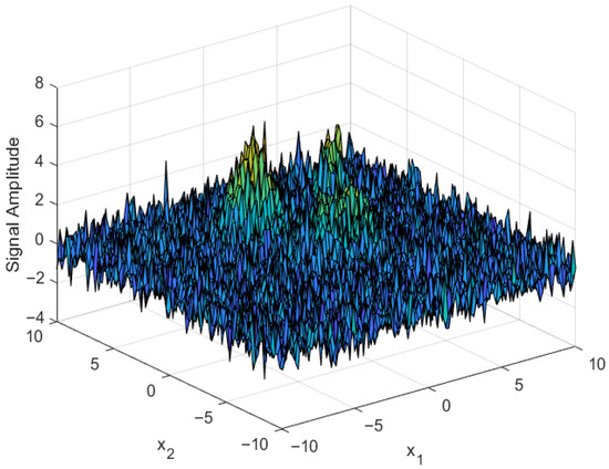
Figure 6.
Radar signal.
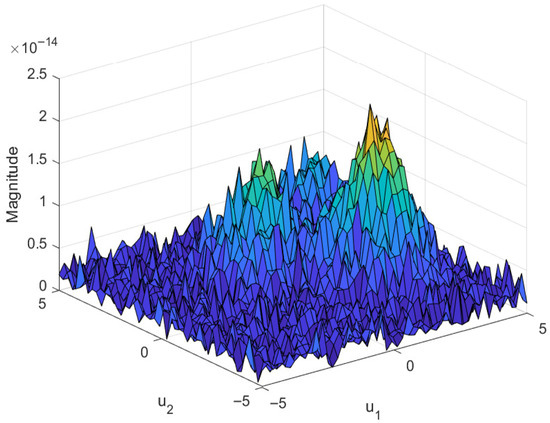
Figure 7.
Magnitude of the transformed signal.
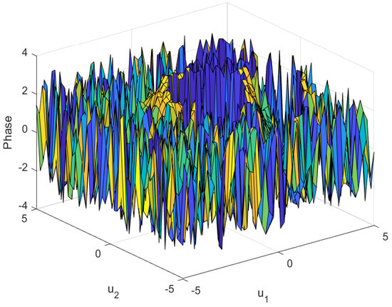
Figure 8.
Phase of the transformed signal.
The SNR (signal-to-noise ratio) is defined as:
where , the signal power, is the sum of squared amplitudes of the signal components:
and represents the noise. Moreover, the noise power is the sum of squared amplitudes of the noise:
Finally, let us introduce
where and represent the signal and noise powers, respectively, after applying the 2D QFRFT.
Figure 9 is dealing with the signal from Example 3. It is comparing the original SNR of the noisy radar signal with the transformed SNR, highlighting how the 2D QFRFT concentrates the signal’s energy and disperses noise in the transform domain.
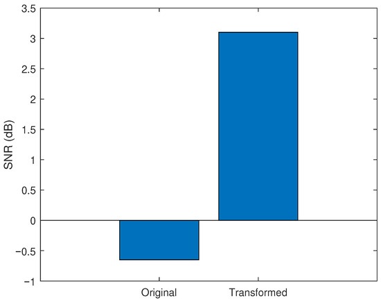
Figure 9.
SNR comparison.
7. Discussion and Analysis
The proposed 2D QFRFT provides a structured and mathematically consistent framework for analyzing quaternion-valued signals in the fractional domain. Unlike classical Fourier-based approaches, the 2D QFRFT enables independent fractional processing along each spatial dimension while preserving the non-commutative algebraic structure of quaternions. This feature is particularly significant for applications involving coupled multicomponent signals, where phase, orientation, and amplitude information must be handled simultaneously.
A key novelty of this work lies in the integration of probabilistic concepts directly within the 2D QFRFT domain. By deriving explicit expressions for normalized probability measures and expected values of quaternion-valued random variables, the proposed framework establishes a rigorous bridge between fractional transform theory and quaternion probability analysis. To the best of the authors’ knowledge, such probabilistic formulations in the 2D QFRFT domain have not been previously reported.
From an application perspective, the 2D QFRFT offers clear advantages in signal analysis tasks such as radar and imaging, where fractional-domain representations provide enhanced adaptability and resolution compared to integer-order transforms. The ability to selectively tune fractional orders in each dimension allows improved feature extraction and robustness against noise, as reflected in the presented simulations.
While the present study is intentionally restricted to the 2D case for theoretical clarity and practical relevance, the adopted tensor-product formulation suggests a natural pathway toward higher-dimensional generalizations. In this sense, the 2D QFRFT developed here serves as a foundational building block for future investigations into higher-dimensional QFRFT and their applications in non-commutative signal processing. Such extensions, however, are beyond the scope of the current work and are left for future research.
8. Conclusions
This paper has developed a theoretical framework for the 2D QFRFT and examined its role in multidimensional signal analysis and probability theory. By formally defining the transform and analyzing its action on quaternion-valued functions, fundamental results related to expected values and normalized probabilities were established in the 2D QFRFT domain. These findings extend existing quaternion transform theory to a fractional and two-dimensional setting.
Numerical experiments, including a radar signal example, were provided solely to illustrate the applicability of the proposed framework and to demonstrate its effectiveness in multidimensional signal representation. While not central to the theoretical development, these examples indicate the potential of the 2D QFRFT for practical signal analysis. Future work may focus on more comprehensive applications and simulations, particularly in biomedical signal processing, communication systems, and other areas where quaternion-based fractional transforms are relevant.
Author Contributions
M.A.S.: Writing—original draft, Investigation, Conceptualization, Methodology, Software. Z.Z.: Writing—review & editing, Validation. Y.X.: Formal analysis, Writing—review & editing. S.S.: Writing—original draft, Investigation, Conceptualization. M.Z.: Investigation & review. M.Y.B.: Investigation & review. All authors have read and agreed to the published version of the manuscript.
Funding
Mohra Zayed extends her appreciation to the Deanship of Research and Graduate Studies at King Khalid University for funding this work through Large Research Project under grant number RGP2/419/45.
Data Availability Statement
Data sets were not generated or analyzed during the current study.
Conflicts of Interest
The authors declare no competing interests.
References
- Chou, J.C.K. Quaternion kinematic and dynamic differential equations. IEEE Trans. Robot. Autom. 2020, 8, 53–64. [Google Scholar] [CrossRef]
- Took, C.C.; Mandic, D.P. The Quaternion LMS Algorithm for Adaptive Filtering of Hypercomplex Processes. IEEE Trans. Signal Process. 2009, 57, 1316–1327. [Google Scholar] [CrossRef]
- Xu, D.; Mandic, D.P. The Theory of Quaternion Matrix Derivatives. IEEE Trans. Signal Process. 2015, 63, 1543–1556. [Google Scholar] [CrossRef]
- Xiang, M.; Xia, Y.; Mandic, D.P. Performance Analysis of Deficient Length Quaternion Least Mean Square Adaptive Filters. IEEE Trans. Signal Process. 2020, 68, 65–80. [Google Scholar] [CrossRef]
- Fang-Jia, Y.; Li, B.Z. Spectral graph fractional Fourier transform for directed graphs and its application. Signal Process. 2023, 210, 109099. [Google Scholar] [CrossRef]
- Siddiqui, S.; Li, B.Z.; Samad, M.A. New Sampling Expansion Related to Derivatives in Quaternion Fourier Transform Domain. Mathematics 2022, 10, 1217. [Google Scholar] [CrossRef]
- Shi, J.; Zheng, J.; Liu, X.; Xiang, W.; Zhang, Q. Novel Short-Time Fractional Fourier Transform: Theory, Implementation, and Applications. IEEE Trans. Signal Process. 2020, 68, 3280–3295. [Google Scholar] [CrossRef]
- Zayed, A.I. On the relationship between the Fourier and fractional Fourier transforms. IEEE Signal Process. Lett. 1996, 3, 310–311. [Google Scholar] [CrossRef] [PubMed]
- Zayed, A.I. A convolution and product theorem for the fractional Fourier transform. IEEE Signal Process. Lett. 1998, 5, 101–103. [Google Scholar] [CrossRef]
- Koç, E.; Alikaşifoğlu, T.; Aras, A.C.; Koç, A. Trainable Fractional Fourier Transform. IEEE Signal Process. Lett. 2024, 31, 751–755. [Google Scholar] [CrossRef]
- Guanlei, X.; Xiaotong, W.; Xiaogang, X. Fractional quaternion Fourier transform, convolution and correlation. Signal Process. 2008, 88, 2511–2517. [Google Scholar] [CrossRef]
- Samad, M.A.; Xia, Y.; Siddiqui, S.; Bhat, M.Y. Two-dimensional quaternion linear canonical transform: A novel framework for probability modeling. J. Appl. Math. Comput. 2025, 71, 7493–7519. [Google Scholar] [CrossRef]
- Samad, S.S.M.A.; Ismoiljonovich, F.D. One dimensional quaternion linear canonical transform in probability theory. SIViP 2024, 18, 9419–9430. [Google Scholar] [CrossRef]
- Samad, M.A.; Xia, Y.; Al-Rashidi, N.; Siddiqui, S.; Bhat, M.Y.; Alshanbari, H.M. Generalized Sampling Theory in the Quaternion Domain: A Fractional Fourier Approach. Fractal Fract. 2024, 8, 748. [Google Scholar] [CrossRef]
- Li, Z.; Shi, H.; Qiao, Y. Two-sided fractional quaternion Fourier transform and its application. J. Inequal. Appl. 2021, 2021, 121. [Google Scholar] [CrossRef]
- Wei, D.; Li, Y. Different forms of Plancherel theorem for fractional quaternion Fourier transform. Optik 2013, 124, 6999–7002. [Google Scholar] [CrossRef]
- Irarrazaval, P.; Lizama, C.; Parot, V.; Sing-Long, C.; Tejos, C. The fractional Fourier transform and quadratic field magnetic resonance imaging. Comput. Math. Appl. 2011, 62, 1576–1590. [Google Scholar] [CrossRef]
- Roopkumar, R. Quaternionic fractional Fourier transform for Boehmians. Ukr. Math. J. 2020, 72, 942–952. [Google Scholar] [CrossRef]
- Kamalakkannan, R.; Roopkumar, R.; Zayed, A. Quaternionic Coupled Fractional Fourier Transform on Boehmians. In Sampling, Approximation, and Signal Analysis; Applied and Numerical Harmonic Analysis; Birkhäuser: Cham, Switzerland, 2023; pp. 453–468. [Google Scholar] [CrossRef]
- Hamilton, W.R. Elements of Quaternions; Longmans Green: London, UK, 1866. [Google Scholar]


Disclaimer/Publisher’s Note: The statements, opinions and data contained in all publications are solely those of the individual author(s) and contributor(s) and not of MDPI and/or the editor(s). MDPI and/or the editor(s) disclaim responsibility for any injury to people or property resulting from any ideas, methods, instructions or products referred to in the content. |
© 2026 by the authors. Licensee MDPI, Basel, Switzerland. This article is an open access article distributed under the terms and conditions of the Creative Commons Attribution (CC BY) license.