1. Introduction
The advantages of nonlinear energy sinks have been widely recognized [
1,
2,
3,
4]: they can achieve energy transfer through target energy transfer (abbreviated as TET) and dissipate most of the energy through NES damping. Under the context of TET, undesirable energy can be spatially transferred from a main structure to an attached NES in an irreversible way and efficiently dissipated. This irreversible energy transfer constitutes the core principle of vibration suppression in NES structures [
5]. The preceding research has paved the road for the final goal of optimization design for engineering applications. References [
6,
7] proposed an optimization method for the cubic stiffness of a cubic NES single-degree-of-freedom vibration system. The TET can be triggered when the initial energy value is higher than the optimization value. However, the author found during verification that the optimal stiffness designed in the literature cannot fully guarantee the effectiveness of all positions. Therefore, based on its optimization, this paper supplemented it to obtain a more reliable optimization method. To trigger TET, the initial energy needs to be greater than a fixed value, and NES needs to have a certain mass. Therefore, coupling into the main structure requires the introduction of a large additional mass, and the damping of the main structure is still the main factor in dissipating energy, which limits its practical application.
To overcome the problem of large additional mass, scholars have proposed the application of new structures, such as multiple NES parallel connections [
7,
8,
9,
10,
11] and lever-type NES [
12], which can effectively increase the vibration-reduction effect and possibly appropriately reduce the mass of NES, but obviously their structure is complex and increases the cost. With the emergence of inerters, research on the vibration suppression of integer-order inertial NES has begun to enter the field of view [
13,
14,
15]. In most of the related literature, the study still focuses on the effect of mechanical-type inerters [
16,
17] under ideal conditions, ignoring damping and nonlinear factors, which is equivalent to only considering the effect of inertia. A significant advancement was achieved by Swift et al. [
18], who pioneered a novel fluid inerter design utilizing a spiral tube as its core component. This architecture offers distinct advantages over mechanical counterparts, including structural simplicity, compact dimensions, high inertance, the elimination of backlash and eccentricity issues, and enhanced compatibility with diverse passive network layouts. While the dynamics of mechanical inerters are well-characterized (typically neglecting damping effects [
18,
19]), fluid inerters inherently exhibit damping behavior due to liquid viscosity and intrinsic structural properties. Consequently, research focus has shifted toward quantifying these damping mechanisms and even exploiting them for control purposes l [
20,
21,
22].
Existing models for fluid inerters predominantly rely on empirical formulations derived from classical experiments, often amalgamated through fitting procedures. Although simulations generally align with experimental data, discrepancies persist—particularly in low- versus high-frequency regimes [
23,
24]. This suggests limitations in fully capturing the underlying fluid dynamics. The apparent direct correspondence between components and flow behavior is an oversimplification; internally, fluid motion manifests complex phenomena. Whether laminar, turbulent, or transitional, localized flow structures exhibit fractal characteristics [
25], challenging conventional modeling paradigms. Therefore, after studying typical models of fluid inerters with different hypotheses [
23,
24], the author proposed two fractional-order inerter models and verified their effectiveness through comparison with classical experimental data and existing models. Using fractional-order models to describe fluid inerters also solves the theoretical research problem of traditional nonlinear models [
26]. This model only has one fractional derivative term that can simultaneously represent the inertia and damping characteristics of the fluid inerter. The model is more concise, and the parameter meanings are relatively clear. The fluid inerter expressed by the fractional-order model is called a fractional-order inerter. The author then applied fractional-order inerters to the study of critical damping in vibration isolation systems [
27] and the study of vibration characteristics in nonlinear energy sinks [
22].
This article will investigate the target energy transfer and energy dissipation mechanisms of NES with a fractional-order inerter, explore the influence of fractional-order inerter parameters, and compare the performance of different combinations of fractional-order inerter-based NES (abbreviated as FOIB-NES). The specific tasks of this article are as follows:
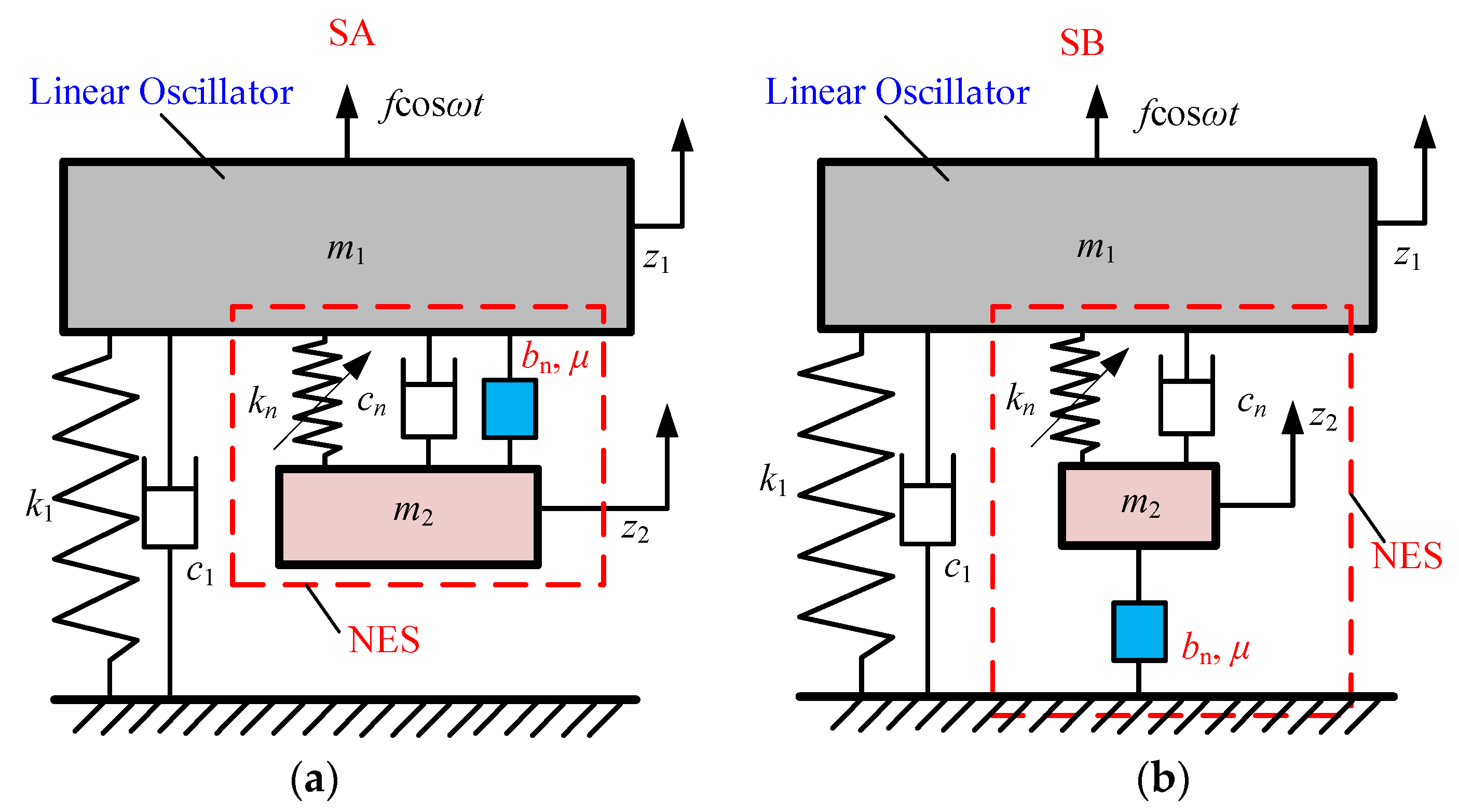
Section 2: Firstly, the single-degree-of-freedom vibration system models of coupled parallel and series FOIB-NES are presented. Using fractional-order properties to address the difficulties in applying the complex averaging method [
28,
29,
30,
31] to fractional-order nonlinear vibration systems, the slow-varying dynamic equations of the system are obtained, and the multi-scale method [
32,
33,
34,
35] is used to transform and further obtain the slow-varying manifold of the system.
Section 3: Firstly, based on the conclusions drawn in
Section 2, we derived the energy transfer relationship between the main oscillator and the NES oscillator. Then, we provided scenarios for triggering TET, optimal design criterion, and the influence of NES parameters on energy transfer, and summarized the optimal conditions for generating effective TET.
Section 4: In order to verify the reliability of the TET conditions proposed in
Section 3, (1) a comparison and verification of the energy transfer relationship with actual simulation results were provided for different initial energies and cubic stiffnesses; (2) and the corresponding energy dissipation curve of the main oscillator was provided to verify whether the dissipation capacity is stronger when TET is satisfied. (3) At the same time, different fractional-order dissipation curves were compared to verify that the fractional order has better dissipation ability. (4) To study the robustness or parameter margin of NES parameters, the dissipation time versus cubic stiffness curves were plotted for different inerter parameters and the robustness strength under different conditions was also discussed.
Section 5: The conclusion of the entire text is presented.
3. Analysis and Parameter Optimization of Target Energy Transfer
3.1. Deduction of Energy Transfer Relationship
To study the changes in the amplitude and phase trajectories of the oscillator in the equilibrium state of Scheme A, complex variables can be represented by modulus and phase angle [
7]:
Substitute Equation (27) into Equations (22) and (23) and make its real and imaginary parts zero to obtain the intermediate relationship equation. Then, simplify and organize it to obtain
For the convenience of analysis, further simplification is needed by introducing a dimensionless variable:
. From the definition of complex variables, we can note that
where
Ei0 is a conservative system with a dimensionless energy form like that of the main structure energy
E1, differing only by a multiple of 1/2. Therefore, Equation (28) can be transformed into
By following the same derivation steps as above, the energy relationship formula for Scheme B can be obtained
In the equation, variable H1 represents the energy of the primary oscillator, which approximates the energy of the linear main structure at multiple scales, and H2 represents a first-order approximation of the energy of the interaction between NES and the main structure at multiple scales. Obviously, H1 and H2 can be expressed as invariant manifolds of nonlinear modes at the time scale T0 → ∞, i.e., oscillator energy.
Observing the second Equations of (30) and (31), the energy dissipation rate relationship of the main structure of system A is relatively clear. When ξ1 = ξ2 = 0 and bn = 0 or ξ1 = ξ2 = 0 and μ = 2, ∂H1/∂T1 = 0, this is a conservative system, and the loss of non-existent energy must have a value of 0. When the factors related to dissipation are individually zero, the dissipation of energy is only related to non-zero damping. The right-hand end of the equation remains less than 0, indicating that the energy is constantly decreasing.
The energy dissipation rate relationship of the main structure of Scheme B system is relatively complex. When ξ1 = ξ2 = 0 and bn = 0 or ξ1 = ξ2 = 0 and μ = 2, ∂H1/∂T1 = 0 is consistent with Scheme A and is a conservative system. However, the influence of various damping needs further analysis.
3.2. The Generation Conditions of TET
Special note: During the simulation analysis below,
m1 = 10,
k1 = 0.6 remain unchanged, while the other parameters are suitable for discussion. Observing the first Equations of (30) and (31), both equations are very close to being cubic functions of
H1 with respect to
H2, and Scheme B has an additional coefficient of 1/(
2 +
2) compared to Scheme A. Since
= 1 +
λsin (
μ − 1) π/2, with
μ − 1 ∈ (0, 1),
> 1, it can be predicted that under the same parameter conditions, the
H1 amplitude of Scheme B will be smaller. A relationship diagram between
H1 and
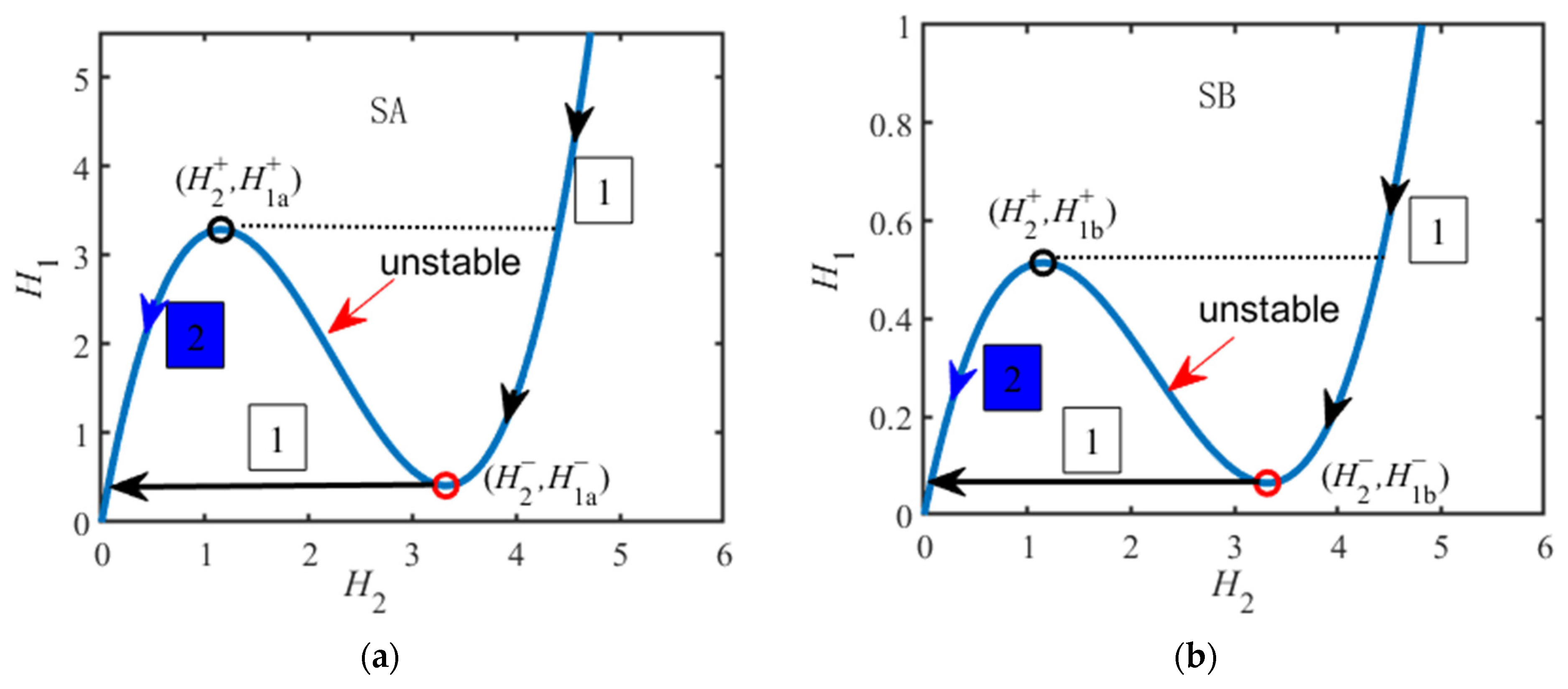
H2 was drawn based on these two equations, as shown in
Figure 2, with parameters
m2 = 0.3,
μ = 1.9,
c1 = 0.003,
cn = 0.002, and
bn = 0.4.
When there are three solutions for
H2 in
Figure 2, the line between two extreme points (black circles) and the peak valley (red circles) is unstable and easy to obtain. Due to the damping effect, the energy of the main structure is continuously dissipated, and the main energy is always in a decreasing state. Its flow must follow the direction of the black arrow route
1 or the blue arrow route
2 in the figure, rather than an unstable route, resulting in a unique jumping phenomenon in nonlinearity. This is also the cause of TET in the system. When the initial positions are different, the energy takes different routes [
6,
8].
By taking the derivative of
H2 in the first equation of Equations (30) and (31) and making it equal to zero, the expression for the extremum coordinates can be obtained as follows:
where
To study the relationship between damping and energy dissipation time in NES structures, it is necessary to determine all parameters except for the damping of the main structure. Therefore, the primary task is to design the structural parameters of NES. In addition to satisfying the condition of Equation (34), the parameters must be optimized. From
Figure 2 and Reference [
6], to achieve the optimal energy transfer method for NES, the following conditions must be met:
Among them,
E10 is the initial energy of the system’s main oscillator, calculated by Equation (29). So, a preliminary design can be carried out for its nonlinear stiffness
κ, with schemes a and b having
Although there are two routes in
Figure 2, the energy transfer of TET is a prerequisite for rapid energy dissipation. Obviously, route
1 is better, while route
2 is prone to monotonic decreases without jumping phenomenon. Therefore, only satisfying
H1(0) =
κH10(0) >
is problematic. When
H2(0) approaches route
2, the response is easily dropped into route
2. Therefore, to improve reliability, this article proposes, for the first time, a supplementary condition that the initial
H1(0) and
H2(0) should be above the maximum value and located to the right of the extreme value. Obviously, the two schemes have the same relationship equation
So far, the optimal design can be completed when the cubic stiffness meets these two equations, which can ensure the triggering of TET, but cannot guarantee the optimal energy dissipation performance. Therefore, other parameters of NES also need to be designed.
When the damping of the main structure
ξs = 0 and the NES damping ratio
ξ2 and the inerter parameters (
) jointly affect the energy transfer efficiency of the main structure (denoted as
Htransfer)
When resonance energy capture is at its optimal state, where all initial energy is transferred, there is
Deduction reveals that both schemes have the same
Hopt 3.3. Influences of NES Parameters on Energy Transfer
The expressions for
H1 and
H2 in schemes A and B are similar. Therefore, the influence of parameters on
H1 and
H2 is also consistent, except that
H1 in scheme B is
that of scheme A. Only Scheme A is shown below:
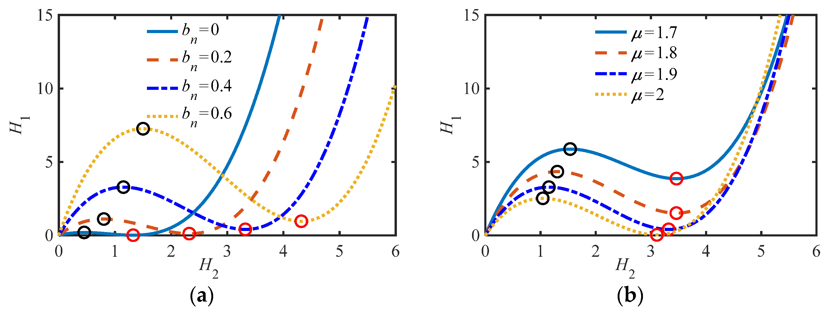
Figure 3 shows the relationship between
H1 and
H2 for different inertia coefficients bn (
μ = 1.9) and different fractional orders
μ (
bn = 0.4), where the circle in the figure is the extreme value of
H1 The remaining parameters are
m2 = 0.3,
kn = 0.12, and
cn = 0.002.
Overall,
bn has a significant impact on the amplitudes of
H1 and
H2, with
μ having a greater effect on
H1 and a relatively smaller effect on
H2. Under the same parameters, as
bn increases, the amplitudes of
H1 and
H2 become larger, and the height difference between the two extremes becomes greater. Combining
Figure 3a and Equation (35), the optimal cubic stiffness of the two schemes is significantly higher than that of the non-inerter NES (
bn = 0). Conversely, as
μ increases, the effect is the opposite. In addition, it was found that when using fractional-order inerters, the maximum value is greater than
bn = 0 (non-inerter NES), but the distance
between the two extreme values increases.
According to Equation (34), ∆p must be greater than or equal to 0. If all the parameters of the inerter are 0, we can obtain . Otherwise, we can simplify the inequality relationship: .
When
μ ∈ (5/3, 2), the size range of the cosine term on the right side of the inequality is cosπ/2~cos2π/3, which is obviously less than 0. Therefore, the critical damping (
) of FIOB-NES is larger than that of traditional NES, while the opposite is true when
μ∈ (1, 5/3). Based on the expression of ∆
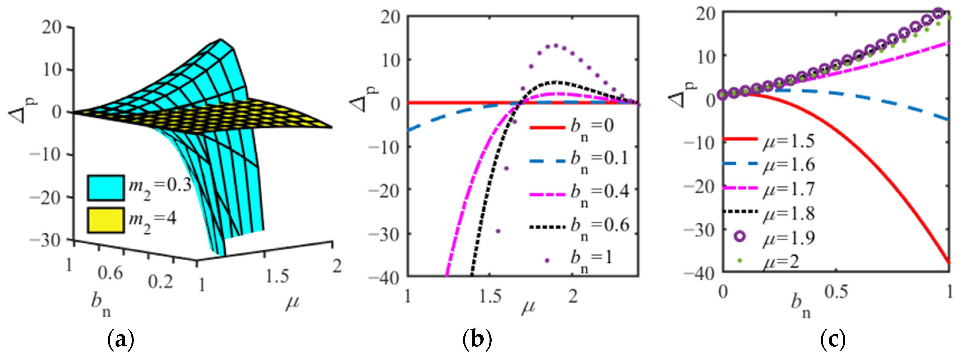
p, the relationship curve between parameters and ∆
p can be drawn as shown in
Figure 4 (other parameters: (a)
cn = 0.002; (b) and (c)
cn = 0.002 and
m2 = 0.3).
From
Figure 4a, as
m2 increases, ∆
p also increases.
Figure 4b shows that as
μ increases, ∆
p has a maximum value between 1 and 2 at
μ, and the location where ∆
p is greater than 0 is around
μ = 2. Furthermore, as
bn increases, ∆
p becomes relatively larger.
Figure 4c shows that
μ determines the influence of
bn; for example, when
μ = 1.5,
μ = 1.6,
bn cannot make ∆
p greater than 0 regardless of the value taken. When
μ = 1.7, 1.8, 1.9, and 2, the larger
bn, the larger ∆
p, indicating that the value of
μ determines the trend of ∆
p variation. The addition of fractional-order inerters can significantly alter the critical conditions of the original NES system.
It is obvious that ∆
p = 0 and
Htransfer = 0, and there is no energy transfer. Currently, the corresponding damping is called the critical value of energy transfer. Traditional NES (when
bn = 0,
= 0, and
= 0, then the critical value is
ξNES =
ξ2 <
is a constant). When introducing a fractional-order inerter, the energy transfer efficiency is not only related to NES damping
ξ2, but also to bn and
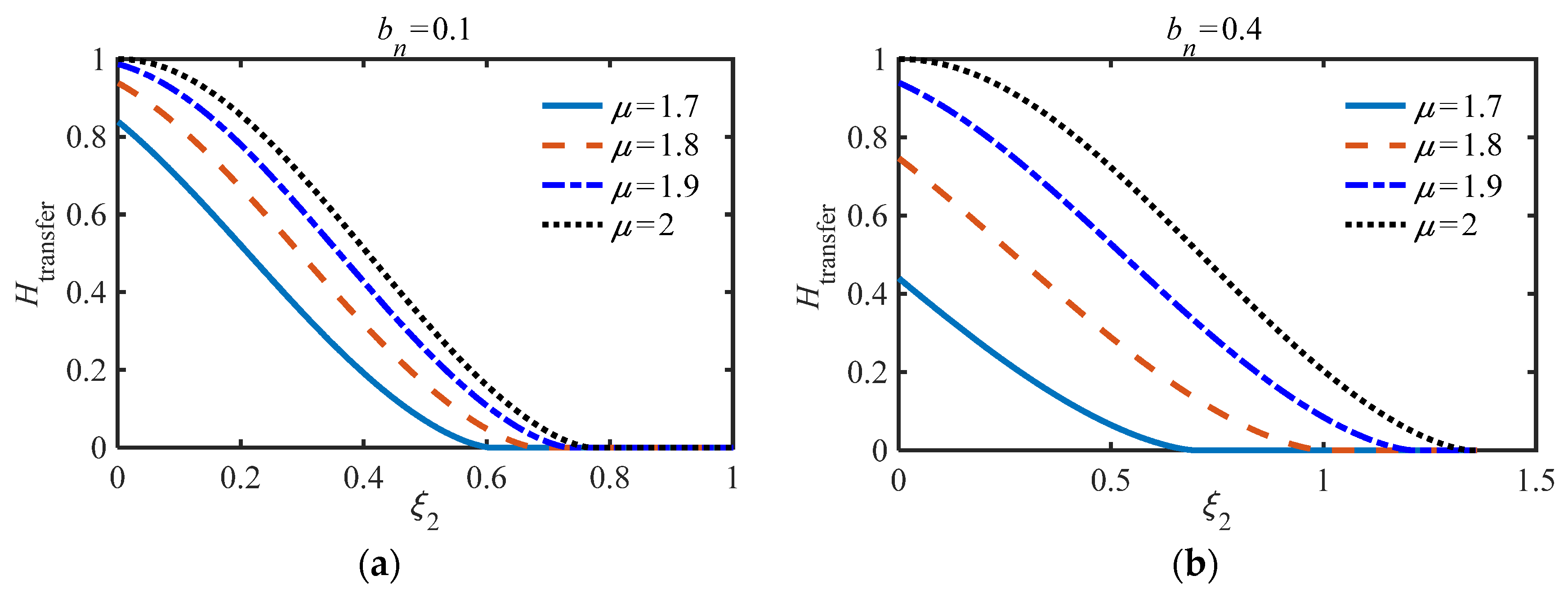
μ. The relationship curve between transfer efficiency and NES damping
ξ2 at different derivative orders
μ can be obtained from Equation (40) and
, as shown in
Figure 5a
bn = 0.1 and
Figure 5b
bn = 0.4. The critical damping value is located when the transfer efficiency is equal to 0 in the figure, and the value on the right side is meaningless and not plotted.
Figure 5 shows that the larger the
μ, the higher the efficiency for the same
ξ2, indicating that the damping attached to the fractional-order inerter is detrimental to energy transfer efficiency. When the order
μ is the same, the larger
bn, the greater the damping at which the transfer efficiency equals 0—that is, the greater the critical damping. However, with the same
ξ2, efficiency is significantly reduced. In summary, firstly, the damping
ξ2 of NES should be far away from the critical value, and the fractional order should be as close to 2 as possible. Finally, under the premise of meeting the requirements, choose a smaller
bn. When
ξ2 approaches or exceeds the critical damping, the energy transfer efficiency is almost zero, and other parameters cannot achieve TET. Here, we focus on the case of
cn = 0.002 (i.e.,
ξ2 = 0.027).
Based on the above analysis and discussion, the optimization conditions for generating effective TET are as follows: (1) ∆p >0; (2) NES damping cannot exceed the critical damping (the NES damping corresponding to a transfer efficiency of 0); (3) there exists an optimal minimum value κopt (i.e., threshold for triggering TET) for cubic stiffness (satisfying both Equations (36) and (37)); (4) while satisfying condition 2, try to choose the parameters that maximize the optimal energy transfer.
4. Discussion
Below, we will provide multiple typical simulation examples to verify the validity of the above conclusions. When the initial energy is concentrated in the main structure (i.e., z1 ≠ 0 or 1 ≠ 0, z2 = 0, 2 = 0), due to y1 = z1/, y2 = (z2 − z1)/, it can be seen from Equation (29) that H1(0) and H2(0) are not equal to 0.
All the original differential equations of the system are solved using the Runge–Kutta method, where the fractional-order terms are approximated by the Oustaloup approximation algorithm [
39]. The simulation time step is 0.1 and the duration is 1000 s. After obtaining the responses, they are converted into
H1(
τ1),
H2(
τ1), and
E1(
τ1) in the flow figures. When the analytical relationship between
H1 and
H2 (red thick solid line) and the comparison of numerical simulations with different initial energies
H1(0) and
H2(0) (initial conditions
ẏ1(0) = 0.4,
ẏ2(0) = −0.4) are given below, the conditions for the occurrence of jumps are verified. The cubic stiffness
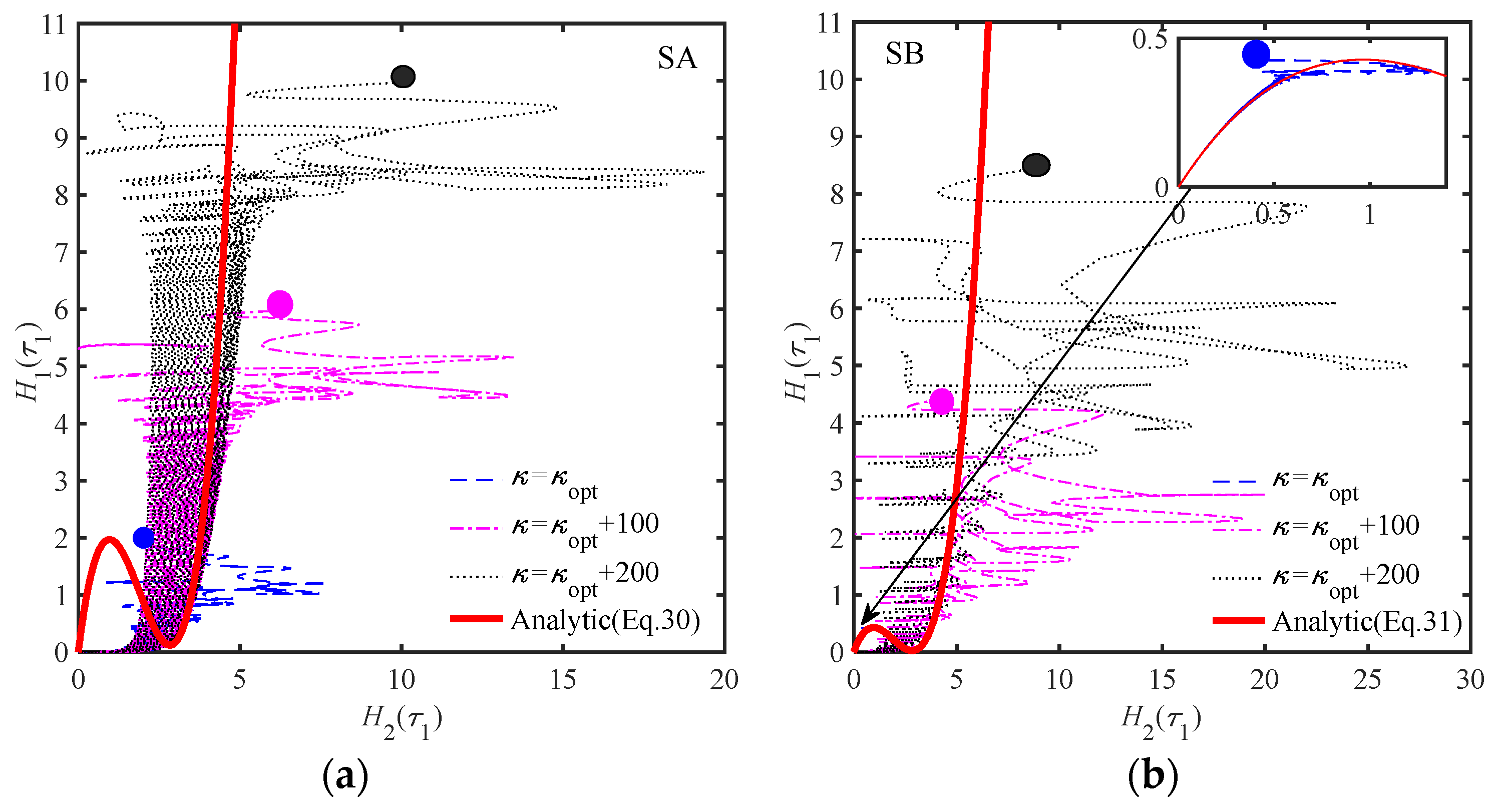
κ (calculated solely based on Equation (36)) corresponding to the four initial energies is shown in
Figure 6 and
Figure 7. At this point, the relationship between
H1(0) and
H2(0) is combined to satisfy the following inequality relationship.
For Scheme A:
- (1)
(solid line).
- (2)
(dashed line).
- (3)
(dotted line).
- (4)
(dash dot line)
For Scheme B:
- (1)
(solid line).
- (2)
(dashed line).
- (3)
(dotted line).
- (4)
(dash dot line).
The remaining parameters in
Figure 6 and
Figure 7 are
μ = 1.9,
m2 = 0.3,
bn = 0.3,
cs = 0, and
cn = 0.002. The circle in
Figure 6 clearly indicates the starting point of the energy response curve, and the following circles in
Figure 8 and Figure 10 are the same.
From
Figure 6, when Equation (36) is satisfied and the conditions of Equation (37) are also satisfied, both can go towards route
1. However, the dotted line in
Figure 6b, which satisfies the calculation of
κopt via Equation (36) but does not meet the conditions of Equation (37), requires route
2 is followed at this stage. If Equation (36) is not satisfied, we can only follow route
2 (as shown by the dashed line in
Figure 6).
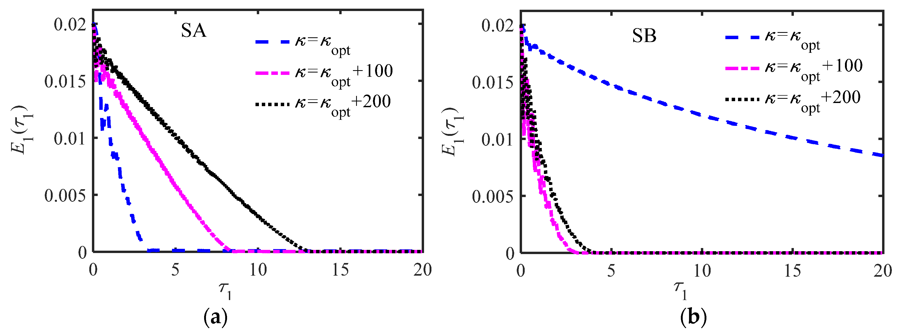
Figure 7 shows the time-domain response of the main structure energy (
E1 = 1/2
E10) for different
H1(0) and
H2(0): (a) Scheme A:
κopt = 12.3 and (b) Scheme B:
κopt = 2.68; all other parameters are the same as
Figure 7.
Figure 7 shows that there is a jump in the energy of the main oscillator along route 1, and the energy dissipation is fast; when following route 2, the energy dissipation of the main oscillator is very slow.
The second comparison is given below, with the same parameters of
m2 = 0.3,
bn = 0.3,
cs = 0, and
cn = 0.002. The initial conditions are changed to
ẏ1 (0) = 0.2,
ẏ2 (0) = −0.2,
H1 (0), and
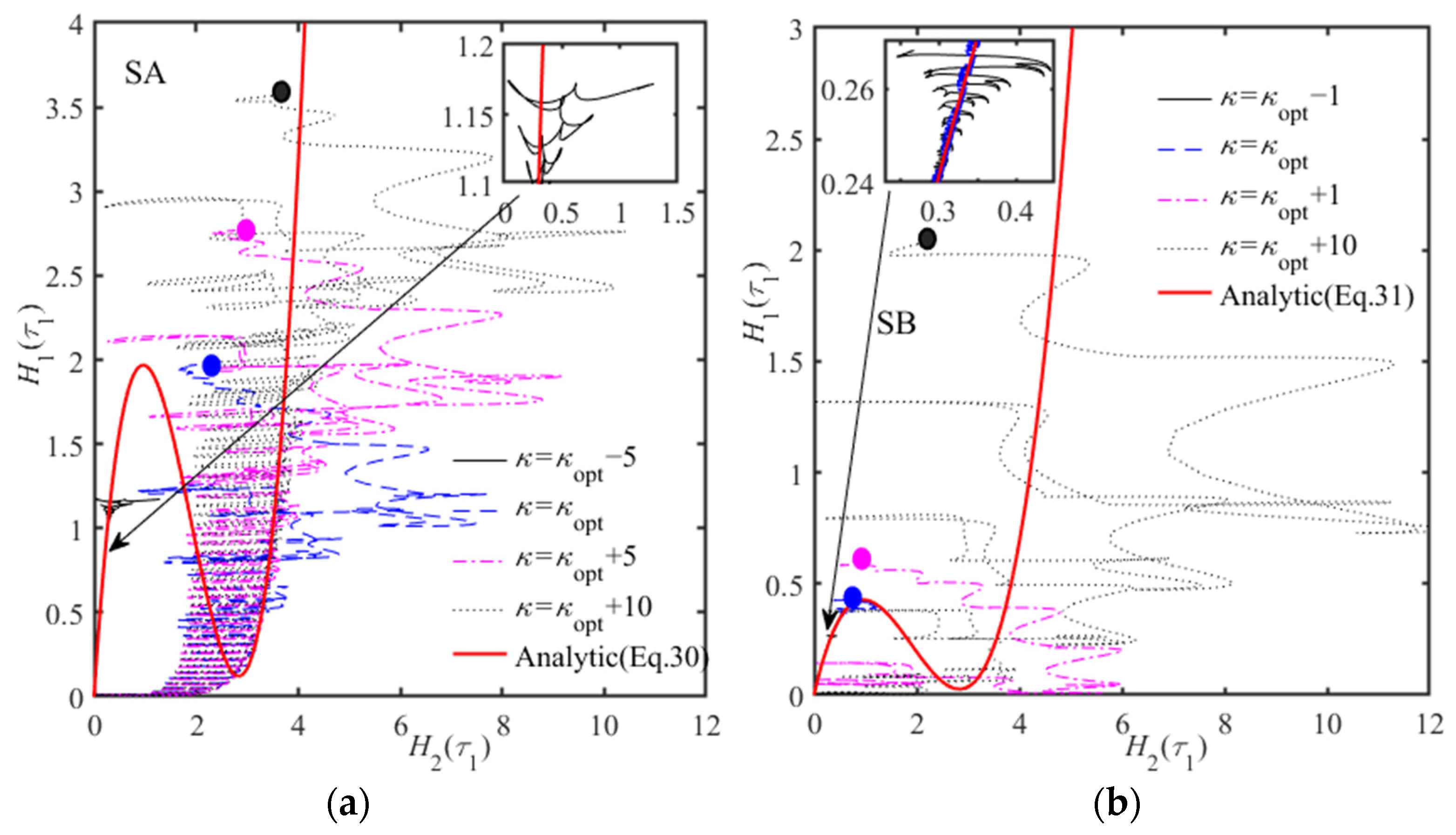
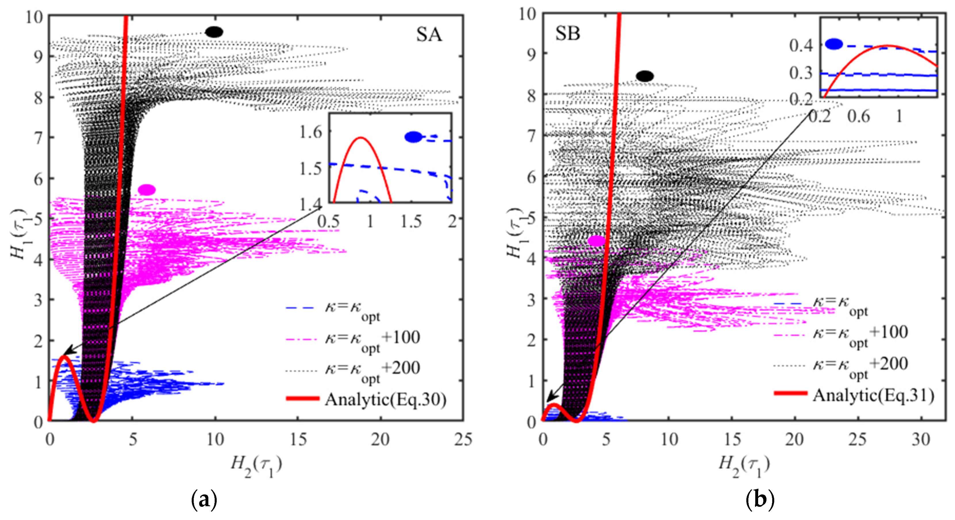
H2 (0) initial positions (dots) and cubic stiffness (as shown in the figures), and the remaining parameters in
Figure 8 and
Figure 9 are
μ = 1.9;
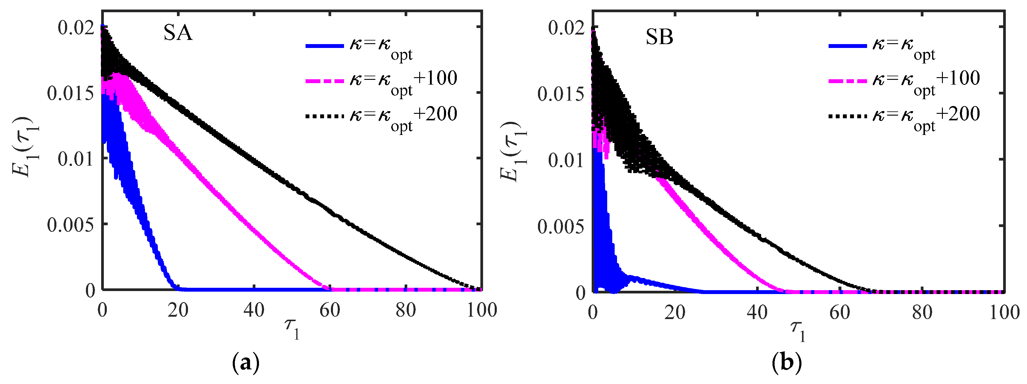
Figure 10 and
Figure 11 show
μ = 2.
Figure 8 and
Figure 9 show the case where a fractional-order inerter is used, where the blue dashed line in
Figure 8b only satisfies condition (36), resulting in traveling along route 2, while the others satisfy both inequalities simultaneously. Therefore, the energy of the main oscillator can only travel along route 1. The case where the cubic stiffness is much greater than the optimal value is also given. It can be seen from the figure that energy transfer and jumping can also occur when the initial energy is particularly large, and Scheme A has obvious energy transfer, but slower energy dissipation compared to Scheme B.
Figure 10 and
Figure 11 show the use of integer-order inerters, which significantly improve the transfer efficiency. The energy between the two oscillators is fully transferred, and jumps can also occur. However, the energy dissipation time of the main structure is obviously much longer than that of fractional-order inerters.
From the previous analysis, Scheme A, like traditional NES, basically needs to satisfy Equation (36) to achieve effective energy transfer and jump in most cases, while Scheme B needs to satisfy two conditional Equations (36) and (37) simultaneously to achieve it.
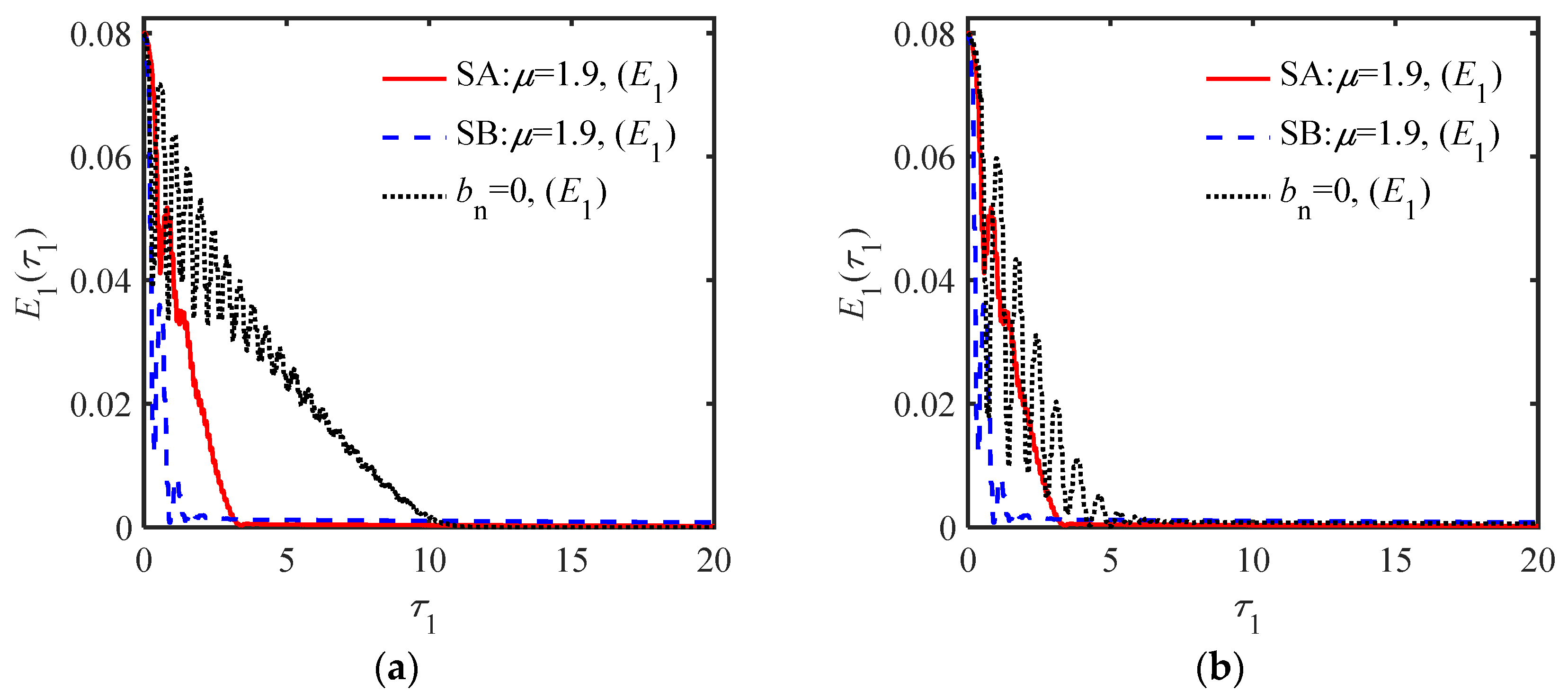
Figure 12 shows the comparison of the third group under the initial conditions of
ẏ1(0) = 0.4,
ẏ2(0) = −0.4. Two FOIB-NES schemes (
bn = 0.3) are compared with traditional NES (
bn = 0). When both SA and SB satisfy Equations (36) and (37) simultaneously, their
k values are taken as the optimal
κopt (with
κopt values of 12.3 and 6, respectively). The simulation results are shown in
Figure 12a,b. The traditional NES only satisfies Equation (36) (with
κopt =1.2), as shown in
Figure 12b, and
κ =
κopt +1.6 in
Figure 12a. The other parameters are
m2 = 0.3,
cs = 0, and
cn = 0.002.
From
Figure 12, Scheme B has the lowest number of energy transfers, but the fastest energy consumption. Scheme A shows a certain improvement compared to the non-inerter NES, but not significantly. Moreover, under the same initial energy, its cubic stiffness is the highest, and the non-inerter NES scheme has a particularly high transfer efficiency, but its dissipation capacity is clearly insufficient. Since the optimal stiffness of the non-inerter NES is only 1.2, it is prone to the influence of other nonlinear disturbances, as shown in
Figure 12a. When
κ = 2.8, its dissipation rate significantly decreases.
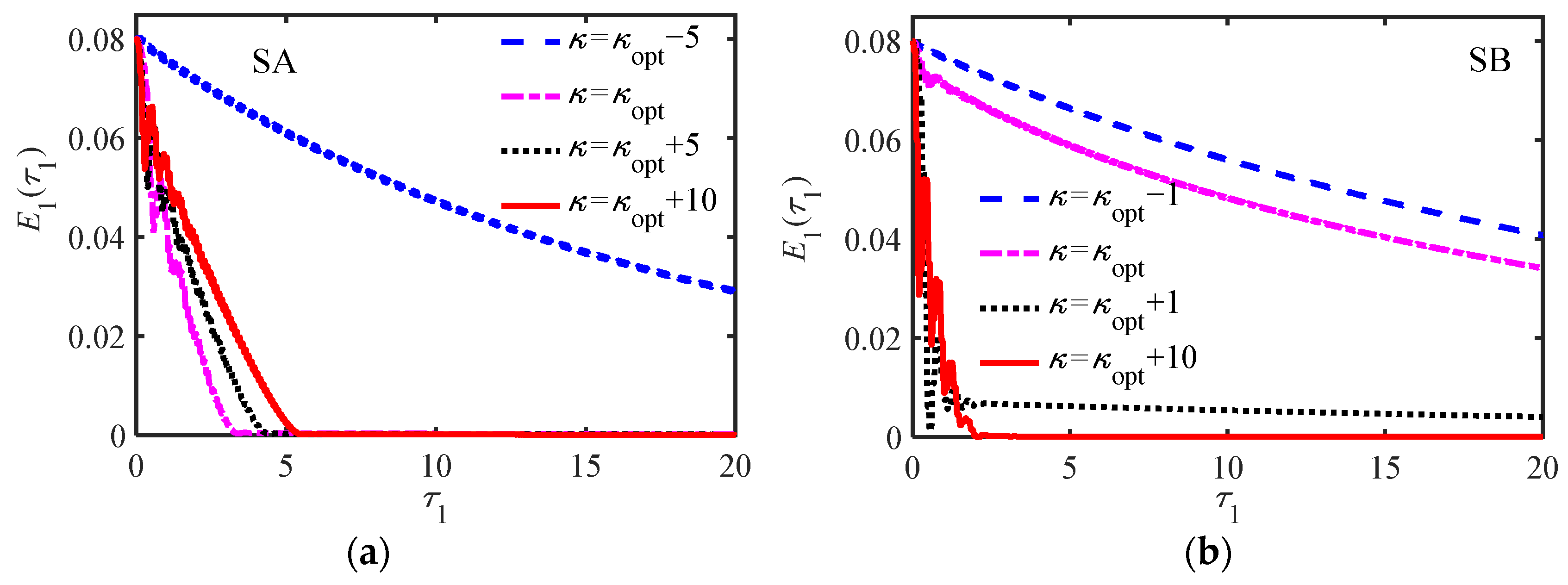
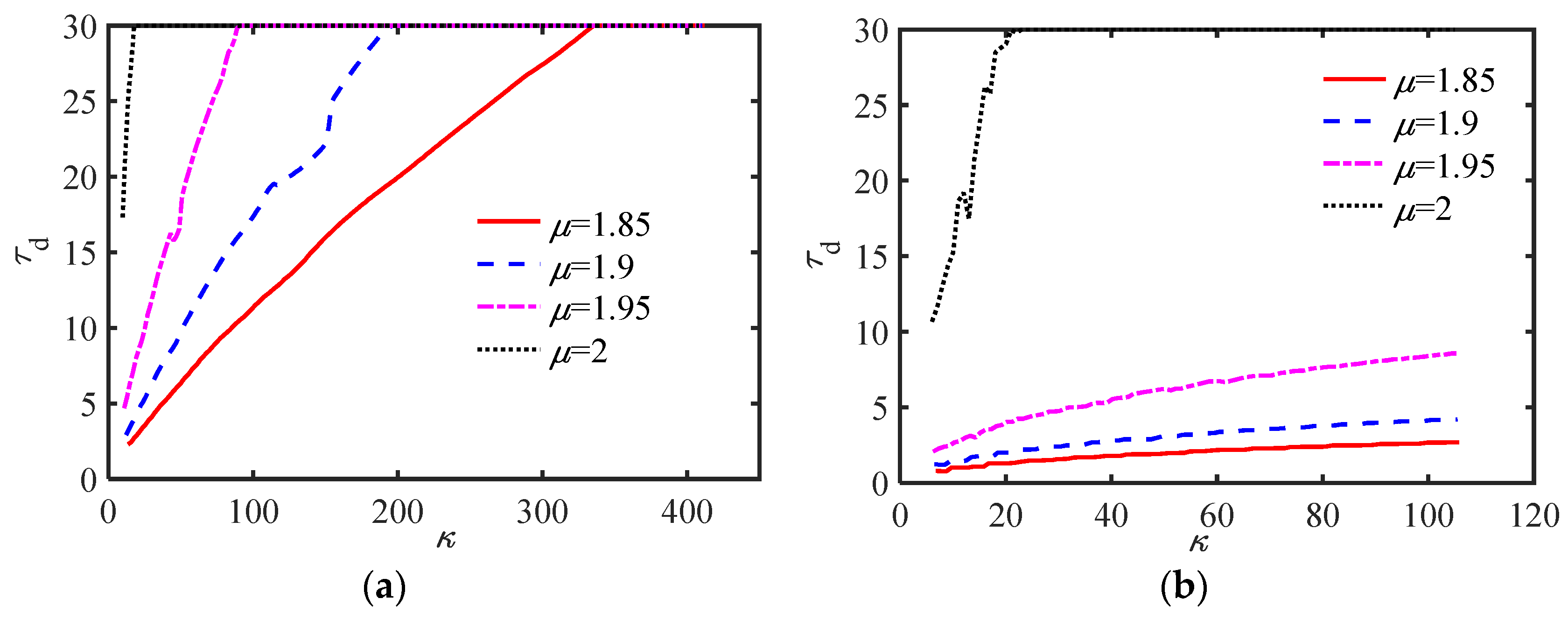
To study the robustness or parameter margin of the optimal cubic stiffness, a discriminant index is proposed based on the above analysis: dissipation time td, which corresponds to the time when the initial energy E1(0) dissipation of the main structure is 95% (η(τd) = 95%). The formula for the energy dissipation rate η(τ1) of the main structure is η(τ1) = [E1(0) − E1(τ1)]/E1(0) × 100%.
The optimal cubic stiffness value
kopt is selected as the starting point for simulation research, and then the cubic stiffness is increased by a step size of 1 (SB) and 0.5 (SB) to output the dissipation time curves of two different schemes with different orders and
η(
τd) = 95% as shown in
Figure 13 (the parameters, except for
k and
μ, are consistent with
Figure 12). Special note: The simulation time for the following example is 30 s. In the area where
τd reaches 30 s in the figure, the actual
τd is already greater than 30 s, and TET is basically ineffective. Therefore, to save computational costs,
τd is uniformly taken as 30 s.
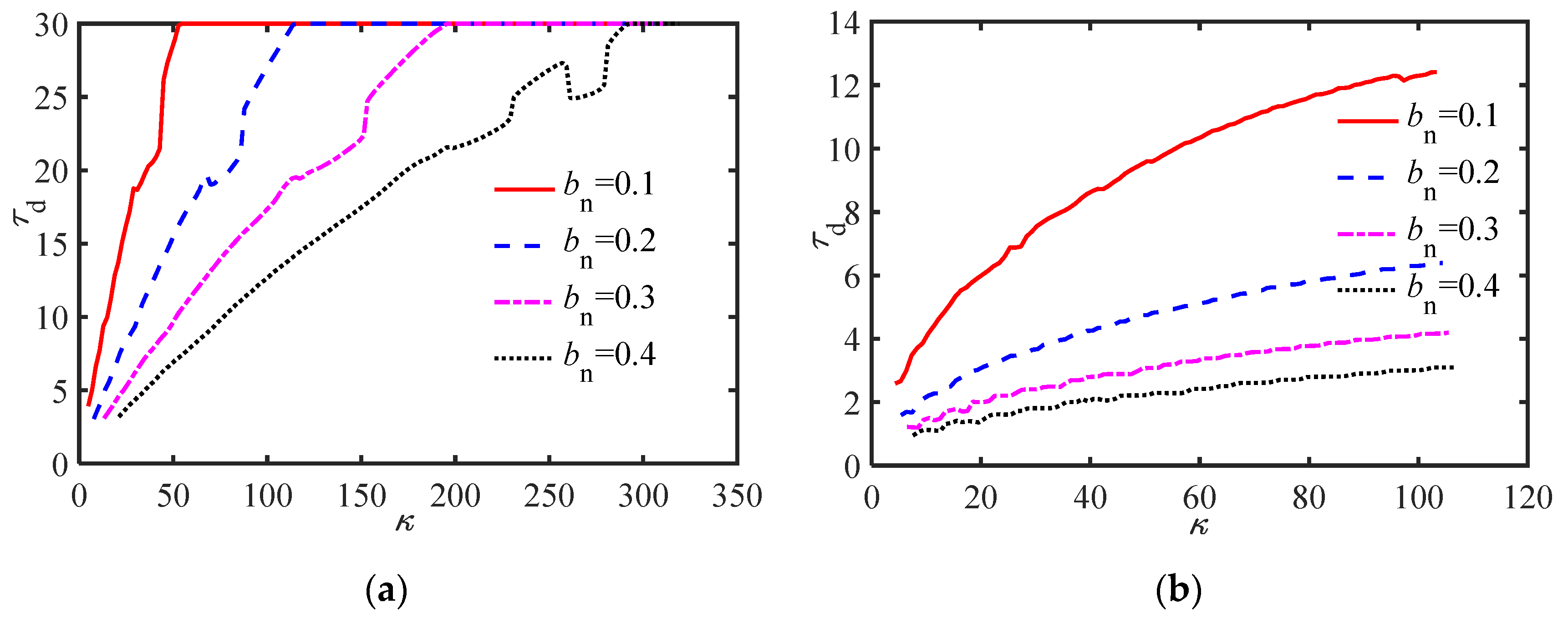
Similarly, we also plotted the dissipation time curves (
μ = 1.9) for different inertance
bn, as shown in
Figure 14.
Figure 13 and
Figure 14 show that the dissipation time and robustness of the inerter of fractional order are significantly better than those with
μ = 2, and scheme B is better than scheme A. In addition, the smaller the
μ, the better the robustness, while the larger the
bn, the better the robustness.
From the above simulation comparison and discussion, the following results can be drawn:
- (1)
When Equation (36) is mostly satisfied, it is effective, especially for scheme A and traditional NES without inerters, while Scheme B will follow route
2, as shown in
Figure 6b and
Figure 8b.
- (2)
Figure 7 and
Figure 9 show that the energy of the main structure decreases very slowly when traveling along route
2, without jumping, monotonically decreasing. However, when traveling along route
1, both schemes can quickly decrease and then jump to a lower position towards 0.
- (3)
After meeting the TET conditions, the higher the transmission efficiency, the lower the dissipation capacity, which is only a prerequisite for effectively suppressing vibration. Further research is needed on the speed of dissipation. When using an integer-order inerter, as shown in
Figure 10, both schemes follow route
1 and have sufficient transmission. However, from
Figure 11, the energy drop rate is much slower than in
Figure 9.
- (4)
At the same initial velocity, the optimal cubic stiffness
κopt, required for TET generation in Scheme A, is much larger than that in Scheme B, while the
κopt is minimized in integer-order inertial NES. In addition, from
Figure 13 and
Figure 14, scheme B has better parameter robustness than scheme A, and both schemes are more robust than integer-order when using fractional-order inerters.
In summary, the conditions for generating TET are as follows: satisfy the inequality of Equation (34), ensuring that the equation has multiple roots; simultaneously satisfy the inequalities of Equations (36) and (37), and try to take values near the lower limit to ensure the occurrence of jumps; keep NES damping away from the critical damping to ensure a certain transmission efficiency; considering the energy dissipation capacity, it is necessary to select smaller values of ξ2 and a larger values of bn, and to select a value of μ that is less than but close to 2.