Modeling Pandemic Dynamics via Fuzzy Fractional SEIQR Framework with ABC Derivatives: Qualitative Analysis and Computational Approaches

Abstract

Epidemic modeling plays a crucial role in understanding disease transmission and informing public health strategies. This study presents a fractional Susceptible-Exposed-Infected-Quarantined-Recovered (SEIQR) model incorporating Atangana–Baleanu-Caputo (ABC) fractional derivatives to capture memory effects in disease dynamics. The model extends classical ordinary differential equation-based frameworks by integrating a fractional approach, enhancing its applicability to real-world epidemic scenarios. A key feature of our model is the inclusion of mortality rates across all disease compartments, providing a refined representation of influenza-like infections with pandemic potential. We conduct a detailed stability analysis to assess equilibrium states and derive conditions for disease control. Numerical simulations further validate the theoretical findings, offering insights into epidemic progression and intervention strategies. Our results highlight the significance of fractional calculus in epidemiological modeling and its potential to improve predictive accuracy for infectious disease outbreaks.

1. Introduction

The persistence and spread of viral diseases remain a major global concern. The wide distribution of viral pathogens means that virtually everyone is susceptible to at least one seasonal illness. Transmission commonly occurs through contact with infected individuals, air, or water, underlining the challenge of controlling outbreaks.

Mathematical modeling utilizing different methods [1] plays a pivotal role in understanding and predicting the behavior of infectious diseases [2]. In particular, in fractional calculus—comprising derivatives, piecewise differential operators and integrals of non-integer order—has emerged as a robust tool for modeling complex dynamical systems, such as epidemics, due to its capacity to capture memory effects and hereditary properties, factors overlooked by classical integer-order approaches [3,4,5]. Among these, the Atangana–Baleanu (ABC) fractional derivative stands out for its non-singular and non-local kernel, offering enhanced accuracy and stability, particularly in biological and epidemiological models [2]. Incorporating fuzzy logic into fractional differential modeling enables handling of uncertainties and imprecision within real-world epidemic data and parameters [6]. Thus, integrating fuzzy logic with ABC fractional derivatives in the SEIQR model facilitates a comprehensive and robust framework capable of realistically capturing pandemic spread and informing control measures.

The history of influenza and related viral epidemics demonstrates the significant impact and evolving nature of such diseases. Notably, the 1918 flu pandemic marked a milestone, accompanied by recurring large-scale outbreaks over the past century. Diseases such as Swine Flu (H1N1) and COVID-19 exemplify the devastation caused by novel and re-emergent viral strains [7]. These events highlight the urgency of developing reliable mathematical models to analyze and forecast epidemic trends.

Differential equations constitute the backbone of epidemic modeling, and contemporary approaches extend to multiple frameworks, including symmetry-based models, time-invariant parameters, and network-based structures [8,9]. Research devoted to the mathematical and computational study of epidemics continues to expand, particularly regarding new viral strains and the integration of advanced mathematical tools [10]. For a comprehensive review of historical pandemics and their spread, see [7].

To address the lack of models accounting for memory effects and uncertainties, previous works have considered diverse methodologies. These include the development of fractional epidemic models, innovations in numerical methods [11], and the incorporation of fuzzy frameworks [1,3,12,13]. Recent studies have also employed stochastic modeling and machine learning techniques for analyzing and predicting epidemic dynamics [14,15].

Foundational insights into numerical analysis were provided in [16]. Stability modifications in the SIR model were investigated in [11,17]. The mathematical theory of epidemics was initially presented in [18], with further contributions from Allen [19]. Machine learning techniques for COVID-19 classification based on amino acid encoding were employed in [14]. The effectiveness of stability analysis and existence of solutions for a modified fractional SIRD COVID-19 model were studied in [20].

Under lockdown conditions, the dynamics of COVID-19 in India were examined in [21]. A discrete stochastic model for COVID-19 was provided in [22], and the impact of diagnostic delays on transmission was addressed in [23]. Stability investigation of fractional systems with the Riemann–Liouville derivative was supplied by Qian et al. in [24]. Asymptotic carriers in dengue transmission dynamics with control interventions were detailed in [25]. Forecasting of delayed SEIQ pandemic dynamics was explored in [26]. Periodic boundary value problems for fractional differential equations with the Riemann–Liouville derivative were investigated in [27]. Finally, both finite-time stability analysis and control of stochastic SIR epidemic models, particularly concerning COVID-19, were studied in [15].

Fuzzy set theory, first introduced in 1965, addresses vagueness and ambiguity where crisp boundaries between states do not exist [28]. By applying membership functions and fuzzy inference systems, fuzzy differential equations extend ordinary differential equations to incorporate imprecise or uncertain information, reflecting real-world complexities in epidemic data and modeling. The process of modeling with fuzzy logic involves formalizing membership functions, defining fuzzy rules, conducting fuzzification and defuzzification, discretizing relevant parameters, and choosing numerical solution methods tailored to the specific application.

This study develops a novel fractional SEIQR epidemic model that uniquely integrates fuzzy logic with the Atangana–Baleanu-Caputo (ABC) derivative, an approach seldom explored in the context of pandemic modeling. The model makes explicit provision for mortality in all compartments, thereby enhancing its relevance for influenza-like diseases. Analytical investigations focus on stability and disease control thresholds amid fuzzy and fractional uncertainties, while efficient numerical simulation approaches are used to validate the theoretical findings and provide forecasts for epidemic trends and intervention effectiveness. Compared with conventional integer-order or crisp models, this approach underscores the potential of fuzzy fractional calculus in epidemiology.

The organization of the paper is as follows: In Section 2, Section 3, Section 4, Section 5 and Section 6, the work presents model formulation, essential background, analytical study, simulation results, conclusion, and discussion, respectively.

2. Epidemic Model SEIQR-Formulation

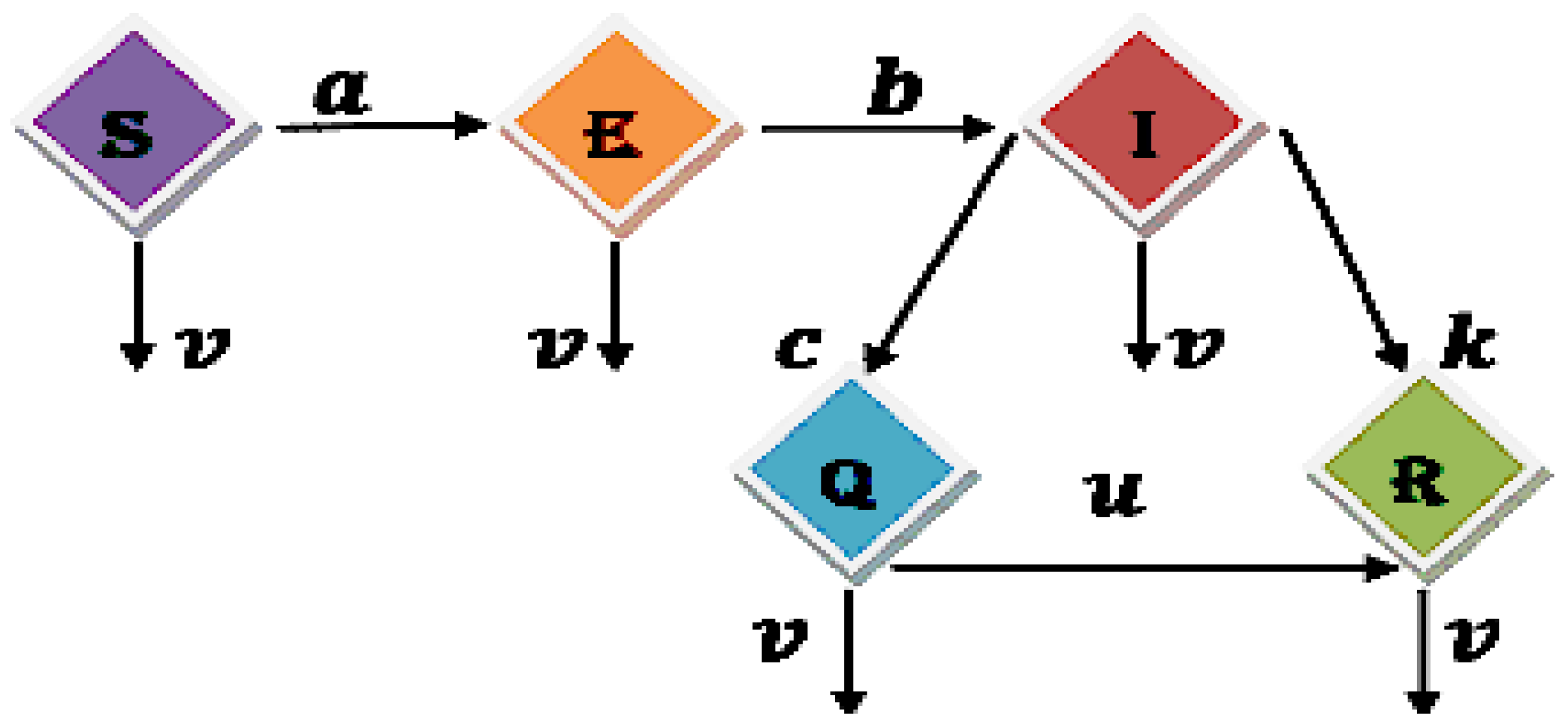
The objective of this study is to develop a novel epidemic model, termed the SEIQR model, which incorporates various prevalent and potentially fatal flu-like infections. As depicted in Figure 1, individuals migrate between compartments within the SEIQR framework. The rates of transition between these compartments are represented by the variables $a,b,c,\dots ,v$, corresponding to each compartment in sequential order.

Let $S\left(t\right)$, $E\left(t\right)$, $I\left(t\right)$, $Q\left(t\right)$, and $R\left(t\right)$ denote the densities (or proportions) of the Susceptible, Exposed, Infected (infectious), Quaranteed, and Recovered subpopulations at time $t\ge 0$, respectively, where the total population satisfies $N\left(t\right)=S\left(t\right)+E\left(t\right)+I\left(t\right)+Q\left(t\right)+R\left(t\right)$.

Any population compartment function $S,E,I,Q,R$ are considered in the place of $S\left(t\right),···,R\left(t\right)$, respectively, for convenience.

$$\begin{array}{ccc}{S}^{\prime }\left(t\right)& =& -aS\left(t\right)E\left(t\right)-vS\left(t\right)\hfill \\ E^{\prime }\left(t\right)& =& aS\left(t\right)E\left(t\right)-bE\left(t\right)I\left(t\right)-vE\left(t\right)\hfill \\ I^{\prime }\left(t\right)& =& bE\left(t\right)I\left(t\right)-cI\left(t\right)Q\left(t\right)-kI\left(t\right)-vI\left(t\right)\hfill \\ Q^{\prime }\left(t\right)& =& cI\left(t\right)Q\left(t\right)-uQ\left(t\right)R\left(t\right)-vQ\left(t\right)\hfill \\ R^{\prime }\left(t\right)& =& uQ\left(t\right)R\left(t\right)+kI\left(t\right)-vR\left(t\right)\hfill \end{array}$$

(1)

3. Preliminaries

For the benefit of readers, we highlight several important results on fractional differential equation (FDE) using the ABC derivative framework.

Definition 1

(Refs. [6,8,9] Atangana–Baleanu–Caputo (ABC) fractional derivative). Let $0<\alpha <1$ and $T>0$, and assume that $f:[0,T]\to \mathbb{R}$ is an absolutely continuous function. The ABC fractional derivative of order α is defined as follows:

$${}_{ABC}D_{0,t}^{\alpha }f\left(t\right)={\displaystyle \frac{F\left(\alpha \right)}{1-\alpha }}{\int }_0^t{f}^{\prime }\left(\mu \right)E_{\alpha }\left(-{\displaystyle \frac{\alpha }{1-\alpha }}{(t-\mu )}^{\alpha }\right)d\mu ,$$

(2)

where

• ${\displaystyle E_{\alpha }\left(z\right)=\sum _{k=0}^{\infty }\frac{z^k}{\Gamma (\alpha k+1)}}$ is the one-parameter Mittag–Leffler function;
• $F\left(\alpha \right)$ is a normalization function such that $F\left(0\right)=F\left(1\right)=1$.

Definition 2

(Refs. [6,8,9] Laplace transform of the ABC fractional derivative). Let $\mathcal{L}\left\{f\right(t\left)\right\}\left(s\right)=F\left(s\right)$ denote the Laplace transform of f. For $0<\alpha <1$, the Laplace transform of the ABC fractional derivative defined in (2) is given by

$$\mathcal{L}\left\{{}_{ABC}D_{0,t}^{\alpha }f\left(t\right)\right\}\left(s\right)={\displaystyle \frac{F\left(\alpha \right)}{1-\alpha }}{\displaystyle \frac{s^{\alpha }F\left(s\right)-s^{\alpha -1}f\left(0\right)}{s^{\alpha }+\frac{\alpha }{1-\alpha }}}.$$

(3)

Furthermore, in the limit $\alpha \to 1^{-}$, one obtains

$$\underset{\alpha \to 1^{-}}{lim}\mathcal{L}\left\{{}_{ABC}D_{0,t}^{\alpha }f\left(t\right)\right\}\left(s\right)=sF\left(s\right)-f\left(0\right),$$

which is the Laplace transform of the classical Caputo derivative.

Definition 3

(Refs. [6,8,9] Atangana–Baleanu fractional integral). Let $\alpha >0$ and let $f:[0,T]\to \mathbb{R}$ be any integrable function. The Atangana–Baleanu fractional integral of order α is defined by

$${}^{AB}J_{0,t}^{\alpha }f\left(t\right)={\displaystyle \frac{1-\alpha }{F\left(\alpha \right)}}f\left(t\right)+{\displaystyle \frac{\alpha }{F\left(\alpha \right)\Gamma \left(\alpha \right)}}{\int }_0^t{(t-\mu )}^{\alpha -1}f\left(\mu \right)d\mu ,$$

(4)

where $F\left(\alpha \right)$ is the same normalization function used in the ABC derivative, satisfying $F\left(0\right)=F\left(1\right)=1$. As $\alpha \to 1$, one has

$$\underset{\alpha \to 1}{lim}{}^{AB}J_{0,t}^{\alpha }f\left(t\right)={\int }_0^{t}f\left(\mu \right)d\mu ,$$

so the classical integral is recovered.

We convert system (1) to the following FDE, as shown in System (5):

$$\begin{array}{ccc}{}_{ABC}S^{{\alpha }_1}\left(t\right)& =& -aS\left(t\right)E\left(t\right)-vS\left(t\right),\hfill \\ {}_{ABC}E^{{\alpha }_2}\left(t\right)& =& aS\left(t\right)E\left(t\right)-bE\left(t\right)I\left(t\right)-vE\left(t\right),\hfill \\ {}_{ABC}I^{{\alpha }_3}\left(t\right)& =& bE\left(t\right)I\left(t\right)-cI\left(t\right)Q\left(t\right)-kI\left(t\right)-vI\left(t\right),\hfill \\ {}_{ABC}Q^{{\alpha }_4}\left(t\right)& =& cI\left(t\right)Q\left(t\right)-uQ\left(t\right)R\left(t\right)-vQ\left(t\right),\hfill \\ {}_{ABC}R^{{\alpha }_5}\left(t\right)& =& uQ\left(t\right)R\left(t\right)+kI\left(t\right)-vR\left(t\right).\hfill \end{array}$$

(5)

The fulfillment of initial conditions implies a constant net population size N, given by

$$S\left(0\right)+E\left(0\right)+I\left(0\right)+Q\left(0\right)+R\left(0\right)=N.$$

The population count of $S,E,I,Q,R$ are initially considered as $n_1,n_2,n_3,n_4,n_5$, and all of them equated to 100, i.e., $S\left(t\right)=n_1=100=\dots =R\left(t\right)=n_5=100$.

In System (5), the fractional orders are denoted as ${\alpha }_1,{\alpha }_2,{\alpha }_3,{\alpha }_4,{\alpha }_5\in [0,1]$, corresponding to the Susceptible (S), Exposed (E), Infected (I), Quarantined (Q), and Recovered (R) compartments, respectively. This flexible multi-order framework allows for independent variation in each compartment’s fractional derivative order, enabling comprehensive analysis of heterogeneous memory effects across subpopulations.

While traditional studies often fix a single uniform order $\alpha \in [0,1]$ across all compartments, our approach facilitates richer dynamical exploration. For instance, the Susceptible dynamics can be examined at ${\alpha }_1=0.2$ while simultaneously investigating Exposed behavior at ${\alpha }_2=0.1$ or $0.3$, and analogous flexibility applies to other compartments. Each ${\alpha }_i$ governs the memory effects specific to its respective subpopulation, revealing compartment-specific fractional dynamics unattainable with uniform ordering.

This multi-fractional structure provides mathematical flexibility to study diverse epidemic scenarios, capturing varying hereditary influences on different disease stages and offering deeper insights into SEIQR model behavior compared to single-order formulations.

The parameter values of Susceptible-Exposed $\left(a\right)$, Exposed-Infected $\left(b\right)$, Infected-Quarantined $\left(c\right)$, Infected-Recovered $\left(k\right)$, Quarantined-Recovered $\left(u\right)$, and Death $\left(v\right)$ used in all equations are, respectively, $0.009,0.007,0.005,0.001,0.004,$ and $0.4.$

In epidemic modeling, fuzzy approaches are compelling for representing uncertainties inherent in parameters and population states. For instance, compartmental functions, $\left(S\right(t),E(t),I(t),Q(t),R(t\left)\right)$, are fuzzified into fuzzy-valued functions $(S^{\rho }\left(t\right),E^{\rho }\left(t\right)$, $I^{\rho }\left(t\right),Q^{\rho }\left(t\right),R^{\rho }\left(t\right))$ using triangular fuzzy numbers with membership functions $\kappa \left(x\right)$ defined piecewise as follows:

$$\kappa \left(x\right)=\left\{\begin{array}{cc}0\hfill & \mathrm{if}x\le 0.35\mathrm{or}x\ge 1.145,\hfill \\ \\ {\displaystyle \frac{x-0.35}{0.65}}\hfill & \mathrm{if}0.35<x\le 1,\hfill \\ \\ {\displaystyle \frac{1.145-x}{0.145}}\hfill & \mathrm{if}1\le x<1.145.\hfill \end{array}\right.$$

The initial population values are assumed to be equal across all compartments as a baseline to facilitate analysis of system stability while accommodating adjustment to real data as needed. Fractional calculus enhances model realism by incorporating memory effects and hereditary dynamics overlooked by classical integer-order differential equations. In this context, the ABC fractional derivative is employed due to its non-singular, non-local kernel, incorporating the Mittag–Leffler function and capturing biological memory in epidemic processes more accurately. Together, fuzzy logic and ABC fractional derivatives create a robust mathematical framework capable of modeling epidemic dynamics under uncertainty and memory influences.

Let

$$\kappa =[0.35+0.65\rho ,1.145-0.145\rho ],0\le \rho \le 1$$

denote the fuzzy interval used to fuzzify the classical SEIQR model (1). Applying this fuzzification to the ordinary epidemic model yields the fuzzy SEIQR system:

$$\begin{array}{ccc}{S^{\rho }}^{\prime }\left(t\right)& =& \kappa \left(-aS\left(t\right)E\left(t\right)-vS\left(t\right)\right),\hfill \\ {E^{\rho }}^{\prime }\left(t\right)& =& \kappa \left(aS\left(t\right)E\left(t\right)-bE\left(t\right)I\left(t\right)-vE\left(t\right)\right),\hfill \\ {I^{\rho }}^{\prime }\left(t\right)& =& \kappa \left(bE\left(t\right)I\left(t\right)-cI\left(t\right)Q\left(t\right)-kI\left(t\right)-vI\left(t\right)\right),\hfill \\ {Q^{\rho }}^{\prime }\left(t\right)& =& \kappa \left(cI\left(t\right)Q\left(t\right)-uQ\left(t\right)R\left(t\right)-vQ\left(t\right)\right),\hfill \\ {R^{\rho }}^{\prime }\left(t\right)& =& \kappa \left(uQ\left(t\right)R\left(t\right)+kI\left(t\right)-vR\left(t\right)\right).\hfill \end{array}$$

(6)

Building on this, the corresponding fuzzy fractional SEIQR system with ABC derivatives is

$$\begin{array}{ccc}{}_{ABC}D_t^{{\alpha }_1}{S}^{\rho }\left(t\right)& =& \kappa \left(-aS\left(t\right)E\left(t\right)-vS\left(t\right)\right),\hfill \\ {}_{ABC}D_t^{{\alpha }_2}{E}^{\rho }\left(t\right)& =& \kappa \left(aS\left(t\right)E\left(t\right)-bE\left(t\right)I\left(t\right)-vE\left(t\right)\right),\hfill \\ {}_{ABC}D_t^{{\alpha }_3}{I}^{\rho }\left(t\right)& =& \kappa \left(bE\left(t\right)I\left(t\right)-cI\left(t\right)Q\left(t\right)-kI\left(t\right)-vI\left(t\right)\right),\hfill \\ {}_{ABC}D_t^{{\alpha }_4}{Q}^{\rho }\left(t\right)& =& \kappa \left(cI\left(t\right)Q\left(t\right)-uQ\left(t\right)R\left(t\right)-vQ\left(t\right)\right),\hfill \\ {}_{ABC}D_t^{{\alpha }_5}{R}^{\rho }\left(t\right)& =& \kappa \left(uQ\left(t\right)R\left(t\right)+kI\left(t\right)-vR\left(t\right)\right).\hfill \end{array}$$

(7)

where ${\alpha }_i\in [0,1]$ (or in the prescribed range) are the compartment-wise fractional orders.

The interval $[0.35+0.65\rho ,1.145-0.145\rho ]$ thus defines a fuzzy scaling of any real-valued function $f\left(t\right)$ into a fuzzy-valued function:

$$f^{\rho }\left(t\right)=[0.35+0.65\rho ,1.145-0.145\rho ]f\left(t\right),$$

so that each choice of $\rho \in [0,1]$ specifies one crisp representative within the fuzzy family $f^{\rho }\left(t\right)$. It is important to note that the lower and upper bounds of each fuzzy function are defined as follows:

$$minf\left(t\right)=[0.35+0.65\rho ]f\left(t\right),maxf\left(t\right)=[1.145-0.145\rho ]f\left(t\right),$$

and therefore

$$f^{\rho }\left(t\right)=[minf\left(t\right),maxf\left(t\right)].$$

Justification for Initial Conditions

The initial conditions for system (5) are set as $S\left(0\right)=E\left(0\right)=I\left(0\right)=Q\left(0\right)=R\left(0\right)=n_i=100$ ($i=1,2,3,4,5$), assuming a balanced distribution across all SEIQR compartments at $t=0$. This hypothetical baseline represents equal proportions in each compartment, providing an unbiased starting point for theoretical analysis of system dynamics.

This uniform initialization eliminates compartment-specific bias, enabling clear assessment of stability and long-term behavior without favoring any particular state. It facilitates controlled comparison between the classical integer-order model (6) and the fuzzy fractional-order model (7), isolating the effects of ABC fractional derivatives ($\alpha \in [0,1]$) and fuzzy uncertainty ($\rho \in [0,1]$).

While real-world epidemics typically exhibit uneven distributions (e.g., high susceptible, low infected populations initially), this controlled setup is ideal for simulation studies. In practice, these values can be calibrated to empirical outbreak data using parameter estimation techniques. The baseline supports numerical simulations in Section 5, where Laplace Adomian Decomposition Method (LADM) solutions demonstrate convergence to disease-free equilibrium across fractional orders, validating model robustness for realistic adjustments.

4. SEIQR Model: Analytical Study

4.1. Basic Reproduction Number ${\mathcal{R}}_0$: Derivation

To assess epidemic potential from realistic outbreak conditions and forecast secondary wave likelihood, we compute the effective, basic reproduction number ${\mathcal{R}}_0$ using the next-generation matrix method evaluated at initial populations $\left(S\right(0),E(0),I(0),Q(0),R(0\left)\right)=(100,100,100,100,100)$.

Consider the following system describing the infected compartments:

$$\left\{\begin{array}{c}{}_{ABC}E^{{\alpha }_2}=aSE-bEI,\hfill \\ {}_{ABC}I^{{\alpha }_3}=bEI-cIQ-kI-vI.\hfill \end{array}\right.$$

The Jacobian matrix G at the initial state $\left(S\right(0),E(0),I(0),Q(0\left)\right)$ is given by

$$G=\left(\begin{array}{cc}-v+aS\left(0\right)-bI\left(0\right)& -bE\left(0\right)\\ bI\left(0\right)& -v-k+bE\left(0\right)-cQ\left(0\right)\end{array}\right).$$

We split G into two matrices $G_1$ and $G_2$, representing new infections and other transitions, respectively:

$$G_1=\left(\begin{array}{cc}aS\left(0\right)& 0\\ 0& 0\end{array}\right),G_2=\left(\begin{array}{cc}-v-bI\left(0\right)& -bE\left(0\right)\\ bI\left(0\right)& -cQ\left(0\right)+bE\left(0\right)-k-v\end{array}\right).$$

Define

$$Y=-G_2=\left(\begin{array}{cc}v+bI\left(0\right)& bE\left(0\right)\\ -bI\left(0\right)& cQ\left(0\right)-bE\left(0\right)+k+v\end{array}\right).$$

The adjugate matrix and determinant of Y are, respectively, as follows:

$$\mathrm{Adj}\left(Y\right)=\left(\begin{array}{cc}cQ\left(0\right)+v+k-bE\left(0\right)& -bE\left(0\right)\\ bI\left(0\right)& v+bI\left(0\right)\end{array}\right),$$

$$\left|Y\right|=\left(bI\right(0)+v)\left(cQ\right(0)+k+v-bE(0\left)\right)+bE\left(0\right)bI\left(0\right).$$

The next-generation matrix K is

$$K=G_1{Y}^{-1}=G_1{\displaystyle \frac{\mathrm{Adj}\left(Y\right)}{\left|Y\right|}}={\displaystyle \frac{1}{\left|Y\right|}}\left(\begin{array}{cc}aS\left(0\right)& 0\\ 0& 0\end{array}\right)\left(\begin{array}{cc}cQ\left(0\right)+k+v-bE\left(0\right)& -bE\left(0\right)\\ bI\left(0\right)& bI\left(0\right)+v\end{array}\right).$$

The characteristic polynomial of K is $-0.254395\lambda +{\lambda }^2$, resulting in eigenvalues $\lambda =0.254395,$ and 0.

Thus, the basic reproduction number is

$${\mathcal{R}}_0=max\left|\lambda \right|,$$

$${\mathcal{R}}_0=max|{\displaystyle \frac{aS\left(-bE+cQ+k+v\right)}{(bI+v)(-bE+cQ+k+v)+b^{2}EI}},0|$$

$${\mathcal{R}}_0=0.254395<1,$$

indicating that infections are unlikely to reoccur or propagate further.

Remark 1.

The basic reproduction number ${\mathcal{R}}_0$ is evaluated at initial outbreak conditions $\left(S\right(0),E(0),I(0),Q(0\left)\right)=(100,100,100,100)$ rather than traditional disease-free equilibrium. Here, $E,I,Q$ represent initial values at disease onset, not equilibrium states. This ${\mathcal{R}}_0=0.254<1$ demonstrates disease containment from realistic starting populations.

Only E and I compartments are considered in the Jacobian G per the next-generation matrix method, as these represent the actively infected subsystems generating new infections. Compartments S (susceptible), Q (quarantined), and R (recovered) constitute non-infectious transitions and are excluded from $R_0$ computation per standard methodology.

Subsequent stability analysis confirms convergence to disease-free equilibrium across fractional orders.

4.2. Equilibrium Points

We consider the following from (5) ${}_{ABC}S^{{\alpha }_1}={}_{ABC}E^{{\alpha }_2}={}_{ABC}I^{{\alpha }_3}={}_{ABC}Q^{{\alpha }_4}={}_{ABC}R^{{\alpha }_5}=0$. As a consequence, the infection-free equilibrium (IFE) points are $F^0=(S^0,E^0,I^0,Q^0,R^0)=$$(0,0,0,0,0)$, which are trivial disease-free equilibrium (DFE) points.

The infections-dependent equilibrium (IDE) points are given by the following:

$$F^{*}=S^{*},E^{*},I^{*},Q^{*},R^{*}={\displaystyle \frac{c{I}^{*}-v}{u}}.$$

$$F^{*}=0,-{\displaystyle \frac{v}{a}},-{\displaystyle \frac{v}{b}},{\displaystyle \frac{b{E}^{*}-k-v}{c}},{\displaystyle \frac{c{I}^{*}-v}{u}},$$

that is

$$F^{*}=(0,-44.445,-57.143,-68.889,-613.095,)$$

which is biologically not feasible. In conclusion, our system exhibits only trivial disease-free equilibrium points.

4.3. Stability Analysis

Theorem 1.

The epidemic model described by the system (5) is locally asymptotically stable at an equilibrium point if all eigenvalues of the Jacobian matrix evaluated at that equilibrium have strictly negative real parts.

Verification 1.

First, the model (5) created with the aid of initial populations must be linearized and converted into the Jacobian matrix form or J:

$$J=\left(\begin{array}{ccccc}-v+a{E}^0& -a{S}^0& 0& 0& 0\\ a{E}^0& -v-b{I}^0+a{S}^0& -b{E}^0& 0& 0\\ 0& b{I}^0& -k-v-c{Q}^0+b{E}^0& -c{I}^0& 0\\ 0& 0& c{Q}^0& -v-u{R}^0+c{I}^0& -u{Q}^0\\ 0& 0& k& u{R}^0& -v+u{Q}^0\end{array}\right)$$

(8)

which implies

$$J=\left(\begin{array}{ccccc}-v& 0& 0& 0& 0\\ 0& -v& 0& 0& 0\\ 0& 0& -k-v& 0& 0\\ 0& 0& 0& -v& 0\\ 0& 0& k& 0& -v\end{array}\right)$$

(9)

The characteristic equation of the matrix found above is given by $-{\lambda }^5-2.001{\lambda }^4-1.6016{\lambda }^3-0.64096{\lambda }^2-0.128256\lambda -0.0102656$.

The eigenvalues are given by $-0.401,-0.4,-0.4,-0.4,-0.4$ Since the eigenvalues have strictly negative real parts, the epidemic model (5) is locally asymptotically stable at the trivial DFE point.

Remark 2.

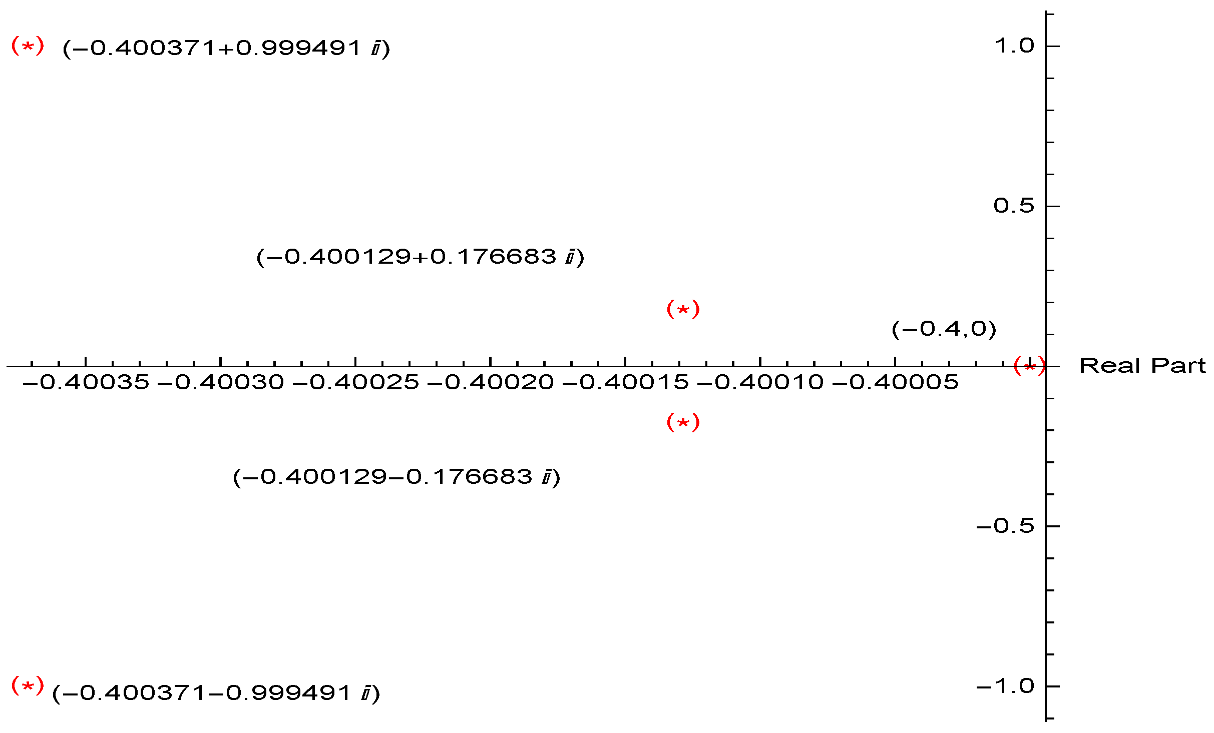
Also, at the initial values, instead of the DFE, we have the characteristic polynomial $-{\lambda }^5-2.001{\lambda }^4-2.6318{\lambda }^3-1.87748{\lambda }^2-0.654161\lambda -0.0887172$ and the eigenvalues given by

$${\lambda }_1=-0.400371+i0.999491,$$

$${\lambda }_2=-0.400371-i0.999491$$

$${\lambda }_3=-0.400129+i0.176683$$

$${\lambda }_4=-0.400129-i0.176683$$

$${\lambda }_5=-0.4.$$

Hence, as all the eigenvalues have negative real portions even at the initial values, the solutions of (5) created with the starting population count are locally asymptotically stable, as also shown in Figure 2.

4.4. Existence of Non-Negativity of Solutions

We are aware that the system (5) will undoubtedly have non-negative solutions if the system (1) does. Let us use a theorem to prove this.

Theorem 2.

Let $S\left(t\right),E\left(t\right),I\left(t\right),Q\left(t\right), and R\left(t\right)$ be the solutions of the system (1), as well as for the system (5), and they will be positive when expressed in the form of an exponential function.

Verification 2.

Since any solution of (1) is also a solution of (5), we shall consider (1) for our proof.

The solutions of our considered epidemic model (1) are as follows:

We treat each equation separately, using separation of variables for homogeneous equations and an integrating factor for the non-homogeneous R-equation.

1.

Generic homogeneous linear equation:

If $x^{\prime }\left(t\right)=\alpha \left(t\right)x\left(t\right)$ with $x\left(0\right)=x_0$, then

$${\displaystyle \frac{x^{\prime }\left(t\right)}{x\left(t\right)}}=\alpha \left(t\right)\Rightarrow ln{\displaystyle \frac{x\left(t\right)}{x_0}}={\int }_0^t\alpha \left(s\right)ds,$$

so

$$x\left(t\right)=x_{0}exp\left({\int }_0^t\alpha \left(s\right)ds\right).$$

2.

Solution for $S\left(t\right)$:

The $S\left(t\right)$-equation is

$$S^{\prime }\left(t\right)=-\left(aE\left(t\right)+v\right)S\left(t\right),$$

which is of the form $x^{\prime }\left(t\right)=\alpha \left(t\right)x$ with $\alpha \left(t\right)=-\left(aE\left(t\right)+v\right)$. Hence

$$S\left(t\right)=S_{0}exp\left(-{\int }_0^t\left(aE\left(s\right)+v\right)ds\right).$$

3.

Solution for $E\left(t\right)$:

The E-equation is

$$E^{\prime }\left(t\right)=\left(aS\left(t\right)-bI\left(t\right)-v\right)E\left(t\right),$$

so $\alpha \left(t\right)=aS\left(t\right)-bI\left(t\right)-v$ and

$$E\left(t\right)=E_{0}exp\left({\int }_0^t\left(aS\left(s\right)-bI\left(s\right)-v\right)ds\right).$$

4.

Solution for $I\left(t\right)$:

The I-equation is

$$I^{\prime }\left(t\right)=\left(bE\left(t\right)-cQ\left(t\right)-k-v\right)I,$$

so $\alpha \left(t\right)=bE\left(t\right)-cQ\left(t\right)-k-v$ and

$$I\left(t\right)=I_{0}exp\left({\int }_0^t\left(bE\left(s\right)-cQ\left(s\right)-k-v\right)ds\right).$$

5.

Solution for $Q\left(t\right)$:

The $Q\left(t\right)$-equation is

$$Q^{\prime }\left(t\right)=\left(cI\left(t\right)-uR\left(t\right)-v\right)Q\left(t\right),$$

so $\alpha \left(t\right)=cI\left(t\right)-uR\left(t\right)-v$ and

$$Q\left(t\right)=Q_{0}exp\left({\int }_0^t\left(cI\left(s\right)-uR\left(s\right)-v\right)ds\right).$$

6.

Solution for $R\left(t\right)$ (integrating factor):

The R-equation is

$$R^{\prime }\left(t\right)=(uQ\left(t\right)-v)R\left(t\right)+kI\left(t\right).$$

Write it in linear standard form

$$R^{\prime }\left(t\right)-(uQ\left(t\right)-v)R\left(t\right)=kI\left(t\right).$$

The integrating factor is

$$\mathrm{IF}\left(t\right)=exp\left(-{\int }_0^t\left(uQ\left(s\right)-v\right)ds\right).$$

Multiplying the linear equation by $\mathrm{IF}\left(t\right)$ gives

$${\displaystyle \frac{d}{dt}}\left(\mathrm{IF}\left(t\right)R\left(t\right)\right)=\mathrm{IF}\left(t\right)kI\left(t\right).$$

Integrating from 0 to t and using $\mathrm{IF}\left(0\right)=1$ yields

$$\mathrm{IF}\left(t\right)R\left(t\right)=R_0+k{\int }_0^t\mathrm{IF}\left(s\right)I\left(s\right)ds.$$

Therefore

$$R\left(t\right)=exp\left({\int }_0^t(uQ\left(s\right)-v)ds\right)\left[R_0+k{\int }_0^{t}exp\left(-{\int }_0^s(uQ\left(\tau \right)-v)d\tau \right)I\left(s\right)ds\right].$$

7.

Collected system (implicit):

Collecting the results, we obtain the implicit exponential representations:

$$\begin{array}{cc}\hfill S\left(t\right)& =S_{0}exp\left(-{\int }_0^t\left(aE\left(s\right)+v\right)ds\right);\hfill \\ \hfill E\left(t\right)& =E_{0}exp\left({\int }_0^t\left(aS\left(s\right)-bI\left(s\right)-v\right)ds\right);\hfill \\ \hfill I\left(t\right)& =I_{0}exp\left({\int }_0^t\left(bE\left(s\right)-cQ\left(s\right)-k-v\right)ds\right);\hfill \\ \hfill Q\left(t\right)& =Q_{0}exp\left({\int }_0^t\left(cI\left(s\right)-uR\left(s\right)-v\right)ds\right);\hfill \\ \hfill R\left(t\right)& =exp\left({\int }_0^t(uQ\left(s\right)-v)ds\right)\left[R_0+k{\int }_0^{t}exp\left(-{\int }_0^s(uQ\left(\tau \right)-v)d\tau \right)I\left(s\right)ds\right].\hfill \end{array}$$

8.

Remark

These formulas are implicit: each exponential contains integrals of other unknowns (the system is coupled). They are exact representations, but to obtain explicit time-functions, one must solve the coupled system (e.g., numerically) or find special reductions that decouple the equations.

The epidemic dynamics of the baseline SEIQR model in the ODE case (${\alpha }_i=1$) are presented in Figure 3. The curves exhibit the expected outbreak pattern, with rapid growth of exposed and infected individuals followed by decline as quarantine and recovery dominate. This provides a benchmark for comparison with fractional-order dynamics.

There will now be two scenarios in our analysis, based on the exponential term’s powers $t\to \infty$:

Case 1: Positive exponential terms: After integrating and multiplying by the prefix’s negative sign, if the power of e is positive, $(S,E,I,Q,R)\to \infty$ as $t\to \infty$.

Case 2: Negative exponential terms: After integrating and multiplying by the negative sign on the prefix, if the power of e is negative, then $(S,E,I,Q,R)\to 0$ as $t\to \infty$.

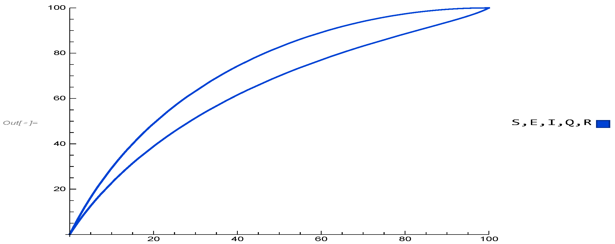
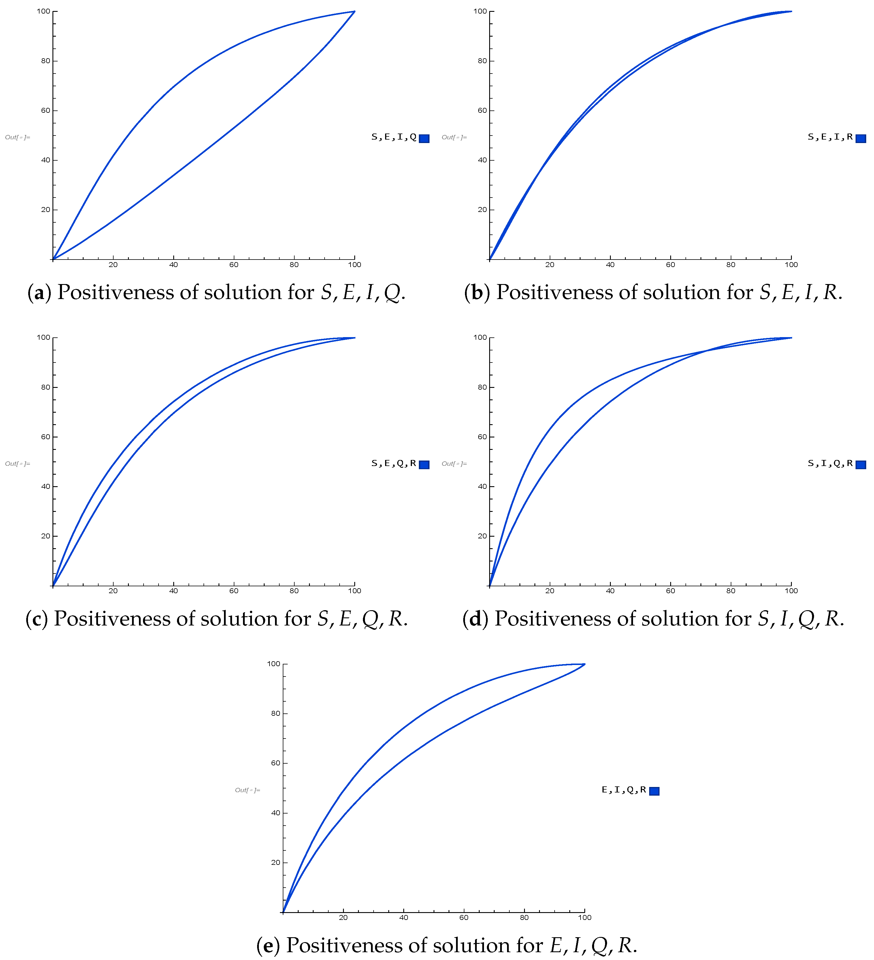
It is evident from both scenarios that $S,E,I,Q,R$ are non-negative; that is, $(S,E,I,Q,R)\ge 0$. Figure 4 and Figure 5 also support this assertion.

Additionally, the following lists the positiveness of the solutions for various permutations of the Figure 5 solutions:

As a result, only non-negative solutions in (1) exist, proving the positivity of (5) solutions.

5. Simulative Outcomes

The computer simulations of the standard and fractional-ordered SEIQR models obtained by using Mathematica are shown in this section. Using the Laplace Adomian Decomposition method (LADM), numerical simulations are obtained. It is recommended that readers read [13].

Laplace Adomian Decomposition (LADM) Solutions

The noninteger model (5) is taken into consideration in this instance, and the LADM is used to simulate the findings.

$$L^{-1}\left(-{\displaystyle \frac{v}{s^{{\alpha }_1}}}L\left(S_A\right)-{\displaystyle \frac{a}{s^{{\alpha }_1}}}L\left(W_A\right)\right)=S\left(A+1\right),$$

$$L^{-1}\left(-{\displaystyle \frac{b}{s^{{\alpha }_2}}}L\left(X_A\right)-{\displaystyle \frac{a}{s^{{\alpha }_2}}}L\left(W_A\right)-{\displaystyle \frac{v}{s^{{\alpha }_2}}}L\left(E_A\right)\right)=E\left(A+1\right),$$

$$L^{-1}\left(-{\displaystyle \frac{k}{s^{{\alpha }_3}}}L\left(I_A\right)+{\displaystyle \frac{b}{s^{{\alpha }_3}}}L\left(X_A\right)-{\displaystyle \frac{c}{s^{{\alpha }_3}}}L\left(Y_A\right)-{\displaystyle \frac{v}{s^{{\alpha }_3}}}L\left(I_A\right)\right)=I\left(A+1\right),$$

$$L^{-1}\left({\displaystyle \frac{c}{s^{{\alpha }_4}}}L\left(Y_A\right)-{\displaystyle \frac{v}{s^{{\alpha }_4}}}L\left(Q_A\right)-{\displaystyle \frac{u}{s^{{\alpha }_4}}}L\left(Z_A\right)\right)=Q\left(A+1\right),$$

$$L^{-1}\left({\displaystyle \frac{u}{s^{{\alpha }_5}}}L\left(Z_A\right)-{\displaystyle \frac{v}{s^{{\alpha }_5}}}L\left(R_A\right)+{\displaystyle \frac{k}{s^{{\alpha }_5}}}L\left(I_A\right)\right)=R\left(A+1\right).$$

where $\left(W_A,X_A,Y_A,Z_A\right)$ are Adomian polynomials defined by

$$W_A={\displaystyle \frac{1}{A!}}{\displaystyle \frac{d^A}{d{\lambda }^A}}\sum _{l=0}^A\left({\lambda }^l{S}_l.{\lambda }^l{E}_l\right)|\lambda =0,$$

$$X_A={\displaystyle \frac{1}{A!}}{\displaystyle \frac{d^A}{d{\lambda }^A}}\sum _{l=0}^A\left({\lambda }^l{E}_l.{\lambda }^l{I}_l\right)|\lambda =0,$$

$$Y_A={\displaystyle \frac{1}{A!}}{\displaystyle \frac{d^A}{d{\lambda }^A}}\sum _{l=0}^A\left({\lambda }^l{I}_l.{\lambda }^l{Q}_l\right)|\lambda =0,$$

$$Z_A={\displaystyle \frac{1}{A!}}{\displaystyle \frac{d^A}{d{\lambda }^A}}\sum _{l=0}^A\left({\lambda }^l{Q}_l.{\lambda }^l{R}_l\right)|\lambda =0.$$

Also,

$$S\left(t\right)=\sum _{A=0}^{\infty }S\left(A\right),E\left(t\right)=\sum _{A=0}^{\infty }E\left(A\right),$$

$$I\left(t\right)=\sum _{A=0}^{\infty }I\left(A\right),\left(t\right)=\sum _{A=0}^{\infty }Q\left(A\right),$$

$$R\left(t\right)=\sum _{A=0}^{\infty }R\left(A\right).$$

For model (5), after assigning the values to all the parameters, the solution obtained by LADM up to order 4 defined for ${\alpha }_1={\alpha }_2={\alpha }_3={\alpha }_4={\alpha }_5=1$ is found.

The equations below give the solutions of fractional S, E, I, Q, R at the order $0\le {\alpha }_i\le 1.$

Suceptible solutions are given by

$$\begin{array}{cc}At{\alpha }_1=0\hfill & 37.137,\hfill \\ At{\alpha }_1=0.1\hfill & 100-136.648t^{0.1}+164.458t^{0.2}-93.0663t^{0.3},\hfill \\ At{\alpha }_1=0.2\hfill & 100-141.586t^{0.2}+170.186t^{0.4}-92.4834t^{0.6},\hfill \\ At{\alpha }_1=0.3\hfill & 100-144.852t^{0.3}+168.995t^{0.6}-84.5368t^{0.9},\hfill \\ At{\alpha }_1=0.4\hfill & 100-146.518t^{0.4}+162.124t^{0.8}-72.2256t^{1.2},\hfill \\ At{\alpha }_1=0.5\hfill & 100-146.689t^{0.5}+151.t^{1.0}-58.2764t^{1.5},\hfill \\ At{\alpha }_1=0.6\hfill & 100-145.493t^{0.6}+137.048t^{1.2}-44.7181t^{1.8},\hfill \\ At{\alpha }_1=0.7\hfill & 100-143.071t^{0.7}+121.562t^{1.4}-32.7887t^{2.1},\hfill \\ At{\alpha }_1=0.8\hfill & 100-139.577t^{0.8}+105.622t^{1.6}-23.0441t^{2.4},\hfill \\ At{\alpha }_1=0.9\hfill & 100-135.168t^{0.9}+90.0691t^{1.8}-15.5496t^{2.7},\hfill \\ At{\alpha }_1=1.0\hfill & 100-130.t+75.5t^2-10.0772t^3.\hfill \end{array}$$

(10)

Exposed solutions are given by

$$\begin{array}{cc}At{\alpha }_2=0\hfill & 93.4699,\hfill \\ At{\alpha }_2=0.1\hfill & 100+21.0227t^{0.1}-107.747t^{0.2}+80.3391t^{0.3},\hfill \\ At{\alpha }_2=0.2\hfill & 100+21.7825t^{0.2}-111.5t^{0.4}+79.8194t^{0.6},\hfill \\ At{\alpha }_2=0.3\hfill & 100+22.2849t^{0.3}-110.72t^{0.6}+72.9379t^{0.9},\hfill \\ At{\alpha }_2=0.4\hfill & 100+22.5412t^{0.4}-106.218t^{0.8}+62.2893t^{1.2},\hfill \\ At{\alpha }_2=0.5\hfill & 100+22.5676t^{0.5}-98.93t^{1.0}+50.2317t^{1.5},\hfill \\ At{\alpha }_2=0.6\hfill & 100+22.3835t^{0.6}-89.7892t^{1.2}+38.5185t^{1.8},\hfill \\ At{\alpha }_2=0.7\hfill & 100+22.0109t^{0.7}-79.6429t^{1.4}+28.2186t^{2.1},\hfill \\ At{\alpha }_2=0.8\hfill & 100+21.4734t^{0.8}-69.2t^{1.6}+19.8106t^{2.4},\hfill \\ At{\alpha }_2=0.9\hfill & 100+20.7951t^{0.9}-59.0102t^{1.8}+13.3493t^{2.7},\hfill \\ At{\alpha }_2=1.0\hfill & 100+20.t-49.465t^2+8.63566t^3.\hfill \end{array}$$

(11)

Infected solutions are given by

$$\begin{array}{cc}At{\alpha }_3=0\hfill & 185.34,\hfill \\ At{\alpha }_3=0.1\hfill & 100-21.1279t^{0.1}+35.9848t^{0.2}+80.3391t^{0.3},\hfill \\ At{\alpha }_3=0.2\hfill & 100-21.8914t^{0.2}+37.2382t^{0.4}+79.8194t^{0.6},\hfill \\ At{\alpha }_3=0.3\hfill & 100-22.3963t^{0.3}+36.9777t^{0.6}+72.9379t^{0.9},\hfill \\ At{\alpha }_3=0.4\hfill & 100-22.6539t^{0.4}+35.4742t^{0.8}+62.2893t^{1.2},\hfill \\ At{\alpha }_3=0.5\hfill & 100-22.6804t^{0.5}+33.0401t^1+50.2317t^{1.5},\hfill \\ At{\alpha }_3=0.6\hfill & 100-22.4954t^{0.6}+29.9873t^{1.2}+38.5185t^{1.8},\hfill \\ At{\alpha }_3=0.7\hfill & 100-22.121t^{0.7}+26.5987t^{1.4}+28.2186t^{2.1},\hfill \\ At{\alpha }_3=0.8\hfill & 100-21.5808t^{0.8}+23.111t^{1.6}+19.8106t^{2.4},\hfill \\ At{\alpha }_3=0.9\hfill & 100-20.8991t^{0.9}+19.7079t^{1.8}+13.3493t^{2.7},\hfill \\ At{\alpha }_3=1\hfill & 100-20.1t+16.5201t^2+8.63566t^3.\hfill \end{array}$$

(12)

Quarantined solutions are given by

$$\begin{array}{cc}At{\alpha }_4=0\hfill & 44.6471,\hfill \\ At{\alpha }_4=0.1\hfill & 100-31.5341t^{0.1}+26.041t^{0.2}-54.9231t^{0.3},\hfill \\ At{\alpha }_4=0.2\hfill & 100-32.6737t^{0.2}+26.948t^{0.4}-55.2511t^{0.6},\hfill \\ At{\alpha }_4=0.3\hfill & =100-33.4273t^{0.3}+26.7595t^{0.6}-51.4484t^{0.9},\hfill \\ At{\alpha }_3=0.4\hfill & 100-33.8118t^{0.4}+25.6715t^{0.8}-45.0432t^{1.2},\hfill \\ At{\alpha }_4=0.5\hfill & 100-33.8514t^{0.5}+23.91t^1-37.4688t^{1.5},\hfill \\ At{\alpha }_4=0.6\hfill & 100-33.5752t^{0.6}+21.7008t^{1.2}-29.8375t^{1.8},\hfill \\ At{\alpha }_3=0.7\hfill & 100-33.0164t^{0.7}+19.2486t^{1.4}-22.8752t^{2.1},\hfill \\ At{\alpha }_4=0.8\hfill & 100-32.2101t^{0.8}+16.7247t^{1.6}-16.9588t^{2.4},\hfill \\ At{\alpha }_4=0.9\hfill & 100-31.1926t^{0.9}+14.2619t^{1.8}-12.201t^{2.7},\hfill \\ At{\alpha }_4=1\hfill & 100-30.t+11.955t^2-8.54349t^3.\hfill \end{array}$$

(13)

Recovered solutions are given by

$$\begin{array}{cc}At{\alpha }_5=0\hfill & 97.6649,\hfill \\ At{\alpha }_5=0.1\hfill & 100+0.105114t^{0.1}-13.0914t^{0.2}+10.6799t^{0.3},\hfill \\ At{\alpha }_5=0.2\hfill & 100+0.108912t^{0.2}-13.5474t^{0.4}+10.7266t^{0.6},\hfill \\ At{\alpha }_5=0.3\hfill & 100+0.111424t^{0.3}-13.4526t^{0.6}+9.96472t^{0.9},\hfill \\ At{\alpha }_5=0.4\hfill & 100+0.112706t^{0.4}-12.9056t^{0.8}+8.69742t^{1.2},\hfill \\ At{\alpha }_5=0.5\hfill & 100+0.112838t^{0.5}-12.0201t^1+7.20791t^{1.5},\hfill \\ At{\alpha }_5=0.6\hfill & 100+0.111917t^{0.6}-10.9095t^{1.2}+5.7146t^{1.8},\hfill \\ At{\alpha }_5=0.7\hfill & 100+0.110055t^{0.7}-9.6767t^{1.4}+4.3588t^{2.1},\hfill \\ At{\alpha }_5=0.8\hfill & 100+0.107367t^{0.8}-8.40787t^{1.6}+3.21255t^{2.4},\hfill \\ At{\alpha }_5=0.9\hfill & 100+0.103975t^{0.9}-7.1698t^{1.8}+2.29587t^{2.7},\hfill \\ At{\alpha }_5=1.0\hfill & 100+0.1t-6.01005t^2+1.59551t^3.\hfill \end{array}$$

(14)

Now, for $1\le {\alpha }_i\le 2$, the fractional SEIQR solutions are presented below:

$$\begin{array}{cc}At{\alpha }_1=1\hfill & 100-130.t+75.5t^2-10.0772t^3,\hfill \\ At{\alpha }_1=1.1\hfill & 100-124.225t^{1.1}+62.2946t^{2.2}-6.26395t^{3.3},\hfill \\ At{\alpha }_1=1.2\hfill & 100-117.988t^{1.2}+50.6506t^{2.4}-3.7215t^{3.6},\hfill \\ At{\alpha }_1=1.3\hfill & 100-111.424t^{1.3}+40.6239t^{2.6}-2.09826t^{3.9},\hfill \\ At{\alpha }_1=1.4\hfill & 100-104.656t^{1.4}+32.1675t^{2.8}-1.10731t^{4.2},\hfill \\ At{\alpha }_1=1.5\hfill & 100-97.7929t^{1.5}+25.1667t^3-0.53136t^{4.5},\hfill \\ At{\alpha }_1=1.6\hfill & 100-90.933t^{1.6}+19.4671t^{3.2}-0.21555t^{4.8},\hfill \\ At{\alpha }_1=1.7\hfill & 100-84.1595t^{1.7}+14.8972t^{3.4}-0.0551653t^{5.1},\hfill \\ At{\alpha }_1=1.8\hfill & 100-77.5429t^{1.8}+11.2844t^{3.6}+0.0172057t^{5.4},\hfill \\ At{\alpha }_1=1.9\hfill & 100-71.1411t^{1.9}+8.46514t^{3.8}+0.0429063t^{5.7},\hfill \\ At{\alpha }_1=2\hfill & 100-65.t^2+6.29167t^4+0.0460236t^6.\hfill \end{array}$$

(15)

$$\begin{array}{cc}At{\alpha }_2=1\hfill & 100+20.t-49.465t^2+8.63566t^3,\hfill \\ At{\alpha }_2=1.1\hfill & 100+19.1116t^{1.1}-40.8133t^{2.2}+5.35506t^{3.3},\hfill \\ At{\alpha }_2=1.2\hfill & 100+18.1521t^{1.2}-33.1846t^{2.4}+3.17098t^{3.6},\hfill \\ At{\alpha }_2=1.3\hfill & 100+17.1422t^{1.3}-26.6154t^{2.6}+1.77925t^{3.9},\hfill \\ At{\alpha }_2=1.4\hfill & 100+16.1009t^{1.4}-21.0751t^{2.8}+0.931846t^{4.2},\hfill \\ At{\alpha }_2=1.5\hfill & 100+15.0451t^{1.5}-16.4883t^3+0.441134t^{4.5},\hfill \\ At{\alpha }_2=1.6\hfill & 100+13.9897t^{1.6}-12.7542t^{3.2}+0.173535t^{4.8},\hfill \\ At{\alpha }_2=1.7\hfill & 100+12.9476t^{1.7}-9.76016t^{3.4}+0.0388578t^{5.1},\hfill \\ At{\alpha }_2=1.8\hfill & 100+11.9297t^{1.8}-7.39316t^{3.6}-0.0208584t^{5.4},\hfill \\ At{\alpha }_2=1.9\hfill & 100+10.9448t^{1.9}-5.54607t^{3.8}-0.0410798t^{5.7},\hfill \\ At{\alpha }_2=2\hfill & 100+10.t^2-4.12208t^4-0.0424029t^6.\hfill \end{array}$$

(16)

$$\begin{array}{cc}At{\alpha }_3=1\hfill & 100-20.1t+16.5201t^2+8.63566t^3,\hfill \\ At{\alpha }_3=1.1\hfill & 100-19.2071t^{1.1}+13.6306t^{2.2}+5.35506t^{3.3},\hfill \\ At{\alpha }_3=1.2\hfill & 100-18.2428t^{1.2}+11.0828t^{2.4}+3.17098t^{3.6},\hfill \\ At{\alpha }_3=1.3\hfill & 100-17.2279t^{1.3}+8.88886t^{2.6}+1.77925t^{3.9},\hfill \\ At{\alpha }_3=1.4\hfill & 100-16.1814t^{1.4}+7.03853t^{2.8}+0.931846t^{4.2},\hfill \\ At{\alpha }_3=1.5\hfill & 100-15.1203t^{1.5}+5.50668t^3+0.441134t^{4.5},\hfill \\ At{\alpha }_3=1.6\hfill & 100-14.0596t^{1.6}+4.25956t^{3.2}+0.173535t^{4.8},\hfill \\ At{\alpha }_3=1.7\hfill & 100-13.0124t^{1.7}+3.25965t^{3.4}+0.0388578t^{5.1},\hfill \\ At{\alpha }_3=1.8\hfill & 100-11.9893t^{1.8}+2.46913t^{3.6}-0.0208584t^{5.4},\hfill \\ At{\alpha }_3=1.9\hfill & 100-10.9995t^{1.9}+1.85225t^{3.8}-0.0410798t^{5.7},\hfill \\ At{\alpha }_3=2\hfill & 100-10.05t^2+1.37667t^4-0.0424029t^6.\hfill \end{array}$$

(17)

$$\begin{array}{cc}At{\alpha }_4=1\hfill & 100-30.t+11.955t^2-8.54349t^3,\hfill \\ At{\alpha }_4=1.1\hfill & 100-28.6674t^{1.1}+9.864t^{2.2}-5.83685t^{3.3},\hfill \\ At{\alpha }_4=1.2\hfill & 100-27.2281t^{1.2}+8.02024t^{2.4}-3.89884t^{3.6},\hfill \\ At{\alpha }_4=1.3\hfill & 100-25.7133t^{1.3}+6.43257t^{2.6}-2.55092t^{3.9},\hfill \\ At{\alpha }_4=1.4\hfill & 100-24.1513t^{1.4}+5.09355t^{2.8}-1.6374t^{4.2},\hfill \\ At{\alpha }_4=1.5\hfill & 100-22.5676t^{1.5}+3.985t^3-1.03259t^{4.5},\hfill \\ At{\alpha }_4=1.6\hfill & 100-20.9845t^{1.6}+3.0825t^{3.2}-0.640581t^{4.8},\hfill \\ At{\alpha }_4=1.7\hfill & 100-19.4214t^{1.7}+2.3589t^{3.4}-0.391378t^{5.1},\hfill \\ At{\alpha }_4=1.8\hfill & 100-17.8945t^{1.8}+1.78682t^{3.6}-0.235753t^{5.4},\hfill \\ At{\alpha }_4=1.9\hfill & 100-16.4172t^{1.9}+1.34041t^{3.8}-0.140148t^{5.7},\hfill \\ At{\alpha }_4=2\hfill & 100-15.t^2+0.99625t^4-0.0822957t^6.\hfill \end{array}$$

(18)

$$\begin{array}{cc}At{\alpha }_5=1\hfill & 100+0.1t-6.01005t^2+1.59551t^3,\hfill \\ At{\alpha }_5=1.1\hfill & 100+0.0955579t^{1.1}-4.95886t^{2.2}+1.08076t^{3.3},\hfill \\ At{\alpha }_5=1.2\hfill & 100+0.0907604t^{1.2}-4.03196t^{2.4}+0.714996t^{3.6},\hfill \\ At{\alpha }_5=1.3\hfill & 100+0.085711t^{1.3}-3.2338t^{2.6}+0.462771t^{3.9},\hfill \\ At{\alpha }_5=1.4\hfill & 100+0.0805043t^{1.4}-2.56064t^{2.8}+0.293465t^{4.2},\hfill \\ At{\alpha }_5=1.5\hfill & 100+0.0752253t^{1.5}-2.00335t^3+0.182571t^{4.5},\hfill \\ At{\alpha }_5=1.6\hfill & 100+0.0699484t^{1.6}-1.54964t^{3.2}+0.111555t^{4.8},\hfill \\ At{\alpha }_5=1.7\hfill & 100+0.0647381t^{1.7}-1.18587t^{3.4}+0.0670125t^{5.1},\hfill \\ At{\alpha }_5=1.8\hfill & 100+0.0596484t^{1.8}-0.898277t^{3.6}+0.039612t^{5.4},\hfill \\ At{\alpha }_5=1.9\hfill & 100+0.0547239t^{1.9}-0.673853t^{3.8}+0.0230594t^{5.7},\hfill \\ At{\alpha }_5=2\hfill & 100+0.05t^2-0.500838t^4+0.0132292t^6.\hfill \end{array}$$

(19)

6. Results and Discussion

In this study, we developed and analyzed a fuzzy fractional-order SEIQR model to capture epidemic dynamics with both non-integer rate of changes and uncertainty. This classical framework served as the foundation for the fractional and fuzzy extensions presented in this work.

The stability properties of the system were investigated using eigenvalue analysis. Figure 2 displays the real and imaginary parts of the eigenvalues, confirming the local asymptotic stability of the initial populations as in Remark 2 of Theorem 1, and in Theorem 1, the local asymptotic stability of IFE points is confirmed. This implies that, under appropriate parameter conditions, the infection will vanish over time. The biological validity of the model was also verified through positivity results (Theorem 2). As shown in Figure 4 and Figure 5, all compartmental populations remain non-negative for both individual classes and their combinations, thereby ensuring feasibility of the framework.

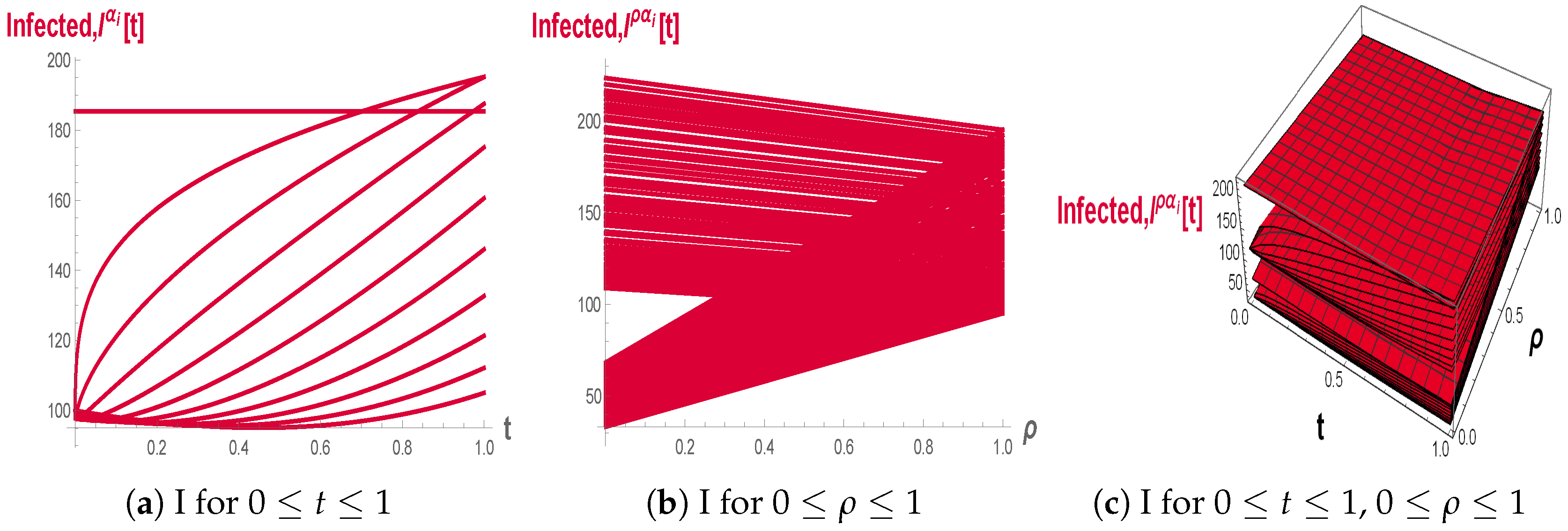
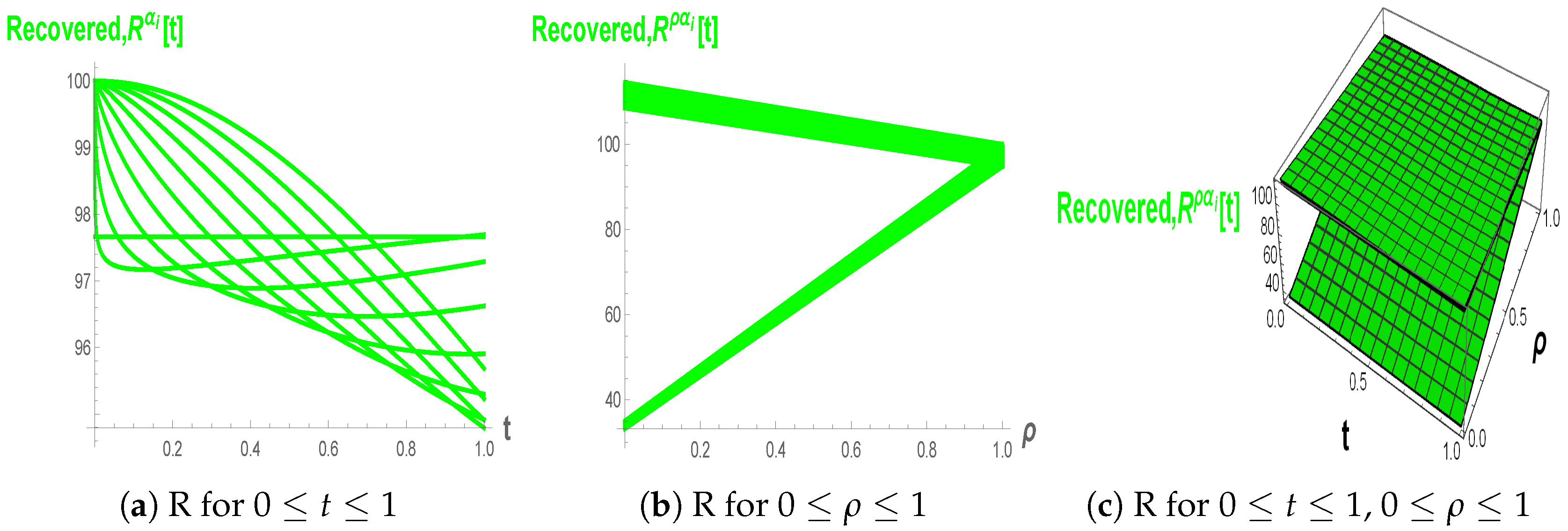
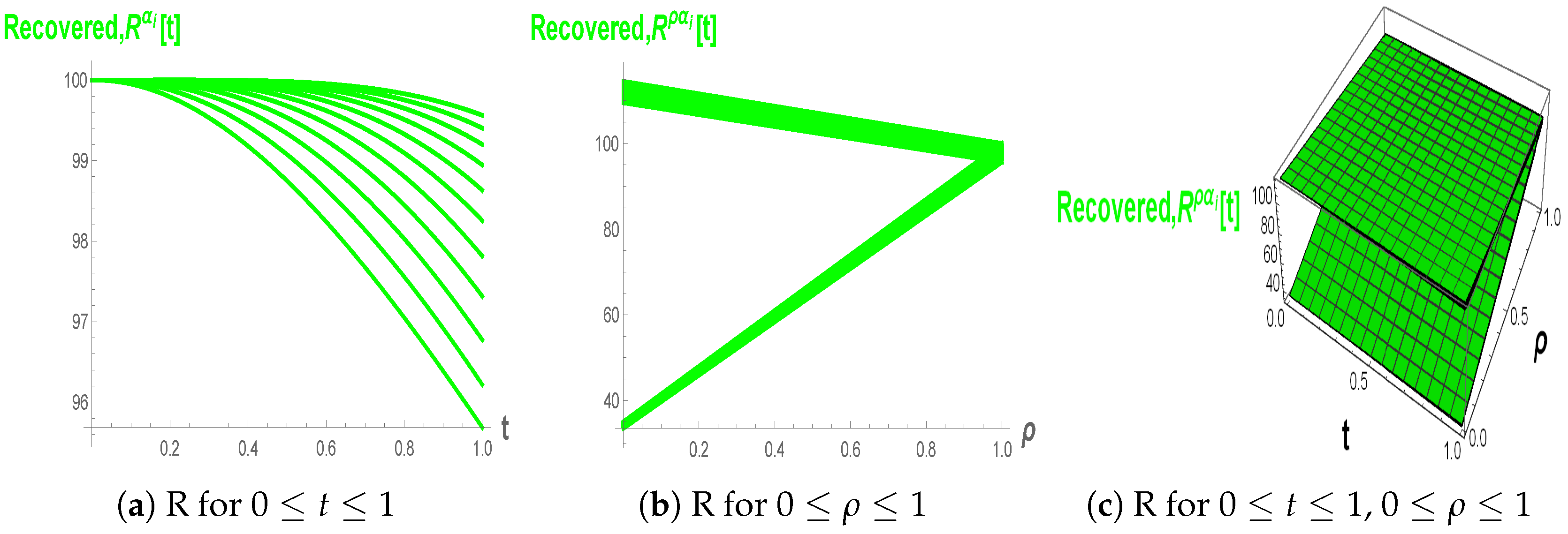
The fractional-order SEIQR epidemic model results are depicted in Figure 6a–c, Figure 7a–c, Figure 8a–c, Figure 9a–c, Figure 10a–c, Figure 11a–c, Figure 12a–c, Figure 13a–c, Figure 14a–c and Figure 15a–c. For each compartment ($S,E,I,Q,R$), the figures labeled “a” show fractional-order dynamics over $0\le t\le 1$ and $0\le {\alpha }_i\le 1$, while those labeled “b” and “c” display fuzzy fractional cases two-dimensionally (2D) and three-dimensionally (3D) for both $0\le {\alpha }_i\le 1$ and $1\le {\alpha }_i\le 2$, and $0\le \rho \le 1$. The 2D plots are obtained by deriving the expression for both $0\le {\alpha }_i\le 1$ or $1\le {\alpha }_i\le 2$ and $0\le t\le 1$ and later varying these solutions for various $0\le \rho \le 1$, whereas the 3D plots are carried out by deriving the expression for $0\le {\alpha }_i\le 1$ or $1\le {\alpha }_i\le 2$ and later varying these solutions for various $0\le t\le 1$ and $0\le \rho \le 1$.

Unlike their integer-order counterparts, the fractional solutions exhibit slower decay of infections, reflecting memory effects and persistent epidemic activity. Increasing the fractional order ($1\le {\alpha }_i\le 2$), as in Figure 11a–c, Figure 12a–c, Figure 13a–c, Figure 14a–c and Figure 15a–c, leads to quicker stabilization, demonstrating the flexible behavior enabled by fractional calculus.

The fuzzy fractional extensions, documented in Figure 6b, Figure 7b, Figure 8b, Figure 9b, Figure 10b, Figure 11b, Figure 12b, Figure 13b, Figure 14b and Figure 15b and Figure 6c, Figure 7c, Figure 8c, Figure 9c, Figure 10c, Figure 11c, Figure 12c, Figure 13c, Figure 14c and Figure 15c, capture parameter uncertainties. These figures show broad families of possible epidemic trajectories arising from variations in transmission and recovery rates. This integration of fuzziness yields a more comprehensive depiction of outcome ranges compared to deterministic models.

In particular, for $0\le {\alpha }_i\le 1$, Figure 6a–c show that the Susceptible population $S^{\rho }\left(t\right)$ decreases monotonically over time, with smaller fractional orders producing a slower decay and hence a longer persistence of susceptibility in the population. The 2D and 3D fuzzy plots further indicate that as the fuzziness level $\rho$ varies in $[0,1]$, the curves form a band of possible trajectories, reflecting uncertainty in the effective contact rate and illustrating a range of feasible epidemic paths for $S\left(t\right)$. Figure 7a–c illustrate that the Exposed population initially increases to a peak and then declines, and that lower values of ${\alpha }_i$ delay this peak and stretch the tail of $E^{\rho }\left(t\right)$, evidencing the memory effect of the fractional operator. The fuzzy representations in panels (b) and (c) show how varying $\rho$ generates a family of exposed trajectories, capturing uncertainty in progression from susceptibility to exposure.

In Figure 8a–c, the Infected population exhibits a gradual rise followed by a slower decay when $0\le {\alpha }_i\le 1$, with smaller fractional orders leading to more persistent infection levels compared to higher orders. The fuzzy 2D and 3D plots demonstrate that changes in $\rho$ widen the envelope of $I^{\rho }\left(t\right)$ trajectories, indicating that uncertainty in transmission and removal rates can substantially modify both the peak size and duration of the infectious phase. Figure 9a–c show that the Quarantined population decreases over time for all fractional orders in $[0,1]$, with lower ${\alpha }_i$ again producing a slower decay, which can be interpreted as a longer retention of individuals in quarantine under stronger memory effects. The fuzzy plots reveal a sheet of plausible $Q^{\rho }\left(t\right)$ curves over $\rho \in [0,1]$, quantifying how parameter uncertainty influences the rate at which quarantine measures reduce the isolated population. As displayed in Figure 10a–c, the Recovered population increases with time and approaches a plateau, and smaller fractional orders yield a more gradual growth, indicating that memory slows the accumulation of recovered individuals. The fuzzy fractional views in (b) and (c) show triangular–shaped bands in $\rho$–space, highlighting that uncertainty in recovery-related parameters generates a continuum of possible recovery curves around the nominal trajectory.

For $1\le {\alpha }_i\le 2$, Figure 11a–c show that the Susceptible population $S^{\rho }\left(t\right)$ decays more rapidly than in the case $0\le {\alpha }_i\le 1$, indicating that higher fractional orders reduce the memory effect and drive the system closer to classical first–order dynamics. The fuzzy 2D and 3D plots in panels (b) and (c) reveal that, although variation of $\rho$ still generates a band of admissible trajectories, the overall spread is narrower and the population stabilizes faster, reflecting reduced sensitivity to parameter uncertainty in this regime. Figure 12a–c illustrate that, for $1\le {\alpha }_i\le 2$, the Exposed population $E^{\rho }\left(t\right)$ exhibits a shorter transient phase, with faster departure from the initial level and earlier decline compared to the lower–order case. The fuzzy surfaces show that increasing ${\alpha }_i$ compresses the range of possible exposed trajectories over $\rho \in [0,1]$, suggesting that strong fractional effects attenuate the impact of uncertainty on the exposure dynamics. As seen in Figure 13a–c, when $1\le {\alpha }_i\le 2$ the Infected population $I^{\rho }\left(t\right)$ reaches lower peaks and returns more quickly towards baseline, demonstrating that higher fractional orders enhance the effective removal of infection. The fuzzy 2D and 3D plots indicate that the family of infected trajectories over $\rho$ remains bounded within a relatively tight band, which means that in this parameter range the epidemic outcomes are less sensitive to moderate fluctuations in transmission and recovery rates. Figure 14a–c show that the Quarantined population $Q^{\rho }\left(t\right)$ decreases almost linearly in time for $1\le {\alpha }_i\le 2$, with little curvature compared to the sub-unitary orders, reflecting a more direct, non-memory-dominated decay of quarantined individuals. The fuzzy representations again form a relatively thin sheet over $\rho \in [0,1]$, which indicates that, under higher fractional orders, the quarantine dynamics are comparatively robust to uncertainty in the underlying parameters. In Figure 15a–c, the Recovered population $R^{\rho }\left(t\right)$ increases quickly and then saturates, and this saturation occurs earlier for $1\le {\alpha }_i\le 2$ than in the case of $0\le {\alpha }_i\le 1$, highlighting the accelerating effect of higher fractional orders on the build-up of immunity. The fuzzy 2D and 3D plots reveal that, although uncertainty in $\rho$ still generates a continuum of recovery curves, these trajectories cluster closely, showing that in the high-order regime, the long-term recovered level is only weakly affected by fuzziness in model parameters.

General model features such as formulation, equilibrium positivity, and stability supported by Figure 1, Figure 2, Figure 3, Figure 4 and Figure 5 confirm the robustness and utility of both fractional and fuzzy fractional SEIQR models.

From a computational perspective, the fourth-order LADM approach ensured the accuracy of fractional solutions. As $t\to \infty$, the solutions of both classical and fractional models remain positive (Theorem 2), while increasing the LADM order reduces the decay rate and improves approximation precision. A summary of simulations across different parameter values is provided in

Table 1. Summary of figures.

Figures	Label
Model Formulation	Figure 1
Real and Imaginary Parts of Eigenvalues	Figure 2
SEIQR Model Compartment Curves-1	Figure 3
Positiveness of Solutions for $S,E,I,Q,R$	Figure 4
Positiveness of Different Combinations of $S,E,I,Q,R$	Figure 5
Fractional Susceptible $0\le t\le 1$, $0\le {\alpha }_i\le 1$	Figure 6a
Fuzzy Fractional Susceptible-2D $0\le t\le 1$, $0\le {\alpha }_i\le 1$, $0\le \rho \le 1$	Figure 6b
Fuzzy Fractional Susceptible-3D $0\le t\le 1$, $0\le {\alpha }_i\le 1$, $0\le \rho \le 1$	Figure 6c
Fractional Exposed $0\le t\le 1$, $0\le {\alpha }_i\le 1$	Figure 7a
Fuzzy Fractional Exposed-2D $0\le t\le 1$, $0\le {\alpha }_i\le 1$, $0\le \rho \le 1$	Figure 7b
Fuzy Fractional Exposed-3D $0\le t\le 1$, $0\le {\alpha }_i\le 1$, $0\le \rho \le 1$	Figure 7c
Fractional Infected $0\le t\le 1$, $0\le {\alpha }_i\le 1$	Figure 8a
Fuzzy Fractional Infected-2D $0\le t\le 1$, $0\le {\alpha }_i\le 1$, $0\le \rho \le 1$	Figure 8b
Fuzzy Fractional Infected-3D $0\le t\le 1$, $0\le {\alpha }_i\le 1$, $0\le \rho \le 1$	Figure 8c
Fractional Quarantined $0\le t\le 1$, $0\le {\alpha }_i\le 1$	Figure 9a
Fuzzy Fractional Quarantined-2D $0\le t\le 1$, $0\le {\alpha }_i\le 1$, $0\le \rho \le 1$	Figure 9b
Fuzzy Fractional Quarantined-3D $0\le t\le 1$, $0\le {\alpha }_i\le 1$, $0\le \rho \le 1$	Figure 9c
Fractional Recovered $0\le t\le 1$, $0\le {\alpha }_i\le 1$	Figure 10a
Fuzzy Fractional Recovered-2D $0\le t\le 1$, $0\le {\alpha }_i\le 1$, $0\le \rho \le 1$	Figure 10b
Fuzzy Fractional Recovered-3D $0\le t\le 1$, $0\le {\alpha }_i\le 1$, $0\le \rho \le 1$	Figure 10c
Fractional Susceptible $0\le t\le 1$, $1\le {\alpha }_i\le 2$	Figure 11a
Fuzzy Fractional Susceptible-2D $0\le t\le 1$, $1\le {\alpha }_i\le 2$, $0\le \rho \le 1$	Figure 11b
Fuzzy Fractional Susceptible-3D $0\le t\le 1$, $1\le {\alpha }_i\le 2$, $0\le \rho \le 1$	Figure 11c
Fractional Exposed $0\le t\le 1$, $1\le {\alpha }_i\le 2$	Figure 12a
Fuzzy Fractional Exposed-2D $0\le t\le 1$, $1\le {\alpha }_i\le 2$, $0\le \rho \le 1$	Figure 12b
Fuzy Fractional Exposed-3D $0\le t\le 1$, $1\le {\alpha }_i\le 2$, $0\le \rho \le 1$	Figure 12c
Fractional Infected $0\le t\le 1$, $1\le {\alpha }_i\le 2$	Figure 13a
Fuzzy Fractional Infected-2D $0\le t\le 1$, $1\le {\alpha }_i\le 2$, $0\le \rho \le 1$	Figure 13b
Fuzzy Fractional Infected-3D $0\le t\le 1$, $1\le {\alpha }_i\le 2$, $0\le \rho \le 1$	Figure 13c
Fractional Quarantined $0\le t\le 1$, $1\le {\alpha }_i\le 2$	Figure 14a
Fuzzy Fractional Quarantined-2D $0\le t\le 1$, $1\le {\alpha }_i\le 2$, $0\le \rho \le 1$	Figure 14b
Fuzzy Fractional Quarantined-2D $0\le t\le 1$, $1\le {\alpha }_i\le 2$, $0\le \rho \le 1$	Figure 14c
Fractional Recovered $0\le t\le 1$, $1\le {\alpha }_i\le 2$	Figure 15a
Fuzzy Fractional Recovered-2D $0\le t\le 1$, $1\le {\alpha }_i\le 2$, $0\le \rho \le 1$	Figure 15b
Fuzzy Fractional Recovered-3D $0\le t\le 1$, $1\le {\alpha }_i\le 2$, $0\le \rho \le 1$	Figure 15c

.

In conclusion, the classical SEIQR model offers a useful baseline, but fractional derivatives enrich the dynamics by incorporating fractional effects ($\alpha$), and fuzzy logic adds robustness by addressing uncertainty ($\rho$). Together, these extensions provide a comprehensive and flexible framework for modeling epidemics. Beyond theoretical contributions, the model has practical applications in guiding vaccination strategies, quarantine measures, and adaptive policies to mitigate recurrent outbreaks. Future work will extend this framework to emerging variants, such as Omicron, further enhancing epidemic preparedness and management.

6.1. Key Findings

The investigation presents a fuzzy fractional SEIQR epidemic model, which can provide biologically meaningful solutions by the positivity, boundedness, and local asymptotic stability of the equilibrium if the parameters are chosen properly. The memory effects due to fractional-order dynamics can, depending on the order ${\alpha }_i$, either slow down or speed up the infection’s decay while the fuzzy extension parameterized by $\rho$ holds uncertainty in transmission and recovery, thus capturing not just one deterministic curve but families of plausible epidemic trajectories. The numerical experiments, which are based on the LADM scheme of the fourth order, not only verify the theoretical results but also showcase the model’s adaptability to represent various epidemic scenarios within one unified structure.

6.2. Limitations and Future Prospects

The current model presumes perfect mixing of the populations, constant parameters, and does not consider spatial heterogeneity, age structure, stochastic effects, or optimal control interventions. To add on, the parameter sets used in the simulations are merely illustrative and not fitted to the data; hence, direct quantitative prediction for specific diseases is out of the question. The next steps will be to fine-tune the fuzzy fractional SEIQR system to real epidemic datasets, make the parameters time-dependent or state-dependent, extend the structure to multi-region or network-based settings, and devise control or data-driven policies for vaccination, quarantine, and treatment under uncertainty that are optimum or driven by the data.

References

1. Abbasbandy, S. Extended Newton’s method for a system of nonlinear equations by modified Adomian decomposition method. Appl. Math. Comput. 2005, 170, 648–656. [Google Scholar] [CrossRef]
2. Atangana, A.; Araz, S.I. Nonlinear equations with global differential and integral operators: Existence, uniqueness with application to epidemiology. Results Phys. 2021, 20, 103593. [Google Scholar] [CrossRef]
3. Atangana, A.; Koca, I. Modeling the Spread of Tuberculosis with Piecewise Differential Operators. CMES Comput. Model. Eng. Sci. 2022, 131, 865–880. [Google Scholar] [CrossRef]
4. Kalpana, U.; Balaganesan, P.; Renuka, J.; Dumitru, B.; Bharathi, D.P. On the decomposition and analysis of novel simultaneous SEIQR epidemic model. AIMS Math. 2023, 8, 5918–5933. [Google Scholar]
5. Kalpana, U.; Balaganesan, P.; Leiva, V.; Bharathi, D.P.; Castro, C. On Fuzzy and Crisp Solutions of a Novel Fractional Pandemic Model. Fractal Fract. 2023, 7, 528. [Google Scholar] [CrossRef]
6. Dhandapani, P.B.; Dumitru, B.; Jayakumar, T.; Vinoth, S. New Fuzzy Fractional Epidemic Model Involving Death Population. Comput. Syst. Sci. Eng. 2021, 37, 331–346. [Google Scholar] [CrossRef]
7. Dhandapani, P.B.; Baleanu, D.; Jayakumar, T.; Vinoth, S. On stiff fuzzy IRD-14 day average transmission model of COVID-19 pandemic disease. AIMS Bioeng. 2020, 7, 208–223. [Google Scholar] [CrossRef]
8. Rangasamy, M.; Chesneau, C.; Martin-Barreiro, C.; Leiva, V. On a novel dynamics of SEIR epidemic models with a potential application to COVID-19. Symmetry 2022, 14, 1436. [Google Scholar] [CrossRef]
9. Rangasamy, M.; Alessa, N.; Dhandapani, P.B.; Loganathan, K. Dynamics of a Novel IVRD Pandemic Model of a Large Population over a Long Time with Efficient Numerical Methods. Symmetry 2022, 14, 1919. [Google Scholar] [CrossRef]
10. De la Sen, M.; Ibeas, A.; Agarwal, R.P. On confinement and quarantine concerns on an SEIAR epidemic model with simulated parameterizations for the COVID-19 pandemic. Symmetry 2020, 12, 1646. [Google Scholar] [CrossRef]
11. Dhandapani, P.B.; Jayakumar, T.; Dumitru, B.; Vinoth, S. On a novel fuzzy fractional retarded delay epidemic model. AIMS Math. 2022, 7, 10122–10142. [Google Scholar] [CrossRef]
12. Makinde, O.D. Adomian Decomposition approach to a SIR epidemic model with constant vaccination Strategy. Appl. Math. Comput. 2007, 184, 842–848. [Google Scholar] [CrossRef]
13. Moustafa, E.S.; Ahmed, A. The fractional SIRC model and influenza A. Math. Probl. Eng. 2011, 2011, 480378. [Google Scholar] [CrossRef]
14. Alkadya, W.; ElBahnasy, K.; Leiva, V.; Gad, W. Classifying COVID-19 based on amino acids encoding with machine learning algorithms. Chemom. Intell. Lab. Syst. 2022, 224, 104535. [Google Scholar] [CrossRef]
15. Gunasekaran, N.; Vadivel, R.; Zhai, G.; Vinoth, S. Finite-time stability analysis and control of stochastic SIR epidemic model: A study of COVID-19. Biomed. Signal Process. Control 2023, 86, 105123. [Google Scholar] [CrossRef] [PubMed]
16. Ralston, A.; Rabinowitz, P. First Course in Numerical Analysis; McGraw-Hill: London, UK, 1978. [Google Scholar]
17. Zaman, G.; Kang, Y.; Jung, I.H. Stability analysis and Optimal vaccination of an SIR epidemic model. Biosystems 2008, 93, 240–249. [Google Scholar] [CrossRef]
18. Kermack, W.O.; Mckendrick, A.G. A contribution to the mathematical theory of epidemics. Proc. R. Soc. A 1927, 115, 700–721. [Google Scholar]
19. Allen, L.J.S. An Introduction to Mathematical Biology; Prentice-Hall: Upper Saddle River, NJ, USA, 2007. [Google Scholar]
20. Basti, B.; Hammami, N.; Berrabah, I.; Nouioua, F.; Djemiat, R.; Benhamidouche, N. Stability analysis and existence of solutions for a modified SIRD model of COVID-19 with fractional derivatives. Symmetry 2021, 13, 1431. [Google Scholar] [CrossRef]
21. Chintamani, P.; Ankush, B.; Vaibhav, R. Investigating the dynamics of COVID-19 pandemic in India under lockdown. Chaos Solitons Fractals 2020, 138, 109988. [Google Scholar]
22. Sha, H.; Sanyi, T.; Libinin, R. A discrete stochastic model for COVID-19 outbreak: Forecast and control. Math. Biosci. Eng. 2020, 14, 2792–2804. [Google Scholar] [CrossRef]
23. Rong, R.X.; Yang, Y.L.; Huidi, C.; Meng, F. Effect of delay in diagnosis on transmission of COVID-19. Math. Biosci. Eng. 2020, 17, 2725–2740. [Google Scholar] [CrossRef] [PubMed]
24. Qian, D.; Li, C.; Agarwal, R.P.; Wong, P.J.Y. Stability analysis of fractional differential system with Riemann–Liouville derivative. Math. Comput. Model. 2010, 52, 862–874. [Google Scholar] [CrossRef]
25. Jan, R.; Khan, M.A.; Gomez-Aguilar, J.F. Asymptotic carriers in transmission dynamics of dengue with control interventions. Optim. Control Appl. Methods 2020, 41, 430–447. [Google Scholar] [CrossRef]
26. Wanjun, X.; Soumen, K.; Sarit, M. Dynamics of a delayed SEIQ epidemic model. Adv. Differ. Equat. 2018, 2018, 336. [Google Scholar]
27. Wei, Z.; Dong, W.; Che, J. Periodic boundary value problems for fractional differential equations involving a Riemann-Liouville fractional derivative. Nonlinear Anal. Theory Methods Appl. 2010, 73, 3232–3238. [Google Scholar] [CrossRef]
28. Zadeh, L.A. Fuzzy Sets. Inf. Control 1965, 8, 338–353. [Google Scholar] [CrossRef]
Figure 1. Model formulation of the SEIQR system (1).
Fractalfract 10 00002 g001
Figure 2. Real part and imaginary part of eigenvalues, represented as coordinates using (*).
Fractalfract 10 00002 g002
Figure 3. Solution plot: S, E, I, Q, and R models (1).
Fractalfract 10 00002 g003
Figure 4. Positiveness of solution for S , E , I , Q , R in system (5), i.e., ( S , E , I , Q , R ) 0 .
Fractalfract 10 00002 g004
Figure 5. Positiveness of different combinations of S , E , I , Q , R in system (5), i.e., ( S , E , I , Q , R ) 0 .
Fractalfract 10 00002 g005
Figure 6. Fuzzy fractional dynamics of susceptible populations for 0 α i 1 .
Fractalfract 10 00002 g006
Figure 7. Fuzzy fractional dynamics of exposed populations 0 α i 1 .
Fractalfract 10 00002 g007
Figure 8. Fuzzy fractional dynamics of infected populations 0 α i 1 .
Fractalfract 10 00002 g008
Figure 9. Fuzzy fractional dynamics of quarantined populations 0 α i 1 .
Fractalfract 10 00002 g009
Figure 10. Fuzzy fractional dynamics of recovered populations 0 α i 1 .
Fractalfract 10 00002 g010
Figure 11. Fuzzy fractional dynamics of susceptible populations 1 α i 2 .
Fractalfract 10 00002 g011
Figure 12. Fuzzy fractional dynamics of exposed populations 1 α i 2 .
Fractalfract 10 00002 g012
Figure 13. Fuzzy fractional dynamics of infected populations 1 α i 2 .
Fractalfract 10 00002 g013
Figure 14. Fuzzy fractional dynamics of quarantined populations 1 α i 2 .
Fractalfract 10 00002 g014
Figure 15. Fuzzy fractional dynamics of recovered populations 1 α i 2 .
Fractalfract 10 00002 g015