Laor Initialization: A New Weight Initialization Method for the Backpropagation of Deep Learning

Abstract

This paper presents Laor Initialization, an innovative weight initialization technique for deep neural networks that utilizes forward-pass error feedback in conjunction with k-means clustering to optimize the initial weights. In contrast to traditional methods, Laor adopts a data-driven approach that enhances convergence’s stability and efficiency. The method was assessed using various datasets, including a gold price time series, MNIST, and CIFAR-10 across the CNN and LSTM architectures. The results indicate that the Laor Initialization achieved the lowest K-fold cross-validation RMSE (0.00686), surpassing Xavier, He, and Random. Laor demonstrated a high convergence success (final RMSE = 0.00822) and the narrowest interquartile range (IQR), indicating superior stability. Gradient analysis confirmed Laor’s robustness, achieving the lowest coefficients of variation (CV = 0.2230 for MNIST, 0.3448 for CIFAR-10, and 0.5997 for gold price) with zero vanishing layers in the CNNs. Laor achieved a 24% reduction in CPU training time for the Gold price data and the fastest runtime on MNIST (340.69 s), while maintaining efficiency on CIFAR-10 (317.30 s). It performed optimally with a batch size of 32 and a learning rate between 0.001 and 0.01. These findings establish Laor as a robust alternative to conventional methods, suitable for moderately deep architectures. Future research should focus on dynamic variance scaling and adaptive clustering.

1. Introduction

Weight initialization plays a pivotal role in training deep neural networks and influences their convergence speed, stability, and accuracy. This process establishes the initial conditions for optimization, which affect the gradient propagation through layers during backpropagation [1,2]. Improper initialization can cause vanishing or exploding gradients, particularly in deep or recurrent networks, impeding learning and potentially derailing training [3]. As deep learning models become more complex, ensuring a stable and efficient weight initialization is becoming increasingly vital. Various strategies have been proposed to address this issue. Among the most used are Xavier Initialization [4] and He Initialization [5], which offer variance-scaling formulas for specific activation functions, such as tanh/sigmoid and ReLU. These techniques help stabilize the training by maintaining a consistent variance across the layers. Orthogonal Initialization [6] has proven effective, particularly in recurrent networks, by employing orthonormal weight matrices to preserve the signal norms. Recently, data-driven methods such as PCA-based and discriminant-based initializations [7,8] have incorporated domain knowledge, whereas approaches based on chaotic systems [9] have introduced structured randomness through nonlinear mappings. Additionally, learned initializations through meta-learning or evolutionary optimization aim to identify the optimal starting conditions via offline training or search algorithms [10,11]. Despite these advancements, these techniques must balance computational demands, task specificity, and generalizability. Many of them are linked to specific activation functions or require additional computations, which may not be practical under resource constraints.

This study introduces Laor Initialization, which is a hybrid method that combines random initialization with data-driven optimization. This approach generates multiple random weight sets, evaluates forward-pass errors on a dataset, and uses k-means clustering [12] to identify the cluster with the lowest average error. The centroid of this cluster is the initial weight configuration. This strategy ensures diverse candidate weights, while using data feedback to guide the initialization toward improved training dynamics. Unlike methods based on mathematical scaling or prior training, Laor provides an efficient framework suitable for tasks with a structured input or moderate model depth. To evaluate its effectiveness, Laor Initialization was tested on three datasets: a 10-year Gold price time-series dataset with 2450 daily records, an MNIST handwritten digit dataset containing 70,000 grayscale images, and a CIFAR-10 dataset with 60,000 color images across 10 classes. CNNs and LSTMs were used to assess the adaptability of the method to different architectures. Performance metrics included the average RMSE, convergence rate, CPU training time, batch size, learning rate efficiency, and K-fold cross-validation error.

Section 2 reviews the background and related works on weight initialization methods. Section 3 details the datasets, preprocessing methods, network architectures, and the experimental setup. Section 4 presents and analyzes the results, highlighting Laor’s performance in comparison with other methods. Section 5 concludes the study with some key findings, contributions, and recommendations for future work.

2. Background and Related Works

2.1. Weight Initialization

Proper weight initialization is fundamental to the efficient training of deep neural networks, directly influencing their convergence speed, stability, and generalization capability. Inadequate initialization can lead to vanishing or exploding gradients, severely hindering training performance [13]. Small weights often cause diminishing gradients, while large weights can result in gradient explosion during backpropagation [3,14]. Appropriate initialization preserves stable signal propagation and maintains consistent activation and gradient variance across layers, crucial for deep architectures [7,15].

• Random Initialization: This method employs small random values drawn from either a uniform or Gaussian distribution, expressed as

  $$W~U\left(-ϵ,ϵ\right) or W~N\left(0,{\sigma }^2\right)$$

  (1)

  It effectively breaks symmetry but suffers from uncontrolled variance propagation, causing vanishing or exploding gradients [16]. Recent enhancements introduce structured randomness, using chaotic maps such as logistic, tent, and Chebyshev polynomials to improve weight space diversity [17].
• Xavier (Glorot) Initialization: Specifically developed for tanh and sigmoid activations, Xavier Initialization ensures balanced signal propagation in both forward and backward passes [4]. The weights are sampled as

  $$W~U\left(-\sqrt{{\displaystyle \frac{6}{n_{in}+n_{out}}}},\sqrt{{\displaystyle \frac{6}{n_{in}+n_{out}}}}\right)\mathrm{or} W~N\left(0,{\displaystyle \frac{2}{n_{in}+n_{out}}}\right)$$

  (2)
• He Initialization: Tailored for ReLU and its variants, He Initialization adjusts the variance to mitigate the neuron deactivation problems typical with ReLU [5]. It is defined as

  $$W~ N\left(0,{\displaystyle \frac{2}{n_{in}}} \right) or W~U\left(-\sqrt{{\displaystyle \frac{6}{n_{in}}} }, \sqrt{{\displaystyle \frac{6}{n_{in}}} }\right)$$

  (3)
• Data-Driven Initialization: This approach leverages data to compute the initial weights, enhancing convergence. Examples include initializing CNN filters using PCA or clustering [18] or adopting pre-trained weights from related tasks [19]. Despite offering performance gains, its challenges include high data costs, a susceptibility to noise, and limitations on its interpretability [20,21]. Hybrid frameworks combining data-driven insights with domain knowledge have emerged to overcome these limitations [21].
• Orthogonal Initialization: Maintaining orthogonality in weight matrices enhances stability and generalization by preserving variance during training [22,23]. Applications span from graph neural networks (GNNs) to feedforward neural networks (FNNs), where it effectively addresses gradient instability issues.
• Chaotic-Based Initialization: Derived from chaotic systems, this method provides an improved exploration in complex models by generating highly diverse initial weights [24]. It has shown effectiveness in signal detection, the estimation of parameters, and hyperchaotic systems [25,26].

These initialization strategies form the foundation for stable and efficient deep learning model training, aligning with contemporary best practices adopted in leading research and applications.

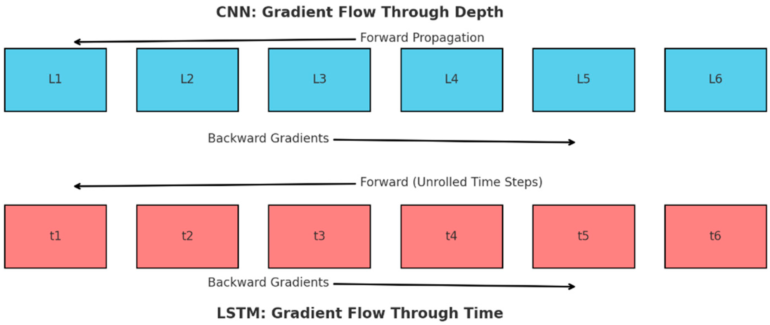
2.2. Vanishing and Exploding Gradient Problems

Vanishing and exploding gradients are critical challenges in training deep neural networks, particularly recurrent neural networks (RNNs). These issues can result in suboptimal performance or complete training failure [13]. Vanishing gradients occur when gradients shrink excessively, impairing the network’s ability to learn long-term dependencies. Conversely, exploding gradients happen when gradients grow uncontrollably, leading to instability and divergence during training.

Galimberti et al. [27] proposed Hamiltonian Deep Neural Networks (H-DNNs) to maintain non-vanishing gradients irrespective of network depth. Additionally, Ma et al. [28] introduced the HSIC bottleneck, replacing traditional cross-entropy loss and backpropagation to alleviate both vanishing and exploding gradients.

Vanishing Gradients: When the derivatives of the activation functions are less than one, the process of repeated multiplication during backpropagation results in an exponential diminishment of gradients:

$${\displaystyle \frac{\partial L}{\partial W}}\approx \prod _{l=1}^L{f}^{\prime \left(z^{\left[l\right]}\right)}· W^{\left[l\right]}$$

(4)

As $L\to \mathrm{\infty }$, gradients tend to approach zero, particularly when using sigmoid or tanh activation functions. In deep neural networks that employ these activation functions, the gradients in the initial layers can become negligible, effectively impeding the learning process.

Exploding Gradients: On the one hand, when the magnitudes of weights or derivatives of activations are greater than one, or if the network is not properly scaled, gradients can become unbounded as they move backward. In severe situations, the norm of the gradients can grow exponentially with network depth. This results in unstable updates and the risk of numerical overflow, which causes the training process to diverge.

$${\displaystyle \frac{\partial L}{\partial W}}~\prod _{l=1}^{L}c, where c>1 \Rightarrow Explosion$$

(5)

These challenges can impede convergence, slow down learning, or even completely halt a network’s training process. The development of the Xavier and He Initialization methods was specifically motivated by the need to address vanishing and exploding gradients through appropriate variance scaling. By starting with well-scaled weights, the network is more likely to maintain appropriate signal magnitudes throughout, particularly when used in conjunction with suitable activation functions and normalization techniques. Activation functions play a vital role in nonlinear transformation and directly affect gradient propagation (Figure 1).

Establishing proper initial weights is essential for stabilizing activations and gradients during both forward and backward propagation. Forward propagation computes outputs by passing input data through each network layer, while backward propagation calculates gradients to update weights based on errors [29]. Traditional backpropagation, although effective, faces limitations in biological plausibility and neuromorphic efficiency due to its reliance on separate forward and backward passes, exact error transmission, and nonlocal weight updates [30]. Solutions such as the Information Retention Network (IR-Net) mitigate these issues by using Libra Parameter Binarization to balance weights during forward propagation and an Error Decay Estimator to approximate gradients efficiently during backward propagation [29]. Additionally, mean squared quantization error (MSQE) regularization reduces discrepancies between forward and backward passes, particularly in low-precision networks [31]. The role of initialization becomes even more critical when comparing deep feedforward architectures, like CNNs, with recurrent models such as RNNs and LSTMs. In CNNs, depth refers to the number of sequential layers, requiring gradients to propagate backward across each layer. In contrast, RNNs and LSTMs represent depth through time, with gradients flowing backward over many time steps. In both architectures, poor initialization leads to signal degradation, either across layers in CNNs or across time steps in LSTMs, resulting in vanishing gradients and impaired learning (Figure 2).

2.3. Related Works

Recent advancements in weight initialization extend beyond the foundational methods to specialized strategies that address challenges such as vanishing and exploding gradients. Orthogonal initialization has proven effective in maintaining gradient stability, particularly in deep convolutional networks and recurrent neural networks [32,33]. It ensures the preservation of variance across layers, which is critical for training stability [6,34]. Chaos-based initialization methods, such as those utilizing Lorenz attractors, introduce structured randomness. These methods improve coverage of the parameter space and enhance convergence speed over traditional Gaussian-based initializations [9]. Mutual Information-based Initialization (MIWI) focuses on maximizing the mutual information between neuron activations and target outputs, particularly beneficial for networks with sigmoid activations. This method helps mitigate gradient saturation and maintains neuron sensitivity [35]. Metaheuristic optimization techniques, including Genetic Algorithms (GAs) and Particle Swarm Optimization (PSO), treat initialization as a global search problem. These approaches discover robust weight configurations that reduce the risk of poor local minima [7,11]. Polynomial-based initialization, such as the Linear Product Structure (LPS), models network computation as a polynomial expansion. This approach uses algebraic geometry to determine weight configurations that improve conditioning at the start of training [13]. Biologically inspired methods simulate synaptic weight distributions found in mammalian brains. Techniques like lognormal, modified lognormal, and skewed initializations produce long-tailed weight distributions that improve accuracy and generalization compared to conventional Gaussian distributions [36].

Table 1. Summary of advanced weight initialization techniques.

Initialization Method	Objective	Target Architecture	Key Advantage	References
Orthogonal	Variance preservation	Deep CNNs, RNNs, LSTMs	Stabilizes deep and recurrent models	[6,34]
Chaos-Based (Lorenz)	Structured randomness	Complex nonlinear models	Enhances diversity, accelerates convergence	[9]
Mutual Information (MIWI)	Information maximization	Sigmoid-based MLPs	Reduces saturation, improves signal sensitivity	[35]
Genetic/PSO Optimization	Global search optimization	General	Avoids poor local minima, robust initial states	[7,11]
Linear Product Structure (LPS)	Polynomial-based weight calculation	Polynomial-structured nets	Algebraically optimized initialization	[13]
Brain-Inspired (Lognormal, Skewed)	Biologically realistic weight distribution	Deep CNNs, general	Mimics synaptic diversity; boosts accuracy and convergence	[36]

summarizes these advanced initialization strategies, providing a comparison based on architectural suitability and key advantages.

Each of these techniques possesses distinct advantages and is optimally suited for specific network architectures or activation functions, as illustrated in Table 1. However, no single method comprehensively addresses all the training challenges in deep learning. Notably, there is a persistent gap in initialization strategies that can concurrently harness rigorous theoretical foundations.

3. Laor Initialization Method

This study assessed the impact of Laor Initialization in deep learning by integrating image classification and time-series forecasting tasks across diverse datasets and architectures. Laor Initialization uses k-means clustering to establish data-driven starting weights, aiming to reduce the initial loss and enhance convergence from the first epoch. Its main advantage is accelerating convergence and reducing early-stage errors compared to standard initializers. However, its reliance on clustering adds complexity, requiring adjustments based on dataset characteristics. The subsequent section details the experimental setup and Laor-based weight initialization process for CNN and LSTM models.

3.1. Data Collection

To assess Laor Initialization across deep learning models, this study used image data for classification and time-series data for regression. For time-series forecasting, daily gold prices (XAU/USD) from 1 January 2010 to 31 December 2020 were sourced from Yahoo Finance [37]. The dataset includes open, high, low, closing prices, and trading volume. The closing price was selected as the primary feature as it best reflects market sentiment. A sliding window approach converted time-series data into a supervised learning format, with inputs of 30-day closing price sequences and outputs of the subsequent day’s prices. After min–max scaling normalization, the dataset was split into 2400 records for training and 50 for testing and validation, ensuring the proper evaluation of new data. From the total 2450 daily records, 2400 entries covering nearly a decade trained the LSTM forecasting model, while 50 entries were used for testing and validation.

Table 2. Sample data of gold spot (GS).

No	Date	Close (USD)
1	3 September 2019	1545.90
2	4 September 2019	1550.30
3	5 September 2019	1515.40
4	6 September 2019	1506.20
5	9 September 2019	1502.20
6	10 September 2019	1490.30
7	11 September 2019	1494.40
8	12 September 2019	1498.70
9	13 September 2019	1490.90
10	16 September 2019	1503.10

summarizes the sample data structure and format used.

Two benchmark datasets were used: MNIST and CIFAR-10 [38]. The MNIST dataset contains 70,000 grayscale images of handwritten digits (60,000 for training and 10,000 for testing) at 28 × 28 pixels. CIFAR-10 comprises 60,000 color images (50,000 for training and 10,000 for testing) in 10 classes, each 32 × 32 pixels in RGB format. Both datasets were normalized to adjust the pixel values between 0 and 1.

3.2. Setting Parameters for Experiment

In the process of constructing an experiment, this study aimed to categorize the number of hidden layers into three distinct groups: the Input, Hidden, and Output layer. The activation function employed integrates both the ReLU and sigmoid functions (

Table 3. Structure of autoencoder with three hidden layers.

No.	Number of Neurons	Stimulating Function	Type of Layer
1	6	ReLU	Input layer
2	8	ReLU	Hidden layer
3	4	ReLU	Hidden layer
4	2	ReLU	Hidden layer
5	1	sigmoid	Output layer

). The average Root Mean Square Error (RMSE) was used as the loss function, and the Adam optimizer was selected for optimization. The experiment primarily utilized the Hold-Out Validation and K-Fold Cross-Validation Method. These hyperparameters were altered to evaluate the various weight-initialization techniques as shown in

Table 4. Hyperparameters of the model.

Parameters	Values
Epoch	1–200
Batch size	8, 16, 32, 64, 128, 256, 512
Optimizer	Adam
Loss function	Root Mean Square Error (RMSE)
Learning rate	0.1, 0.01, 0.001, 0.0001
Validation Methods	Hold-Out Validation Method (80% train and 20% test) K-Fold Cross-Validation Method

.

3.3. Procedure of Laor Initialization Method

Backpropagation and feedforward networks are integral to neural network training. Each epoch involved backward and forward propagation. Weight initialization is crucial during each epoch, as it affects information’s transmission through the network layers, influencing learning speed, convergence rate, and performance [7]. A poor initialization can cause vanishing or exploding gradients, thereby impeding network learning. Laor Initialization introduces a new method for weight initialization. This study does not address the selection of an appropriate variance for weight initialization owing to the increased complexity with more layers. The proposed method constrains the weights to prevent gradient problems. Weights and biases were configured to assess the effectiveness of the constraints. The method uses data collection for the initial configurations and the average of clusters with the lowest forward computation error as the default weight. The steps for Laor Initialization are shown (Figure 3).

3.3.1. Weight Initialization Using K-Means Clustering

The Laor Initialization method improves the starting weights of a neural network by evaluating multiple sets of random weights and using k-means clustering to determine the optimal initial point. The process is as follows:

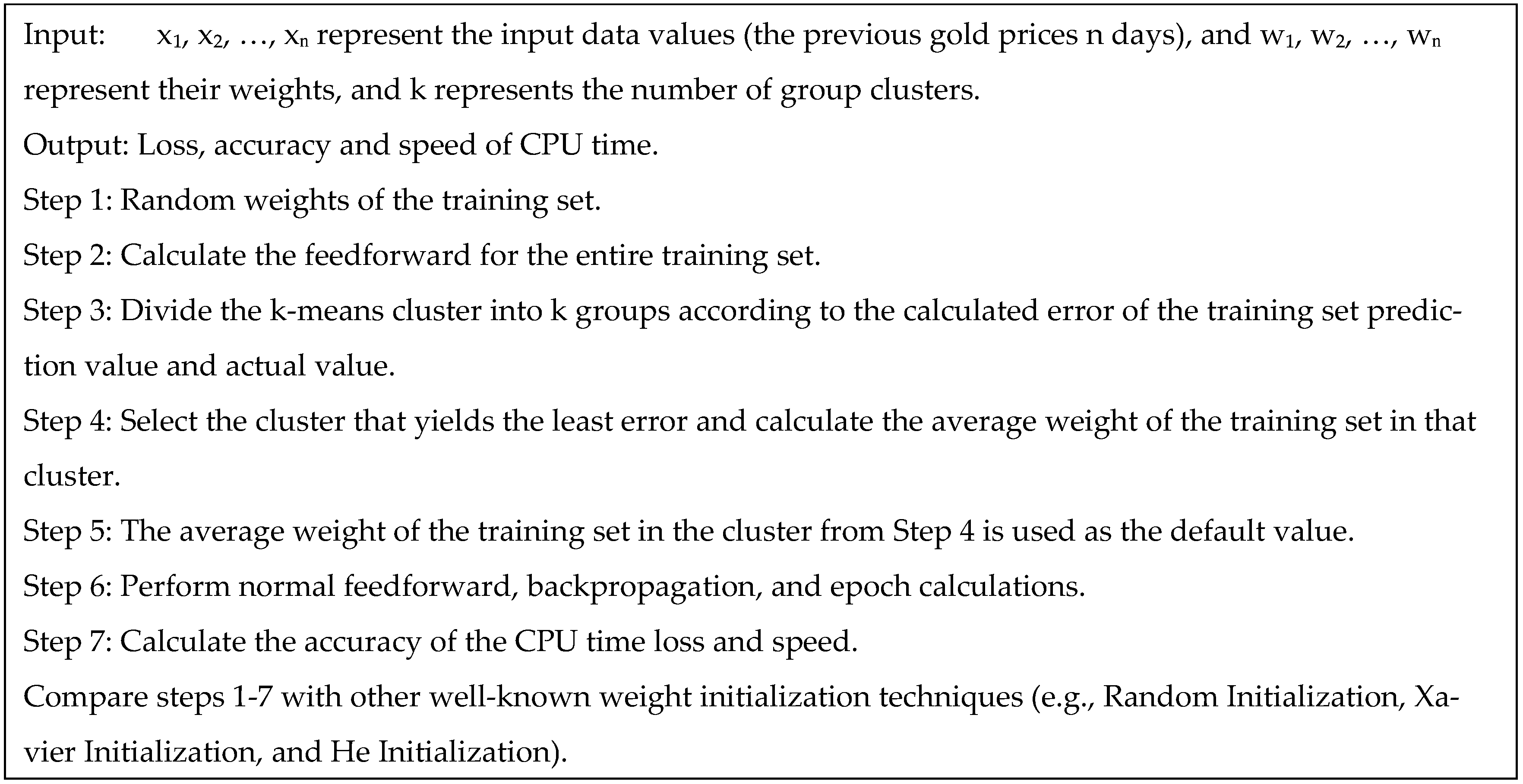
• Random Weight Initialization: Start by generating several random weight vectors (candidates for initialization). Each weight vector $W^{\left(0\right)}$ is sampled from a distribution, for example, $W^{\left(0\right)}~N\left(\mu ,{\sigma }^2\right)$, where μ is the mean, and σ2 is the variance of the normal distribution.
• Feedforward Computation: Each potential weight vector undergoes a forward pass on the training dataset to generate the predictions. If $x_{ji}$ denotes the $i$-th feature of the $j$-th training sample, then the predicted output for sample $j$ is calculated as the weighted sum of inputs using the candidate weights, $y_{{pred}_j=\sum _{i=1}^n{w}_i{x}_{ji}}$
• Compute RMSE Error: Evaluate the prediction error of each weight candidate using the Root Mean Square Error (RMSE) over all $m$ training samples. For a given weight vector, the RMSE is calculated as

  $${\mathit{E}}_{\mathit{j}}=\sqrt{{\displaystyle \frac{1}{\mathit{m}}}\sum _{\mathit{j}=1}^{\mathit{m}}{\left({\mathit{y}}_{{\mathit{a}\mathit{c}\mathit{t}\mathit{u}\mathit{a}\mathit{l}}_{\mathit{j}}-}{\mathit{y}}_{{\mathit{p}\mathit{r}\mathit{e}\mathit{d}}_{\mathit{j}}}\right)}^2}$$

  (6)

  where $y_{{actual}_j}$ is the true target value for sample $j$. A lower $E$ indicates that this weight initialization performs better on the first forward pass.
• K-Means Clustering: Once errors $E$ are computed for each candidate weight vector, apply k-means clustering to group these error values into $k$ clusters. Denote the set of error values in cluster $k$ as $C_k=\left\{E_j|j\in S_k\right\},$ where $S_k$ is the index set of weight candidates belonging to that cluster.
• Optimal Cluster Selection: Identify which cluster has the lowest average error. Formally, selecting meaning cluster $k^{\mathrm{*}}$ yields the smallest mean RMSE. This cluster represents the group of initial weight vectors that performed best in the first forward pass.

  $${\mathit{k}}^{\mathbf{*}}=\mathbf{arg}{\mathit{m}\mathit{i}\mathit{n}}_{\mathit{k}}{\displaystyle \frac{1}{\left|{\mathit{C}}_{\mathit{k}}\right|}}\sum _{\mathit{j}\in {\mathit{S}}_{{\mathit{k}}^{\mathbf{*}}}}{\mathit{E}}_{\mathit{j}}$$

  (7)
• Weight Initialization with Cluster Mean: Compute the new initial weights as the average of the weight vectors in the best cluster $k^{\mathrm{*}}$. Let $W_j$ be the weight vector for candidate $j$. The chosen initialization is that which is the mean of all weight vectors in the lowest-error cluster. This averaged weight vector serves as the initialized weight for the network, providing a data-informed starting point for training.

  $${\mathit{W}}_{\mathit{i}\mathit{n}\mathit{i}\mathit{t}}={\displaystyle \frac{1}{\left|{\mathit{S}}_{{\mathit{k}}^{\mathrm{*}}}\right|}}\sum _{\mathit{j}\in {\mathit{S}}_{{\mathit{k}}^{\mathrm{*}}}}{\mathit{W}}_{\mathit{j}}$$

  (8)

3.3.2. Feedforward Computation

With the weights initialized, the network performs a standard feedforward computation to produce outputs:

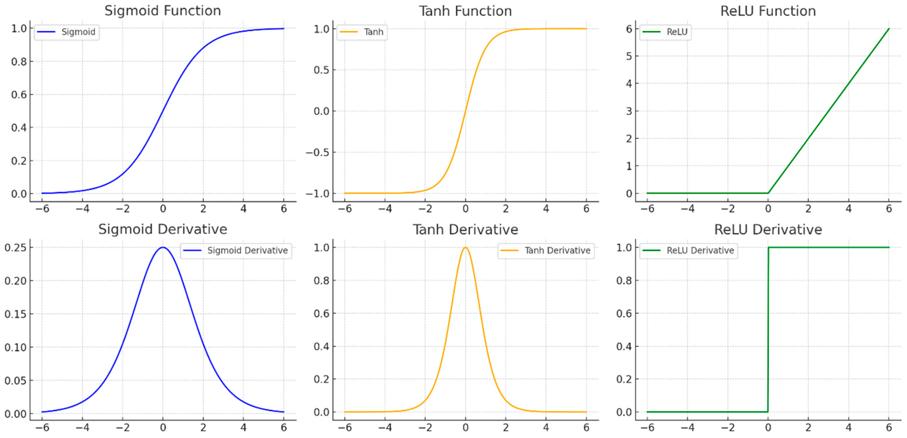
• Hidden Layer Activation (ReLU): As input data $X$ propagates through each hidden layer, apply the Rectified Linear Unit activation to the weighted sum plus bias. For a given hidden neuron with a weight vector $W$ and bias $b$, the activation is $A_{hidden}=\max \left(0,WX+b\right)$ The ReLU function outputs 0 for any negative input and passes positive values through unchanged, introducing nonlinearity and mitigating the vanishing gradient problem in deep networks.
• Output Layer Activation (sigmoid): For binary classification or output probabilities, sigmoid activation is used at the output layer. If $z=W{A}_{hidden}+b$ is the linear combination of the final hidden layer outputs, the sigmoid produces $A_{output}={\displaystyle \frac{1}{1+e^{-z}}}$, which squashes $z$ into the range [0, 1] [0, 1] [0, 1]. This output can be interpreted as a probability or a scaled prediction. (For regression tasks, a linear output might be used instead of a sigmoid).

3.3.3. Loss Function Calculation

After the forward pass, the network performance is measured using a loss function. In this case, the Root Mean Square Error (RMSE) is used to quantify the difference between the predictions and the actual targets:

$${\mathit{L}}_{\mathit{j}}=\sqrt{{\displaystyle \frac{1}{\mathit{m}}}\sum _{\mathit{j}=1}^{\mathit{m}}{\left({\mathit{y}}_{{\mathit{a}\mathit{c}\mathit{t}\mathit{u}\mathit{a}\mathit{l}}_{\mathit{j}}-}{\mathit{y}}_{{\mathit{p}\mathit{r}\mathit{e}\mathit{d}}_{\mathit{j}}}\right)}^2}$$

(9)

where $m$ is the number of samples. This is the same formula as in the initialization step, which is now viewed as the loss to be minimized during training. A smaller $L$ indicates that the model’s predictions $y_{pred}$ are closer to the true values $y_{actual}$ on average.

3.3.4. Backpropagation and Weight Updates

To train the network, the model iteratively updates its weights via backpropagation and an optimization algorithm:

• Weight Update Using Adam Optimizer: The gradient of the loss with respect to each weight ${\displaystyle \frac{\partial L}{\partial W}}$ is computed through backpropagation. The weights are then updated in the opposite direction to the gradient. For example, a simple gradient descent update at iteration $t$ would be

  $$W^{t+1}=W^t-\mathsf{\eta }{\displaystyle \frac{\partial L}{\partial W}},$$

  (10)

  where η is the learning rate. The Adam optimizer improves upon the basic gradient descent by adapting the learning rate for each weight using momentum and RMSprop techniques. It keeps moving averages of past gradients and squared gradients to formulate an adaptive update, but the core idea remains adjusting $W$ slightly in the direction that most reduces the loss.

3.3.5. Performance Metrics’ Evaluation

Several strategies are employed to evaluate the performance and ensure that the training process is effective.

• Convergence Check: Continuously monitor the loss $L$ during training. If $L$ falls below a predefined threshold $ϵ$(i.e., if $L$ < $ϵ$), or if $L$ stops changing significantly, the training can be stopped early. This check prevents overtraining and saves time once the model converges.
• Batch Size Analysis: The choice of mini-batch size $B$ (number of samples per gradient update) can affect training speed and stability. Common batch sizes to try are 8, 16, 32, 64, 128, 256, etc. The RMSE can be evaluated for different $B$s to see which yields the best trade-off. Smaller batches introduce more stochastic noise in the gradient, whereas larger batches provide more stable and accurate gradient estimates but may converge to sharp minima or take longer per epoch.
• Learning Rate Optimization: Test multiple learning rates $\mathsf{\eta }\in \left\{0.1, 0.01, 0.001, 0.0001\right\}$ to find an optimal value. The learning rate controls the step size during the weight updates. If η is too high, the training might diverge or oscillate; if it is too low, the convergence will be very slow. An optimal value of η minimizes the training time while maintaining stability.
• Cross-Validation (K-Fold): To ensure the model generalizes well, use $K$-fold cross-validation. Split the dataset into $K$ folds and perform the training $K$ times, each time holding out one fold as the validation set and using the remaining $K-1$ folds for training. Compute the validation loss for each fold $L_k$, then calculate the average validation loss

  $$L_{avg}={\displaystyle \frac{1}{k}}\sum _{k=1}^K{L}_k$$

  (11)
  A low and consistent $L_{avg}$ across folds indicates good generalization. This technique helps in selecting hyperparameters (like $B$ and η above) and in detecting overfitting.
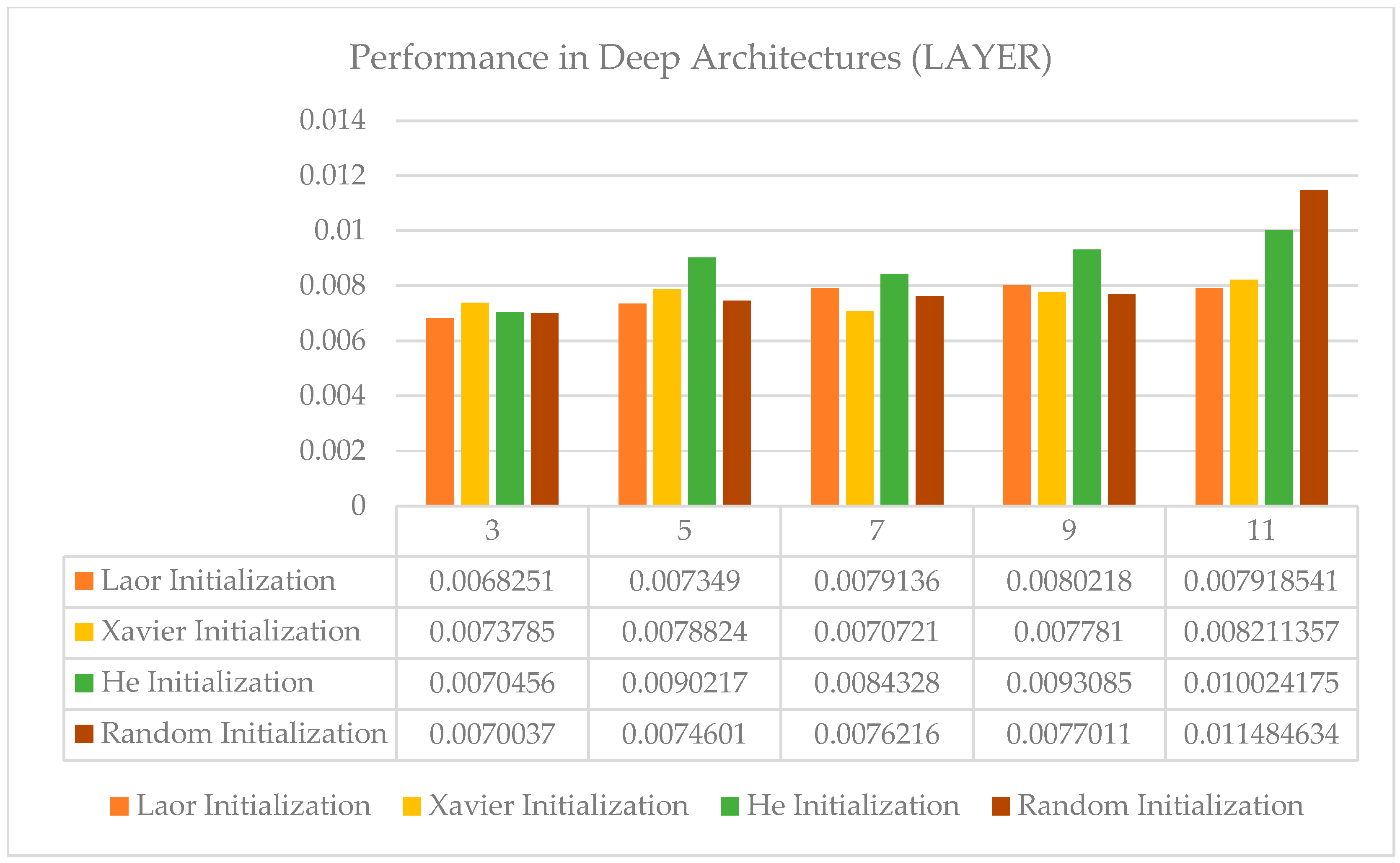
• Network Depth Effect: Experiments with different network depths (number of layers), such as 3, 5, 7, 9, and 11 layers, and a comparison of their resulting RMSEs. Increasing the depth can allow the model to learn more complex patterns, but it may also introduce challenges, such as vanishing gradients or overfitting. By tracking the performance, one can determine whether a deeper network actually improves the accuracy or whether a simpler architecture is sufficient.
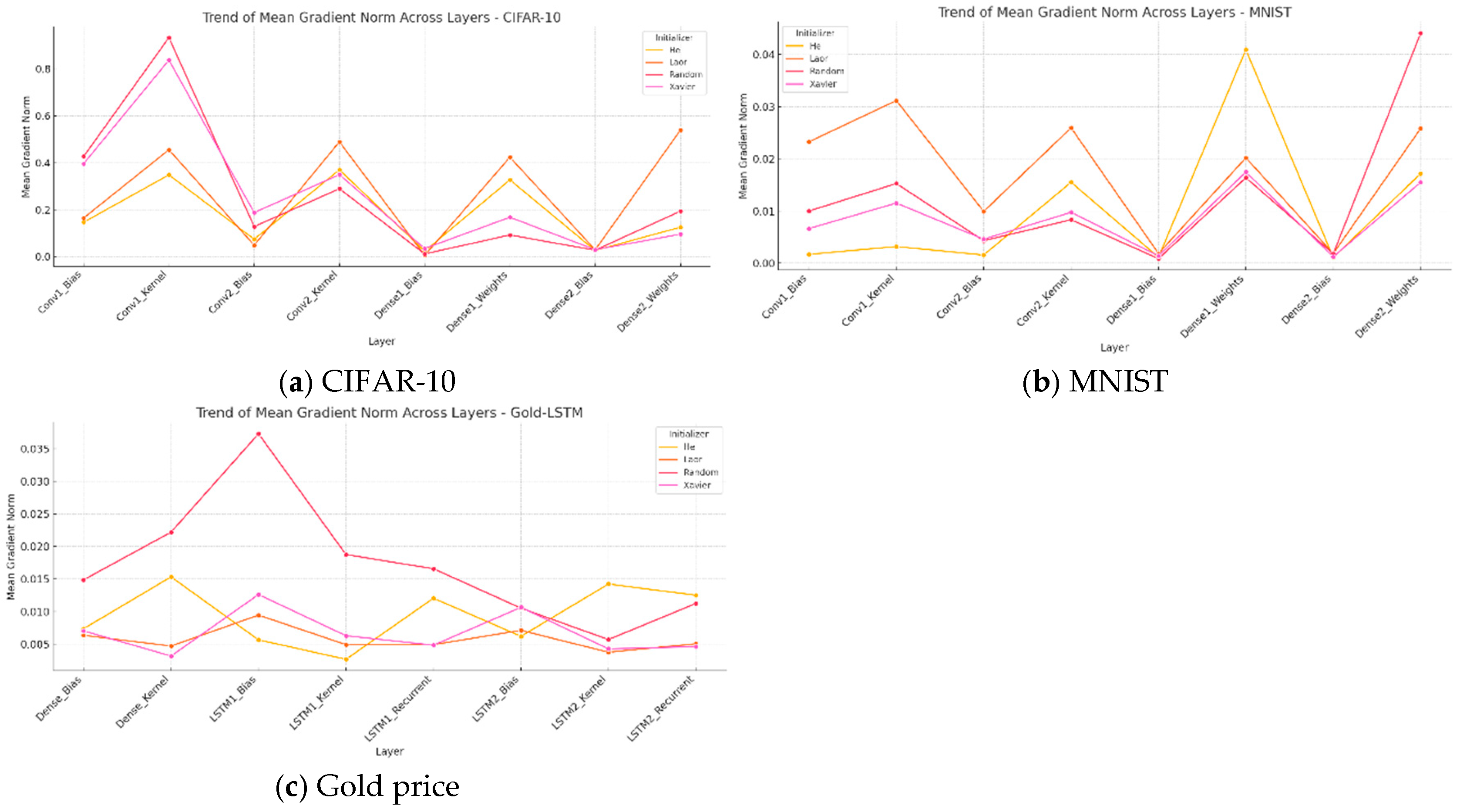
• Gradient Norm Analysis: A method for diagnosing the gradient scale during neural network training that provides insights into the error signal propagation through layers. By calculating the L2 norm of the loss function gradient relative to the model parameters, this approach assesses whether the gradients can effectively update the weights. Low-gradient norms indicate vanishing gradients, hindering learning by preventing significant weight updates in the deep models. Conversely, excessive gradient norms can lead to exploding gradients and unstable learning. Gradient Norm Analysis uses the average gradient norm per layer, standard deviation (SD), and coefficient of variation (CV) to evaluate magnitude and consistency. Categorizing norms into vanishing (norm < 0.01), stable (0.01 ≤ norm ≤ 1.0), and exploding (norm > 1.0) groups helps to identify susceptible layers and assess weight initialization effects.

4. Results and Discussion

This section evaluates Laor Initialization by comparing it with the Random, Xavier, and He Initialization methods. The assessment examined performance metrics, including the Root Mean Square Error (RMSE), convergence rate, and training time (CPU seconds) for classification and regression tasks. By implementing Laor Initialization in convolutional and recurrent neural networks, this study explores its ability to accelerate learning and enhance training stability. This analysis interprets the results and highlights the key findings of Laor’s performance across experimental contexts.

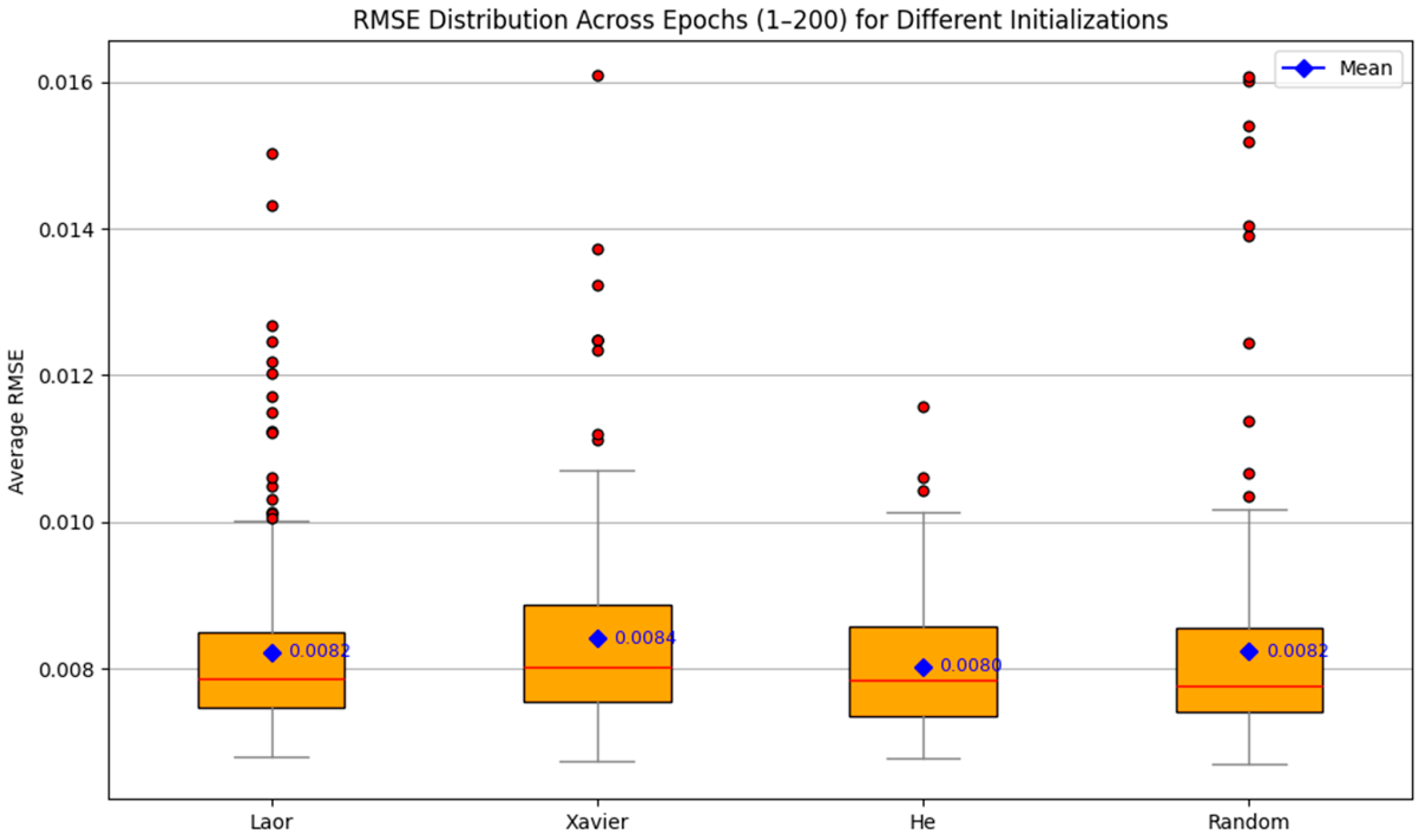
4.1. RMSE Trajectories over Epochs

The evaluation focuses on performance indicators, such as RMSE and training duration, for both classification and regression tasks to assess the practical effectiveness of each approach. Laor Initialization addresses this issue by initializing the model with weight clusters derived from an error-informed search and effectively selecting candidates that minimize the initial forward-pass loss. For this study, the following hyperparameters were established: learning rate of 0.001, Adam optimizer, batch size of 32, softmax activation function, and epoch range of 0–200. As illustrated in Figure 4, there was a comparison of RMSEs over 200 training epochs for networks initialized using the Laor, Random, Xavier, and He methods.

The enhanced box plot in Figure 4 provides a statistical comparison of the RMSE distributions across 200 training epochs for the four weight initialization strategies: Laor, Xavier, He, and Random. Laor Initialization shows a strong performance, with a mean RMSE of approximately 0.0082 and a median lower than those of Xavier and Random, indicating effective convergence throughout training. The narrow interquartile range (IQR) of Laor demonstrates its robustness and stability, showing fewer fluctuations compared with Xavier and Random Initialization, which display wider IQRs and more outliers. Although He Initialization shows slightly better central RMSE values, it presents a broader range and higher variability during mid-to-late epochs, where a minor performance degradation occurs. Xavier Initialization, although competitive early on, showed greater variability with its wider box and high-value outliers, suggesting less predictability in extended training. Random Initialization showed the highest inconsistency, with a high mean RMSE and wide error range, confirming its reliability issues. This visualization supports the Laor Initialization as a reliable strategy, particularly for long training epochs and consistent convergence. Its low dispersion, competitive mean RMSE, and stable trajectory make it well-suited for deep LSTM networks, where initialization is crucial for preventing gradient-related issues.

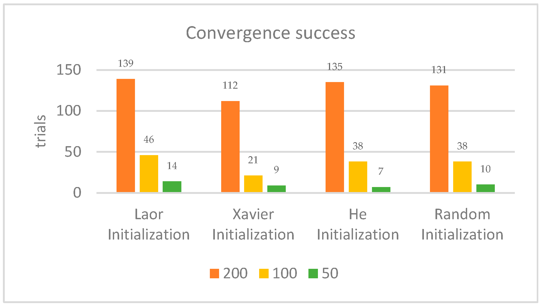
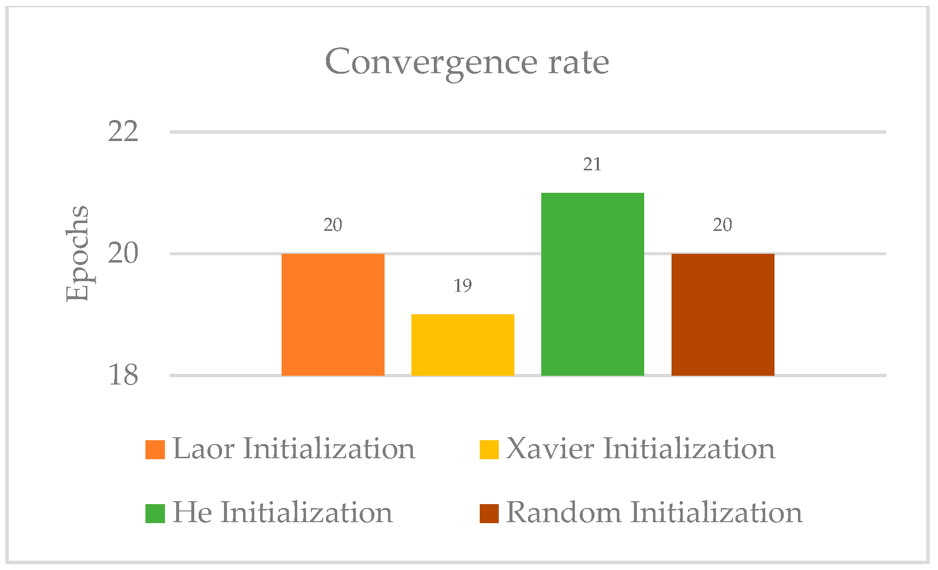
4.2. Convergence Success and Rate

The convergence of neural networks is influenced by both the initial conditions and the capacity of the optimizer to effectively utilize gradient data. The study evaluated convergence based on two criteria: (1) convergence success is the number of trials for which the algorithm reached the predefined convergence criteria, defined as achieving an RMSE of 0.00822697 (convergence criteria or averaging all of the error functions) or less, and (2) convergence rate is the number of epochs needed for the training to converge, which pertains to the number of epochs required to reach an RMSE of 0.00822697 or lower. (As shown in Figure 5 and Figure 6).

The findings in Figure 5 indicate significant variations among the methods. Laor Initialization demonstrated the highest success in convergence, achieving 139, 46, and 14 successful runs under 200, 100, and 50 trials, respectively, followed by He Initialization, with 135, 38, and 7, followed by Random Initialization, with 131, 38, and 10, and finally Xavier initialization, with 112, 21, and 9. These results match what previous studies have shown, as Laor Initialization methods help keep the variation in activation steady across layers, leading to stable gradients and better learning.

Figure 6 highlights the convergence rate defined by the number of epochs required for a model to achieve an RMSE of 0.00822697. The results demonstrate that He Initialization achieved the highest epoch frequency (21) where the RMSE was below the specified threshold (≤0.00822697), closely followed by Laor Initialization and Random Initialization, each with 20 epochs. The Xavier Initialization exhibited the lowest performance, with 19 epochs. These findings indicate that Laor Initialization exhibits a stable and competitive performance, comparable to He Initialization and is superior to Xavier Initialization in this context. The superior performance of He Initialization may be attributed to its compatibility with the ReLU activation functions. However, the differences among the methods were relatively minor, suggesting that further statistical analysis is necessary to ascertain whether these differences are statistically significant.

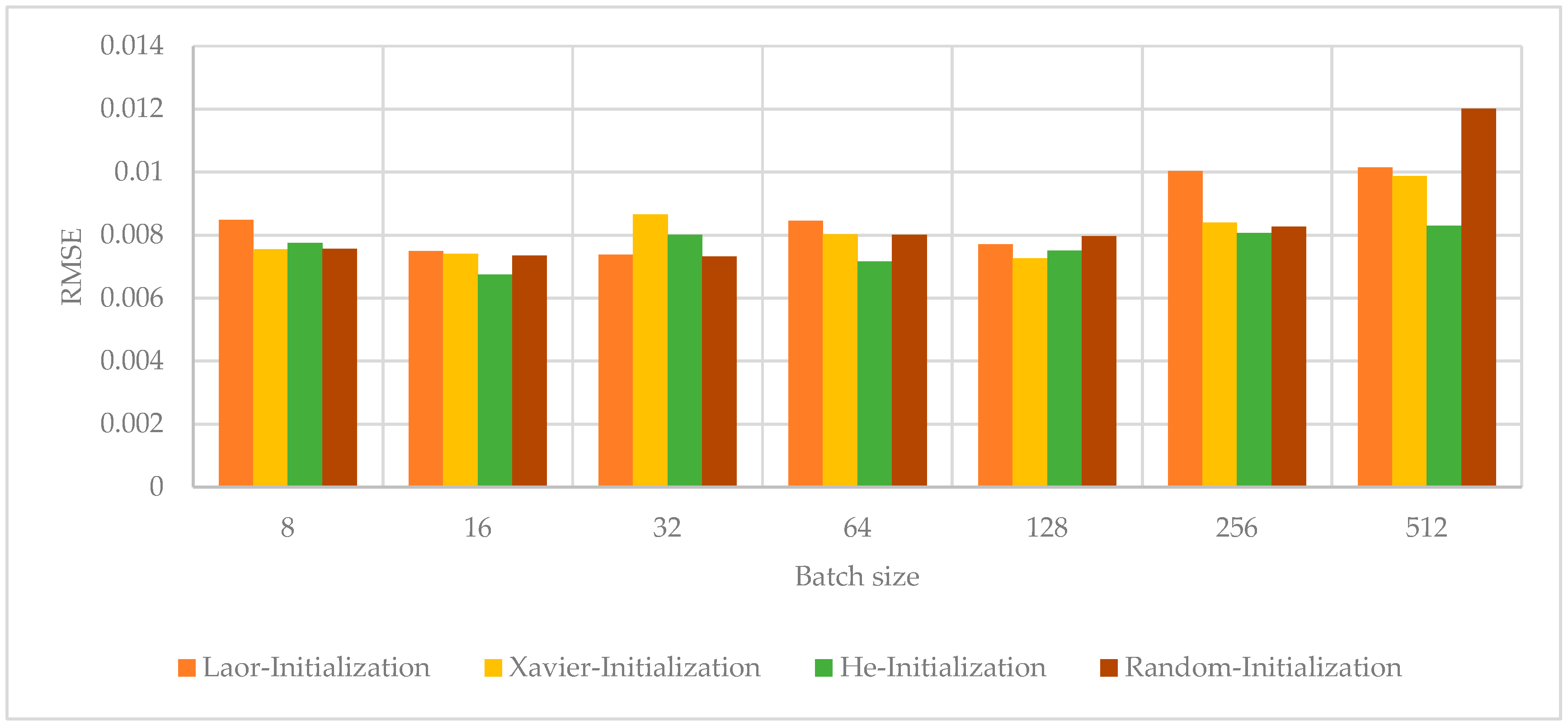
4.3. Interaction with Batch Size

Batch size [39], defined as the quantity of data utilized in the gradient estimation process, is a critical hyperparameter that requires adjustment prior to initiating the training process. Numerous studies have investigated the effects of batch size on network performance, specifically in terms of network accuracy and convergence time, to determine whether small or large batches are more effective. In our experiment, we used the following batch size values: 8, 16, 32, 56, 128, 256, and 512. Batch size refers to the amount of data required to train a single forward and backward pass. Figure 7 presents a comparison of the average RMSE across batch sizes for Laor Initialization and benchmarks.

Figure 7 illustrates the average RMSEs of the neural networks trained using various weight initialization methods (Laor, Xavier, He, and Random,) across a spectrum of batch sizes. This analysis provides valuable insights into the interaction between the batch size and initialization strategy. The batch sizes assessed were 8, 16, 32, 56, 128, 256, and 512. The findings indicate that Laor Initialization achieves optimal performance at a batch size of 32, recording the lowest average RMSE among all the evaluated methods. This suggests that Laor’s initialization strategy is particularly well-suited to the training dynamics present at moderate batch sizes, where gradient estimates effectively balance stochasticity and stability. At a batch size of 32, the model benefits from sufficient mini-batch diversity for generalization without the training noise associated with smaller batches or the reduced variability characteristic of very large batches. It is observed that the RMSE benefit of Laor diminishes slightly at both ends of the batch size spectrum. With smaller batch sizes, such as 8 and 16, the increased gradient noise can disrupt the optimized starting point provided by Laor, resulting in a more unpredictable training process and partially negating the advantage of a well-informed initialization. Conversely, with larger batch sizes, such as 256 and 512, while gradient updates become more stable, the lack of sufficient randomness may hinder the ability of the optimizer to escape shallow local minima, thereby reducing the impact of Laor’s advantageous initialization. The compatibility of Laor with medium-sized batches makes it particularly suitable for a wide range of real-world applications that aim to optimize both learning efficiency and generalization [40].

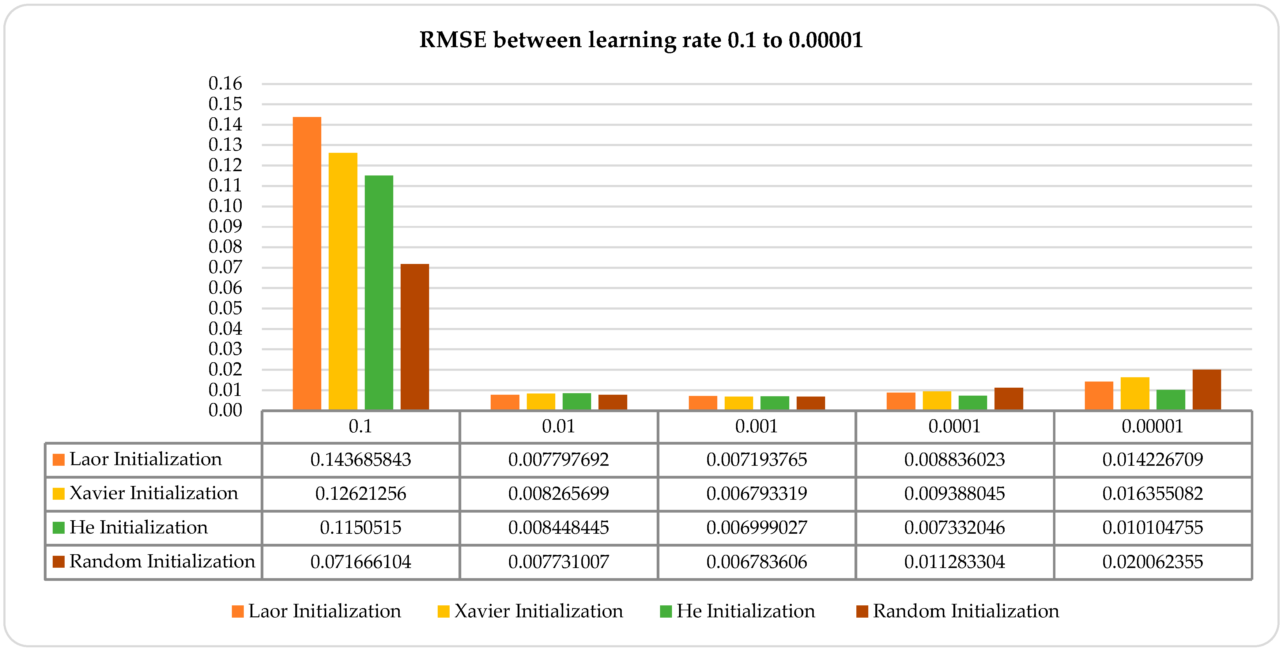
4.4. Sensitivity to Learning Rate

Figure 8 presents an analysis of various initialization strategies—Laor, Xavier, He, and Random—within the LSTM networks across different learning rates. These findings underscore the advantages of Laor Initialization under diverse optimization conditions. At a learning rate of 0.1, Laor exhibited the highest RMSE (0.1437), exceeding other methods, with Random Initialization (0.0717) demonstrating superior performance. This outcome suggests Laor’s sensitivity to aggressive parameter updates, which is attributed to its cluster-based weight configuration that amplifies gradients at larger step sizes. At a learning rate of 0.01, Laor’s performance markedly improved, achieving the lowest RMSE (0.00780) among all the methods. This indicates that Laor excels in stable environments where moderate updates facilitate a favorable convergence. At a learning rate of 0.001, the performance gap between the methods narrowed, with Xavier (0.00679) and Random (0.00678) slightly outperforming Laor (0.00719). In this context, performance is primarily influenced by the optimization dynamics rather than the initialization strategy. With a learning rate of 0.0001, Laor demonstrated resilience, achieving an RMSE (0.00884) lower than that of Xavier and Random, although higher than that of He Initialization (0.00733). This suggests that Laor maintains an adequate gradient flow even in slower-update regimes. At a learning rate of 0.00001, Laor performs robustly (0.01423), surpassing Xavier (0.01636) and Random (0.02006), while achieving the best RMSE (0.01010). Laor’s reasonable accuracy in low-gradient scenarios indicates that its initialization structure provides stability, even with minimal updates.

Overall, these results affirm that Laor Initialization is most effective when paired with a suitably tuned learning rate, particularly at approximately 0.01–0.001. This synergy promotes faster and more stable convergence and supports the broader recommendation of using the largest learning rate that does not destabilize training [41]. Practitioners are therefore encouraged to tune the learning rate alongside initialization to maximize training efficiency and performance.

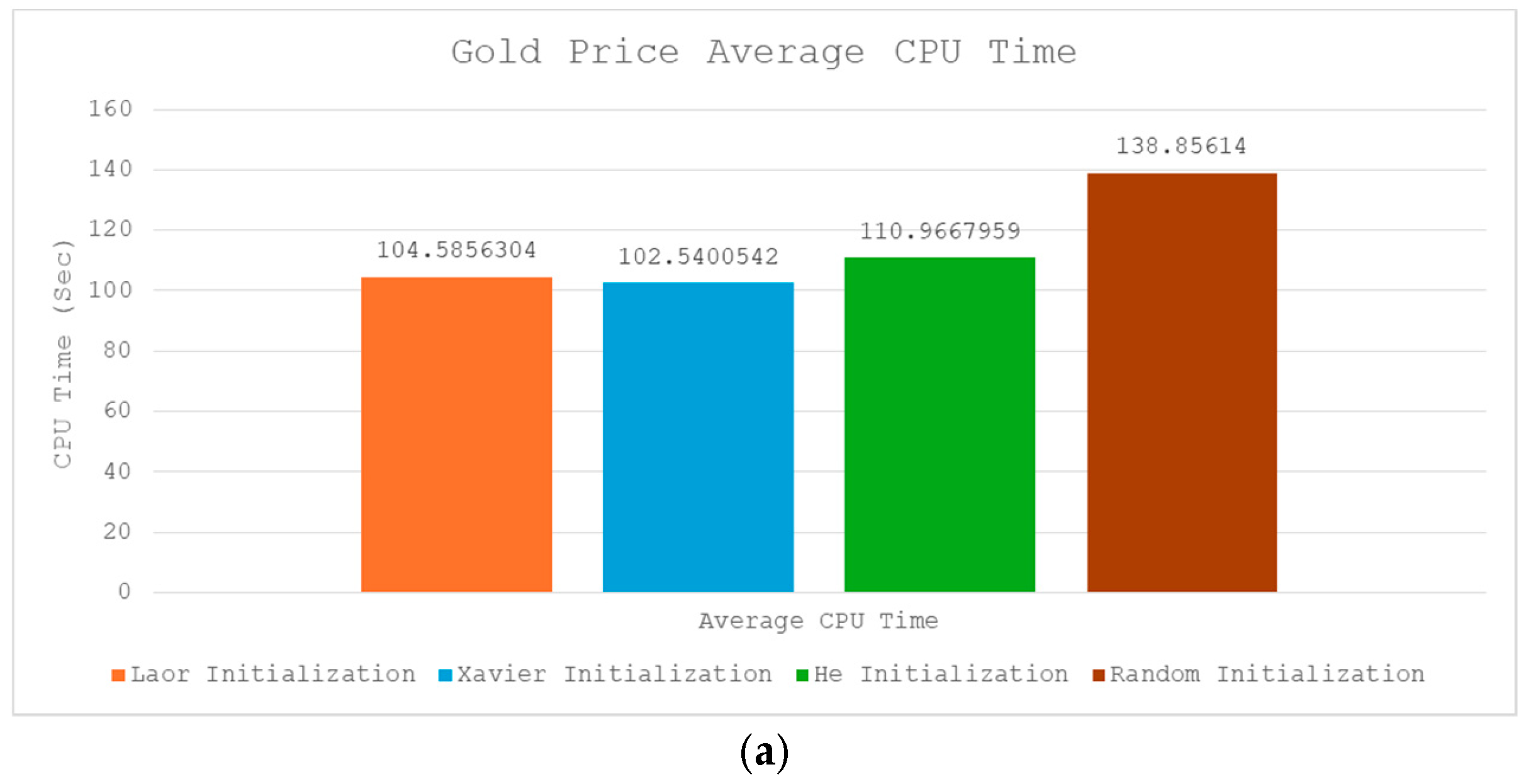
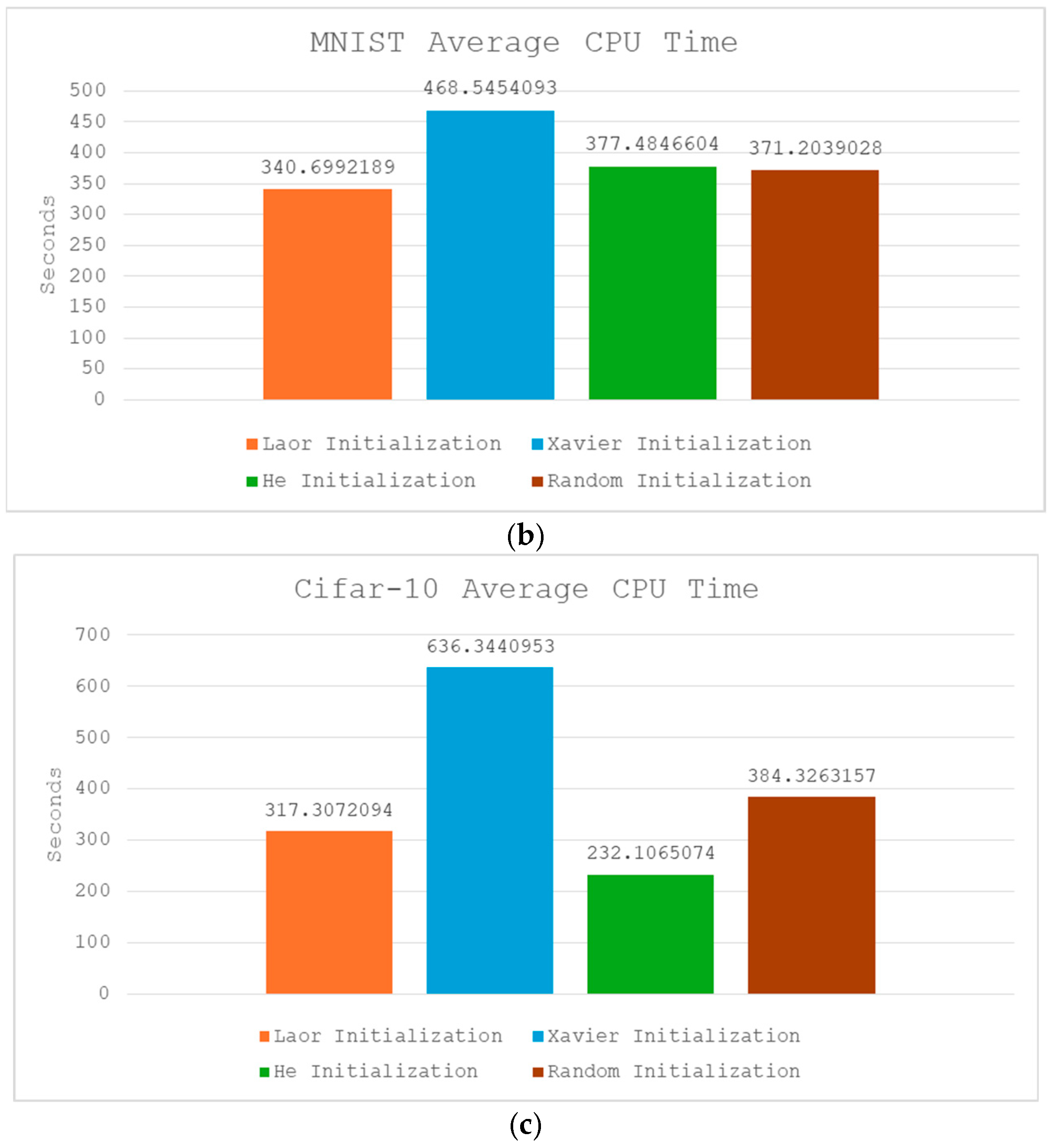
4.5. Computational Overhead and Efficiency (CPU Time)

Initialization methods often require a balance between computational efficiency and training effectiveness. Although Laor Initialization involves an initial clustering step based on the assessment of forward-pass errors, it unexpectedly contributes positively to the overall training duration. In this study, an experiment was conducted with the following parameters: a learning rate of 0.001, batch size of 32, and 100 epochs. The results are shown in Figure 9.

Figure 9 presents a comprehensive analysis of the CPU training times for various weight initialization methods (Laor, Xavier, He, and Random) across three benchmark datasets: Gold price (utilizing LSTM for regression), MNIST (employing CNN for digit classification), and CIFAR-10 (utilizing CNN for object classification). For the Gold price dataset (Figure 9a), Laor Initialization achieved a training time of 104.58 s, significantly outperforming Random Initialization (138.86 s) and He Initialization (110.97 s) while remaining closely competitive with Xavier Initialization (102.54 s). In the MNIST digit classification task, Laor continued to demonstrate superior performance, completing training in 340.69 s, surpassing Random (371.20 s) and He (377.48 s). Notably, Laor outperformed Xavier Initialization, which required 468.54 s. The CIFAR-10 dataset (Figure 9c), which is recognized for its complexity and high-dimensional RGB input space, poses significant computational challenges. Notably, the He Initialization achieved the fastest training time (232.10 s), followed by the Laor Initialization at 317.30 s. Although Laor was not the fastest, it notably outperformed Random Initialization (384.32 s) and Xavier Initialization, which required a substantial 636.34 s. The underperformance of Xavier is likely due to its optimization of sigmoid/tanh activations, which are less prevalent in modern CNNs utilizing ReLU on CIFAR-10.

4.6. Generalization via K-Fold Cross-Validation

The K-Fold Cross-Validation Method involved dividing the dataset into training and testing subsets multiple times (k iterations). The primary objective of this technique is to evaluate the error rates of a model in a broadly applicable manner. In this study, the experiment was conducted with the following parameters: a learning rate of 0.001, a batch size of 32, and 100 epochs. As illustrated in Figure 10, the Laor Initialization resulted in a lower RMSE than the Xavier, He, and Random initializations.

Figure 10 illustrates RMSE outcomes obtained from a K-fold cross-validation analysis utilizing four distinct initialization techniques: Laor, Xavier, He, and Random. This figure presents the average RMSEs across all validation folds, offering a comprehensive assessment of the generalization capability of each method. Laor Initialization was characterized by the lowest RMSE of 0.00687, surpassing the other methods in terms of predictive accuracy. This consistent advantage, even with repeated dataset partitioning, highlights Laor’s robust generalization across various training–validation splits. In contrast, the Xavier and Random Initializations produced RMSEs of 0.00712 and 0.00715, respectively, both slightly higher than Laor, whereas He Initialization lagged further behind at 0.00768. Although these differences are numerically minor, they are significant in performance-critical tasks where even slight improvements in error rates can lead to substantial gains in real-world applications. The findings confirm that Laor’s error-informed clustering of initial weights not only accelerates the learning process but also enhances its cross-validation consistency. This robustness reduces the sensitivity of the model to data variability and enhances its reliability when applied to unseen samples.

4.7. Depth Scalability: Performance in Deep Architectures (LAYER)

Laor Initialization was developed with deep architectures in mind to address the prevalent issue of gradient degradation in such networks. Figure 11 shows the evaluation of its effectiveness across various network depths, specifically three, five, seven, nine, and eleven layers.

The results from Figure 11 provide significant insights into the scalability and robustness of Laor Initialization compared with established methods. At shallower depths, specifically in layers 3 and 5, Laor consistently surpassed all other strategies, achieving the lowest RMSE values of 0.00683 and 0.00735, respectively. This suggests that Laor’s initialization offers a highly effective starting point for learning in compact architectures. Its capacity to align the initial weights with the underlying input structure likely contributes to improved convergence behavior and reduced learning errors in the early stages of training. As the network depth increases to seven and nine layers, Laor’s performance experiences a slight decline, with RMSE values increasing to 0.00791 and 0.00802. While these values remain competitive, outperforming He Initialization and remaining close to Random, Xavier Initialization demonstrates a slight advantage at these depths. This shift indicates that although Laor is not explicitly designed to preserve the signal variance across layers, it maintains reasonable stability even as the network becomes deeper. The decline in performance may be attributed to the compounded nonlinearities and gradient attenuation common in deeper LSTM networks; initialization strategies such as Xavier and He are specifically engineered to address these issues through variance scaling. Notably, at layer 11, the deepest tested architecture, Laor Initialization once again delivered the best performance with an RMSE of 0.00792, surpassing Xavier (0.00821), He (0.01002), and Random (0.01148). This unexpected resurgence underscores Laor’s potential for resilience in deep network settings, where it evidently maintains the weight distribution in a manner that supports a stable gradient flow.

4.8. Gradient Norm Stability Analysis

The consistency and magnitude of gradient norms were meticulously analyzed using various initializers (Laor, Xavier, He, and Random) and datasets (MNIST, CIFAR-10, and Gold price) to assess training robustness and the potential for gradients to either vanish or explode. For each layer, the mean gradient norms, standard deviations (SDs), and coefficients of variation (CVs) were calculated over multiple interaction runs. The criteria for stability adhered to standard deep learning practices [4]: a mean gradient norm below 0.01 was classified as vanishing, a mean gradient norm above 1.0 was classified as exploding, and values ranging from 0.01 to 1.0 were considered stable.

Table 5. The mean, standard deviation, coefficient of variation (CV), and stability state were created, with risk points of vanishing gradients highlighted for further discussion.

Dataset	Initializer	Mean Gradient Norm	Std Gradient Norm	CV (Mean)	Vanishing Layers	Exploding Layers	Stable Layers
CIFAR-10	He	0.1802	0.1462	0.4456	0	0	8
	Laor	0.2695	0.2290	0.3448	1	0	7
	Random	0.2629	0.3043	0.3633	0	0	8
	Xavier	0.2624	0.2685	0.3034	0	0	8
Gold price	He	0.0095	0.0046	0.4366	4	0	4
	Laor	0.0058	0.0018	0.5997	8	0	0
	Random	0.0171	0.0096	0.4451	1	0	7
	Xavier	0.0067	0.0033	0.3841	6	0	2
MNIST	He	0.0103	0.0141	0.4365	5	0	3
	Laor	0.0175	0.0114	0.2230	3	0	5
	Random	0.0126	0.0139	0.3926	5	0	3
	Xavier	0.0085	0.0061	0.3755	5	0	3

summarizes the results, including stability classification and highlights of layers at risk for vanishing gradients.

Table 5 presents a comprehensive comparison of the gradient behavior across various datasets and initializers, assessed using four primary metrics: mean gradient norm, standard deviation, coefficient of variation (CV), and the counts of vanishing, exploding, and stable layers. Laor Initialization consistently exhibited competitive or superior mean gradient norms compared with standard initializers across all datasets. In the CIFAR-10 dataset, Laor achieved the highest mean gradient norm (0.2695), which supported the robust and consistent learning signals essential for maintaining deep feature extraction capabilities. In the MNIST dataset, Laor’s mean gradient norm (0.0175) surpassed that of Random and Xavier, indicating an enhanced early training stability in a relatively shallow CNN architecture. For the Gold price dataset, the mean gradient norms were generally lower across all initializers because of the recurrent nature of the architecture, but Laor’s slightly lower mean (0.0058) suggested a conservative approach that helped prevent instability without significantly increasing the risk of vanishing. The higher mean gradients associated with Laor in convolutional models are advantageous for ensuring an adequate signal propagation across layers during training, without causing numerical instability. Regarding the coefficient of variation, Laor achieved the lowest CV values in MNIST (0.2230) and relatively low values in CIFAR-10 (0.3448), indicating a more stable and consistent gradient behavior than He, Random, and Xavier. Although the CV for Laor in the Gold price dataset was somewhat higher (0.5997), this aligns with the known difficulty of maintaining stable gradients in recurrent networks; even so, Random and He also exhibited comparably high CVs, with Random reaching 0.4451. The lower CV values for Laor across the datasets underscore its ability to produce less variable and more reliable gradient magnitudes, contributing to a more predictable and stable model convergence.

In addition, Figure 12 illustrates the trend of mean gradient norms across network layers for each initializer and dataset, providing a visual depiction of how gradient magnitudes propagate throughout the network. This highlights the layer-wise consistency of Laor across varying architectures and tasks.

Figure 12 provides valuable insights into the performances of various initializers across different neural architectures. For the CIFAR-10 dataset, which involves a deeper and more complex CNN structure, Laor maintains the highest gradient magnitudes in the initial layers, with a smooth and gradual decrease as it progresses toward deeper dense layers. This suggests that Laor facilitates a more stable and efficient backpropagation path throughout the network depth. In contrast, He Initialization exhibits a more pronounced decline, particularly in Conv2_Bias and Dense2_Bias, whereas Xavier and Random show less consistent patterns, with some sudden fluctuations. Laor’s trend line is the most linear and progressive, highlighting its advantage in managing gradient decay over depth in complex visual feature hierarchies. For the MNIST dataset, Laor Initialization demonstrates a relatively flat and consistent gradient trajectory across all layers, maintaining significant gradient magnitudes in both the convolutional (Conv1_Kernel, Conv2_Kernel) and dense layers (Dense1_Weights, Dense2_Weights). Notably, only a slight decline was observed in the bias units, particularly in Dense1_Bias and Dense2_Bias. In contrast, the He and Xavier Initializations display a steeper downward trend, especially after the early convolutional layers, with several bias-related layers falling below the vanishing threshold (mean < 0.01). Random Initialization is characterized by greater fluctuations and irregularities in gradient norms, indicating inconsistencies in early training signal propagation. The Gold price dataset revealed a distinct pattern owing to its recurrent architecture. All the initializers generally show lower gradient norms, reflecting the known challenge of vanishing gradients in deep recurrent models. Laor demonstrates slightly improved stability in kernel-related weights (LSTM1_Kernel and LSTM2_Kernel), but the trend sharply declines in recurrent and bias terms (e.g., LSTM1_Recurrent and LSTM2_Bias), confirming that while Laor mitigates gradient collapse more effectively than He or Xavier, it still struggles with long-term gradient retention. Random exhibits irregular transitions between layers, and both He and Xavier display a more pronounced vanishing, particularly in the bias parameters. In summary, the trend graphs confirm that Laor Initialization maintains a more favorable and controlled gradient flow across both shallow and deep CNNs, with smoother transitions between layers and fewer critical drops. While improvements are evident even in LSTM models, further refinements are necessary to achieve a similar robustness in recurrent neural networks.

4.9. Summary of Findings and Proposed Improvements

The comprehensive experimental results indicate that Laor Initialization is a robust and effective alternative to traditional initialization methods such as Xavier, He, and Random Initialization. Across all the evaluated criteria, including convergence success rate (RMSE), convergence rate (epochs), stability at various depths, and gradient behavior, Laor consistently demonstrates advantages, particularly in moderately deep to deep network configurations. Laor achieved a lower RMSE than the Xavier and Random Initializations while maintaining a competitive convergence rate, reaching convergence within 20 epochs—faster than He (21 epochs) and comparable to Random but only slightly slower than Xavier (19 epochs). However, unlike Xavier, which compromises the convergence accuracy for speed, Laor achieves a balanced optimization between RMSE reduction and convergence rate. Notably, Laor exhibited the highest depth scalability among all the tested methods. In deeper architectures (e.g., 11 layers), Laor achieved the lowest RMSE, outperforming Xavier, He, and Random. This advantage is attributed to Laor’s cluster-based initialization strategy, which aligns weight distributions with input data clusters, enhancing forward-pass error stability and gradient propagation, as supported by recent research on data-driven initialization methods [42,43]. Despite its strengths, this study has two primary limitations. First, Laor demonstrated sensitivity to high learning rates (>0.01), which is a phenomenon consistent with other cluster-based or adaptive initialization techniques [44]. Second, the k-means clustering step introduces a modest computational overhead during initialization, which becomes more noticeable in high-dimensional models. Additionally, minor RMSE fluctuations occurred in mid-depth architectures (7–9 layers), although this does not negate Laor’s overall superiority at greater depths. In summary, the findings confirm that Laor Initialization delivers a strong balance between convergence accuracy, speed, and stability, outperforming or matching benchmark methods in most scenarios.

Table 6. Comparative summary of Laor Initialization against baseline methods.

Criteria	Laor	Xavier	He	Random
Convergence Success Rate	Low (0.00822)	Highest (0.00842)	Lowest (0.00803)	Moderate (0.00824)
Convergence Rate	Moderate (20)	Fastest (19)	Slowest (21)	Moderate (20)
RMSE Stability (IQR)	Narrow	Wide	Moderate	Widest
Gradient Stability	Best	Poor at deep networks	Moderate	Frequent vanishing/exploding
Depth Scalability (11 Layers)	Best (0.00792)	Unstable (0.00821)	Unstable (0.01002)	Unstable (0.01148)
Batch Size Sensitivity	Stable	Sensitive	Stable	Unstable
Learning Rate Sensitivity	Sensitive	Handles high LR	stable	unstable
CPU Time	Fastest on MNIST Moderate on CIFAR-10 and Gold Price	Fastest on Gold price Slowest on CIFAR-10 and MNIST	Fastest on CIFAR-10 Moderate on MNIST and Gold Price	Slowest on Gold price Moderate on CIFAR-10 and MNIST
Cross-Validation Robustness	Lowest RMSE	High RMSE	Moderate	High RMSE

summarizes the key findings, strengths, limitations, and comparative evaluations across all the initialization strategies.

5. Conclusions

This study introduced Laor Initialization, which is a data-driven weight initialization method for deep neural networks. This method integrates forward-pass error feedback with k-means clustering to determine optimal starting weights. In contrast to traditional methods, such as Random, Xavier, and He, Laor enhances training efficiency, convergence stability, and generalization performance. The experimental validation used three datasets: Gold price, MNIST, and CIFAR-10 across convolutional (CNN) and recurrent (LSTM) architectures. The results show that Laor achieved the lowest K-fold cross-validation RMSE of 0.00686, outperforming Xavier, He, and Random. For the convergence rate, Laor reached the target RMSE within 20 epochs, which was faster than He, equal to Random, and slightly slower than Xavier. The convergence success rate was 0.00822 for Laor, surpassing that of Xavier and Random and marginally higher than that of He. Laor exhibited the narrowest RMSE interquartile range (IQR), indicating a high training stability compared to He, Xavier, and Random. Gradient norm analysis confirmed Laor’s stability, with the lowest coefficient of variation (CV) on MNIST (0.2230), CIFAR-10 (0.3448), and Gold price (0.5997). No vanishing layers occurred in the CNN models, although eight vanishing layers persisted in the LSTM-based Gold price model. For computational efficiency, Laor achieved the fastest training time on MNIST and reduced the CPU time on Gold price by 24% compared to Random (104.58 s vs. 138.86 s). On CIFAR-10, Laor outperformed Xavier and Random but was slower than He. Laor performed optimally with a batch size of 32 and learning rates of 0.0001–0.01. Laor Initialization offers a robust alternative to conventional techniques, providing superior generalization, gradient stability, a narrower RMSE variability, and improved training efficiency. Future work should focus on enhancing Laor through dynamic variance scaling and adaptive clustering.

References

1. Kumar, S. On weight initialization in deep neural networks. arXiv 2017, arXiv:1704.08863. [Google Scholar] [CrossRef]
2. Lyu, Z.; Karns, J.; Desell, T.; Mkaouer, M.; Elsaid, A. An Experimental Study of Weight Initialization and Lamarckian Inheritance on Neuroevolution. In International Conference on the Applications of Evolutionary Computation (EvoApplications 2021); Springer: Cham, Switzerland, 2021; pp. 584–600. [Google Scholar] [CrossRef]
3. Zucchet, N.; Orvieto, A. Recurrent neural networks: Vanishing and exploding gradients are not the end of the story. arXiv 2024, arXiv:2405.21064. [Google Scholar] [CrossRef]
4. Glorot, X.; Bengio, Y. Understanding the difficulty of training deep feedforward neural networks. In Proceedings of the Thirteenth International Conference on Artificial Intelligence and Statistics (AISTATS 2010), Chia Laguna Resort, Sardinia, Italy, 13–15 May 2010; pp. 249–256. [Google Scholar]
5. He, K.; Zhang, X.; Ren, S.; Sun, J. Delving deep into rectifiers: Surpassing human-level performance on ImageNet classification. In Proceedings of the IEEE International Conference on Computer Vision (ICCV 2015), Santiago, Chile, 7–13 December 2015; pp. 1026–1034. [Google Scholar]
6. Saxe, A.M.; McClelland, J.L.; Ganguli, S. Exact solutions to the nonlinear dynamics of learning in deep linear neural networks. arXiv 2013, arXiv:1312.6120. [Google Scholar] [CrossRef]
7. Narkhede, M.V.; Bartakke, P.P.; Sutaone, M.S. A review on weight initialization strategies for neural networks. Artif. Intell. Rev. 2021, 55, 291–322. [Google Scholar] [CrossRef]
8. Darrell, T.; Donahue, J.; Krähenbühl, P.; Doersch, C. Data-dependent initializations of convolutional neural networks. arXiv 2015, arXiv:1511.06856. [Google Scholar] [CrossRef]
9. Jia, B.; Guo, Z.; Huang, T.; Guo, F.; Wu, H. A generalized Lorenz system-based initialization method for deep neural networks. Appl. Soft Comput. 2024, 167, 112316. [Google Scholar] [CrossRef]
10. Zhou, X.; Liu, S.; Qin, A.K.; Tan, K.C. Evolutionary neural architecture search for transferable networks. IEEE Trans. Emerg. Top. Comput. Intell. 2024, 9, 1556–1568. [Google Scholar] [CrossRef]
11. Xu, Z.; Chen, Y.; Vishniakov, K.; Liu, Z. Initializing models with larger ones. In Proceedings of the 12th International Conference on Learning Representations (ICLR 2024), Vienna, Austria, 7–11 May 2024. [Google Scholar]
12. Wang, Z.; Bhoyar, P.H.; Teoh, C.; Irfan, S.A. K-means Clustering. In Machine Learning Algorithms for Industrial Applications; Bentham Science: Sharjah, United Arab Emirates, 2023; pp. 194–211. [Google Scholar] [CrossRef]
13. Liu, M.; Du, X.; Shang, M.; Jin, L.; Chen, L. Activated Gradients for Deep Neural Networks. IEEE Trans. Neural Netw. Learn. Syst. 2023, 34, 2156–2168. [Google Scholar] [CrossRef]
14. Al-Abri, S.; Zhang, F.; Lin, T.X.; Tao, M. A Derivative-Free Optimization Method with Application to Functions with Exploding and Vanishing Gradients. IEEE Control Syst. Lett. 2020, 5, 587–592. [Google Scholar] [CrossRef]
15. Wong, K.; Dornberger, R.; Hanne, T. An Analysis of Weight Initialization Methods in Connection with Different Activation Functions for Feedforward Neural Networks. Evol. Intell. 2024, 17, 2081–2089. [Google Scholar] [CrossRef]
16. Li, H.; Perin, G.; Krcek, M. A Comparison of Weight Initializers in Deep Learning-Based Side-Channel Analysis. In Proceedings of the International Conference on Computational Intelligence and Security, Las Vegas, NV, USA, 22–23 December 2023. [Google Scholar]
17. Mansour, H.A.A. Analysis, Study and Optimization of Chaotic Bifurcation Parameters Based on Logistic/Tent Chaotic Maps. In Artificial Intelligence and Bioinspired Computational Methods; Springer Nature: Cham, Switzerland, 2020; pp. 642–652. [Google Scholar] [CrossRef]
18. Honda, K.; Ichihashi, H.; Notsu, A.; Nonoguchi, R. PCA-Guided k-Means Clustering with Incomplete Data. In Proceedings of the IEEE International Conference on Fuzzy Systems (FUZZ-IEEE), Taipei, Taiwan, 27–30 June 2011. [Google Scholar] [CrossRef]
19. Cui, T.; Jasra, A.; Dong, J.; Tong, X. Convergence Speed and Approximation Accuracy of Numerical MCMC. arXiv 2022, arXiv:2203.03104. [Google Scholar] [CrossRef]
20. Kim, J.W.; Nam, J.; Lee, S.W.; Kim, G.Y. AI-Based Surface Quality Prediction Model for CFRP Milling Process. Int. J. Precis. Eng. Manuf.-Smart Technol. 2023, 1, 35–47. [Google Scholar] [CrossRef]
21. Nie, J.; Wang, H.; Li, Y.; Jiang, J.; Ercisli, S.; Lv, L. Data and Domain Knowledge Dual-Driven Artificial Intelligence: Survey, Applications, and Challenges. Expert Syst. 2023, 42, e13425. [Google Scholar] [CrossRef]
22. Guo, K.; Hu, X.; Li, Y.; Wang, X.; Chang, Y.; Zhou, K. Orthogonal Graph Neural Networks. Proc. AAAI Conf. Artif. Intell. 2022, 36, 3996–4004. [Google Scholar] [CrossRef]
23. Huang, L.; Liu, X.; Wang, Y.; Yu, A.; Lang, B.; Li, B. Orthogonal Weight Normalization: Solution to Optimization over Multiple Dependent Stiefel Manifolds in Deep Neural Networks. In Proceedings of the AAAI Conference on Artificial Intelligence, New Orleans, LA, USA, 2–7 February 2018; pp. 3272–3278. [Google Scholar] [CrossRef]
24. Peng, Y.; Sun, K.; Yang, X.; He, S. Parameter Estimation of a Complex Chaotic System with Unknown Initial Values. Eur. Phys. J. Plus 2018, 133, 305. [Google Scholar] [CrossRef]
25. Zhang, P.; Zhang, H.; Yang, X.; Yang, R.; Lu, Y.; Yang, R.; Xu, B.; Xu, C.; Ren, G.; Cai, Y. Parameter Estimation for Fractional-Order Chaotic Systems by Improved Bird Swarm Optimization Algorithm. Int. J. Mod. Phys. C 2019, 30, 1950086. [Google Scholar] [CrossRef]
26. Wang, L.; Yang, G.; Chen, Z. A Polynomial Chaos Expansion Approach for Nonlinear Dynamic Systems with Interval Uncertainty. Nonlinear Dyn. 2020, 101, 2489–2508. [Google Scholar] [CrossRef]
27. Galimberti, C.L.; Xu, L.; Furieri, L.; Ferrari-Trecate, G. Hamiltonian Deep Neural Networks Guaranteeing Nonvanishing Gradients by Design. IEEE Trans. Autom. Control 2023, 68, 3155–3162. [Google Scholar] [CrossRef]
28. Ma, W.-D.; Lewis, J.; Kleijn, W. The HSIC Bottleneck: Deep Learning without Back-Propagation. arXiv 2019, arXiv:1908.01580. [Google Scholar] [CrossRef]
29. Qin, H.; Wei, Z.; Shen, M.; Gong, R.; Song, J.; Liu, X.; Yu, F. Forward and Backward Information Retention for Accurate Binary Neural Networks. In Proceedings of the IEEE/CVF Conference on Computer Vision and Pattern Recognition (CVPR), Seattle, WA, USA, 13–19 June 2020; pp. 2247–2256. [Google Scholar] [CrossRef]
30. Shrestha, Q.; Wu, Q.; Qiu, H.; Fang, H. Approximating Backpropagation for a Biologically Plausible Local Learning Rule in Spiking Neural Networks. In Proceedings of the 7th Annual Neuro-Inspired Computational Elements (NICE) Workshop, ACM, Albany, NY, USA, 23 July 2019; pp. 1–8. [Google Scholar] [CrossRef]
31. Choi, Y.; El-Khamy, M.; Lee, J. Learning Sparse Low-Precision Neural Networks with Learnable Regularization. IEEE Access 2020, 8, 96963–96974. [Google Scholar] [CrossRef]
32. LeCun, Y.; Bottou, L.; Bengio, Y.; Haffner, P. Gradient-Based Learning Applied to Document Recognition. Proc. IEEE 1998, 86, 2278–2324. [Google Scholar] [CrossRef]
33. Abdullahi, M.; Naing, N.N.N.; Hossain, M.S.; Htet, S.A.; Ismail, S.; Mahadzir, S.L. A Comparison of Weight Initializers in Deep Learning. In Proceedings of the 2023 IEEE 21st Student Conference on Research and Development (SCOReD), Kuala Lumpur, Malaysia, 13–14 December 2023. [Google Scholar]
34. Arjovsky, M.; Shah, A.; Bengio, Y. Unitary Evolution Recurrent Neural Networks. In Proceedings of the 33rd International Conference on Machine Learning (ICML 2016), New York, NY, USA, 19–24 June 2016. [Google Scholar]
35. Qiao, J.; Li, S.; Li, W. Mutual Information-Based Weight Initialization Method for Sigmoidal Feedforward Neural Networks. Neurocomputing 2016, 207, 676–683. [Google Scholar] [CrossRef]
36. Hasan, M.S.; Alam, R.; Adnan, M.A. Neuroscientific Analysis of Weights in Neural Networks. Int. J. Pattern Recognit. Artif. Intell. 2021, 35, 2152021. [Google Scholar] [CrossRef]
37. Yahoo Finance. Historical Gold Prices (XAU/USD). Available online: https://finance.yahoo.com (accessed on 6 July 2024).
38. Papers with Code. CIFAR10MNIST Dataset. Available online: https://paperswithcode.com/dataset/cifar10mnist (accessed on 22 January 2025).
39. Kandel, M.; Castelli, M. The effect of batch size on the generalizability of the convolutional neural networks on a histopathology dataset. ICT Express 2020, 6, 312–315. [Google Scholar] [CrossRef]
40. Bengio, Y. Practical recommendations for gradient-based training of deep architectures. In Neural Networks: Tricks of the Trade; Springer: Berlin/Heidelberg, Germany, 2012; pp. 437–478. [Google Scholar] [CrossRef]
41. Suliman, Y.; Zhang, A. A review on back-propagation neural networks in the application of remote sensing. J. Earth Sci. Eng. 2015, 5, 52–65. [Google Scholar]
42. Feng, J.; Li, X.; Wang, H.; Zhang, Q. Revisiting weight initialization in deep learning under modern training settings. IEEE Access 2021, 9, 85741–85750. [Google Scholar]
43. Sun, Y.; Wang, X.; Li, C.; Zhang, Y. Robust weight initialization for deep neural networks via layer-wise learning dynamics. Neural Netw. 2021, 142, 252–265. [Google Scholar] [CrossRef]
44. Zhou, K.; Li, J.; Chen, M.; Wang, S. Adaptive weight initialization for deep neural networks with layer-wise sensitivity control. Pattern Recognit. 2023, 141, 109626. [Google Scholar] [CrossRef]
Figure 1. Sigmoid and tanh functions saturate at extreme inputs, causing vanishing gradients. In contrast, ReLU maintains a constant gradient for positive inputs but zero for negatives, leading to dead neurons. A proper weight and slight positive bias initialization can help keep neurons active in the responsive range.
Bdcc 09 00181 g001
Figure 2. Gradient flow in CNNs versus LSTMs. CNNs propagate gradients across layers (L1–L6), while LSTMs propagate across time steps (t1–t6). Blue arrows represent forward propagation; red dashed arrows indicate backward gradients. Gradients can diminish in deep CNNs or long LSTM sequences, leading to the long-term dependency problem. Proper weight initialization and gating are essential to preserve gradient flow.
Bdcc 09 00181 g002
Figure 3. Procedure of Laor Initialization method.
Bdcc 09 00181 g003
Figure 4. Comparison of RMSEs over 200 training epochs for networks initialized using the Laor, Random, Xavier, and He Initialization methods.
Bdcc 09 00181 g004
Figure 5. Convergence success results.
Bdcc 09 00181 g005
Figure 6. Convergence rate results.
Bdcc 09 00181 g006
Figure 7. Average RMSE comparison between benchmark strategies and Laor Initialization for any batch size.
Bdcc 09 00181 g007
Figure 8. RMSE comparison between benchmark strategies and Laor Initialization from a learning rate of 0.1 to 0.00001.
Bdcc 09 00181 g008
Figure 9. CPU time (second) comparison between benchmark strategies and Laor initialization. (a) Gold price CPU time; (b) MNIST CPU time; (c) CIFAR-10 CPU time.
Bdcc 09 00181 g009aBdcc 09 00181 g009b
Figure 10. RMSE comparison between Laor, Xavier, He, and Random Initializations using K-fold cross-validation.
Bdcc 09 00181 g010
Figure 11. RMSE comparison between benchmark strategies and Laor Initialization at layers 3, 5, 7, 9, 11.
Bdcc 09 00181 g011
Figure 12. Trend of mean gradient norms across network layers for each initializer in (a) CIFAR-10, (b) MNIST, and (c) Gold price datasets. Each line represents the mean gradient norm per layer averaged over multiple training runs.
Bdcc 09 00181 g012