An Analysis of the Severity of Alcohol Use Disorder Based on Electroencephalography Using Unsupervised Machine Learning

Abstract

This paper presents an analysis of the severity of alcohol use disorder (AUD) based on electroencephalogram (EEG) signals and alcohol drinking experiments by utilizing power spectral density (PSD) and the transitions that occur as individuals drink alcohol in increasing amounts. We use data from brain—computer interface (BCI) experiments using alcohol as a stimulus recorded from a group of seventeen alcohol-drinking male participants and the assessment scores of the alcohol use disorders identification test (AUDIT). This method investigates the mild, moderate, and severe symptoms of AUD using the three key domains of AUDIT, which are hazardous alcohol use, dependence symptoms, and severe alcohol use. We utilize the EEG spectral power of the theta, alpha, and beta frequency bands by observing the transitions from the initial to the final phase of alcohol consumption. Our results are compared for people with low-risk alcohol consumption, harmful or hazardous alcohol consumption, and lastly a likelihood of AUD based on the individual assessment scores of the AUDIT. We use Balanced Iterative Reducing and Clustering using Hierarchies (BIRCH) to cluster the results of the transitions in EEG signals and the overall brain activity of all the participants for the entire duration of the alcohol-drinking experiments. This study can be useful in creating an automatic AUD severity level detection tool for alcoholics to aid in early intervention and supplement evaluations by mental health professionals.

1. Introduction

Consistent consumption and severe use of alcohol can induce impairment and distress patterns that are clinically significant. This can be defined as alcohol use disorder (AUD) [1]. Different drinking patterns exist, but those associated with AUD include binge drinking and heavy alcohol use for legal drinkers. The consumption of five or more alcoholic beverages for men and four or more for women in a short span at least once a month defines binge drinking [2]. Having five or more drinks on any day or fifteen or more per week defines heavy alcohol use for men. Similarly, having four or more drinks on any day or eight or more per week describes heavy alcohol use in women. Drinking patterns associated with heavy alcohol use include extreme binge and heavy drinking [3,4]. Individuals may project different AUD severity levels, namely, mild, moderate, and severe symptoms, depending on the number of diagnostic criteria endorsed [5] as standardized by the Diagnostic and Statistical Manual 5 (DSM 5) of mental disorders. These are influenced by the user’s inability to manage alcohol craving, tolerance, and withdrawal [6,7]. The manifestation of these symptoms causes severe cognitive, behavioral, and psychological problems if early intervention is not administered [8]. Different conventional screening tools, such as standardized questionnaires and clinical assessments, have been proposed by mental health professionals to aid in diagnosing AUD. However, these self-test assessments are manual, subjective, and less accurate as there is a potential lack of honesty or memory impairment of the alcohol user concerning their total consumption [9,10].

Therefore, many studies have adopted automated screening methods like electroencephalography (EEG) and machine learning to understand the brain activity of alcoholics. These tools have led to promising results in classifying a person’s AUD status [11]. EEG is a non-invasive method of brain—computer interfacing (BCI) that measures the electrical activity of the brain. BCI enables an interaction between the brain and various machines by using devices that can collect and interpret the signals. To achieve this communication, the electrodes of an EEG brain wear are placed on the scalp of an individual to record the activity of the brain in real-time with high accuracy and safety [12,13]. Alcohol evokes some significant cognitive and behavioral changes in the human brain, and thus, with the help of EEG, crucial information about a person’s AUD status can be interpreted. These transitions can be analyzed and interpreted using machine learning and deep learning models [14].

In the following paragraphs, we discuss relevant studies that use EEG to detect AUD, the experimental platforms utilized, the feature extraction methods used, and the corresponding machine learning algorithms.

A study by [10] proposed a machine learning model to classify healthy controls and alcohol-dependent individuals. In this study, quantitative EEG (QEEG) methods were developed to analyze and discriminate between the healthy controls, alcohol abusers, and alcoholics. A total of 45 subjects, including 15 healthy controls, 18 alcoholics, and 12 alcohol abusers, were recruited to participate in the experiments. The recording of the brain signals was carried out at a resting EEG state with 10 min of eyes open (EO) and eyes closed (EC) conditions. QEEG features were fed into Linear Discriminant Analysis (LDA), Support Vector Machine (SVM), Multilayer back-propagation Network (MLP), Logistic Model Tree (LMT), and 10-fold cross-validation models. LMT achieved the best accuracy of 96%, and the model managed to classify AUD patients from healthy controls with an accuracy of over 90%. Detection of AUD using EEG signal features and flexible analytical wavelet transform (FAWT) was carried out by [9], in which a computer-aided diagnosis (CAD) method was proposed. In this work, data from the University of California, Irvine Knowledge Discovery Database (UCIKDD), comprising a total of 122 non-alcoholic and alcoholic EEG subjects, was used. The study used FAWT alongside machine learning models to detect alcoholism using several features, namely, mean, standard deviation, kurtosis, skewness, and Shannon entropy. These statistical features were used as input to Least Square—Support Vector Machine (LS-SVM), Support Vector Machine (SVM), and Naïve Bayes learners. LS-SVM performed better than the other models with an accuracy of 99.17%. According to [15], an EEG-based functional connectivity measure was utilized to automatically detect AUD between alcoholics and healthy controls. The study adopted the resting-state EEG method in which 513 features were extracted from 19 scalp locations using synchronization likelihood (SL). Data were collected from a total of 60 participants (30 healthy controls and 30 alcoholics) of similar age. Support Vector Machine (SVM), Naïve Bayesian Classifier (NBC), and Logistic Regression (LR) were used, and SVM had the best performance of the three with an accuracy of 98%. A method to classify alcoholic EEG signals using Wavelet Decomposition and machine learning models was proposed by [16]. In this study, relevant features were extracted, namely, standard deviation, power value, mean, minimum and maximum values, the ratio of the absolute value, and the absolute mean. An EEG frequency band-based features model was proposed by [17] for automatic screening and analysis of alcoholic EEG signals. The study applies intrinsic mode functions (IMFs) and empirical mode decomposition to the brain signal to measure and extract mean absolute deviation, interquartile range, entropy, coefficient of variation, and neg-entropy features. A study by [18] utilizes the correlation dimension (CD) method to extract features that are used to cluster alcoholic EEG signals. Data were obtained from the UCIKDD, comprising a total of 122 normal and alcoholic EEG patients. Several distance feature selection metrics, namely, Chebyshev, cosine, correlation, and city block, were used to discriminate between normal and alcoholic EEG signals for non-linear features. In addition to the above literature, we present, in the following paragraph, a relevant study closest to the proposed methodology of our work. Firstly, the work discussed by [19] is similar to the methodology we adopted. In this paper, the authors used discrete wavelet transform (DWT) to decompose the EEG signals into time—frequency features called wavelets. Furthermore, they implemented independent component analysis (ICA) for blind source separation and noise reduction. The problem to be solved using the method presented in our paper is to automatically detect the AUD severity level of alcoholics based on the frequency and rate of alcohol consumption. We use data from the BCI experiments with alcohol as a stimulus and clinical assessment scores from the AUDIT. We aim to interpret the frequency-based power spectrum and the transitions that occur in the brain signals of individuals as the amount of alcohol consumption increases. This paper utilizes EEG data harnessed in real-time as a participant consumes alcohol. Many of the related studies classify between healthy controls and alcoholics. However, in our work, we aim to use EEG to analyze the AUD severity levels of a group of alcoholics. This tool will be very helpful in creating a more accurate diagnosis of AUD, independent of a normal or healthy control group.

The relevant studies in

Table 1. Summary of related literature on the application of machine learning for substance use disorder.

Author & Year	EEG Experiments Used	Type of Disorder	Machine Learning Model Used	Dataset Used
Son et al., 2015 [20]	Resting state EEG	IGD AUD	Statistical Analysis Generalized Estimating Equation Naive Bayes Classifier KNN Logistic Regression	34 males with IGD 17 males with AUD 25 healthy controls
Mumtaz et al., 2016 [10]	Resting state EEG 10 min EC 10 min EO conditions	AUD	Linear Discriminant Analysis SVM Multilayer Back-Propagation Network Logistic Model Trees	12 alcohol abusers 18 alcoholics 15 healthy controls
Mumtaz et al., 2021 [15]	Resting state EEG	AUD	SVM Naive Bayes Logistic regression	30 AUD patients 30 age-matched healthy controls
Rodrigues et al., 2019 [16]	Online EEG dataset	Alcoholism	SVM OPF Naive Bayes KNN MLP	UCI KDD EEG dataset 45 normal subjects and 77 alcoholic patients
Anuragi et al., 2020 [9]	Online EEG dataset	AUD	LS-SVM SVM Naive Bayes	UCI KDD EEG dataset 45 normal subjects and 77 alcoholic patients
Mukhtar et al., 2020 [21]	Online EEG dataset	Alcoholism	CNN	UCI KDD EEG dataset 45 normal subjects and 77 alcoholic patients
Farsi et al., 2020 [22]	Online EEG dataset	Alcoholism	ANNL STM	UCI KDD EEG dataset 45 normal subjects and 77 alcoholic patients

Abbreviations: ANN—Artificial Neural Network; AUD—Alcohol Use Disorder; CNN—Convolutional Neural Network; EEG—Electroencephalography; EC—Eyes Closed; EO—Eyes Open; IGD—Internet Gaming Disorder; KNN—K-Nearest Neighbors; LS-SVM—Least Squares–Support Vector Machine; LSTM—Long Short-Term Memory; MLP—Multi-Layer Perceptron; OPF—Optimum-Path Forest; SVM—Support Vector Machine; UCI KDD—University of California, Irvine Knowledge Discovery Database.

have proven to detect AUD using EEG signals and machine learning with high accuracy. Based on the results obtained, these are significant works that adopted numerous machine learning algorithms, various feature extraction techniques, different experimental methods, and EEG datasets to make a classification between alcoholics and healthy controls. The studies cited in [10,15,20] are closer to our work in that they used EEG spectral power results to analyze and detect AUD from a group of alcoholics and non-alcoholics. The authors of [20] claim that from a group of individuals with AUD, IGD, and healthy controls, more delta power was observed from those with AUD. There was, however, no correlation between results in theta power and the scores from the AUDIT-K assessment. In this work, there is a claim that the delta power can be used as a trait marker rather than a state marker. To compare individuals with AUD to healthy controls, Ref. [10] found a significant decrease in the AP in the brains of those with AUD. This reduction was found in the theta, alpha, gamma, and high gamma frequency bands. Additionally, the authors discovered that between alcoholics and alcohol abusers, the AP decreased significantly in the left occipital lobe. This study claims that the AP is better at discriminating between alcohol abusers, alcoholics, and healthy controls. Lastly, research by [15] states that spectral power can be an important tool to use in discriminating between AUD patients with healthy controls. The authors further claim that results in the theta, beta, and high gamma are mostly significant when making a classification between healthy controls and individuals having AUD. Compared to our results, these studies do not record the brain activity of participants while they drink alcohol. Instead, they took a sample of alcohol and non-alcohol users and recorded their brain activity to make a classification between the two types of groups. In our work, we analyze the severity of AUD for people who are alcohol users and record their EEG as they drink alcohol. In studies [9,16,21,22], the UCI KDD EEG dataset is analyzed using different feature extraction techniques and machine learning models to detect alcoholism and AUD. Compared to our work, these studies do not record the brain activity of people while they drink alcohol. Additionally, the methods adopted in their research are also used to establish a classification between people with and without AUD, similar to the studies discussed above. While previous studies have focused on differentiating between healthy individuals and those with AUD, there remains a gap in exploring the extent of the severity levels of AUD using real-time EEG data recorded during experiments with alcohol consumption. This study aims to address that gap using an unsupervised machine learning approach. We show our experimental setup in Figure 1, where participants were provided with six-pack alcoholic beverages to consume while we recorded their brain signals.

Our contribution in this study is the use of unsupervised machine learning to analyze the AUD severity levels of people who drink alcohol, with data from BCI experiments using alcohol as a stimulus and AUDIT assessment scores. Our study aims to identify the potential risk of current alcohol consumption and the transitions that occur as the amount of alcohol increases. To the best of our knowledge, this is the only work that has processed EEG data from alcohol-drinking experiments and used unsupervised machine learning to model them.

2. Materials and Methods

In this section, we describe the tools and outline the process we used to derive the required output, as outlined in the methodology given in Figure 2: data gathering with participants, data processing applied to raw data, results analysis of the spectral power, and clustering using unsupervised machine learning.

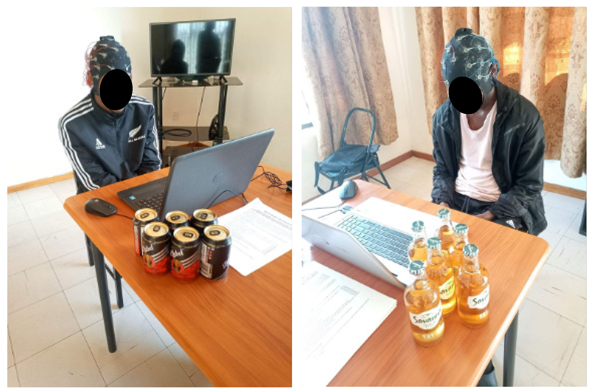
2.1. Data Gathering with Participants

In this work, data were collected from a total of seventeen male alcohol users recruited through oral communication and social media. The study population consisted of male subjects with an age range of 22 to 44 years and a mean age of 27.88 ± 7.08 years. Only individuals with a history of alcohol use were included in the experiments, and alcohol was provided for them to drink during the experiments. Participation in this study was voluntary, and each subject was briefed about the experimental procedure, including eligibility criteria, purpose of the study, privacy, anonymity, and confidentiality. Information on the identity of the participants has been kept confidential and will not be made public. All volunteers had to sign a consent form before taking part in the alcoholism experiments. According to the eligibility criteria as stated in the consent form, any male aged 18 to 60 years with no history of mental illness was allowed to participate in the experiments. At the time of the examination, the volunteers were advised to have very short, dry, and un-oiled hair to increase the contact between the electrodes and the scalp.

To be eligible, the participants had to answer Yes to question 1 and No to questions 2 to 9.

• Have you ever consumed 2 L of 6% alcohol or more in two hours?
• Do you have any alcohol allergies?
• Have you ever had a bad reaction to alcohol?
• Do you suffer from any liver disease?
• Do you suffer from diabetes?
• Do you have any history of diabetes?
• Do you suffer from kidney disease?
• Do you have any history of kidney disease?
• Have you ever been diagnosed with alcohol dehydrogenase deficiency?

Self-Assessment

Each volunteer was given an Alcohol Use Disorder Identification Test (AUDIT) to test their frequency of use of alcohol and their susceptibility to AUD. The AUDIT is a standard screening questionnaire that identifies individuals at risk of alcoholism. This self-report tool comprises 10 questions about possible drinking patterns and the related consequences. The total possible scores for this test range from 0—40, with higher scores showing an increased probability of severe drinking patterns. Possible responses to the questions are within the range of 0—4 except for questions 9 and 10 [23,24]. According to the guidelines set out by the World Health Organization (WHO), a score of 1—7 indicates low-risk alcohol consumption, while a score from 8—14 suggests harmful or hazardous consumption of alcohol. Similarly, scores ranging from 15—40 indicate a likelihood of AUD, that is, moderate to severe AUD. The device used in the experiments was a 32-channel non-invasive EEG wireless headset with a sampling rate of 128 Hz. A gel sensor-based Emotiv Epoc Flex cap was used to record the brain signals of participants under the influence of alcohol. The sensors of the headset were placed following the 10—20 standard electrode placement and the EEG signals were recorded from 32 channels including the following: Cz, Fz, Fp1, F7, F3, FC1, C3, FC5, FT9, T7, TP9, CP5, CP1, P3, P7, O1, Pz, Oz, O2, P8, P4, CP2, CP6, TP10, FC6, C4, FC2, F4, F8, and Fp2, plus two reference sensors. Before commencing the alcohol-drinking experiments, a registered nurse recorded and monitored the vital signs of the volunteers to declare their fitness to participate. All eligible subjects were given a six-pack of alcohol each that contained either 5.5% or 6% of alcohol content, depending on preference. The duration of the experiment was two hours for each volunteer, and the brain signals were recorded throughout the entire period using a non-invasive EEG head module. The rate of consumption was based on the willingness of the volunteer to consume the alcohol, but the timing and estimated amount were confined within two hours. To assist in restraining any possible violent behavior arising from the effects of alcohol on the volunteers, two male security officers were present during the experiments. No adverse side effects were observed in all subjects.

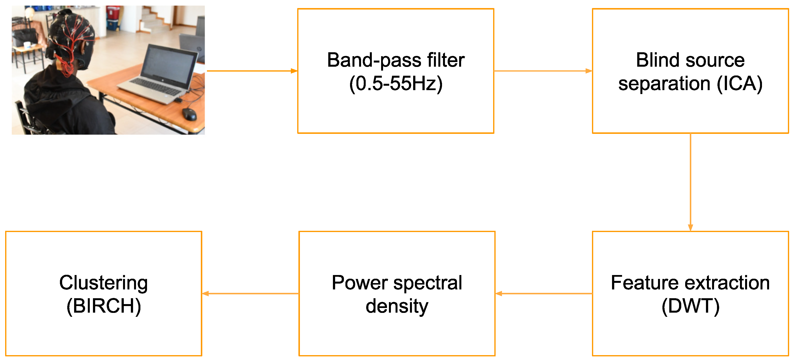
2.2. Data Preprocessing

The study’s raw data harnessed during the alcohol-drinking experiments were first imported in comma-separated variables (CSV) format. Filtering was applied using notch and band-pass filters to remove artifacts in the data. The data were then segmented into 20-min intervals for epoching and creating fixed-length events. ICA was used to separate independent components from the raw data using the MNE open-source Python 3.10 package [25]. Finally, DWT was applied to decompose the ICA-processed data into time—frequency domain features.

2.2.1. Importing Raw Data

The initial step in the EEG analysis was importing the raw data recorded during the experiments. There are different types of EEG data storage, such as Functional Imaging File (FIF), European Data Format (EDF), and CSV. In our study, we used the CSV format because it allows for easier manipulation and analysis of brain signals.

2.2.2. Filtering

To reduce physiological and non-physiological artifacts and improve the quality of the data, we implemented notch and band-pass filters. Brain signals are usually affected by power line noise at 50 or 60 Hz, depending on the region [26]. To remove this electrical interference, a notch filter was implemented in the data with a cutoff frequency of 60 Hz. The second artifact removal step was a band-pass filter that was implemented within the range of 0.5 to 55 Hz. This type of filter allowed us to isolate the delta (0.5—4 Hz), theta (4—8 Hz), alpha (8—12 Hz), beta (12—35 Hz), and gamma (35—55 Hz) brain rhythms to enhance the signal-to-noise ratio of the data [27].

A band-pass filter of 0.5—55 Hz was used in this study because we wanted to maintain information from the EEG frequency bands including delta (0.5—4 Hz), theta (4—8 Hz), alpha (8—12 Hz), beta (12—35 Hz), and gamma (35—55 Hz). The upper band of 55 Hz ensured that the power line noise was removed from the signals and the strong oscillatory artifacts that occur at those frequencies [28,29]. This study focuses on the analysis of the theta, alpha, and beta frequency bands, and therefore, the use of the 55 Hz upper band does not have any significant impact on the analysis of this paper. This is because, based on the related literature, the delta band is often influenced by non-neural artifacts, such as slow eye movements and drowsiness, while the gamma band is influenced especially in awake and task-free EEG recordings [30,31]. In contrast, theta, alpha, and beta bands are more reliably associated with cognitive control, attention, and inhibitory process functions, which are directly affected by alcohol use [32,33]. These bands also provide more robust and interpretable features for AUD analysis.

2.2.3. Epoching

This step involves creating time-locked data segments called epochs. In our study, we wanted to observe the transitions that occur in the brain when a person drinks alcohol. The EEG data were recorded continuously for a total of two hours during the drinking session, and the data were segmented into six epochs of 20 min each. Each epoch corresponds to the approximate consumption of one bottle of alcohol, as participants were provided with a six-pack and consumed one bottle per 20 min interval. According to [34], using longer EEG windows (10—20 min) enhances classification performance and the reliability of EEG-derived metrics. This longer duration may provide a more stable representation of brain states and improve the detection of significant transitions.

2.2.4. ICA

This is one of the most prominent blind source separation techniques in which independent components are estimated from a set of EEG recordings. Mixed signals, such as eye blinks and muscle movement, are removed to ensure that analysis of the EEG data is independent of external interference [26,35]. ICA provides a more artifact-free characterization of the brain by eliminating undesired segments from the original signal [36].

2.2.5. Discrete Wavelet Transform

Due to the non-linearity and non-stationary properties of the EEG signals, the extraction of the relevant features needed for analysis may be complex [37]. A more robust method is needed to achieve accuracy in extracting informative characteristics of the data. Therefore, DWT has been proposed in this work to decompose the signals into highly efficient representations called wavelets. This technique helps in capturing useful time—frequency domain features of the data at different resolutions [38,39].

2.3. Data Presentation

Due to there being a lot of redundant information in high-dimensional data, the dimensionality reduction method can be utilized to convert them from a high- to low-dimensional feature space [40]. In our study, we implemented the PCA technique to perform this, which is a technique that aims to find the optimal variance from a set of features. These are transformed into smaller features that contain the most information about the data. It also reduces the complexity of a model while improving its efficiency. In the case of duplicate features, PCA can overcome this, as it creates a new set of non-linearly related features [41]. We applied PCA to the DWT-processed data by defining two principal components to plot our clustering results in two-dimensional feature space. We used clustering after PCA, which is an unsupervised learning technique where a set of unlabeled data is analyzed based on the data correlations. Many different algorithms can be applied, which are dependent on the type and size of the dataset [42]. In this work, the BIRCH method was used, which is a hierarchical clustering method that creates a tree-like structure using clustering features (CFs) and a cluster feature tree (CF Tree). It is memory-efficient and can handle large datasets with a faster execution time [19,42].

3. Results and Discussion

In this section, we present three main types of results derived from the processing of our data. We start with the analysis of the spectral power of the theta, alpha, and beta frequency rhythms for low-risk consumption, harmful or hazardous consumption, and a likelihood of AUD. We then discuss the transitions of the brain signals at the first and last moments of alcohol intake. Finally, we describe the overall cluster results for all the participants combined by showing the brain activity of the subjects with hazardous alcohol use, dependence symptoms, and lastly those with severe alcohol use to analyze the severity level of AUD.

3.1. Power Spectral Density Analysis

In the following paragraphs, we present the PSD graphs for participants from each category of low-risk consumption, harmful or hazardous consumption, and a likelihood of AUD, based on the individual responses of the AUDIT. From each category of low-risk consumption, harmful or hazardous consumption, and a likelihood of AUD, we chose one subject (of the total 17) that had satisfied the highest number of consumption criteria based on the AUDIT scores. We present the theta, alpha, and beta frequency band results during the first and last phases of alcohol intake.

3.1.1. Theta Band

This frequency rhythm lies within the range (4—8 Hz) and is mostly responsible for the regulation of learning, inhibitory control processes, and intuition. It is generated across all parts of the cortex and acts as a repository for memories and emotions [43].

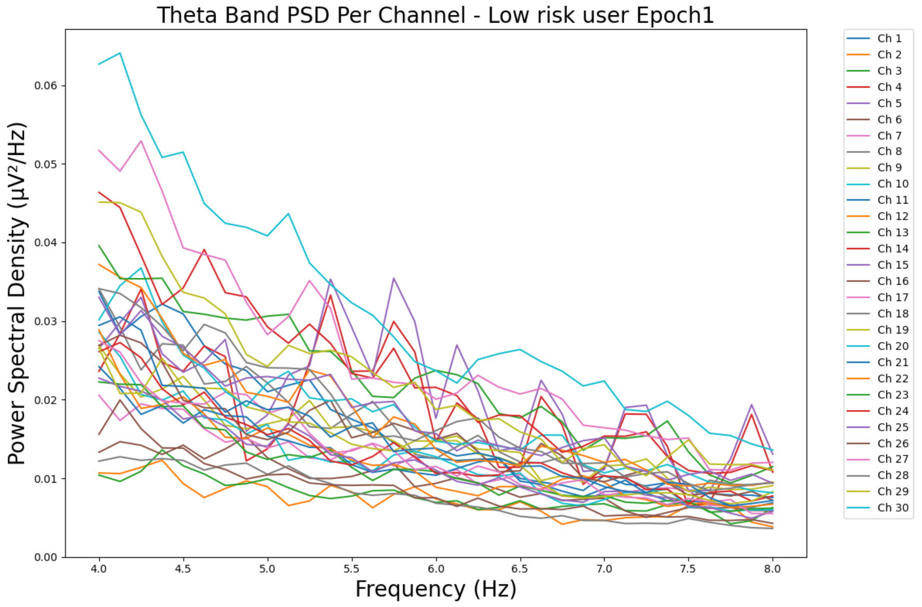
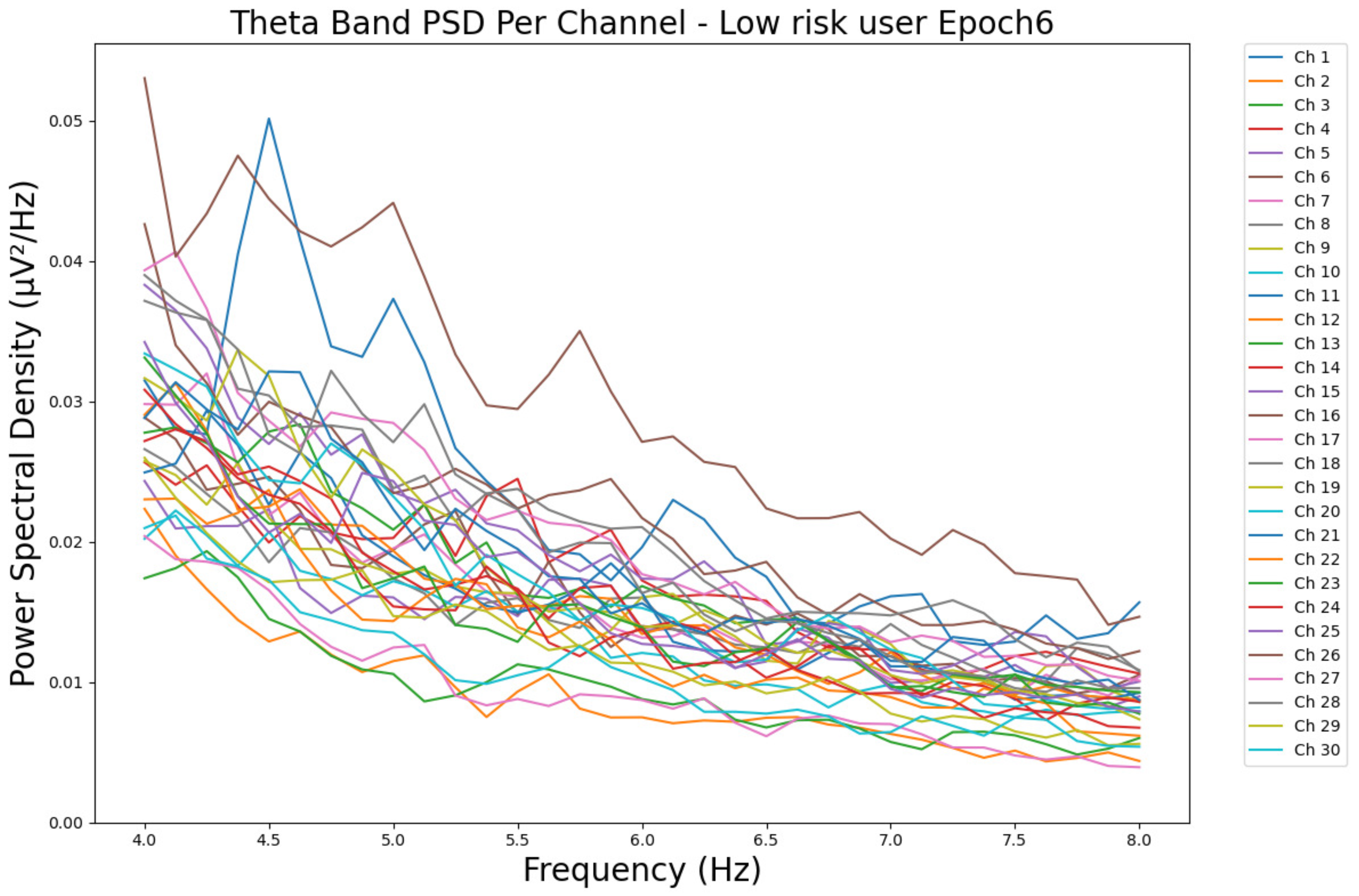
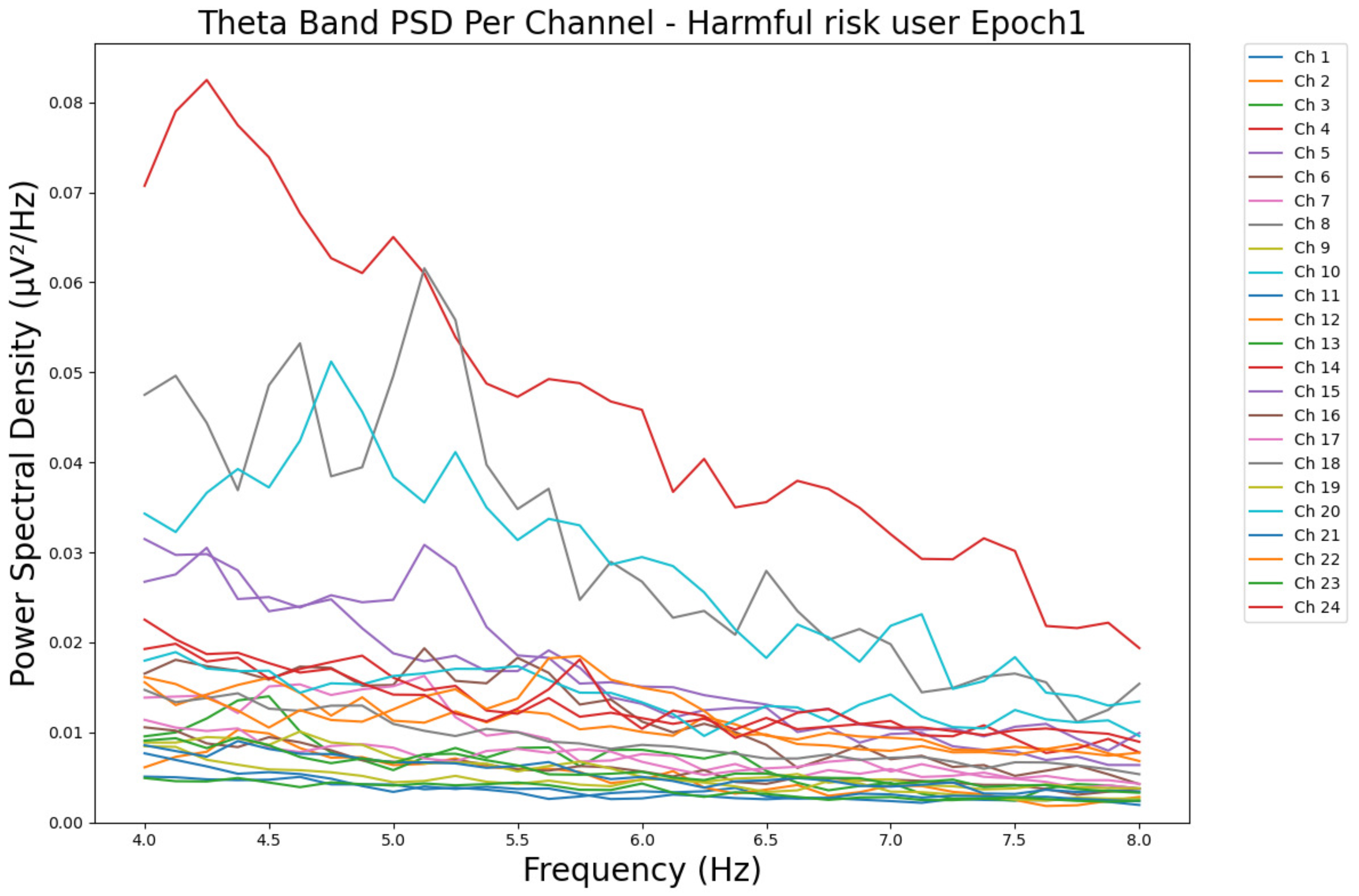
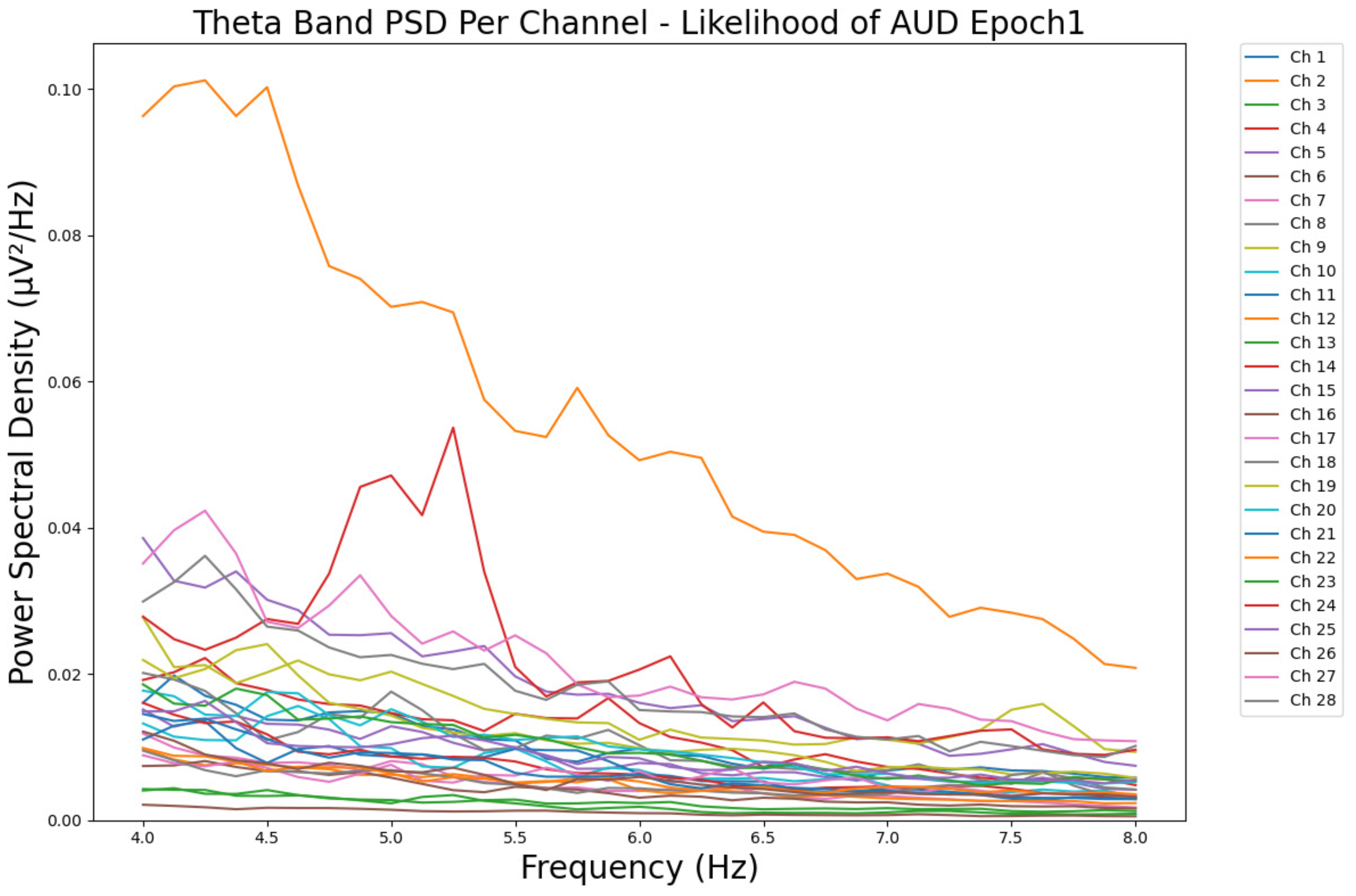
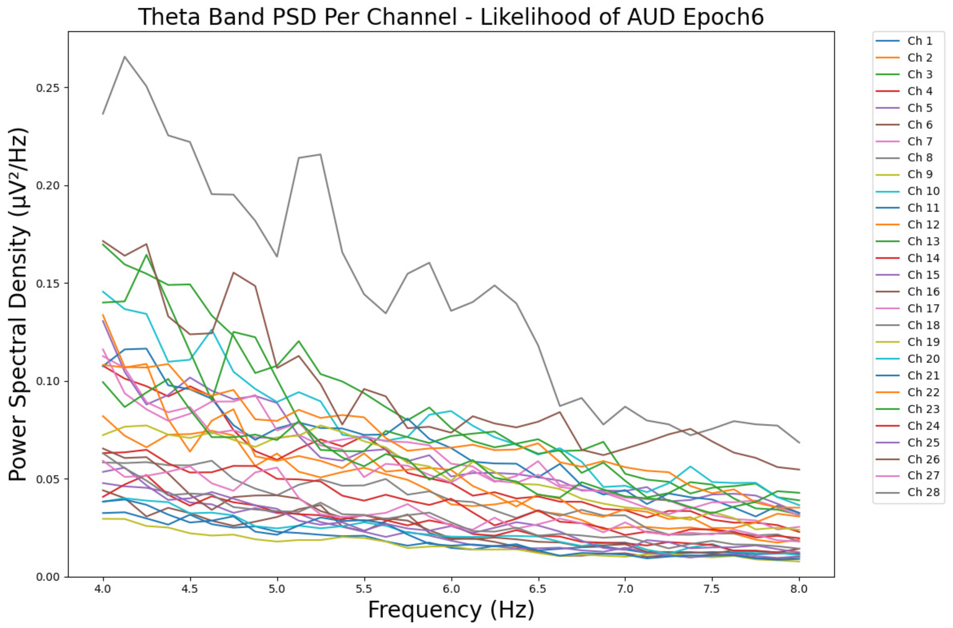
• Observations
  We can observe the PSD of a low-risk consumer ranging from 0.005 to 0.065 μV²/Hz in Figure 3 and from 0.005 to 0.055 μV²/Hz in Figure 4. We can also observe the PSD of a harmful or hazardous consumer ranging from 0.005 to 0.09 μV²/Hz in Figure 5 and from 0.005 to 0.15 μV²/Hz in Figure 6. Finally, we can observe the PSD of a participant with a likelihood of AUD ranging from 0.00 to 0.10 μV²/Hz in Figure 7 and from 0.001 to 0.28 μV²/Hz in Figure 8. The participant with low-risk consumption has a higher degree of signal entanglement in epoch 1, followed by the one with harmful or hazardous consumption, and lastly, the subject with a likelihood of AUD. On the contrary, in epoch 6, we can observe a higher degree of signal entanglement for the harmful consumer, followed by the one with low-risk consumption, and lastly, the subject with a likelihood of AUD. Based on these results, during the first phase of alcohol intake, the participant with a likelihood of AUD has the highest range of theta power, followed by the harmful consumer, and lastly, the low-risk consumer. Similarly, during the last phase of alcohol intake, the subject with the likelihood of AUD has the highest range of theta power, followed by the harmful or hazardous consumer and then the low-risk consumer.
• Interpretations
  In general, for the theta band, more alcohol consumption results in more spectral power. This is true for all types of alcohol consumption. However, for people with a smaller frequency of consumption, the level of activation is much higher compared to the highest frequency of consumption. For the data gathered in this experiment, the highest frequency of consumption has five times more spectral power than the lowest frequency of consumption. This means that people with higher alcohol consumption are more coherent in their level of concentration and thus that they tend to be more functional in performing normal tasks compared to those with lower consumption. The high degree of signal entanglement results from the activation of inhibitory and motor responses caused by alcohol consumption as these are regulated by the theta band [43]. The level of activation is much higher for people with a smaller frequency of use because they project more acute performance impairment symptoms due to higher alcohol consumption. In most people, mild intoxication can be observed after two standard drinks [7].

3.1.2. Alpha Band

The alpha band is a state of the brain that predominates through the resting state and enhances an individual’s relaxation of their mental state. Its frequency ranges between 8 and 12 Hz and it is responsible for mental coordination and consciousness that does not involve any cognitive tasks. Its power spectrum has been proven to be mostly suppressed during body activities with eyes wide open [44].

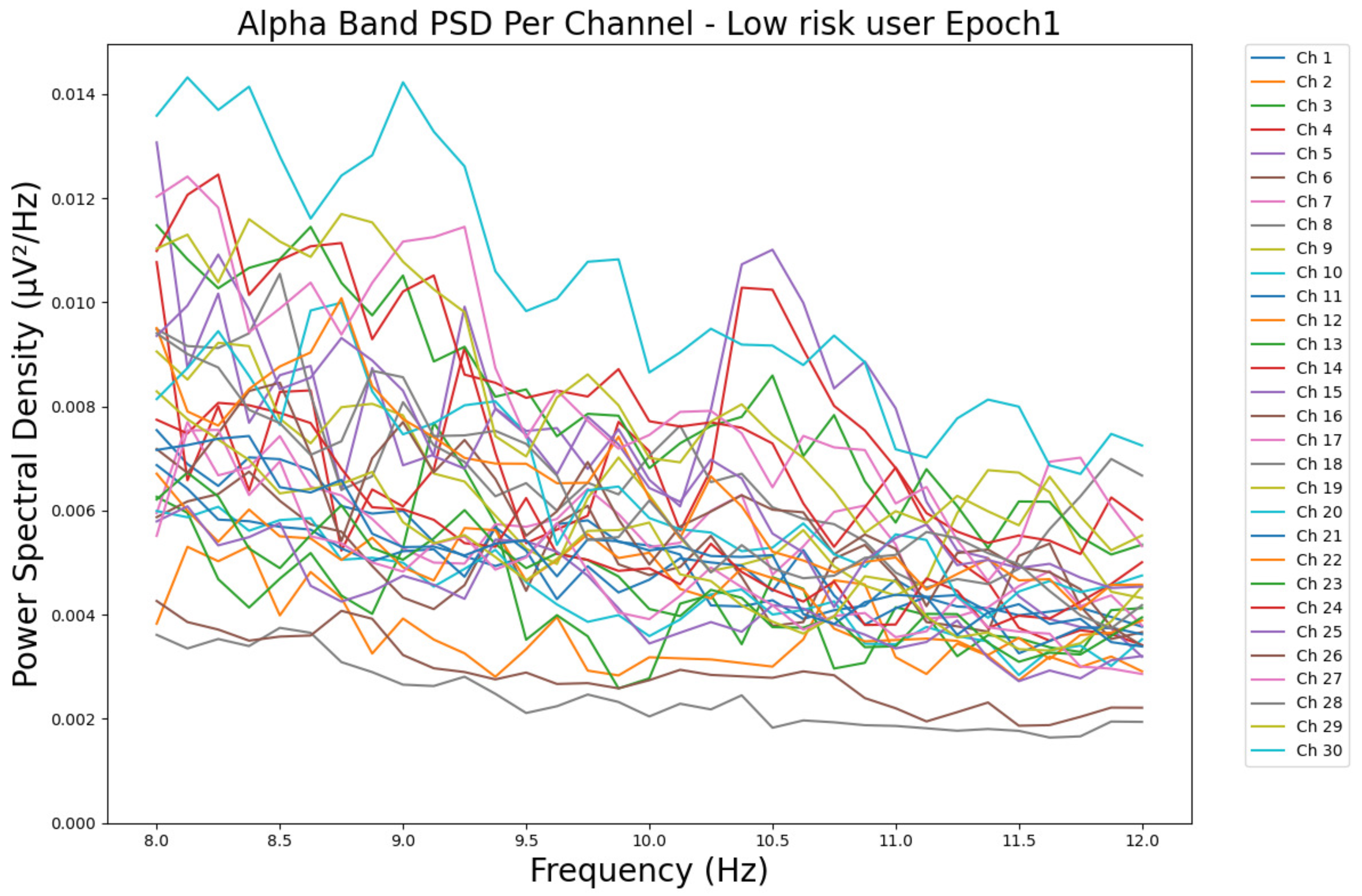
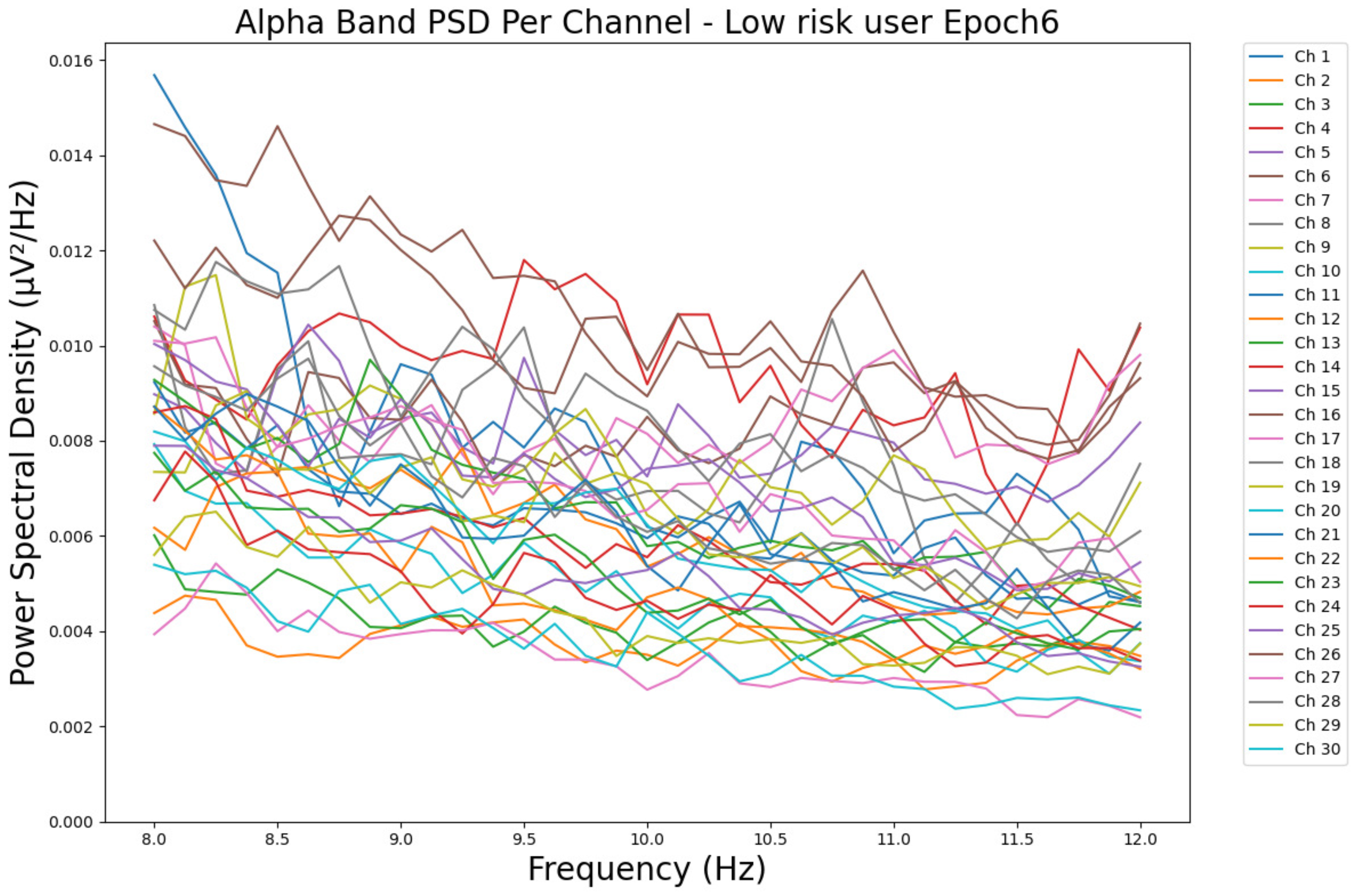
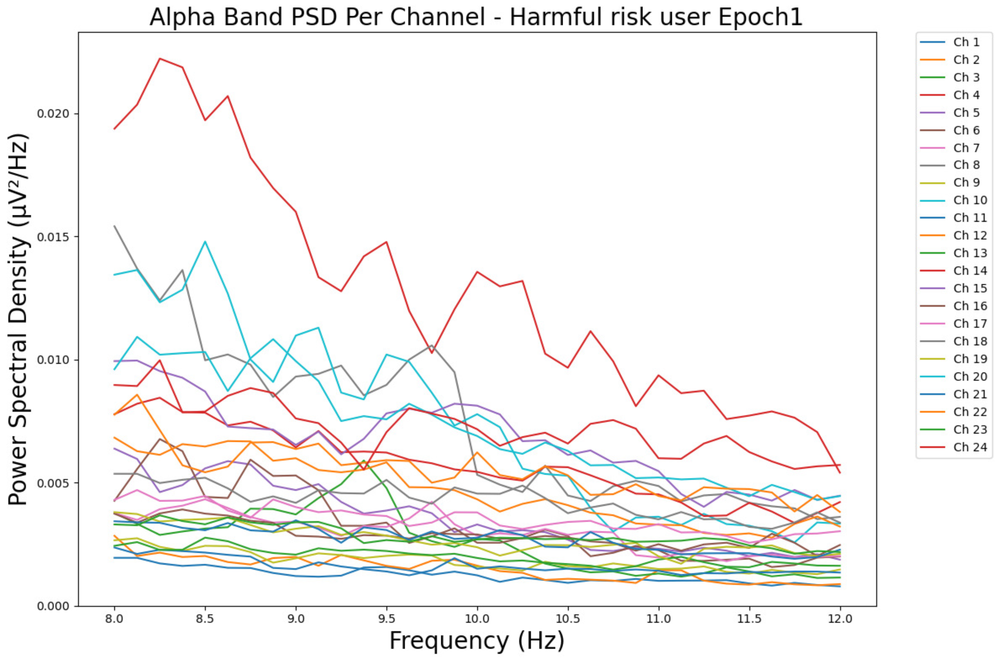
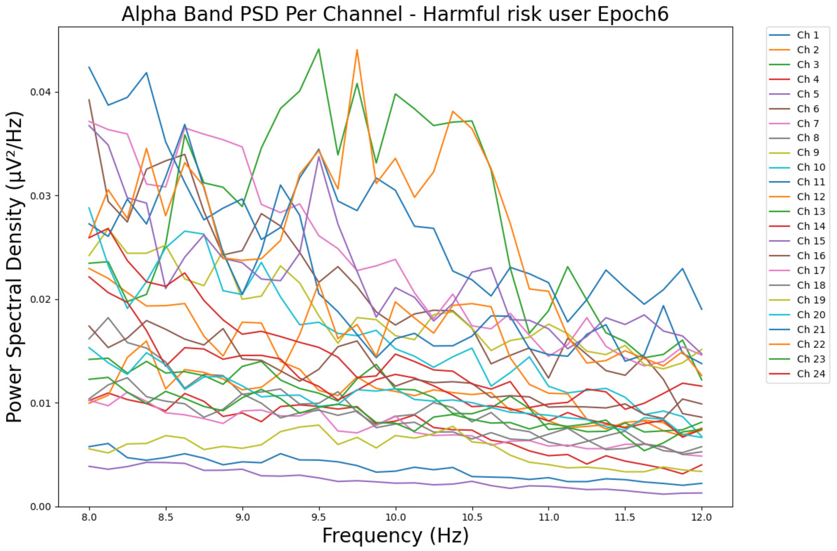
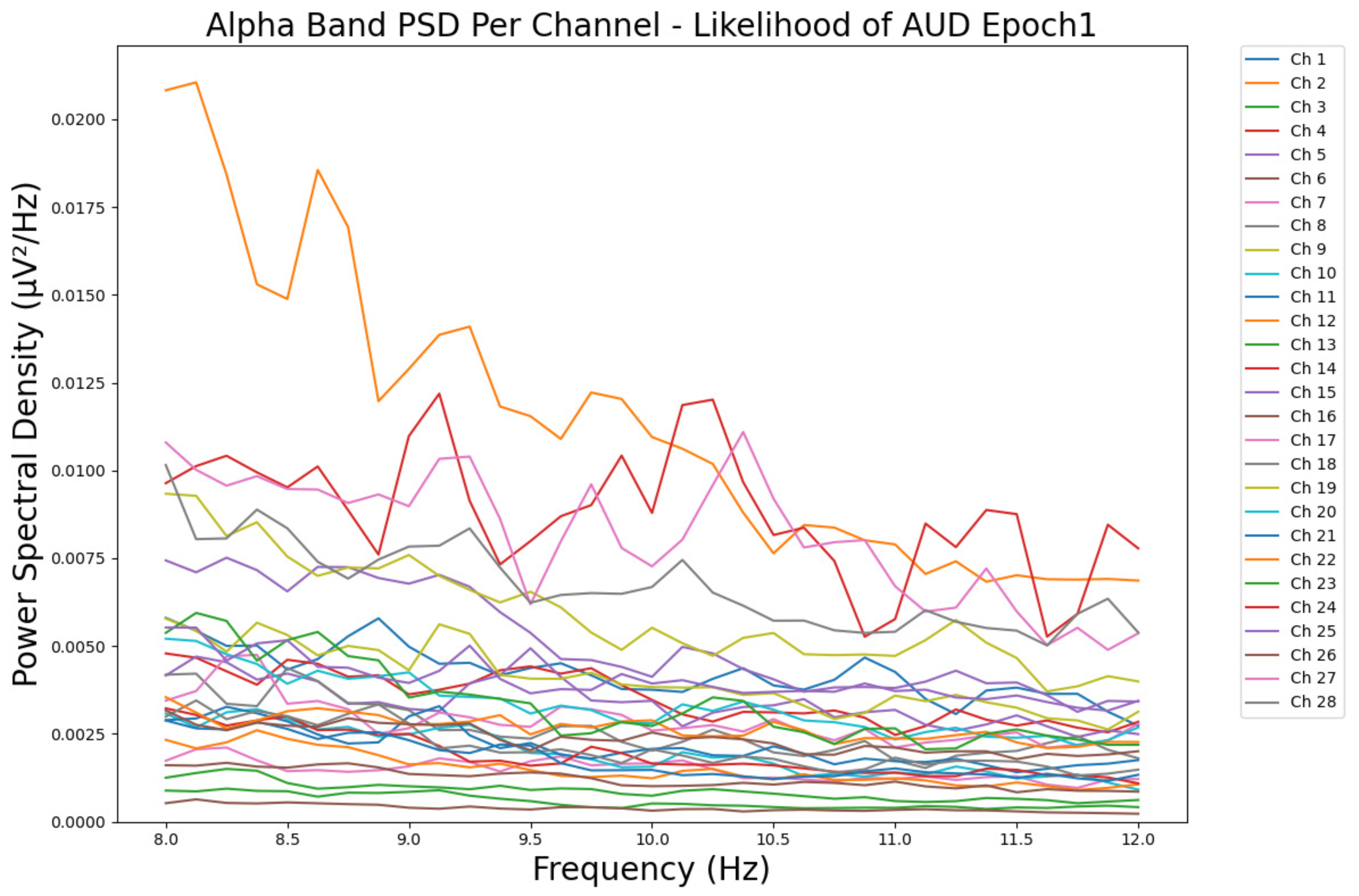
• Observations
  Compared to the results of the theta band, we can observe a significant decrease in alpha in the range of the PSD for all the subjects in all the epochs. Although the results of the alpha band are smaller than theta, there is an increase in the average PSD between epochs 1 and 6 for all three types of consumption. We can observe the PSD of a low-risk consumer ranging from 0.002 to 0.014 μV²/Hz in Figure 9 and from 0.002 to 0.0158 μV²/Hz in Figure 10. The PSD for a harmful or hazardous consumer in Figure 11 ranges from 0.002 to 0.024 μV²/Hz and from 0.005 to 0.48 μV²/Hz in Figure 12. Lastly, the PSD for an individual with a likelihood of AUD in Figure 13 ranges from approximately 0.000 to 0.0225 μV²/Hz in epoch 1 and from 0.005 to 0.075 μV²/Hz in Figure 14. Similar to the theta band, we can observe a higher degree of signal entanglement for the subject with low-risk consumption, followed by the harmful or hazardous consumer, and lastly, for the subject with a likelihood of AUD in epoch 1. For epoch 6, we can observe a higher degree of signal entanglement in the subject with harmful or hazardous consumption, followed by the low-risk consumer, and lastly, the one with a likelihood of AUD.
• Interpretations
  In the alpha band, the same trend of activation is observed as in the theta band. However, the value of the spectral power is smaller because it is mostly suppressed during body activities with eyes wide open. A higher alpha power is more prominent in the resting state, and thus, more alcohol consumption results in less relaxation and more agitation [44]. People with lower alcohol consumption can be easily disturbed by outside stimuli compared with people with higher consumption, as they can be calmer. Increasing the amount of alcohol consumption results in cortical activations and alert mechanisms and thus causes less relaxation [45].

3.1.3. Beta Band

In the beta rhythm, the frequency ranges from 12 and 35 Hz, which can further be subdivided into low beta (12—15 Hz), mid beta (15—18 Hz), and high beta (above 18 Hz). It is a state of the brain in which sensory—motor control tasks are processed and it occurs during information processing, decision-making, and problem-solving. It is recorded in the frontal regions of the brain [46].

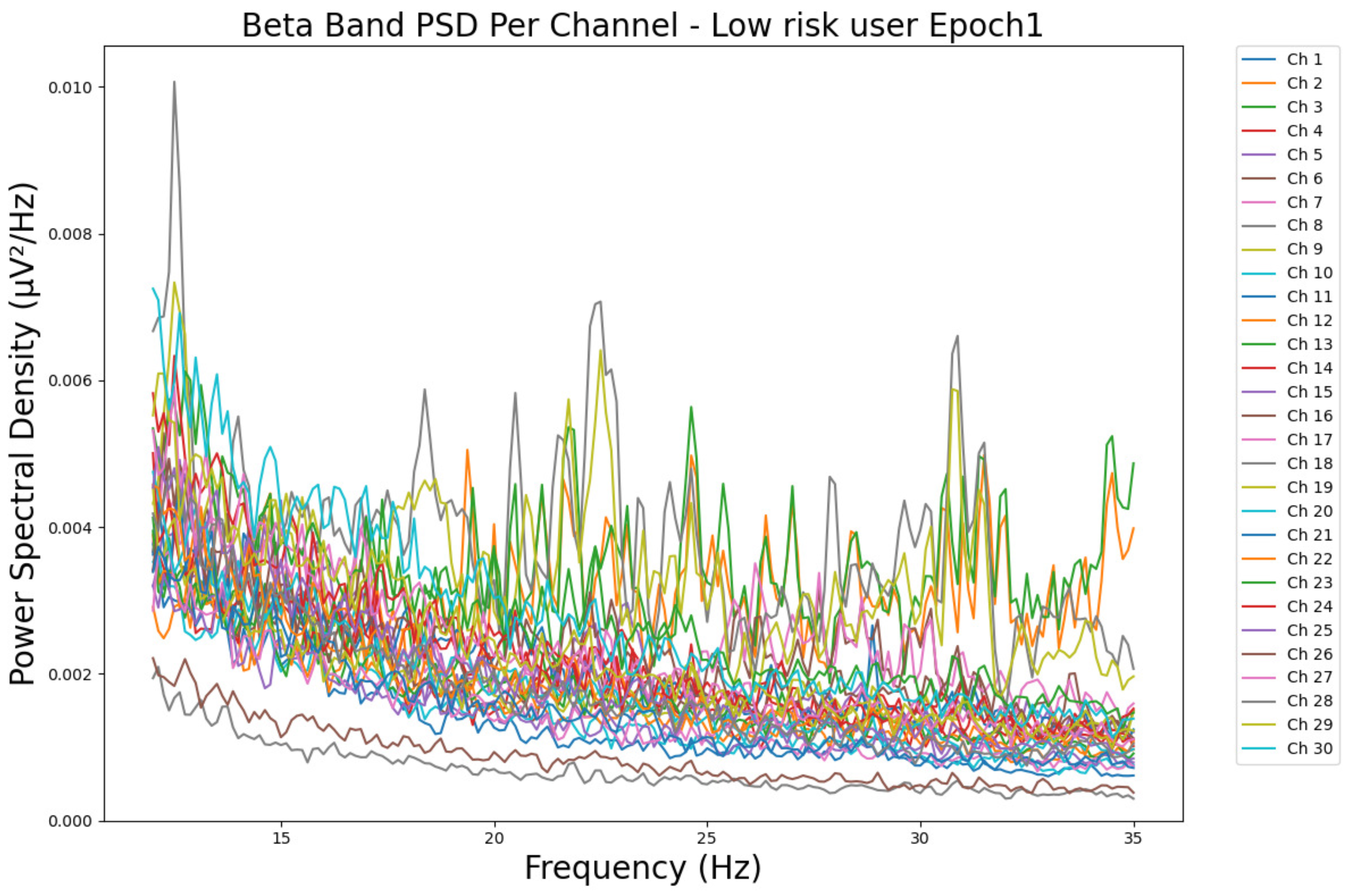
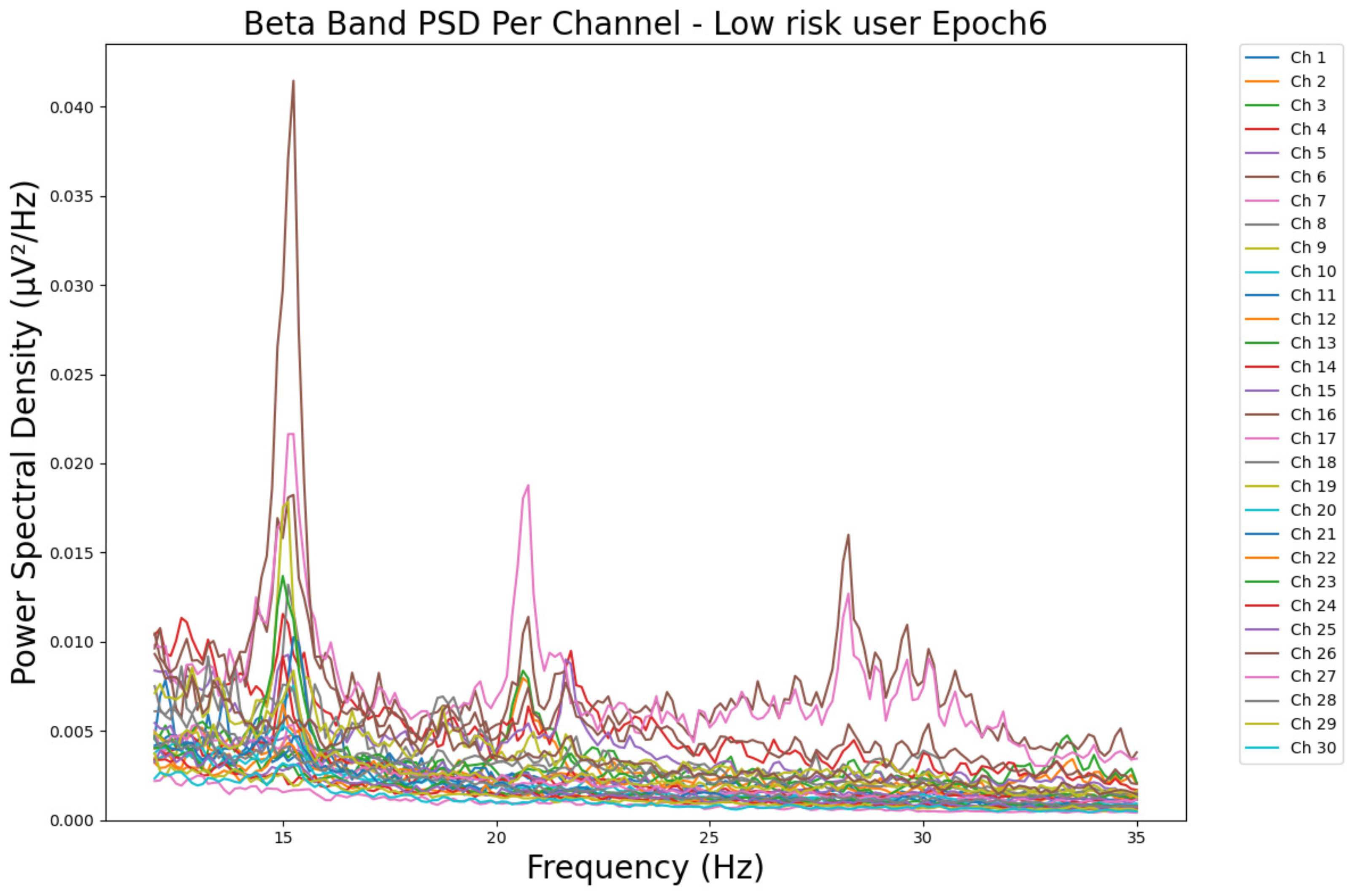
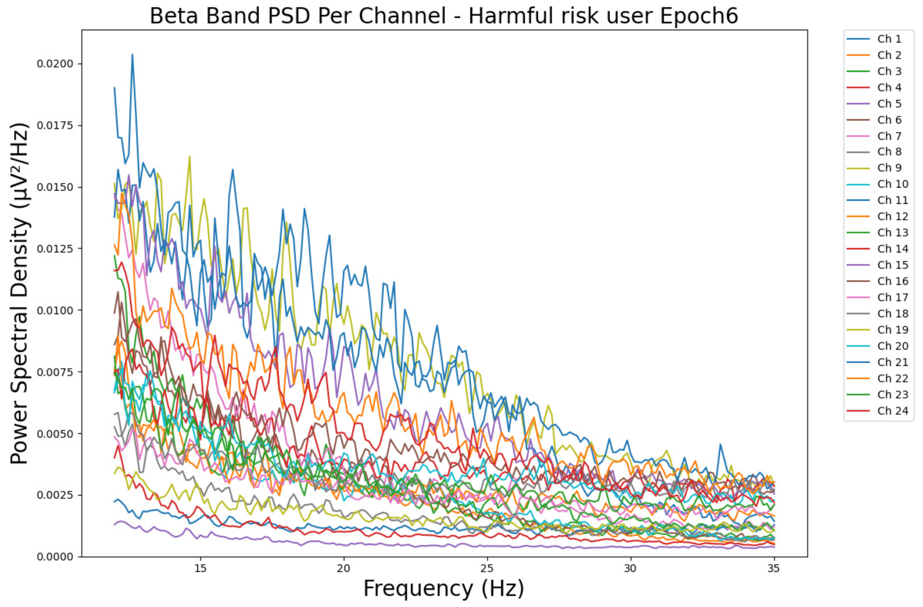
• Observations
  The PSD of a low-risk consumer ranges from 0.0005 to 0.01 μV²/Hz in Figure 15 and from 0.000 to 0.045 μV²/Hz in Figure 16. For a harmful or hazardous consumer in Figure 17, the PSD ranges from approximately 0.000 to 0.0065 μV²/Hz and approximately 0.000 to 0.02 μV²/Hz in Figure 18. Lastly, the PSD for the subject with a likelihood of AUD in Figure 19 ranges from 0.000 to 0.013 μV²/Hz and from 0.000 to 0.024 μV²/Hz in Figure 20. The signals appear to fluctuate independently, but the degree of signal entanglement is more significant in the low-risk consumer, followed by the harmful or hazardous consumer, and lastly, the subject with a likelihood of AUD. We can also observe that some signals have peaks at certain frequencies, with the low-risk consumer having more pronounced peaks, followed by the harmful consumer, and lastly, the subject with a likelihood of AUD in epoch 1. In epoch 6 of the low-risk consumer, we can observe a significant peak at 15 Hz.
• Interpretations

Similar to the theta and alpha bands, the beta band has more spectral power for a higher frequency of alcohol compared to lower alcohol consumption. This is because beta is about focus and concentration; thus, the person with the least alcohol consumption has less motor control relative to the same amount of consumed alcohol compared to the person with the highest frequency of consumption.

The spectral power of the low-risk consumer is more pronounced and significant in the sensory—motor rhythm (12—15 Hz). This rise in beta power may indicate an imbalance between the excitatory and inhibitory neural responses resulting from increasing alcohol amount for an individual whose consumption is low [47]. A study by [48,49] suggests that an increase in beta spectral power is normally produced before developing AUD. In our results, the PSD in the beta band was generally lower than the theta and alpha rhythms. This may be evidence of AUD vulnerability when the frequency of consumption is increased. We can say that the subjects are projecting symptoms of AUD due to the increasing alcohol amount but do not necessarily suffer from AUD. Additionally, the increase in the beta spectral power does not entirely depend on the rate and frequency of use of alcohol. As such, the possibility of the subjects being alcohol-dependent is reduced because the increase of the beta power may be related to a family history of AUD [10]. This further supports our argument that the subjects in the study may be prone to AUD if they increase their frequency of alcohol consumption. Lastly, the pronounced peaks observed in the beta results may indicate personality traits associated with the risk of developing AUD because results in beta have been considered a trait marker according to [48,50,51]. This is to say that the beta spectral power can be used to diagnose potential endophenotypes that put individuals at risk of developing AUD before the presence of symptoms. In epoch 1, lower-risk participants exhibit more dispersed and variable EEG patterns, which likely reflects increased cognitive response or lower tolerance, while in epoch 6, higher consumption groups show denser, more centralized clusters, suggesting potential composure for the same amount of alcohol consumed. These transitions align with increased spectral power in theta and beta bands and are consistent with the previous literature on neural habituation and alcohol-related EEG markers.

In general, a person with a smaller frequency of alcohol consumption is greatly affected by the effects of alcohol for the same amount of alcohol consumed compared to a person with a higher frequency of consumption. This can hinder their ability to make proper judgments and informed decisions, leading to impaired motor coordination [52]. Results in theta have the highest PSD across all the subjects compared to the other two bands because a study by [48] suggests that theta is considered a state marker in alcoholism. This means that the spectral power of the theta band can be used as a biomarker to diagnose the presence of AUD. According to [10], the spectral power in EEG can be used to examine the extent of alcohol use by showing neural changes associated with its consumption. The results in the theta, alpha, and beta bands can correlate with the severity of AUD and how it affects the brain.

Figure 15. Epoch 1 represents the initial phase of alcohol for low-risk consumption in the beta band and with a PSG range of 0.0095 μV²/Hz.

Figure 15. Epoch 1 represents the initial phase of alcohol for low-risk consumption in the beta band and with a PSG range of 0.0095 μV²/Hz.

Figure 16. Epoch 6 represents the last phase of alcohol intake for low-risk consumption in the beta band with the PSD range increased by 0.035 μV²/Hz.

Figure 16. Epoch 6 represents the last phase of alcohol intake for low-risk consumption in the beta band with the PSD range increased by 0.035 μV²/Hz.

Figure 17. Epoch 1 represents the initial phase of alcohol for harmful or hazardous consumption in the beta band with a range of 0.065 μV²/Hz.

Figure 17. Epoch 1 represents the initial phase of alcohol for harmful or hazardous consumption in the beta band with a range of 0.065 μV²/Hz.

Figure 18. Epoch 6 represents the last phase of alcohol intake for harmful or hazardous consumption in the beta band with the PSD range increased by 0.0135 μV²/Hz.

Figure 18. Epoch 6 represents the last phase of alcohol intake for harmful or hazardous consumption in the beta band with the PSD range increased by 0.0135 μV²/Hz.

Figure 19. Epoch 1 represents the initial phase of alcohol intake for likelihood of AUD in the beta band and with a PSD range of 0.013 μV²/Hz.

Figure 19. Epoch 1 represents the initial phase of alcohol intake for likelihood of AUD in the beta band and with a PSD range of 0.013 μV²/Hz.

Figure 20. Epoch 6 represents the last phase of alcohol intake for likelihood of AUD in the beta band with the PSD range increased by 0.011 μV²/Hz.

Figure 20. Epoch 6 represents the last phase of alcohol intake for likelihood of AUD in the beta band with the PSD range increased by 0.011 μV²/Hz.

Statistically, one-way ANOVA revealed significant differences across the groups: low-risk consumption, harmful or hazardous risk consumption, and likelihood of AUD in all frequency bands and epochs. The theta band in epoch 1 had the strongest group separation (F = 14.23, p = 0.0047), supporting the notion that it is a potential state marker for AUD. The ANOVA results are presented in

Table 2. ANOVA results on EEG band power across alcohol consumption groups.

Frequency Band	Epoch	Low-Risk	Hazardous	AUD	F-Stat	p-Value
Theta	1	2.10	1.82	2.05	14.23	0.0047
Theta	6	2.25	1.90	2.30	12.81	0.0085
Alpha	1	1.10	1.20	0.95	10.75	0.0123
Alpha	6	1.20	1.18	1.10	9.54	0.0196
Beta	1	0.95	0.85	0.80	7.62	0.0251
Beta	6	0.97	0.90	0.85	6.38	0.0320

, which shows both mean PSD values per group and the associated ANOVA F-statistics and p-values. All frequency bands showed statistically significant group differences (p < 0.05). Notably, the theta band at epoch 1 demonstrated the highest F-statistic (14.23), consistent with its known sensitivity to alcohol’s acute cognitive effects. Additionally, we present the mean, standard deviation, and confidence intervals in

Table 3. Statistical analysis of PSD results (in μV²/Hz) across epochs and consumption groups.

Frequency Band	Epoch	Group	Mean	Std Dev	95% CI
Theta	1	Low-risk	0.0156	0.0089	±0.0006
		Hazardous	0.0120	0.0117	±0.0008
		AUD	0.0107	0.0120	±0.0008
	6	Low-risk	0.0163	0.0078	±0.0005
		Hazardous	0.0422	0.0286	±0.0020
		AUD	0.0501	0.0367	±0.0024
Alpha	1	Low-risk	0.0058	0.0023	±0.0001
		Hazardous	0.0043	0.0032	±0.0002
		AUD	0.0035	0.0028	±0.0002
	6	Low-risk	0.0065	0.0023	±0.0001
		Hazardous	0.0143	0.0088	±0.0006
		AUD	0.0157	0.0100	±0.0006
Beta	1	Low-risk	0.0021	0.0011	±0.0000
		Hazardous	0.0014	0.0009	±0.0000
		AUD	0.0013	±0.0000	±0.0000
	6	Low-risk	0.0029	0.0024	±0.0001
		Hazardous	0.0037	0.0030	±0.0001
		AUD	0.0040	0.0033	±0.0001

for the PSD results. In general, Table 3 shows that more alcohol consumption results in more spectral power. This is because across all the frequency bands, an increase in PSD can be observed from epochs 1 to 6. In addition, results in the theta band have the highest spectral power compared to the alpha and beta rhythms. These confirm our interpretations from the PSD graphs.

3.2. Transition-Based Clustering Results

In the following paragraphs, we discuss the transitions of the brain signals from the initial to the final phase of alcohol intake for low-risk consumption, harmful or hazardous consumption, and likelihood of AUD. These transitions will be used to understand an individual’s cognitive and behavioral changes with increasing alcohol amount. The results of epoch 1 represent the initial phase of alcohol intake, while those for epoch 6 represent the last phase of alcohol intake. We discuss the observations of epoch 1 followed by epoch 6.

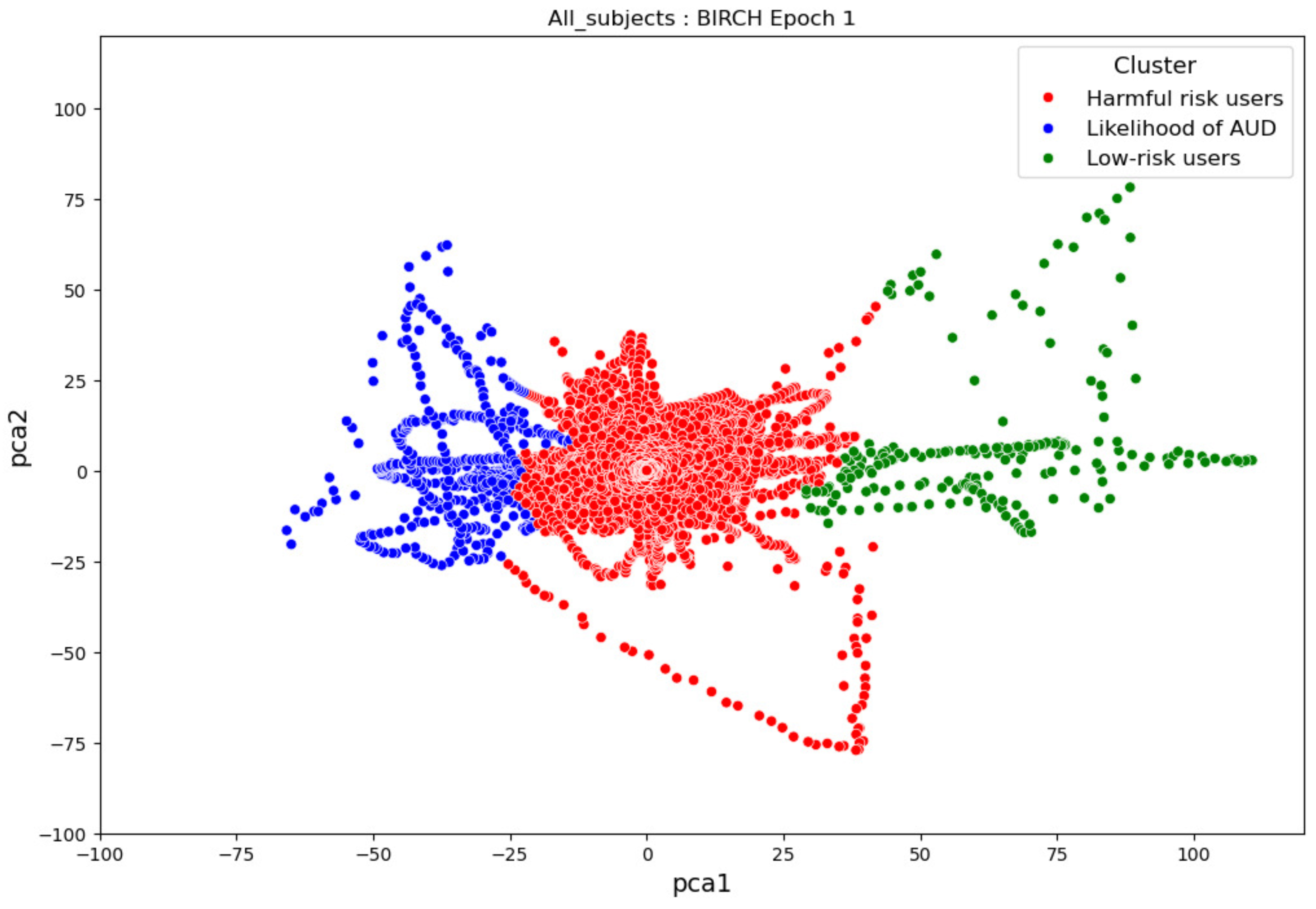
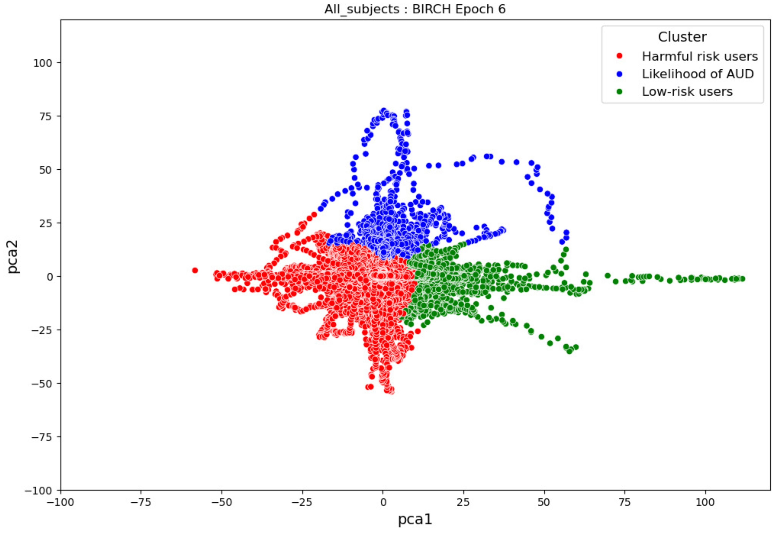
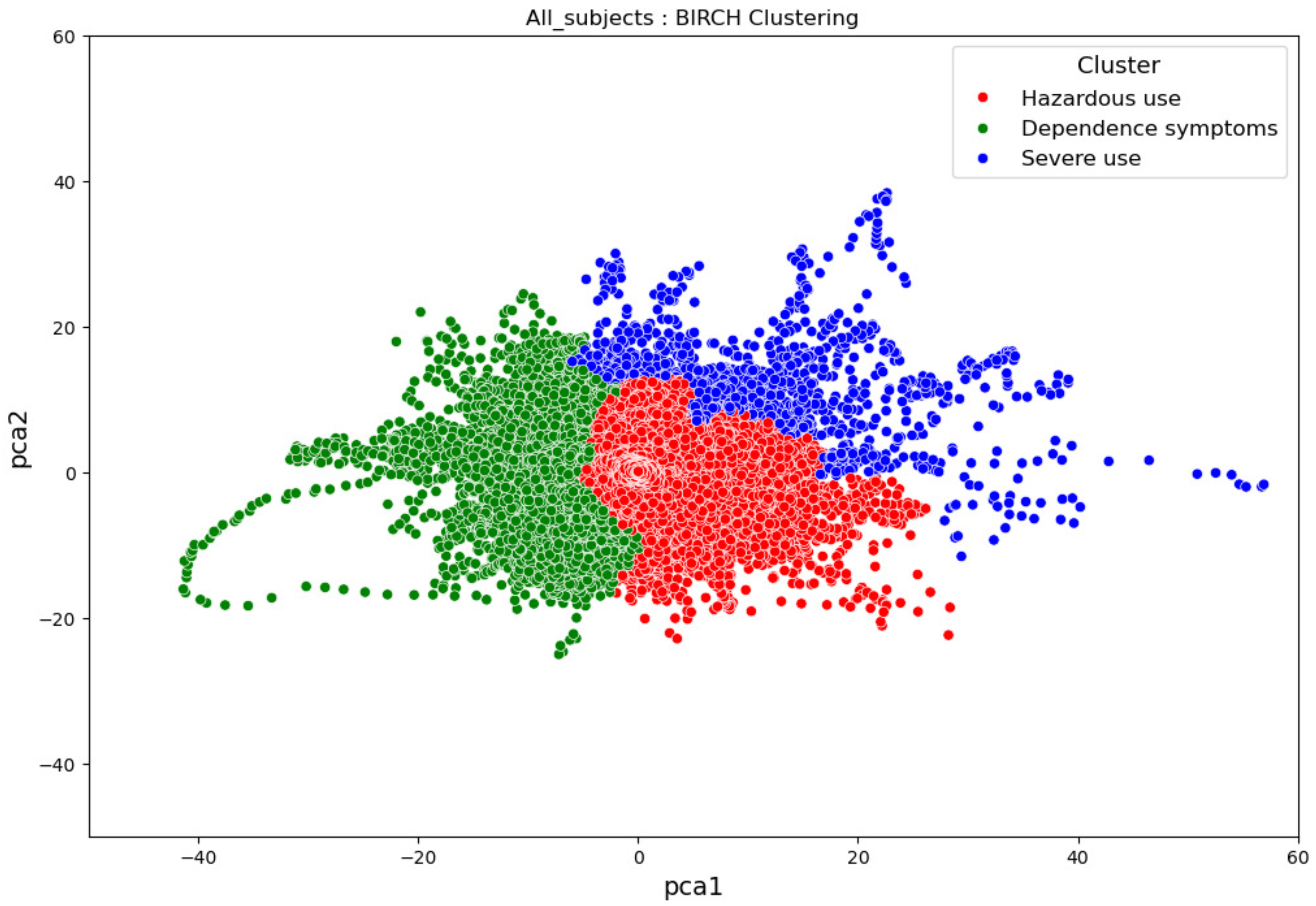
• Observations
  In Figure 21, the clustering results indicate the three major clusters that represent the brain activity of participants at the first instance of alcohol intake. We can observe more dispersed data points for the green cluster, followed by the red cluster, and lastly, the blue cluster. The red cluster is more dense than the blue and green clusters and covers a wider range than the other two. The data points in the red cluster fall between the blue and the green clusters. In Figure 22, we can also observe three major clusters that represent the brain signals of participants at the last instance of alcohol intake. Compared to the epoch 1 cluster results, the data points are more confined and less dispersed. We can also observe that the data points in the blue and green clusters intersect with the larger values of the PCA1 axis. Similarly, some data points in the green cluster overshoot towards the larger values of the PCA1 axis.
• Interpretations
  The three major clusters in Figure 21 and Figure 22 represent the brain activity of people with low-risk alcohol consumption, hazardous or harmful alcohol consumption, and a likelihood of AUD. The blue cluster in Figure 21 represents the brain activity of people with a likelihood of AUD, the red cluster represents those with harmful or hazardous consumption, and lastly, the green cluster represents those with low-risk consumption. The dispersion of the data points in Figure 21 indicates the neurophysiological changes and the brain activation induced by alcohol consumption. In addition, individuals experience more brain activation and a higher degree of signal entanglement for lower alcohol consumption compared to higher alcohol consumption. The brain activities of people with low-risk consumption and a likelihood of AUD in Figure 22 intersect because according to [53], these consumers may project similar characteristics during binge drinking. The data overshoot in Figure 22 of the green cluster indicates the higher spectral power that is mostly associated with the activation of the inhibitory and motor responses caused by increasing amounts of alcohol for individuals with low consumption. An increase in alcohol consumption causes an increase in the spectral power of the theta, alpha, and beta frequency bands. Lastly, the brain activity of people who have moderate to high alcohol consumption indicates less motor control impairment compared to those with low-risk consumption [53] and thus is calmer for the same amount of alcohol consumption.

3.3. Overall Clustering Results

For our overall clustering results in Figure 23, we implemented the BIRCH algorithm. We obtained a maximum of three clusters that represent hazardous alcohol use, dependence symptoms, and severe alcohol use as a result of increasing alcohol consumption. The total number of scores recorded by the 17 participants in the three AUDIT domains are presented in

Table 4. The three domains of the AUDIT with the total responses recorded from the 17 participants in the alcoholism experiments.

Domains	Questions	Item Content	Responses
Hazardous alcohol use	1	Frequency of drinking	31
	2	Typical quantity	45
	3	Frequency of heavy drinking	38
Dependence symptoms	4	Impaired control over drinking	21
	5	Increased salience of drinking	13
	6	Morning drinking	25
Severe alcohol use	7	Guilt after drinking	28
	8	Blackouts	28
	9	Alcohol-related injuries	9
	10	Others concerned about drinking	14

. In this table, the last domain was revised from “Harmful Alcohol Use” to “Severe Alcohol Use” to better reflect the severity of AUD and to distinguish it from the second consumption level in the AUDIT, which already uses the terms “hazardous” or “harmful” risk consumption. This modification helps clarify the difference between the severity levels of AUD and AUDIT consumption categories. Based on the responses of the AUDIT, we can observe that the maximum number of responses recorded is under the domain “hazardous alcohol use”, followed by “severe alcohol use”, and lastly “dependence symptoms”. The highest score was reported for typical quantity, followed by frequency of heavy drinking, and lastly, frequency of drinking.

From the clustering results in Figure 23, we can say that the red cluster represents this set of brain activity. The majority of participants have five or more drinks containing alcohol on a typical day when they are drinking, which can be classified as binge drinking. The frequency of drinking establishes the typical quantity of drinks consumed on one occasion. In the AUDIT, this can be assessed as a period of either daily, weekly, or monthly. In this domain, individuals may project mild symptoms of AUD because their brain activity shows a higher degree of signal entanglement due to increasing alcohol consumption. The data points are not as confined as those in the blue and green clusters, indicating higher performance and motor coordination impairment compared to the people with dependence symptoms and severe alcohol use. In the domain of “dependence symptoms”, we can observe that the need for a morning drink had the most number of responses, followed by impaired control, and increased salience of drinking. The green cluster in Figure 23 represents this set of brain activity. This is to say that the majority of participants normally need a first drink in the morning after a heavy drinking session. Impaired control over drinking normally refers to a person’s inability to abstain from drinking even if there is a possibility to do so. In this state, the subject can subconsciously choose to stop or continue drinking alcohol. We might say that the individual could be having an imbalance between the excitatory and inhibitory neurons [47]. Increased salience of drinking means a person’s inability to perform what would be expected of them due to drinking. That is to say, an individual could prioritize consuming alcohol over other important activities. The results in Table 4 indicate that they normally stop rather than continue drinking and potentially start again the next morning. This is because increased salience of drinking had the lowest score compared to the other two symptoms. Although the subjects had varying responses to the effects of alcohol, as previously shown in the PSD analysis, we can say that the majority of them project dependence symptoms caused by increasing the amount of alcohol consumption but are not entirely suffering from AUD. This is because the results obtained from the power spectrum were higher in the theta band compared to the alpha and beta bands. In this domain, individuals may project moderate symptoms of AUD, which results in reduced reaction time and information processing due to higher doses of alcohol. Lastly, the majority of participants in the “severe alcohol use” domain reported “guilt after drinking” and “blackouts” equally, more than “concern from others” and having “alcohol-related injuries”. The blue cluster in Figure 23 represents this set of brain activity. We can observe that alcoholics would normally prefer a blackout or having regrets about drinking heavily over having a morning drink. We can also say the two aforementioned results are directly influenced by impaired control over drinking. This is because if an individual chooses to continue drinking alcohol, they may end up “blacked out” and have “guilt after drinking” the next day. In this domain, individuals may project severe symptoms of AUD and are likely to have alcohol-related injuries if they engage more in alcohol consumption episodes. This may create the need for an intervention from mental health professionals.

4. Conclusions

This study presented a method to analyze the severity of AUD within a group of seventeen male participants based on EEG and alcohol-drinking experiments using unsupervised machine learning. We utilized data that were recorded as they drank alcohol in increasing amounts. In this work, we analyzed three types of results: EEG spectral power, transitions from the initial to the final phase of alcohol intake, and lastly the overall brain activity of all the participants. Our findings of the PSD indicate that more alcohol consumption results in more spectral power. A person with a higher frequency of alcohol consumption is less affected by its effects compared to those with lower consumption for the same amount of alcohol consumed. The transition-based clustering results are consistent with the PSD results because the interpretations indicate that people with a higher frequency of consumption have lesser motor control impairment and, therefore, are more coherent in their concentration level than those with a lower frequency of consumption. For the overall clustering results, individuals with harmful alcohol use project mild symptoms of AUD, those with dependence symptoms project moderate symptoms of AUD, and lastly, those with severe alcohol use project severe symptoms of AUD. Our interpretation of these results corresponds with those from the PSD and the transition-based clustering. For future work, the results of this study will be improved by comparing multiple spectral features to further assess the severity levels of AUD. Additionally, task-based EEG paradigms will be incorporated into future alcohol drinking experiments to allow for a more controlled assessment of cognitive and motor responses as alcohol intake increases. To complement EEG-based clustering, future studies will also include structured behavioral observations recorded in real-time during alcohol intake, such as visible changes in motor coordination, speech, or reaction times. These observations will be used to correlate the relevant neural activity and enhance our interpretations. We also plan to explore other non-linear dimensionality reduction techniques, such as UMAP or t-SNE, and compare them to PCA, which is widely used as the main dimensionality reduction technique. Additionally, other unsupervised machine learning methods like the Kohonen network can be considered to investigate more insights provided in EEG signals to analyze the severity of AUD.

References

- APA. Diagnostic and Statistical Manual of Mental Disorders; American Psychiatric Publishing: Arlington, VA, USA, 2013. [Google Scholar]
- Bohm, M.K.; Liu, Y.; Esser, M.B.; Mesnick, J.B.; Lu, H.; Pan, Y.; Greenlund, K.J. Binge drinking among adults, by select characteristics and state—United States, 2018. Am. J. Transplant. 2021, 21, 4084–4091. [Google Scholar] [CrossRef]
- Alcohol Research and Staff. Drinking patterns and their definitions. Alcohol Res. Curr. Rev. 2018, 39, 17. [Google Scholar]
- Substance Abuse and Administration. 2015 National Survey on Drug Use and Health; Substance Abuse and Mental Health Services Administration (US): Rockville, MD, USA, 2016.
- Källmén, H.; Elgán, T.H.; Wennberg, P.; Berman, A.H. Concurrent validity of the Alcohol Use Disorders Identification Test (AUDIT) in relation to Alcohol Use Disorder (AUD) severity levels according to the brief DSM-5 AUD diagnostic assessment screener. Nord. J. Psychiatry 2019, 73, 397–400. [Google Scholar] [CrossRef] [PubMed]
- Wang, S.-H.; Muhammad, K.; Hong, J.; Sangaiah, A.K.; Zhang, Y.-D. Alcoholism identification via convolutional neural network based on parametric ReLU, dropout, and batch normalization. Neural Comput. Appl. 2020, 32, 665–680. [Google Scholar] [CrossRef]
- APA. Diagnostic and Statistical Manual of Mental Disorders, 5th ed.; Text Revision (DSM-5-TR™); American Psychiatric Publishing: Washington, DC, USA, 2022. [Google Scholar]
- Puri, D.; Chudiwal, R.; Rajput, J.; Nalbalwar, S.; Nandgaonkar, A.; Wagh, A. Detection of Alcoholism from EEG Signals Using Spectral and Tsallis Entropy with SVM. In Proceedings of the 2021 International Conference on Communication Information and Computing Technology (ICCICT), Mumbai, India, 25–27 June 2021; pp. 1–5. [Google Scholar]
- Anuragi, A.; Sisodia, D.S. Alcohol use disorder detection using EEG signal features and flexible analytical wavelet transform. Biomed. Signal Process. Control 2019, 52, 384–393. [Google Scholar] [CrossRef]
- Mumtaz, W.; Vuong, P.L.; Xia, L.; Malik, A.S.; Abd Rashid, R.B. Automatic diagnosis of alcohol use disorder using EEG features. Knowl.-Based Syst. 2016, 105, 48–59. [Google Scholar] [CrossRef]
- Mumtaz, W.; Vuong, P.L.; Malik, A.S.; Rashid, R.B.A. A review on EEG-based methods for screening and diagnosing alcohol use disorder. Cogn. Neurodyn. 2018, 12, 141–156. [Google Scholar] [CrossRef]
- Wan, Z.; Yang, R.; Huang, M.; Zeng, N.; Liu, X. A review on transfer learning in EEG signal analysis. Neurocomputing 2021, 421, 1–14. [Google Scholar] [CrossRef]
- Mohutsiwa, L.O.; Jamisola, R.S. EEG-Based human emotion classification using combined computational techniques for feature extraction and selection in six machine learning models. In Proceedings of the 2021 5th International Conference on Intelligent Computing and Control Systems (ICICCS), Madurai, India, 6—8 May 2021; pp. 1095–1102. [Google Scholar]
- Aggarwal, S.; Chugh, N. Review of machine learning techniques for EEG based brain computer interface. Arch. Comput. Methods Eng. 2022, 29, 3001–3020. [Google Scholar] [CrossRef]
- Mumtaz, W.; Kamel, N.; Ali, S.S.A.; Malik, A.S. An EEG-based functional connectivity measure for automatic detection of alcohol use disorder. Artif. Intell. Med. 2018, 84, 79–89. [Google Scholar] [CrossRef]
- Rodrigues, J.C.; Rebouças Filho, P.P.; Peixoto Jr, E.; Kumar, A.; de Albuquerque, V.H.C. Classification of EEG signals to detect alcoholism using machine learning techniques. Pattern Recognit. Lett. 2019, 125, 140–149. [Google Scholar] [CrossRef]
- Taran, S.; Bajaj, V. Rhythm-based identification of alcohol EEG signals. IET Sci. Meas. Technol. 2018, 12, 343–349. [Google Scholar] [CrossRef]
- Prabhakar, S.K.; Rajaguru, H. Alcoholic EEG signal classification with Correlation Dimension based distance metrics approach and Modified Adaboost classification. Heliyon 2020, 6, e05689. [Google Scholar] [CrossRef] [PubMed]
- Rahman, S.; Sharma, T.; Mahmud, M. Improving alcoholism diagnosis: Comparing instance-based classifiers against neural networks for classifying EEG signal. In Proceedings of the International Conference on Brain Informatics, Padua, Italy, 19—21 September 2020; pp. 239–250. [Google Scholar]
- Son, K.L.; Choi, J.S.; Lee, J.; Park, S.M.; Lim, J.A.; Lee, J.Y.; Kim, S.N.; Oh, S.; Kim, D.J.; Kwon, J.S. Neurophysiological features of Internet gaming disorder and alcohol use disorder: A resting-state EEG study. Transl. Psychiatry 2015, 5, e628. [Google Scholar] [CrossRef]
- Mukhtar, H.; Qaisar, S.M.; Zaguia, A. Deep convolutional neural network regularization for alcoholism detection using EEG signals. Sensors 2021, 21, 5456. [Google Scholar] [CrossRef]
- Farsi, L.; Siuly, S.; Kabir, E.; Wang, H. Classification of alcoholic EEG signals using a deep learning method. IEEE Sens. J. 2020, 21, 3552–3560. [Google Scholar] [CrossRef]
- Kranzler, H.R.; Soyka, M. Diagnosis and pharmacotherapy of alcohol use disorder: A review. JAMA 2018, 320, 815–824. [Google Scholar] [CrossRef]
- Verhoog, S.; Dopmeijer, J.M.; De Jonge, J.M.; Van Der Heijde, C.M.; Vonk, P.; Bovens, R.H.L.M.; De Boer, M.R.; Hoekstra, T.; Kunst, A.E.; Wiers, R.W. The use of the alcohol use disorders identification test—Consumption as an indicator of hazardous alcohol use among university students. Eur. Addict. Res. 2020, 26, 1–9. [Google Scholar] [CrossRef]
- Gramfort, A.; Luessi, M.; Larson, E.; Engemann, D.A.; Strohmeier, D.; Brodbeck, C.; Goj, R.; Jas, M.; Brooks, T.; Parkkonen, L.; et al. MEG and EEG Data Analysis with MNE-Python. Front. Neurosci. 2013, 7, 267. [Google Scholar] [CrossRef]
- Leske, S.; Dalal, S.S. Reducing power line noise in EEG and MEG data via spectrum interpolation. Neuroimage 2019, 189, 763–776. [Google Scholar] [CrossRef]
- Krishnan, P.; Yaacob, S.; Krishnan, A.P.; Rizon, M.; Ang, C.K. EEG based Drowsiness Detection using Relative Band Power and Short-time Fourier Transform. J. Robot. Netw. Artif. Life 2020, 7, 147–151. [Google Scholar] [CrossRef]
- Benda, M.; Volosyak, I. Peak detection with online electroencephalography (EEG) artifact removal for brain—computer interface (BCI) purposes. Brain Sci. 2019, 9, 347. [Google Scholar] [CrossRef] [PubMed]
- Bhattacharyya, A.; Ranta, R.; Le Cam, S.; Louis-Dorr, V.; Tyvaert, L.; Colnat-Coulbois, S.; Pachori, R.B. A multi-channel approach for cortical stimulation artefact suppression in depth EEG signals using time-frequency and spatial filtering. IEEE Trans. Biomed. Eng. 2018, 66, 1915–1926. [Google Scholar] [CrossRef] [PubMed]
- Delorme, A.; Makeig, S. EEGLAB: An open source toolbox for analysis of single-trial EEG dynamics including independent component analysis. J. Neurosci. Methods 2004, 134, 9–21. [Google Scholar] [CrossRef]
- Whitham, E.M.; Pope, K.J.; Fitzgibbon, S.P.; Lewis, T.; Clark, C.R.; Loveless, S.; Broberg, M.; Wallace, A.; DeLosAngeles, D.; Lillie, P.; et al. Scalp electrical recording during paralysis: Quantitative evidence that EEG frequencies above 20 Hz are contaminated by EMG. Clin. Neurophysiol. 2007, 118, 1877–1888. [Google Scholar] [CrossRef]
- Kamarajan, C.; Porjesz, B.; Jones, K.A.; Choi, K.; Chorlian, D.B.; Padmanabhapillai, A.; Rangaswamy, M.; Stimus, A.T.; Begleiter, H. Theta oscillations during response inhibition predict alcohol use disorders. Alcohol. Clin. Exp. Res. 2006, 30, 837–846. [Google Scholar]
- Rangaswamy, M.; Porjesz, B. Uncovering the genetic basis of cognitive deficits in alcoholism. Genes Brain Behav. 2008, 7, 1–12. [Google Scholar]
- Koolen, N.; Dereymaeker, A.; Räsänen, O.; Jansen, K.; Vervisch, J.; Matic, V.; De Vos, M.; Naulaers, G.; Van Huffel, S.; Vanhatalo, S. Interhemispheric synchrony in the neonatal EEG revisited: Activation synchrony index as a promising classifier. Front. Hum. Neurosci. 2014, 8, 1030. [Google Scholar] [CrossRef]
- Tharwat, A. Independent component analysis: An introduction. Appl. Comput. Inform. 2021, 17, 222–249. [Google Scholar] [CrossRef]
- Al-Qerem, A.; Kharbat, F.; Nashwan, S.; Ashraf, S.; Blaou, K. General model for best feature extraction of EEG using discrete wavelet transform wavelet family and differential evolution. Int. J. Distrib. Sens. Netw. 2020, 16, 1550147720911009. [Google Scholar] [CrossRef]
- Zarei, A.; Asl, B.M. Automatic seizure detection using orthogonal matching pursuit, discrete wavelet transform, and entropy based features of EEG signals. Comput. Biol. Med. 2021, 131, 104250. [Google Scholar] [CrossRef] [PubMed]
- Alturki, F.A.; AlSharabi, K.; Abdurraqeeb, A.M.; Aljalal, M. EEG signal analysis for diagnosing neurological disorders using discrete wavelet transform and intelligent techniques. Sensors 2020, 20, 2505. [Google Scholar] [CrossRef] [PubMed]
- AlSharabi, K.; Salamah, Y.B.; Abdurraqeeb, A.M.; Aljalal, M.; Alturki, F.A. EEG signal processing for Alzheimer’s disorders using discrete wavelet transform and machine learning approaches. IEEE Access 2022, 10, 89781–89797. [Google Scholar] [CrossRef]
- Jia, W.; Sun, M.; Lian, J.; Hou, S. Feature dimensionality reduction: A review. Complex Intell. Syst. 2022, 8, 2663–2693. [Google Scholar] [CrossRef]
- Hasan, B.M.S.; Abdulazeez, A.M. A review of principal component analysis algorithm for dimensionality reduction. J. Soft Comput. Data Min. 2021, 2, 20–30. [Google Scholar]
- Pedregosa, F.; Varoquaux, G.; Gramfort, A.; Michel, V.; Thirion, B.; Grisel, O.; Blondel, M.; Prettenhofer, P.; Weiss, R.; Dubourg, V.; et al. Scikit-Learn: Machine Learning in Python. J. Mach. Learn. Res. 2011, 12, 2825–2830. [Google Scholar]
- Pscherer, C.; Mückschel, M.; Summerer, L.; Bluschke, A.; Beste, C. On the relevance of EEG resting theta activity for the neurophysiological dynamics underlying motor inhibitory control. Hum. Brain Mapp. 2019, 40, 4253–4265. [Google Scholar] [CrossRef]
- Scally, B.; Burke, M.R.; Bunce, D.; Delvenne, J.-F. Resting-state EEG power and connectivity are associated with alpha peak frequency slowing in healthy aging. Neurobiol. Aging 2018, 71, 149–155. [Google Scholar] [CrossRef]
- Rangaswamy, M.; Porjesz, B. Understanding alcohol use disorders with neuroelectrophysiology. Handb. Clin. Neurol. 2014, 125, 383–414. [Google Scholar]
- Díaz, H.; Cid, F.M.; Otárola, J.; Rojas, R.; Alarcón, O.; Cañete, L. EEG Beta band frequency domain evaluation for assessing stress and anxiety in resting, eyes closed, basal conditions. Procedia Comput. Sci. 2019, 162, 974–981. [Google Scholar] [CrossRef]
- López-Caneda, E.; Cadaveira, F.; Correas, A.; Crego, A.; Maestú, F.; Rodríguez Holguín, S. The brain of binge drinkers at rest: Alterations in theta and beta oscillations in first-year college students with a binge drinking pattern. Front. Behav. Neurosci. 2017, 11, 168. [Google Scholar] [CrossRef] [PubMed]
- Jurado-Barba, R.; Sion, A.; Martínez-Maldonado, A.; Domínguez-Centeno, I.; Prieto-Montalvo, J.; Navarrete, F.; García-Gutierrez, M.S.; Manzanares, J.; Rubio, G. Neuropsychophysiological measures of alcohol dependence: Can we use EEG in the clinical assessment? Front. Psychiatry 2020, 11, 523188. [Google Scholar] [CrossRef] [PubMed]
- Porjesz, B.; Begleiter, H. Neurophysiological phenotypes, risk factors, and vulnerability to alcoholism. Neuropsychopharmacology 2003, 28, 226–240. [Google Scholar] [CrossRef]
- Rangaswamy, M.; Porjesz, B.; Ardekani, B.A.; Chorlian, D.B.; Kamarajan, C.; Jung, J.H.; Begleiter, H. A functional MRI study of visual oddball: Evidence for fronto-parietal dysfunction in subjects at risk for alcoholism. NeuroImage 2002, 16, 752–763. [Google Scholar] [CrossRef]
- Ehlers, C.L.; Schuckit, M.A. Electroencephalographic responses to alcohol in sons of alcoholics. Alcohol Health Res. World 1991, 15, 133–137. [Google Scholar]
- Didier, N.; Vena, A.; Feather, A.R.; Grant, J.E.; King, A.C. Holding your liquor: Comparison of alcohol-induced psychomotor impairment in drinkers with and without alcohol use disorder. Alcohol. Clin. Exp. Res. 2023, 47, 1156–1166. [Google Scholar] [CrossRef]
- Almeida-Antunes, N.; Crego, A.; Carbia, C.; Sousa, S.S.; Rodrigues, R.; Sampaio, A.; López-Caneda, E. Electroencephalographic signatures of the binge drinking pattern during adolescence and young adulthood: A PRISMA-driven systematic review. NeuroImage Clin. 2021, 29, 102537. [Google Scholar] [CrossRef]