Bone Segmentation in Low-Field Knee MRI Using a Three-Dimensional Convolutional Neural Network

Abstract

Bone segmentation in magnetic resonance imaging (MRI) is crucial for clinical and research applications, including diagnosis, surgical planning, and treatment monitoring. However, it remains challenging due to anatomical variability and complex bone morphology. Manual segmentation is time-consuming and operator-dependent, fostering interest in automated methods. This study proposes an automated segmentation method based on a 3D U-Net convolutional neural network to segment the femur, tibia, and patella from low-field MRI scans. Low-field MRI offers advantages in cost, patient comfort, and accessibility but presents challenges related to lower signal quality. Our method achieved a Dice Similarity Coefficient (DSC) of 0.9838, Intersection over Union (IoU) of 0.9682, and Average Hausdorff Distance (AHD) of 0.0223, with an inference time of approximately 3.96 s per volume on a GPU. Although post-processing had minimal impact on metrics, it significantly enhanced the visual smoothness of bone surfaces, which is crucial for clinical use. The final segmentations enabled the creation of clean, 3D-printable bone models, beneficial for preoperative planning. These results demonstrate that the model achieves accurate segmentation with a high degree of overlap compared to manually segmented reference data. This accuracy results from meticulous fine-tuning of the network, along with the application of advanced data augmentation and post-processing techniques.

1. Introduction

Knee bone segmentation is a technique used to detect various pathologies. Among these, the one that has attracted the most interest from researchers is knee osteoarthritis, a chronic progressive degenerative disease affecting the joints (starting with the articular cartilage). This condition can affect virtually the entire adult population—men and women, elderly individuals, or relatively young people—causing varying degrees of difficulty in carrying out daily activities [1]. The severity of this pathology varies depending on the extent of the joint damage, the specific joints involved, the presence of persistent pain symptoms or symptoms limited to flare-ups, and the frequency of these flare-ups. The high level of interest in this condition has led to the creation of the OAI (Osteoarthritis Initiative). On its official website (https://nda.nih.gov/oai, accessed on 23 April 2025), registered members can also access a dataset for research purposes. Many studies in our bibliography used these datasets. However, a drawback is that it does not include ground truth data, which is essential for certain types of learning and for evaluating model performance. Therefore, external specialized medical support is required to obtain this information. While it is not possible to entirely prevent osteoarthritis, implementing effective strategies can significantly delay the onset of its acute form. Therefore, early diagnosis is crucial. Bone segmentation also plays a significant role in assessing fractures, ligament injuries, and orthopedic surgical planning.

Researchers adopted several segmentation techniques in the field to support diagnosis [2]. In particular, machine learning-based approaches are frequently employed in medical image analysis to address classification and detection problems without human intervention [3,4]. Therefore, bone segmentation is essential for detecting and characterizing biomarkers that may indicate the presence of a pathology, such as structural changes or bone deterioration. As a result, numerous studies have been conducted in this area, continuously introducing new techniques to optimize results. Machine learning (ML)-based segmentation approaches use algorithms trained on manually annotated data to automatically identify regions of interest within an image. During training, the model learns to associate extracted features (such as pixel intensity, texture, or gradients) with reference segmentations [5], adjusting parameters to minimize error. After training, the model is validated on test data to assess its accuracy. In 2019, refs. [6,7] documented the importance of implementing ML-based techniques.

Among the various algorithms within the machine learning model family, deep learning approaches [8] are particularly notable. Convolutional neural networks (CNNs), in particular, are widely used to extract complex features and make segmentation predictions [9]. Several specialized architectures explicitly designed for segmentation are U-Net, Fully Convolutional Networks (FCN), DeepLab, Mask R-CNN, and others. Reference [10] provided a notable contribution to deep learning techniques, where the authors developed a network known as the 10-layer SegNet. This model consists of two sections, an encoder and a decoder, capable of performing multi-class classification of tissue pixels in MRI scan images. The marching cubes method complemented this approach to create a three-dimensional mesh based on the labels processed during the segmentation phase. Subsequently, a 3D deformation process refined the resulting mesh by individually adjusting each segmented object according to the original image. Another MRI-based approach [11] combines 2D and 3D CNNs with a Statistical Shape Model (SSM), also in its 3D variant. Although this model performed well, it proved highly resource-intensive and required local training. Due to these challenges, many studies have focused on reducing the computational complexity of CNN learning, although this remains an ongoing research topic. Other contributions in knee segmentation using neural networks include [12], where the authors applied deep learning combined with Principal Component Analysis to identify risk factors from data, helping to prevent future pathology. Additionally, in [13], Tiulpin and Saarakkala developed an automated technique to predict osteoarthritis severity based on the KL (Kellgren–Lawrence) and OARSI (Osteoarthritis Research Society International) grading systems from radiographic images. In the medical field, KL and OARSI are both classification systems used to assess the severity and progression of knee osteoarthritis. The proposed deep learning-based approach combines multiple residual neural networks working together. Each network undergoes a transfer learning process with fine-tuning using ImageNet, a large dataset of images categorized into thousands of different classes.

Due to their widespread availability, high-field MRI scans are the most commonly used, and traditional deep learning-based segmentation methods rely on large datasets to achieve high accuracy. However, such approaches are not always viable in clinical practice due to the limited availability of annotated data and the high costs associated with high-field scanners. In contrast, our method aims to function effectively with small datasets, specifically targeting low-field, high-resolution MRI scans from small devices that provide a non-claustrophobic environment for clinical examinations of the lower extremities and limbs. These scans are still only occasionally used due to the novelty of the devices, making data scarcity an even more significant challenge. Nevertheless, we aim to overcome these limitations by optimizing our approach for this specific imaging type while maintaining segmentation accuracy and minimizing processing time. A key innovation of our work is the application of deep learning to low-field MRI scans, which offer targeted limb imaging (e.g., the knee) while improving patient comfort. At the same time, they generally suffer from lower image quality due to reduced signal strength, but focusing on a localized scanning area enables higher resolution. Our work leverages this trade-off to develop an efficient segmentation tool tailored to the constraints and advantages of low-field MRI, making 3D-printable knee models more accessible for preoperative planning.

To the best of our knowledge, the sole existing work pertinent to the type of imaging relevant to our study is an open-source application named KneeBones3Dify [14]. This application employs an approach based on a combination of predefined techniques and rules to achieve bone segmentation. The upcoming section will outline the fundamental concept behind the approach we developed, while the following two sections analyze and discuss the results obtained. These results underscore the remarkable performance of the proposed approach, which benefitted significantly from a range of data augmentation and post-processing techniques. These contributions have been instrumental in effectively training the network and honing the outcomes. The implemented model is publicly accessible on Zenodo [15].

2. Materials and Methods

2.1. Convolutional Neural Network

Convolutional neural networks (CNNs) [16] are highly effective in image analysis, particularly for segmentation and binary classification, due to their ability to recognize patterns and extract features such as edges, textures, or colors. In segmentation tasks, CNNs identify regions within an image, which is particularly useful in medical applications for detecting anatomical structures or pathologies. Another problem that CNNs can address is classification, with the simplest case being binary classification, where CNN training distinguishes between two different categories, such as the presence or absence of a specific feature or pathology in medical images. A common approach to treat the problems of segmentation and binary classification is considering it as a pixel-wise (or voxel-wise, in the case of 3D data) classification problem, where each pixel acts as an instance to be classified. However, CNNs may struggle with limited datasets, increasing the risk of overfitting. Regularization techniques and data augmentation are commonly employed to mitigate this risk.

2.2. Dataset and Pre-Processing

As previously mentioned, the data used during the training phases are crucial when obtaining a model capable of accurate segmentation. Corresponding ground truth images must accompany the dataset of MRI scans to enable the CNN to identify the regions of interest correctly. These reference images represent the correct segmentation of the structures of interest within the original scans. In other words, each pixel in these images has a label indicating it as either part of the region of interest (foreground) or of the background. During training, these ground truth masks teach the network how to identify and differentiate the relevant areas within the images accurately. These segmentation masks are typically created manually by human experts who precisely outline the contours of the structures of interest. Consequently, finding publicly available datasets, including MRI scans and the corresponding ground truth images, is challenging.

In our case study, we worked with 3D steady-state MRI scans from two patients with T2 spin echo imaging without fat suppression, for which ground truth data were available. Initially, we assigned the scans from the two patients to different stages of our experiments to properly evaluate the model’s performance. Bones exhibit higher resonance values in T2 spin echo imaging without fat suppression, resulting in bright image regions. However, other tissues can also appear similarly bright, which may cause ambiguities in segmentation. We used one patient’s scan for training and the other for testing to enhance the model’s ability to generalize across these variations. The data used in our study were provided in a fully anonymized form, without clinical or demographic information such as age or severity of pathology. Therefore, the selection of training and testing datasets was based on the availability of the scans, and not influenced by these characteristics. Our primary criterion was ensuring that all MRI scans were obtained from low-field scanners and adhered to high-resolution standards, which was essential for training and evaluating the model’s performance. We implemented two data augmentation techniques to maximize the limited available training data, allowing us to extract more input samples from a single scan.

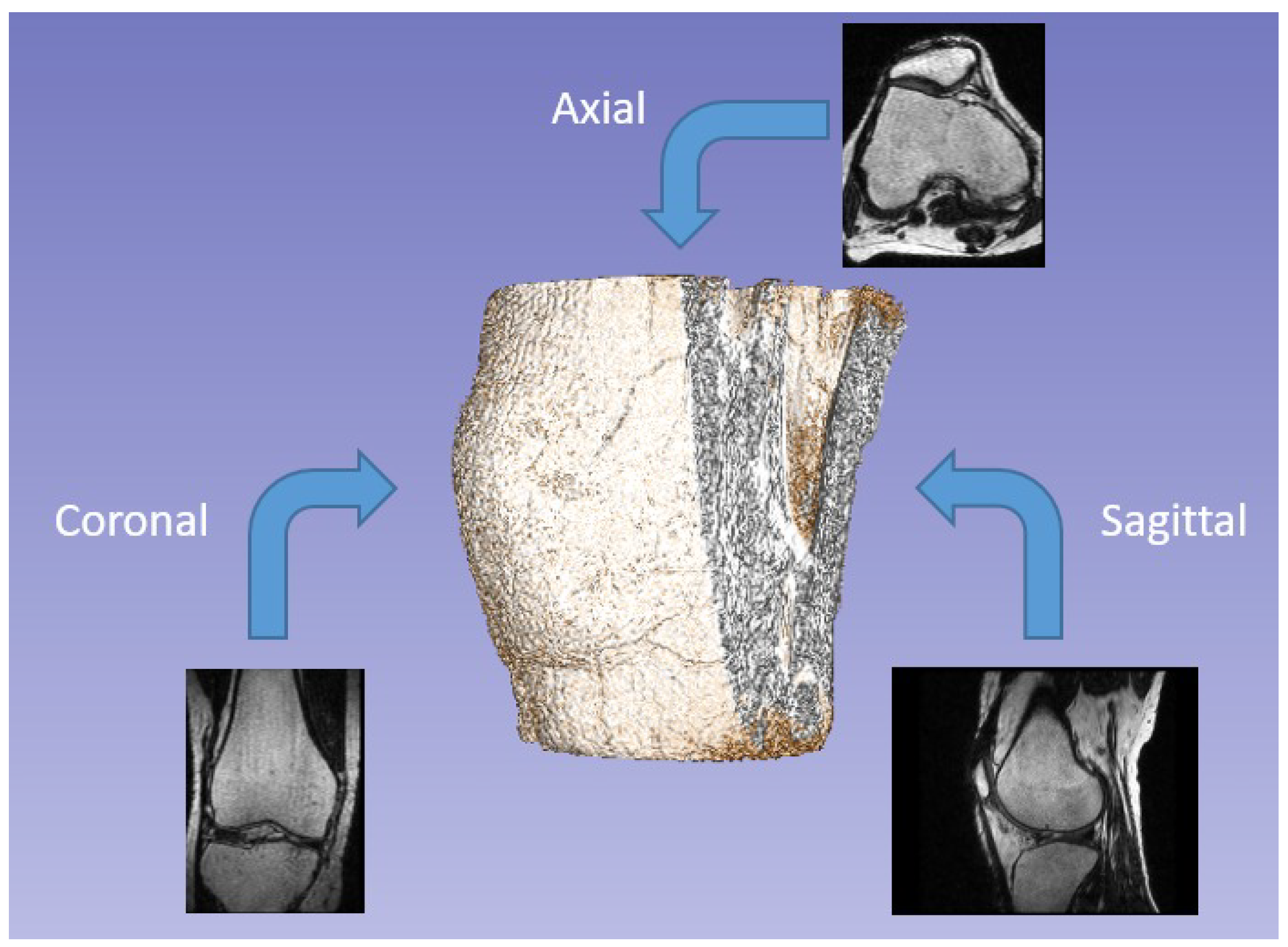
The first approach involved obtaining various projections from the same scan (Figure 1). Since the analyzed data consists of 3D images, the reference unit is the voxel rather than the pixel. Each image’s voxel corresponds to an area of 0.351 mm × 0.351 mm, and the slices are $0.352$ mm apart. This arrangement positions them approximately one pixel apart, resulting in nearly isotropic voxels. The MRI scan used for training is a sagittal view of the knee, but axial and coronal views are also commonly examined during medical assessments. Due to the high-resolution procedure used to generate the scans, there are a total of 286 slices, each with a resolution of $512\times 512$. Consequently, we can perform matrix rotations to create additional projections by treating the entire volume as a three-dimensional array. This process generates new data for training purposes.

Another data augmentation process involved dividing each volume into subsections of size $64\times 64\times 64$, generated with a shift of 32, meaning they overlapped with adjacent subsections (Figure 2). This approach allows the network to process smaller volumes than the original scan, reducing computational load. To ensure precise subdivision, we expanded the initial volume from $286\times 512\times 512$ to $320\times 512\times 512$ by adding empty slices at the end. The axial and coronal projections obtained through the first augmentation process ultimately had a final dimension of $512\times 512\times 320$. This method significantly increased the number of available training samples: 2025 sub-volumes were extracted from each projection, enabling a more detailed study of local morphological features. To perform this volume subdivision, we utilized the Patchify library [17], simplifying the splitting of images into smaller, overlapping patches. Additionally, we developed a custom function to reconstruct the original images from these patches, ensuring proper handling of overlapping adjacent volumes.

We randomly divided the input data into two sets for training the network: $80\%$ for training and $20\%$ for validation. The validation phase, which follows training, is crucial as it assesses the model’s performance on independent data not used during training.

2.3. U-Net

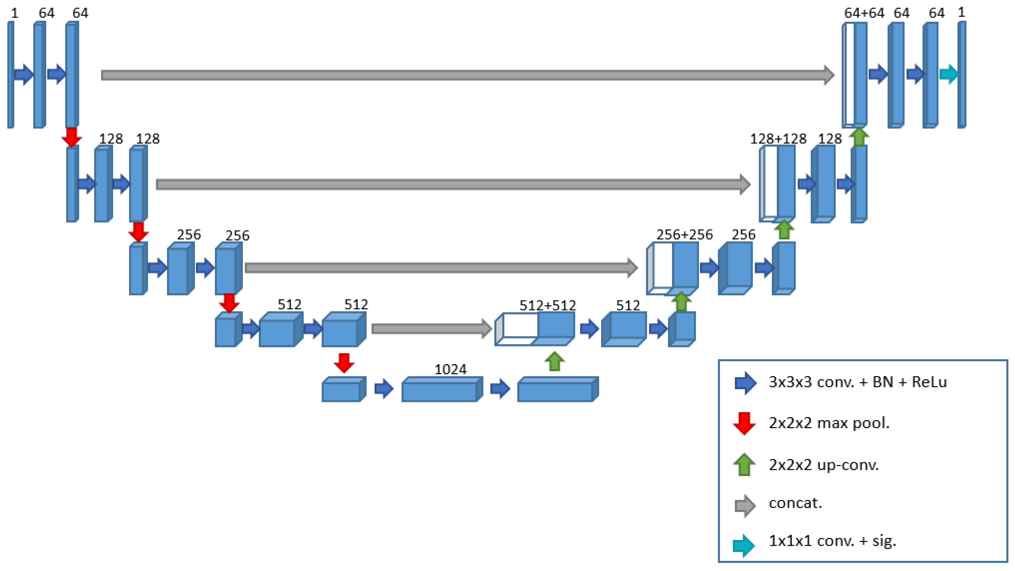
The U-Net [18] is a convolutional neural network initially developed to segment neural biomedical images. In the present study, we employed a 3D network variant, U-Net 3D (Figure 3), specifically designed to segment 3D images such as magnetic resonance imaging or computed tomography (CT) scans. In dealing with volumetric data, a 3D model can be more accurate than a 2D one [19,20]. The 3D approach utilizes correlated information across all spatial dimensions, allowing the model to understand the overall structure of the volume better and maintain coherence between the various slices. In contrast, the 2D approach analyses each slice independently, disregarding the relationships between adjacent slices, which may lead to potential discontinuities in the three-dimensional reconstruction. Furthermore, the 3D approach enhances context capture when recognizing structures that span multiple slices and possess complex geometries, captures spatial and contextual details in three dimensions, and enables precise segmentation of complex anatomical structures.

In addition to extending to the third dimension, the proposed network includes other changes to better adapt to the problem at hand. The network consists of an encoding phase and a decoding phase, the former progressively reduces the spatial dimension of the volume and increases the number of channels, extracting increasingly abstract and high-level features, while the latter performs the opposite operation, reconstructing the segmented image from the extracted features. Each phase comprises specific blocks, which share two operations: two 3D convolutions and the application of the ReLU activation function. Unlike the original paper [18], we chose to perform a batch normalization process after each convolution to normalize the elements and facilitate learning [21,22]. This technique helps stabilize the distribution of inputs, accelerate convergence, and reduce sensitivity to hyperparameters. We will refer to this set of operations as the convolutional block for simplicity. With this premise, we can now describe more clearly the operations performed during the encoding and decoding phases. In the encoding phase, the convolutional block is executed at each step, followed by a 3D max pooling operation with a window size of (2, 2, 2), reducing the volume by half in each dimension and passing the output to the next level. Simultaneously with the reduced volume, the number of feature channels increases for each block. We marked the transition from the encoding phase to the decoding phase with a bridge layer consisting only of a convolutional block with 1024 filters. During the decoding phase, as indicated in the original paper [18], to return to the initial dimension, each block performs an upsampling operation followed by a convolution.

After this process, we merge each output from the final convolution with the output obtained before the max pooling operation from the corresponding encoding block through a concatenation operation. This operation combines the two datasets to generate a single output containing both pieces of information. Without this step, the network would operate solely in a feed-forward manner; however, this concatenation gives the network its distinctive “U” shape. After concatenation, the resulting data are input into a convolutional block as described. In contrast to the encoding phase, in this decoding phase, the number of channels decreases from 512 to 64 as the process progresses. The original work employs the stochastic gradient descent (SGD) algorithm as the optimization method for the learning phase. We opted for the Adam Optimizer [23], which is very popular and widely used in deep neural networks. Adam combines the SGD method with the adaptive moment estimation (AdaGrad) algorithm, and due to its ability to automatically adjust the learning rate and its computational efficiency, it has become one of the preferred optimization algorithms in the deep learning research community. In [23], the authors demonstrated that Adam outperforms other optimizers regarding resource utilization. At the same time, [24] provides a comparison of various optimizers using a CNN for tumor segmentation in brain MRI images, showing that, as in [23], Adam proved to be one of the best choices. Based on this analysis, we chose to use Adam with a learning rate of 0.0001 over SGD.

Additionally, two other changes, closely related to each other compared to the original work, pertain to the activation function for the last layer and the loss function guiding the optimization. Since we are focusing on a binary segmentation problem, we decided to switch from the softmax function to the sigmoid function and from the cross-entropy loss to binary cross-entropy. The sigmoid function is commonly used in image segmentation tasks, particularly for grayscale images, to convert pixel (or voxel) intensity values into a range between 0 and 1. This approach is beneficial because image values can map to a probability of belonging to a class, such as the class of interest. Consequently, we can utilize it to generate a probability map, where higher values indicate a greater likelihood of belonging to the class of interest. This probability map can then be thresholded to produce a binary image that isolates the object of interest. Binary cross-entropy measures the discrepancy between the model’s predictions and the training data. It imposes significant penalties on incorrect predictions, motivating the model to produce probabilities near 1 for positive and 0 for negative examples. Minimizing binary cross-entropy during training effectively maximizes the consistency between the model’s predictions and the training data. This approach helps improve the accuracy and reliability of the segmentation results. These adjustments to the activation function and loss function are crucial for enhancing the performance of the U-Net model in our specific segmentation task, enabling it to produce more accurate and clinically relevant outcomes in the context of knee bone segmentation from MRI scans.

The model was initially trained for 100 epochs with a batch size of 10. A checkpoint callback was implemented to save the model whenever the validation loss reached a new minimum. After each training run, the saved model was analyzed both qualitatively and quantitatively. Although the quantitative results were consistently satisfactory, the focus was primarily on improving the qualitative outcomes. If the qualitative results were unsatisfactory, training was resumed from the previously saved model to refine performance further. This iterative fine-tuning process was repeated several times to optimize the model progressively. Although the number of epochs and optimization settings was not significantly modified between iterations, restarting training from the saved model allowed for continuous improvement and refinement. An important consideration influencing this approach was the limitation of memory resources during training. Due to the large size of the model and the dataset, training for a large number of epochs in a single run could lead to memory overload, which in turn could cause the environment to crash. By saving the model at intermediate stages and continuing training from those checkpoints, it was possible to avoid running out of memory and crashing the environment, thus allowing for a more stable and controlled training process.

2.4. Testing, Post-Processing, and Visualization

We used a similar approach based on volumetric sub-sections during the testing phase, just as we did for learning. As mentioned, we employed a second volumetric scan for testing and decomposed it in the same way as the training data. Consequently, the prediction consists of sub-volumes of the MRI scan. For the testing phase, overlapping the sub-sections during their creation is essential. This feature ensures correct reconstruction of the final volume and prevents gaps between adjacent blocks. Though this condition was unnecessary during the training phase, it was chosen to generate a larger dataset.

Using overlapping 3D patches during inference, predictions are aggregated into the final volume-level segmentation using an overlap-and-add strategy. Each predicted patch is initially in the form of a probability map, where each voxel is assigned a value between 0 and 1 representing the likelihood that the voxel belongs to a region of interest. This is a direct consequence of using a sigmoid activation function in the final layer of the network, which ensures the output values are bounded within the [0, 1] interval. A binary thresholding operation is then applied using a fixed threshold of 0.5 (inclusive), converting these probabilities into a binary mask in which each voxel is labeled as either True (foreground) or False (background). These binary patches are then reassembled into the original volume space by placing them in their respective positions, and overlapping regions are summed voxel-wise. Since the predictions are boolean, this summation implicitly performs a logical OR-like aggregation.

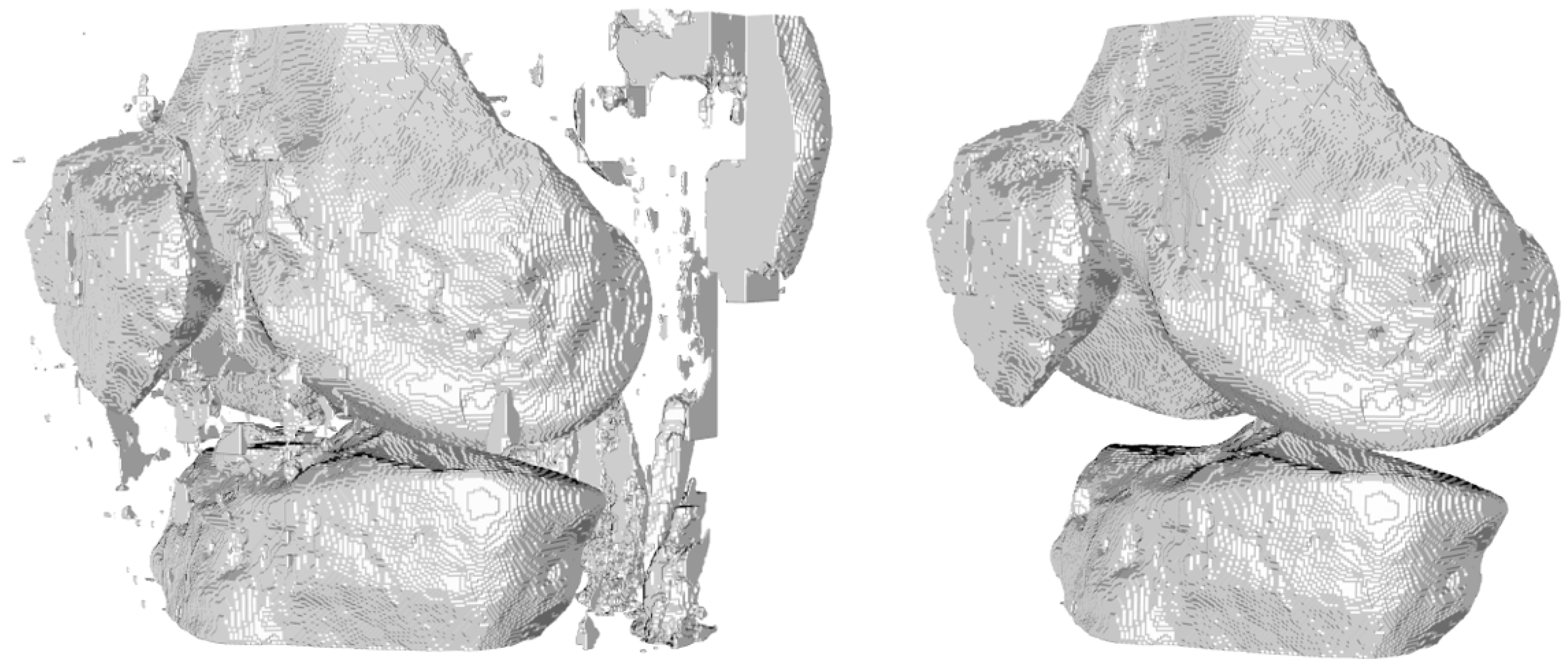
We observed that the dataset’s characteristics—where bones and other anatomical elements exhibited similar intensity within the images—made it challenging for the network to differentiate between different tissues in certain areas. We hypothesized that this difficulty arose because, without a complete view of the image, the network might mistakenly identify bone features in incorrect locations during testing. We implemented a post-processing procedure to address this issue and eliminate any noise from the results. This post-processing assumed that, even though false positive predictions could occur in individual slices, the bones would emerge as the largest volume components in the 3D reconstruction. Therefore, we decided to search the three largest connected 3D components within the results, which should correspond to the tibia, femur, and patella (Figure 4).

The 3D connected components technique, or 3D connected component labeling or 3D region analysis, is a fundamental method in image processing and computer vision used to identify and analyze distinct regions within a three-dimensional image. Unlike the two-dimensional version, which operates on 2D images, the 3D technique identifies and separates contiguous regions within a three-dimensional data volume.

During our analysis of the results, we noticed that the network tends to underestimate positive voxels, leading to false negatives in some regions of the bones. We implemented additional post-processing operations to enhance the accuracy of the obtained volumes. The first of these operations utilizes the network’s capability to segment the knee bones from various projections. This approach takes advantage of information gathered from multiple angles to improve the likelihood of accurately capturing bony structures, thus addressing any segmentation errors caused by incomplete visibility in some sections. From the MRI scan used for testing, which provides an axial view of the knee, we derived the remaining two projections—the sagittal and coronal views—and these three volumes were used individually for testing. Once we obtained the three predictions, they were combined using a voxel-wise logical OR operator to select only the voxels identified in all three projections as correct. It is important to note that to overlap the three volumes, we need their dimensions to match. Therefore, we chose the coronal as the standard projection and converted the axial and sagittal predictions accordingly.

The second post-processing technique is a morphological operation known as closing, which combines two fundamental operations: dilation and erosion (Figure 5). Dilation expands the edges of objects, filling small holes and voids within them, while erosion reduces their size, eliminating noise. The closing operation refines the final segmentation by integrating these two steps: it first expands the edges of the objects to fill small holes, then shrinks those edges back, preserving the filled holes while restoring the objects to their original shape. This process enhances the coherence and continuity of the identified bony structures in the 3D volume.

These post-processing techniques optimize the segmentation results, ensuring a more accurate representation of relevant anatomical structures. In our case, this approach helps to resolve certain inaccuracies without significantly affecting the morphological features of the result, which are the most important characteristics from a medical perspective.

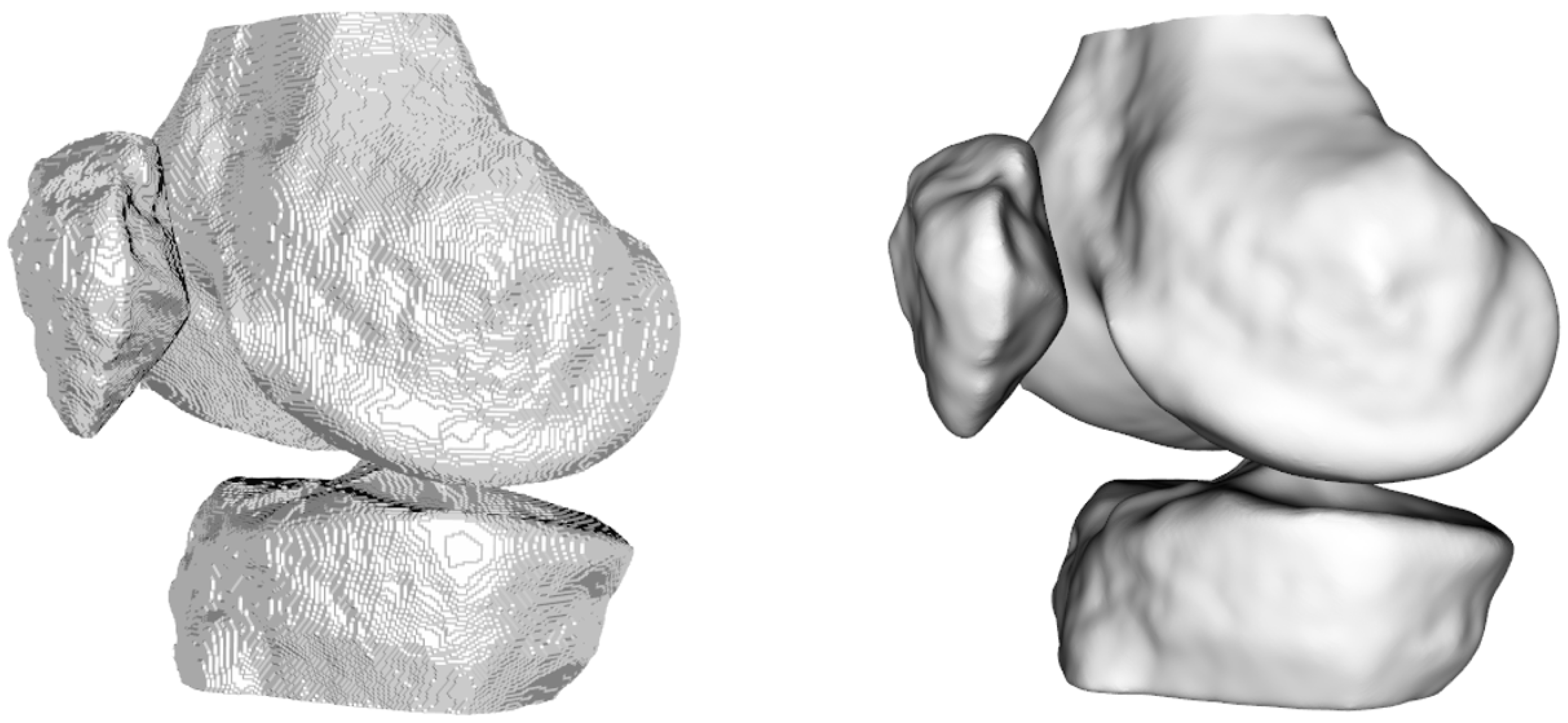
After obtaining the segmentation results, the next step involved visualizing the entire output volume and generating printable 3D surface models (Figure 6). This required converting the voxel-based segmentation into Euclidean coordinates and extracting the isosurfaces corresponding to the femur, tibia, and patella. To improve the quality of the resulting surface meshes, we applied a Laplacian smoothing filter—a mesh-based technique that adjusts vertex positions to reduce local surface irregularities. Specifically, we followed the implementation described in KneeBones3Dify, which we will compare later, where inverse distances between vertices are used as weights [25]. This weighting strategy allows more controlled smoothing, minimizing distortions while preserving the anatomical structure and geometric features of the bones. Unlike simple image-based smoothing filters, this mesh-based method acts directly on the 3D geometry and is well-suited for generating printable surfaces. The smoothed mesh was then exported in STL format, with appropriate voxel-to-millimeter scaling to ensure compatibility with 3D printing software. This approach significantly improves both the visual realism and printability of the 3D models, making them suitable for preoperative visualization and educational purposes.

2.5. Employed Technologies

For the implementation, we used Python (version 3.11.7) with the support of Keras [26] (version 3.3.3) and TensorFlow [27] (version 2.16.1), all executed using Jupyter Notebook [28] (version 7.0.8). To optimize network performance and post-processing, we utilized an NVIDIA RTX A5000 GPU as an accelerator. This GPU targets professional graphics applications, 3D rendering, scientific simulations, and other intensive workloads. By leveraging the CUDA (version 12.6.85) and CuDNN toolkits (version 9.7.0), we significantly improved TensorFlow’s performance.

For the visualization phase, we used the PyCharm (version 2023.3) development environment. It allowed us to visualize the results and apply a C++ function to smooth the final output. We then saved this output as a .stl file, facilitating 3D printing with the appropriate software. It is important to note that we run these codes within the PyCharm environment on a machine equipped with an Intel^® i5-6500 processor that does not have GPU support.

3. Results

In the following section, we will present some quantitative results and compare them with the previously mentioned application, KneeBones3Dify. For this application, we calculated the same metrics used to evaluate the performance of the U-Net 3D on the same scan utilized during our network testing. We computed these metrics after the post-processing step. Additionally, in

Table 1. Model performance evaluation with different radius configurations. The table shows the values of DSC (dice coefficient), IoU (Intersection over Union), AHD (Average Hausdorff Distance), and execution times (CPU only and GPU) for each radius value used.

Closing	DSC	IoU	AHD	Time (CPU)	Time (GPU)
No	0.9752	0.9517	0.0399	4.2441 s	1.4512 s
Radius = 7	0.9829	0.9664	0.0250	266.7015 s	3.3453 s
Radius = 8	0.9832	0.9670	0.0241	319.7278 s	3.7579 s
Radius = 9	0.9838	0.9682	0.0223	455.0744 s	3.9609 s
Radius = 10	0.9840	0.9685	0.0219	603.4697 s	6.1673 s
Radius = 15	0.9844	0.9693	0.0208	2100.4241 s	13.8267 s

, we analyzed the optimal radius for the sphere used as the structuring element in the closing process. We examined how this choice impacted the execution times. We used the best result as a reference for

Table 2. Performance metrics for different bones (femur, tibia, and patella) in the segmentation process.

Bone	DSC	IoU	AHD
Femur	0.9849	0.9703	0.0223
Tibia	0.9848	0.9700	0.0191
Patella	0.9591	0.9401	0.0392

and

Table 3. Comparison of the segmentation performance between the proposed model (3D U-Net) and KneeBones3Dify (KneeBones).

	DSC	IoU	AHD
3D U-Net	0.9838	0.9682	0.0223
KneeBones	0.9015	0.8207	0.4231

. In terms of execution times, the developed application took approximately 227.86 s to predict an entire volume divided into sub-sections.

For this work, several standard metrics were selected from the pymia library [29] to evaluate the performance of the segmentation algorithm. Specifically, the Dice Similarity Coefficient (DSC), Intersection over Union (IoU), and Average Hausdorff Distance (AHD) were used, as they provide complementary insights into the accuracy and quality of the segmentation results. The Dice Similarity Coefficient is a widely used metric to assess the overlap between two segmentations, with higher values indicating better overlap. It has a range of [0, 1], where 1 represents perfect overlap. Intersection over Union similarly quantifies the similarity between two sets, measuring the intersection over the union of the voxel sets. Its range is also [0, 1], with 1 indicating a perfect match between the segmentations. Lastly, the Average Hausdorff Distance (AHD) measures the discrepancy between two segmentations by calculating the average of the Hausdorff distances between them, where lower values are preferable. The range for AHD is [0, +∞], with 0 indicating no spatial dissimilarity. These metrics were chosen for their ability to provide a comprehensive evaluation of both the accuracy of the segmentation overlap and the spatial dissimilarity between the segmented regions, making them ideal for the goals of this study.

From Table 1, it is clear that the results are already excellent from a purely quantitative perspective, even without applying any closing operations. This is because the false negatives, which refer to the missing voxels in the whole volume, represent only a small number of errors compared to the total correctly recognized voxels. Since we are primarily concerned with identifying the bone surface, we are more sensitive to the error in this region than the internal voxels or any potential internal holes, which would not be used for printing. Therefore, we can conclude that while closing operations have a minimal impact on quantitative metrics, they significantly enhance the qualitative aspects of the results.

Continuing the analysis, we observed that as the radius of the structuring element increases, the performance metrics show a noticeable improvement, particularly in the overlap measures such as the DSC and the IoU.

A performance–efficiency trade-off analysis determined the optimal radius for the morphological closing operation. We evaluated multiple radii and compared segmentation metrics (DSC, IoU, and AHD) alongside computational costs (inference time on CPU and GPU), while larger radii led to marginal improvements in segmentation quality, they also significantly increased execution time, particularly on the CPU. Radius 9 was selected as the optimal configuration, as it provided a notable gain in accuracy compared to smaller radii, while maintaining a practical and acceptable execution time. This choice represents the best balance between segmentation quality and computational efficiency for real-world use cases.

When comparing execution times, it is evident that larger radii increase computational cost, whether executed solely on the CPU or also utilizing the GPU, while radius 9 yields a noticeable performance improvement, the execution time remains relatively reasonable: 455.07 s on CPU and 3.96 s on GPU. In contrast, the increase in CPU time becomes much more pronounced for larger radii, with times rising sharply for radius 10 and radius 15, making these configurations less efficient regarding computational resources. Thus, it is crucial to consider the trade-off between performance and computational efficiency, while larger radii (such as 10 and 15) result in further improvements in metrics, the increase in execution time, particularly on the CPU, makes them less ideal for practical use. Therefore, we considered radius 9 the optimal choice, providing the best balance between high segmentation quality and acceptable execution times. Thus, for the analysis presented in Table 2 and Table 3, we used radius 9, as it delivers the best overall performance, offering high-quality segmentation while maintaining reasonable computational costs.

Table 2 presents the application’s performance on individual bones. Analyzing each component can provide valuable insights. The results obtained from the network are excellent, demonstrating high accuracy in segmenting various anatomical structures. Notably, the network effectively segments the patella, one of the most challenging components to isolate due to its proximity to muscles, tendons, and the knee joint capsule.

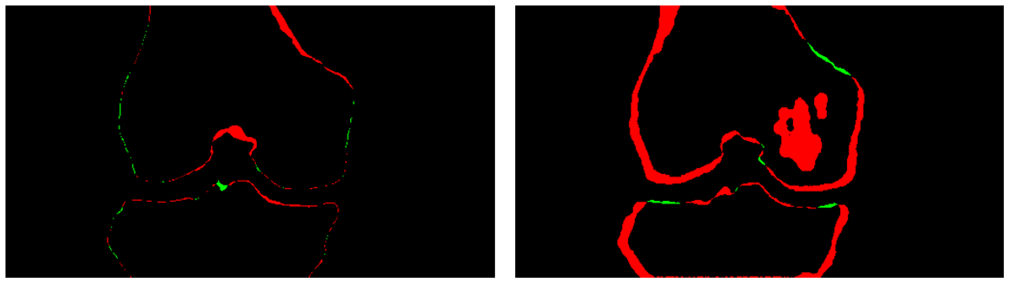
When comparing the metrics with the KneeBones3Dify application (Table 3), we observed that a completely rule-based approach can yield good quantitative results. However, as previously mentioned, it is also crucial to consider the qualitative aspects. Figure 7 illustrates the differences between the results of the two applications and the ground truth. This illustration clearly identifies false positives (in green) and false negatives (in red).

The image on the right, which represents the output of KneeBones3Dify, immediately demonstrates the exceptionally high number of false negatives, particularly along the outer surfaces, while this issue may not be severe from a quantitative perspective—since the metrics still show good values—it raises significant concerns from a qualitative standpoint. The reduction in bone volumes in the results could lead to inaccuracies during potential medical analyses.

4. Discussion

Developing a 3D neural network for volumetric bone segmentation has proven a practical approach, enabling the creation of 3D printable surfaces for clinical assessments. The results demonstrate high accuracy and reliability, closely matching the ground truth. This model was developed through a carefully structured process that included data collection, network design, technical implementation, and performance evaluation, showcasing its potential for accurate and precise segmentation.

However, several challenges remain. A primary concern is the high memory consumption during the training phase, mainly due to the substantial data volumes in 3D images, while optimization techniques such as pruning, quantization, and the adoption of more efficient architectures can enhance overall efficiency, future research should focus on solutions specifically designed to manage and process large data volumes in the context of medical imaging.

We found that subdividing the scans into smaller sub-volumes effectively reduced the computational complexity of the network and increased the available data, all while preserving the ability to analyze individual voxels with their spatial context. However, this approach has limitations; for instance, when splitting the volume into 64 × 64 × 64 sub-sections with a step size of 32, we had to add slices at the end of the volume because the original dimensions were not a multiple of 32, as mentioned in Section 2.

Another area for future exploration involves removing false positives using the 3D connected components method. This method may produce incorrect results when false positives are too close to the bones, potentially merging with the actual bone structures.

Additionally, while the model has shown promising generalization on the test data, its robustness across different imaging protocols, scanners, and patient populations has yet to be thoroughly evaluated. Our study limited itself to MRI scans obtained with specific parameters from low-field, high-resolution scanners. We acknowledge that variations introduced by different scanners or acquisition protocols could influence the model’s performance, which might affect its robustness and generalizability. This is a relevant limitation of the current work, and future studies should focus on testing the model across diverse imaging protocols and datasets, ensuring its applicability in real-world clinical settings, while making precise comparisons with other works is challenging due to the variation in cases and data, it is clear that the implemented model could yield even better results if trained with additional data, providing a strong foundation for future developments.

Our current implementation relied on data augmentation techniques to mitigate overfitting and enhance generalization capabilities. We consider this approach sufficient in the context of our study, as evidenced by the model’s performance on a completely unseen test scan from a different patient. The qualitative and quantitative results—even before post-processing—demonstrated satisfactory performance, suggesting that the model could generalize beyond the training data. Nevertheless, expanding the training dataset with additional scans remains a key direction for improving the model’s robustness and accuracy, especially when aiming for broader clinical deployment.

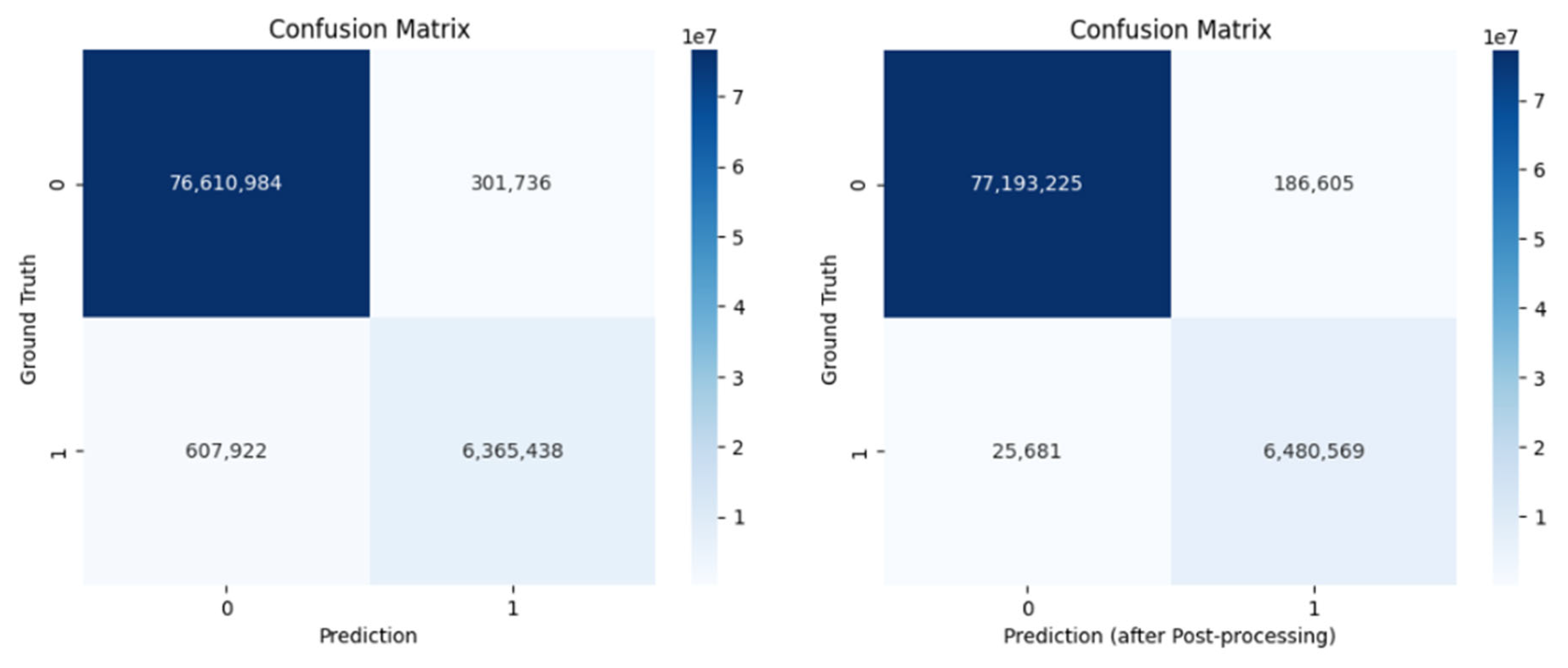
Post-processing proved to be a valuable step in refining the model’s output (Figure 8). In particular, removing false positives was essential to improve the overall quality of the segmentation results, as clearly illustrated in Figure 4, while eliminating false negatives had a more limited impact on the quantitative evaluation metrics (see Table 1), it still enhanced the final visual quality of the predictions. This is especially evident in Figure 7, where the segmentation shows a high degree of overlap with the ground truth, indicating that post-processing helps the model produce cleaner and more precise outputs.

Finally, refining the network architecture and training process could decrease the need for extensive post-processing, improving computational efficiency. Experimentation with alternative architectures, loss functions, or optimization techniques may further improve segmentation accuracy and computational efficiency.

5. Conclusions

This project focused on developing and evaluating a 3D neural network designed for volumetric bone segmentation, with the objective of producing a 3D printable surface for clinical assessments. The analysis reveals that the implemented network achieves remarkable accuracy and reliability, closely aligning with the ground truth.

The project comprised several phases: data collection and preparation, network design, technical implementation, and performance evaluation via various key metrics. Each phase was executed with meticulous attention to detail, ensuring the validity and quality of the results. The findings underscored the model’s ability to segment precisely, demonstrating a significant overlap with the reference data.

This success relies on carefully tuning the network and applying advanced techniques, such as data augmentation and post-processing. Notably, although we trained the network on a single initial sample, its performance on a different test volume yielded excellent results, mainly due to data augmentation. By increasing the volume of input data, the neural network’s ability to generalize improved, allowing it to perform effectively on previously unseen data. Consequently, data augmentation proved essential in enhancing the model’s robustness and versatility, minimizing the risk of overfitting and boosting overall accuracy.

In conclusion, this project successfully demonstrates that three-dimensional neural networks can achieve accurate bone segmentation. The encouraging results lay a solid foundation for future research and development, presenting significant potential for practical applications in automated medical image analysis and precision diagnostics.

References

- Chen, P.; Gao, L.; Shi, X.; Allen, K.; Yang, L. Fully automatic knee osteoarthritis severity grading using deep neural networks with a novel ordinal loss. Comput. Med Imaging Graph. 2019, 75, 84–92. [Google Scholar] [CrossRef] [PubMed]
- Hayashi, D.; Roemer, F.W.; Jarraya, M.; Guermazi, A. Imaging in osteoarthritis. Radiol. Clin. 2017, 55, 1085–1102. [Google Scholar] [CrossRef] [PubMed]
- Lundervold, A.S.; Lundervold, A. An overview of deep learning in medical imaging focusing on MRI. Z. Für Med. Phys. 2019, 29, 102–127. [Google Scholar] [CrossRef]
- Choy, G.; Khalilzadeh, O.; Michalski, M.; Do, S.; Samir, A.E.; Pianykh, O.S.; Geis, J.R.; Pandharipande, P.V.; Brink, J.A.; Dreyer, K.J. Current applications and future impact of machine learning in radiology. Radiology 2018, 288, 318–328. [Google Scholar] [CrossRef] [PubMed]
- Cabitza, F.; Locoro, A.; Banfi, G. Machine learning in orthopedics: A literature review. Front. Bioeng. Biotechnol. 2018, 6, 75. [Google Scholar] [CrossRef]
- Jamshidi, A.; Pelletier, J.P.; Martel-Pelletier, J. Machine-learning-based patient-specific prediction models for knee osteoarthritis. Nat. Rev. Rheumatol. 2019, 15, 49–60. [Google Scholar] [CrossRef]
- Kluzek, S.; Mattei, T. Machine-learning for osteoarthritis research. Osteoarthr. Cartil. 2019, 27, 977–978. [Google Scholar] [CrossRef]
- LeCun, Y.; Bengio, Y.; Hinton, G. Deep learning. Nature 2015, 521, 436–444. [Google Scholar] [CrossRef]
- Geetharamani, G.; Pandian, A. Identification of plant leaf diseases using a nine-layer deep convolutional neural network. Comput. Electr. Eng. 2019, 76, 323–338. [Google Scholar]
- Liu, F.; Zhou, Z.; Jang, H.; Samsonov, A.; Zhao, G.; Kijowski, R. Deep convolutional neural network and 3D deformable approach for tissue segmentation in musculoskeletal magnetic resonance imaging. Magn. Reson. Med. 2018, 79, 2379–2391. [Google Scholar] [CrossRef]
- Ambellan, F.; Tack, A.; Ehlke, M.; Zachow, S. Automated segmentation of knee bone and cartilage combining statistical shape knowledge and convolutional neural networks: Data from the Osteoarthritis Initiative. Med. Image Anal. 2019, 52, 109–118. [Google Scholar] [CrossRef] [PubMed]
- Lim, J.; Kim, J.; Cheon, S. A deep neural network-based method for early detection of osteoarthritis using statistical data. Int. J. Environ. Res. Public Health 2019, 16, 1281. [Google Scholar] [CrossRef]
- Tiulpin, A.; Saarakkala, S. Automatic grading of individual knee osteoarthritis features in plain radiographs using deep convolutional neural networks. Diagnostics 2020, 10, 932. [Google Scholar] [CrossRef]
- Maddalena, L.; Romano, D.; Gregoretti, F.; De Lucia, G.; Antonelli, L.; Soscia, E.; Pontillo, G.; Langella, C.; Fazioli, F.; Giusti, C.; et al. KneeBones3Dify: Open-source software for segmentation and 3D reconstruction of knee bones from MRI data. SoftwareX 2024, 27, 101854. [Google Scholar] [CrossRef]
- Listone, C. clist1/Bone-Segmentation-in-Low-Field-Knee-MRI-Using-a-3D-Convolutional-Neural-Network: 3D U-Net for Low Field Knee MRI. 2025. Available online: https://zenodo.org/records/15372998 (accessed on 10 May 2025). [CrossRef]
- LeCun, Y.; Bottou, L.; Bengio, Y.; Haffner, P. Gradient-based learning applied to document recognition. Proc. IEEE 1998, 86, 2278–2324. [Google Scholar] [CrossRef]
- Wu, W. Patchify, 2017. Available online: https://pypi.org/project/patchify/ (accessed on 23 April 2025).
- Ronneberger, O.; Fischer, P.; Brox, T. U-net: Convolutional networks for biomedical image segmentation. In Proceedings of the Medical Image Computing and Computer-Assisted Intervention–MICCAI 2015: 18th International Conference, Munich, Germany, 5–9 October 2015; proceedings, part III 18. Springer: Berlin/Heidelberg, Germany, 2015; pp. 234–241. [Google Scholar]
- Avesta, A.; Hossain, S.; Lin, M.; Aboian, M.; Krumholz, H.M.; Aneja, S. Comparing 3D, 2.5D, and 2D Approaches to Brain Image Auto-Segmentation. Bioengineering 2023, 10, 181. [Google Scholar] [CrossRef]
- Shivdeo, A.; Lokwani, R.; Kulkarni, V.; Kharat, A.; Pant, A. Comparative Evaluation of 3D and 2D Deep Learning Techniques for Semantic Segmentation in CT Scans. arXiv 2021. [Google Scholar] [CrossRef]
- Ioffe, S.; Szegedy, C. Batch Normalization: Accelerating Deep Network Training by Reducing Internal Covariate Shift. In Proceedings of the 32nd International Conference on Machine Learning, Lille, France, 7–9 July 2015; Proceedings of Machine Learning Research. Bach, F., Blei, D., Eds.; Volume 37, pp. 448–456. [Google Scholar]
- Çiçek, Ö.; Abdulkadir, A.; Lienkamp, S.S.; Brox, T.; Ronneberger, O. 3D U-Net: Learning Dense Volumetric Segmentation from Sparse Annotation. In Proceedings of the Medical Image Computing and Computer-Assisted Intervention—MICCAI 2016, Athens, Greece, 17–21 October 2016; Ourselin, S., Joskowicz, L., Sabuncu, M.R., Unal, G., Wells, W., Eds.; Springer International Publishing: Cham, Switzerland, 2016; pp. 424–432. [Google Scholar]
- Kingma, D.P.; Ba, J. Adam: A method for stochastic optimization. arXiv 2014, arXiv:1412.6980. [Google Scholar]
- Yaqub, M.; Feng, J.; Zia, M.S.; Arshid, K.; Jia, K.; Rehman, Z.U.; Mehmood, A. State-of-the-art CNN optimizer for brain tumor segmentation in magnetic resonance images. Brain Sci. 2020, 10, 427. [Google Scholar] [CrossRef]
- Belyaev, A. Mesh Smoothing and Enhancing. Curvature Estimation. Available online: https://maths.dur.ac.uk/users/norbert.peyerimhoff/epsrc2013/06gm_surf3.pdf (accessed on 23 April 2025).
- Chollet, F. Keras. 2015. Available online: https://keras.io (accessed on 23 April 2025).
- Abadi, M.; Agarwal, A.; Barham, P.; Brevdo, E.; Chen, Z.; Citro, C.; Corrado, G.S.; Davis, A.; Dean, J.; Devin, M.; et al. Tensorflow: Large-scale machine learning on heterogeneous distributed systems. arXiv 2016, arXiv:1603.04467. [Google Scholar]
- Kluyver, T.; Ragan-Kelley, B.; Pérez, F.; Granger, B.; Bussonnier, M.; Frederic, J.; Kelley, K.; Hamrick, J.; Grout, J.; Corlay, S.; et al. Jupyter Notebooks—A publishing format for reproducible computational workflows. In Positioning and Power in Academic Publishing: Players, Agents and Agendas; Loizides, F., Schmidt, B., Eds.; IOS Press: Amsterdam, The Netherlands, 2016; pp. 87–90. [Google Scholar]
- Jungo, A.; Scheidegger, O.; Reyes, M.; Balsiger, F. pymia: A Python package for data handling and evaluation in deep learning-based medical image analysis. Comput. Methods Programs Biomed. 2021, 198, 105796. [Google Scholar] [CrossRef] [PubMed]
- Soscia, E.; Romano, D.; Maddalena, L.; Gregoretti, F.; De Lucia, G.; Antonelli, L. KneeBones3Dify-Annotated-Dataset v1.0.0. 2024. Available online: https://zenodo.org/records/10534328 (accessed on 23 April 2025). [CrossRef]