

A Comparative Study of Ensemble Machine Learning and Explainable AI for Predicting Harmful Algal Blooms


Abstract
1. Introduction
2. Methodology
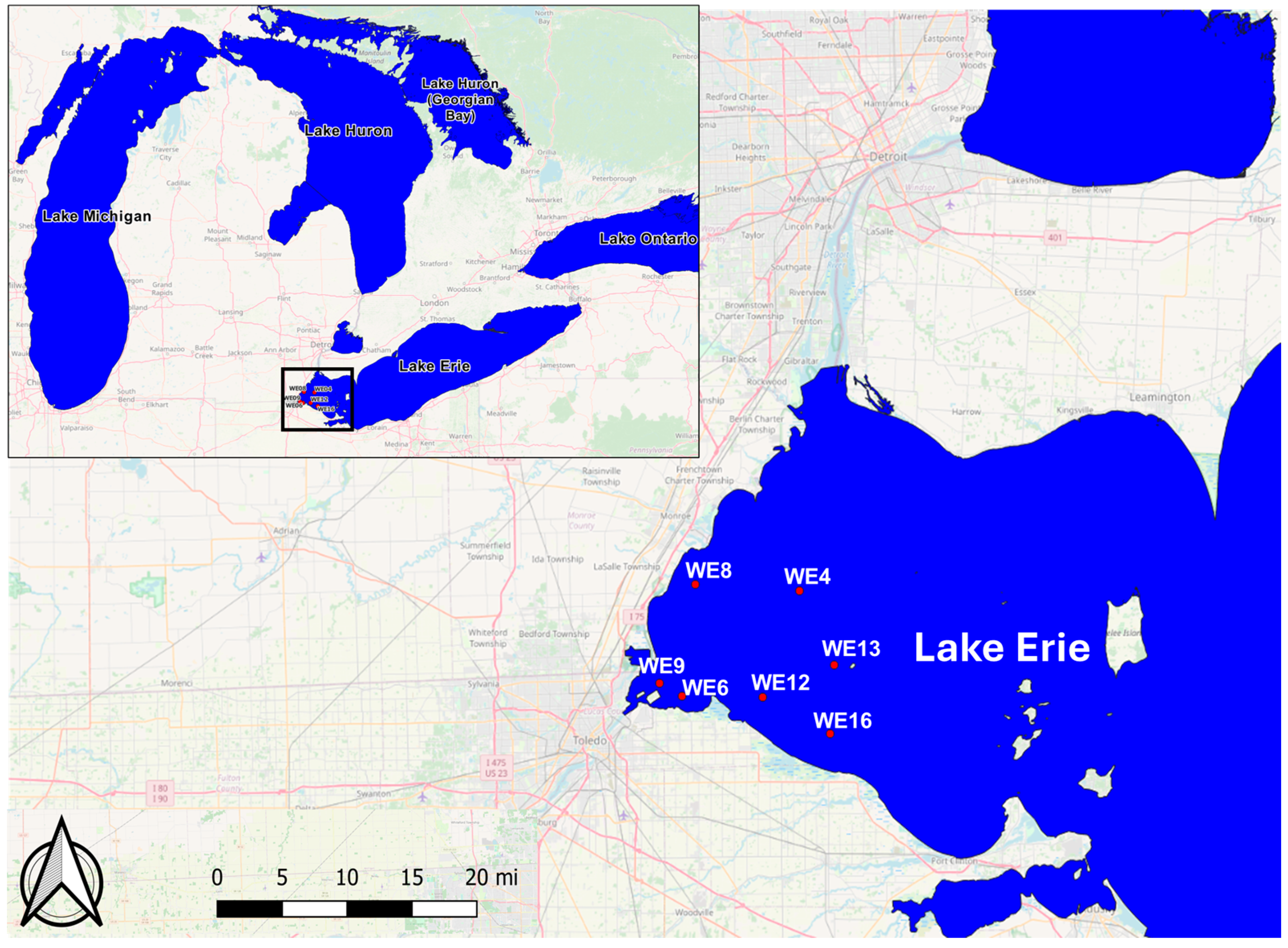
2.1. Study Areas
2.2. Machine Learning Models
2.3. Ensemble Learning Models
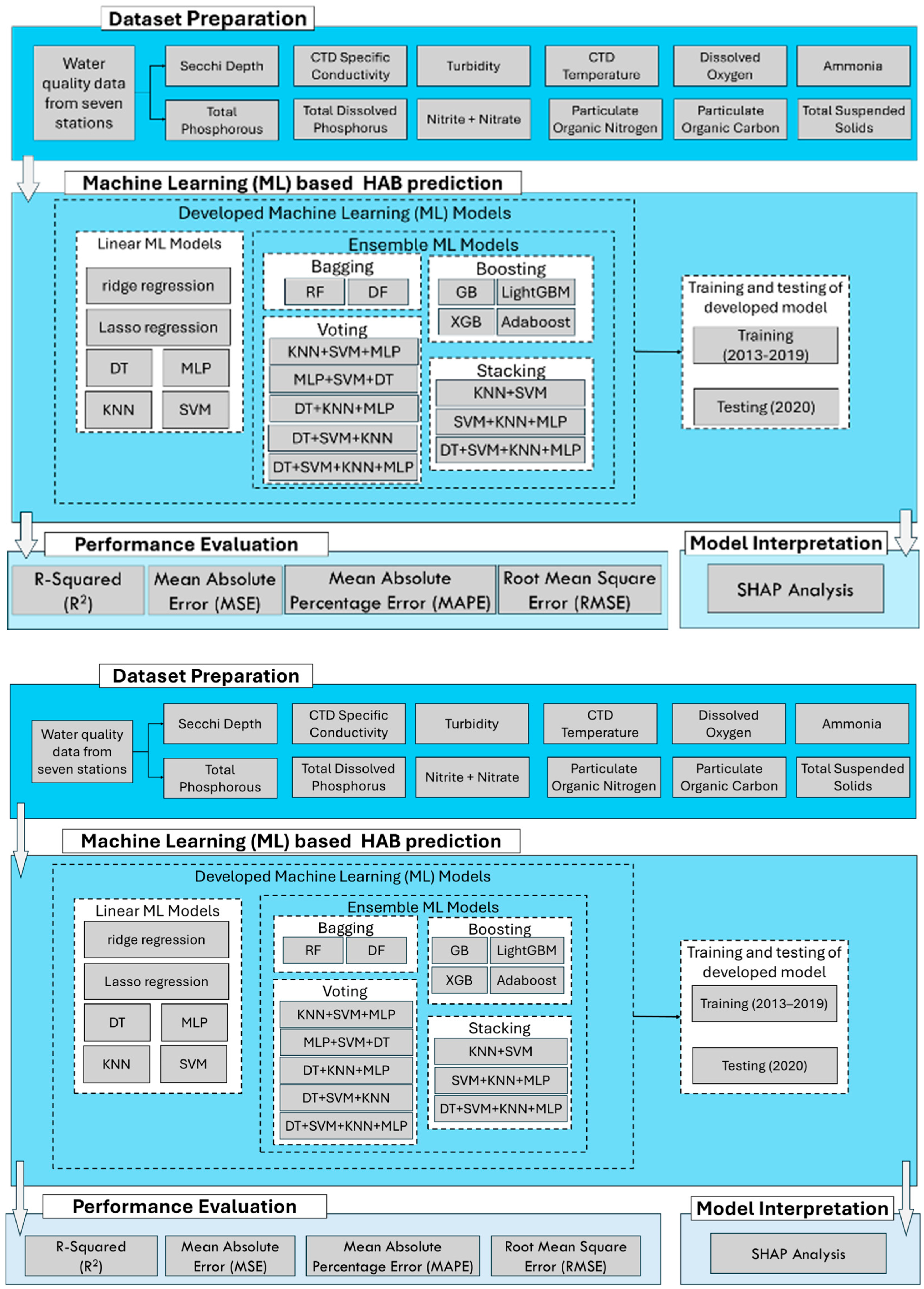
2.4. Model Development
2.5. Model Evaluation
2.6. Model Interpretation Using XAI
3. Results and Discussion
4. Conclusions
Author Contributions
Funding
Data Availability Statement
Acknowledgments
Conflicts of Interest
References
- Carmichael, W.W.; Falconer, I.R. Diseases related to freshwater blue-green algal toxins, and control measures. In Algal Toxins in Seafood and Drinking Water; Falconer, I.R., Ed.; Academic Press: London, UK, 1993; pp. 187–209. [Google Scholar]
- Mount, J.; Sermet, Y.; Jones, C.S.; Schilling, K.E.; Gassman, P.W.; Weber, L.J.; Krajewski, W.F.; Demir, I. An integrated cyberinfrastructure system for water quality resources in the Upper Mississippi River Basin. J. Hydroinformatics 2024, 26, 1970–1988. [Google Scholar] [CrossRef]
- Paerl, H.W.; Paul, V.J. Climate change: Links to global expansion of harmful cyanobacteria. Water Res. 2012, 46, 1349–1363. [Google Scholar] [CrossRef]
- Graham, J.L.; Dubrovsky, N.M.; Eberts, S.M. Cyanobacterial Harmful Algal Blooms and US Geological Survey Science Capabilities. U.S. Geological Survey Report 2016. Available online: https://pubs.usgs.gov/of/2016/1174/ofr20161174_revised.pdf (accessed on 5 December 2024).
- Weirich, C.A.; Miller, T.R. Freshwater harmful algal blooms: Toxins and children’s health. Curr. Probl. Pediatr. Adolesc. Health Care 2014, 44, 2–24. [Google Scholar] [CrossRef]
- Xu, H.; Windsor, M.; Muste, M.; Demir, I. A web-based decision support system for collaborative mitigation of multiple water-related hazards using serious gaming. J. Environ. Manag. 2020, 255, 109887. [Google Scholar] [CrossRef] [PubMed]
- Weber, L.J.; Muste, M.; Bradley, A.A.; Amado, A.A.; Demir, I.; Drake, C.W.; Krajewski, W.F.; Loeser, T.J.; Politano, M.S.; Shea, B.R.; et al. The Iowa Watersheds Project: Iowa’s prototype for engaging communities and professionals in watershed hazard mitigation. Int. J. River Basin Manag. 2017, 16, 315–328. [Google Scholar] [CrossRef]
- Demir, I.; Jiang, F.; Walker, R.V.; Parker, A.K.; Beck, M.B. Information systems and social legitimacy scientific visualization of water quality. In Proceedings of the 2009 IEEE International Conference on Systems, Man and Cybernetics, San Antonio, TX, USA, 11–14 October 2009; pp. 1067–1072. [Google Scholar]
- Sermet, Y.; Demir, I. GeospatialVR: A web-based virtual reality framework for collaborative environmental simulations. Comput. Geosci. 2022, 159, 105010. [Google Scholar] [CrossRef]
- Magnuson, J.J.; Webster, K.E.; Assel, R.A.; Bowser, C.J.; Dillon, P.J.; Eaton, J.G.; Evans, H.E.; Fee, E.J.; Hall, R.I.; Mortsch, L.R. Potential effects of climate changes on aquatic systems: Laurentian Great Lakes and Precambrian Shield Region. Hydrol. Process. 1997, 11, 825–871. [Google Scholar] [CrossRef]
- Tewari, M.; Kishtawal, C.M.; Moriarty, V.W.; Ray, P.; Singh, T.; Zhang, L.; Treinish, L.; Tewari, K. Improved seasonal prediction of harmful algal blooms in Lake Erie using large-scale climate indices. Commun. Earth Environ. 2022, 3, 195. [Google Scholar] [CrossRef]
- Sterner, R.W.; Keeler, B.; Polasky, S.; Poudel, R.; Rhude, K.; Rogers, M. Ecosystem services of Earth’s largest freshwater lakes. Ecosyst. Serv. 2020, 41, 101046. [Google Scholar] [CrossRef]
- Boegehold, A.G.; Burtner, A.M.; Camilleri, A.C.; Carter, G.; DenUyl, P.; Fanslow, D.; Semenyuk, D.F.; Godwin, C.M.; Gossiaux, D.; Johengen, T.H.; et al. Routine monitoring of western Lake Erie to track water quality changes associated with cyanobacterial harmful algal blooms. Earth Syst. Sci. Data 2023, 15, 3853–3868. [Google Scholar] [CrossRef]
- Stumpf, R.P.; Johnson, L.T.; Wynne, T.T.; Baker, D.B. Forecasting annual cyanobacterial bloom biomass to inform management decisions in Lake Erie. J. Great Lakes Res. 2016, 42, 1174–1183. [Google Scholar] [CrossRef]
- Carmichael, W.W.; Boyer, G.L. Health impacts from cyanobacteria harmful algae blooms: Implications for the North American Great Lakes. Harmful Algae 2016, 54, 194–212. [Google Scholar] [CrossRef] [PubMed]
- Buratti, F.M.; Manganelli, M.; Vichi, S.; Stefanelli, M.; Scardala, S.; Testai, E.; Funari, E. Cyanotoxins: Producing organisms, occurrence, toxicity, mechanism of action and human health toxicological risk evaluation. Arch. Toxicol. 2017, 91, 1049–1130. [Google Scholar] [CrossRef]
- Kouakou, C.R.C.; Poder, T.G. Economic impact of harmful algal blooms on human health: A systematic review. J. Water Health 2019, 17, 499–516. [Google Scholar] [CrossRef] [PubMed]
- Yildirim, E.; Demir, I. Agricultural flood vulnerability assessment and risk quantification in Iowa. Sci. Total. Environ. 2022, 826, 154165. [Google Scholar] [CrossRef]
- Islam, S.M.S.; Yeşilköy, S.; Baydaroğlu, Ö.; Yıldırım, E.; Demir, I. State-level multidimensional agricultural drought susceptibility and risk assessment for agriculturally prominent areas. Int. J. River Basin Manag. 2024, 1–18. [Google Scholar] [CrossRef]
- Greene, S.B.D.; LeFevre, G.H.; Markfort, C.D. Improving the spatial and temporal monitoring of cyanotoxins in Iowa lakes using a multiscale and multi-modal monitoring approach. Sci. Total. Environ. 2021, 760, 143327. [Google Scholar] [CrossRef]
- Ratté-Fortin, C.; Plante, J.-F.; Rousseau, A.N.; Chokmani, K. Parametric versus nonparametric machine learning modelling for conditional density estimation of natural events: Application to harmful algal blooms. Ecol. Model. 2023, 482, 110415. [Google Scholar] [CrossRef]
- Paerl, H.W.; Gardner, W.S.; Havens, K.E.; Joyner, A.R.; McCarthy, M.J.; Newell, S.E.; Qin, B.; Scott, J.T. Mitigating cyanobacterial harmful algal blooms in aquatic ecosystems impacted by climate change and anthropogenic nutrients. Harmful Algae 2016, 54, 213–222. [Google Scholar] [CrossRef]
- Yan, Z.; Kamanmalek, S.; Alamdari, N. Predicting coastal harmful algal blooms using integrated data-driven analysis of environmental factors. Sci. Total. Environ. 2023, 912, 169253. [Google Scholar] [CrossRef]
- Demiray, B.Z.; Mermer, O.; Baydaroğlu, Ö.; Demir, I. Predicting harmful algal blooms using explainable deep learning models: A comparative study. Water 2025, 17, 676. [Google Scholar] [CrossRef]
- Boyer, J.N.; Kelble, C.R.; Ortner, P.B.; Rudnick, D.T. Phytoplankton bloom status: Chlorophyll a biomass as an indicator of water quality condition in the southern estuaries of Florida, USA. Ecol. Indic. 2009, 9, S56–S67. [Google Scholar] [CrossRef]
- Mellios, N.K.; Moe, S.J.; Laspidou, C. Using Bayesian hierarchical modelling to capture cyanobacteria dynamics in Northern European lakes. Water Res. 2020, 186, 116356. [Google Scholar] [CrossRef]
- Zhou, Z.-X.; Yu, R.-C.; Zhou, M.-J. Evolution of harmful algal blooms in the East China Sea under eutrophication and warming scenarios. Water Res. 2022, 221, 118807. [Google Scholar] [CrossRef] [PubMed]
- Yeşilköy, S.; Demir, I. Crop yield prediction based on reanalysis and crop phenology data in the agroclimatic zones. Theor. Appl. Clim. 2024, 155, 7035–7048. [Google Scholar] [CrossRef]
- Wells, M.L.; Trainer, V.L.; Smayda, T.J.; Karlson, B.S.; Trick, C.G.; Kudela, R.M.; Ishikawa, A.; Bernard, S.; Wulff, A.; Anderson, D.M.; et al. Harmful algal blooms and climate change: Learning from the past and present to forecast the future. Harmful Algae 2015, 49, 68–93. [Google Scholar] [CrossRef] [PubMed]
- Glibert, P.M. Harmful algae at the complex nexus of eutrophication and climate change. Harmful Algae 2020, 91, 101583. [Google Scholar] [CrossRef]
- Tanir, T.; Yildirim, E.; Ferreira, C.M.; Demir, I. Social vulnerability and climate risk assessment for agricultural communities in the United States. Sci. Total. Environ. 2023, 908, 168346. [Google Scholar] [CrossRef]
- Nourani, V.; Khodkar, K.; Baghanam, A.H.; Kantoush, S.A.; Demir, I. Uncertainty quantification of deep learning-based statistical downscaling of climatic parameters. J. Appl. Meteorol. Clim. 2023, 62, 1223–1242. [Google Scholar] [CrossRef]
- Paerl, H.W.; Hall, N.S.; Calandrino, E.S. Controlling harmful cyanobacterial blooms in a world experiencing anthropogenic and climatic-induced change. Sci. Total. Environ. 2011, 409, 1739–1745. [Google Scholar] [CrossRef]
- Maze, G.; Olascoaga, M.; Brand, L. Historical analysis of environmental conditions during Florida Red Tide. Harmful Algae 2015, 50, 1–7. [Google Scholar] [CrossRef]
- Wells, M.L.; Karlson, B.; Wulff, A.; Kudela, R.; Trick, C.; Asnaghi, V.; Berdalet, E.; Cochlan, W.; Davidson, K.; De Rijcke, M.; et al. Future HAB science: Directions and challenges in a changing climate. Harmful Algae 2020, 91, 101632. [Google Scholar] [CrossRef]
- Katin, A.; Del Giudice, D.; Hall, N.S.; Paerl, H.W.; Obenour, D.R. Simulating algal dynamics within a Bayesian framework to evaluate controls on estuary productivity. Ecol. Model. 2021, 447, 109497. [Google Scholar] [CrossRef]
- Giere, J.; Riley, D.; Nowling, R.J.; McComack, J.; Sander, H. An investigation on machine-learning models for the prediction of cyanobacteria growth. Fundam. Appl. Limnol. 2020, 194, 85–94. [Google Scholar] [CrossRef]
- Greer, B.; McNamee, S.E.; Boots, B.; Cimarelli, L.; Guillebault, D.; Helmi, K.; Marcheggiani, S.; Panaiotov, S.; Breitenbach, U.; Akçaalan, R.; et al. A validated UPLC–MS/MS method for the surveillance of ten aquatic biotoxins in European brackish and freshwater systems. Harmful Algae 2016, 55, 31–40. [Google Scholar] [CrossRef]
- Lombard, F.; Boss, E.; Waite, A.M.; Vogt, M.; Uitz, J.; Stemmann, L.; Sosik, H.M.; Schulz, J.; Romagnan, J.-B.; Picheral, M.; et al. Globally consistent quantitative observations of planktonic ecosystems. Front. Mar. Sci. 2019, 6, 196. [Google Scholar] [CrossRef]
- Rolim, S.B.A.; Veettil, B.K.; Vieiro, A.P.; Kessler, A.B.; Gonzatti, C. Remote sensing for mapping algal blooms in freshwater lakes: A review. Environ. Sci. Pollut. Res. 2023, 30, 19602–19616. [Google Scholar] [CrossRef]
- Kislik, C.; Dronova, I.; Grantham, T.E.; Kelly, M. Mapping algal bloom dynamics in small reservoirs using Sentinel-2 imagery in Google Earth Engine. Ecol. Indic. 2022, 140, 109041. [Google Scholar] [CrossRef]
- Cheng, K.; Chan, S.; Lee, J.H. Remote sensing of coastal algal blooms using unmanned aerial vehicles (UAVs). Mar. Pollut. Bull. 2020, 152, 110889. [Google Scholar] [CrossRef]
- Qiu, Y.; Liu, H.; Liu, F.; Li, D.; Liu, C.; Liu, W.; Huang, J.; Xiao, Q.; Luo, J.; Duan, H. Development of a collaborative framework for quantitative monitoring and accumulation prediction of harmful algal blooms in nearshore areas of lakes. Ecol. Indic. 2023, 156, 111154. [Google Scholar] [CrossRef]
- Bayar, S.; Demir, I.; Engin, G.O. Modeling leaching behavior of solidified wastes using back-propagation neural networks. Ecotoxicol. Environ. Saf. 2007, 72, 843–850. [Google Scholar] [CrossRef] [PubMed]
- Park, J.; Lee, W.H.; Kim, K.T.; Park, C.Y.; Lee, S.; Heo, T.-Y. Interpretation of ensemble learning to predict water quality using explainable artificial intelligence. Sci. Total. Environ. 2022, 832, 155070. [Google Scholar] [CrossRef]
- Wu, N.; Huang, J.; Schmalz, B.; Fohrer, N. Modeling daily chlorophyll a dynamics in a German lowland river using artificial neural networks and multiple linear regression approaches. Limnology 2013, 15, 47–56. [Google Scholar] [CrossRef]
- Huang, J.; Gao, J.; Zhang, Y. Combination of artificial neural network and clustering techniques for predicting phytoplankton biomass of Lake Poyang, China. Limnology 2015, 16, 179–191. [Google Scholar] [CrossRef]
- Liu, M.; Lu, J. Support vector machine―An alternative to artificial neuron network for water quality forecasting in an agricultural nonpoint source polluted river? Environ. Sci. Pollut. Res. 2014, 21, 11036–11053. [Google Scholar] [CrossRef] [PubMed]
- Park, Y.; Cho, K.H.; Park, J.; Cha, S.M.; Kim, J.H. Development of early-warning protocol for predicting chlorophyll-a concentration using machine learning models in freshwater and estuarine reservoirs, Korea. Sci. Total. Environ. 2015, 502, 31–41. [Google Scholar] [CrossRef]
- Derot, J.; Yajima, H.; Jacquet, S. Advances in forecasting harmful algal blooms using machine learning models: A case study with Planktothrix rubescens in Lake Geneva. Harmful Algae 2020, 99, 101906. [Google Scholar] [CrossRef]
- Busari, I.; Sahoo, D.; Harmel, R.D.; Haggard, B.E. Prediction of Chlorophyll-a as an index of harmful algal blooms using machine learning models. J. Nat. Resour. Agric. Ecosyst. 2024, 2, 53–61. [Google Scholar] [CrossRef]
- Jeong, B.; Chapeta, M.R.; Kim, M.; Kim, J.; Shin, J.; Cha, Y. Machine learning-based prediction of harmful algal blooms in water supply reservoirs. Water Qual. Res. J. 2022, 57, 304–318. [Google Scholar] [CrossRef]
- Shin, J.; Yoon, S.; Kim, Y.; Kim, T.; Go, B.; Cha, Y. Effects of class imbalance on resampling and ensemble learning for improved prediction of cyanobacteria blooms. Ecol. Informatics 2021, 61, 101202. [Google Scholar] [CrossRef]
- Ai, H.; Zhang, K.; Sun, J.; Zhang, H. Short-term Lake Erie algal bloom prediction by classification and regression models. Water Res. 2023, 232, 119710. [Google Scholar] [CrossRef]
- Shin, Y.; Kim, T.; Hong, S.; Lee, S.; Lee, E.; Hong, S.; Lee, C.; Kim, T.; Park, M.S.; Park, J.; et al. Prediction of chlorophyll-a concentrations in the Nakdong River using machine learning methods. Water 2020, 12, 1822. [Google Scholar] [CrossRef]
- Clifton, D.S. Classification and regression trees, bagging, and boosting. In Handbook of Statistics; Elsevier: Amsterdam, The Netherlands, 2005; Volume 24, pp. 303–329. [Google Scholar]
- Zhang, D.; Qian, L.; Mao, B.; Huang, C.; Huang, B.; Si, Y. A Data-Driven design for fault detection of wind turbines using random forests and XGboost. IEEE Access 2018, 6, 21020–21031. [Google Scholar] [CrossRef]
- Lin, S.; Liang, Z.; Zhao, S.; Dong, M.; Guo, H.; Zheng, H. A comprehensive evaluation of ensemble machine learning in geotechnical stability analysis and explainability. Int. J. Mech. Mater. Des. 2023, 20, 331–352. [Google Scholar] [CrossRef]
- Saeed, W.; Omlin, C. Explainable AI (XAI): A systematic meta-survey of current challenges and future opportunities. Knowledge-Based Syst. 2023, 263, 110273. [Google Scholar] [CrossRef]
- Arrieta, A.B.; Díaz-Rodríguez, N.; Del Ser, J.; Bennetot, A.; Tabik, S.; Barbado, A.; Garcia, S.; Gil-Lopez, S.; Molina, D.; Benjamins, R.; et al. Explainable Artificial Intelligence (XAI): Concepts, taxonomies, opportunities and challenges toward responsible AI. Inf. Fusion 2020, 58, 82–115. [Google Scholar] [CrossRef]
- Lundberg, S.M.; Lee, S.I. A unified approach to interpreting model predictions. In Advances in Neural Information Processing Systems; The MIT Press: Cambridge, MA, USA, 2017; Volume 30, pp. 4765–4774. [Google Scholar]
- Lundberg, S.M.; Erion, G.; Chen, H.; DeGrave, A.; Prutkin, J.M.; Nair, B.; Katz, R.; Himmelfarb, J.; Bansal, N.; Lee, S.-I. From local explanations to global understanding with explainable AI for trees. Nat. Mach. Intell. 2020, 2, 56–67. [Google Scholar] [CrossRef] [PubMed]
- Cha, Y.; Shin, J.; Go, B.; Lee, D.-S.; Kim, Y.; Kim, T.; Park, Y.-S. An interpretable machine learning method for supporting ecosystem management: Application to species distribution models of freshwater macroinvertebrates. J. Environ. Manag. 2021, 291, 112719. [Google Scholar] [CrossRef]
- Kim, Y.W.; Kim, T.; Shin, J.; Lee, D.S.; Park, Y.S.; Kim, Y.; Cha, Y. Validity evaluation of a machine-learning model for chlorophyll a retrieval using Sentinel-2 from inland and coastal waters. Ecol. Indic. 2022, 137, 108737. [Google Scholar] [CrossRef]
- Baydaroğlu, Ö.; Yeşilköy, S.; Dave, A.; Linderman, M.; Demir, I. Modeling of harmful algal bloom dynamics and integrated web framework for inland waters in Iowa. EarthArxiv 2024. [Google Scholar] [CrossRef]
- Arashi, M.; Roozbeh, M.; Hamzah, N.A.; Gasparini, M. Ridge regression and its applications in genetic studies. PLoS ONE 2021, 16, e0245376. [Google Scholar] [CrossRef]
- Pereira, J.M.; Basto, M.; da Silva, A.F. The logistic lasso and ridge regression in predicting corporate failure. Procedia Econ. Financ. 2016, 39, 634–641. [Google Scholar] [CrossRef]
- Ranstam, J.; Cook, J.A. LASSO regression. J. Brit. Surg. 2018, 105, 1348. [Google Scholar] [CrossRef]
- Sari, A.C. Lasso regression for daily rainfall modeling at Citeko Station, Bogor, Indonesia. Procedia Comput. Sci. 2021, 179, 383–390. [Google Scholar]
- Sammartino, M.; Nardelli, B.B.; Marullo, S.; Santoleri, R. An artificial neural network to infer the mediterranean 3D chlorophyll-a and temperature fields from remote sensing observations. Remote. Sens. 2020, 12, 4123. [Google Scholar] [CrossRef]
- Yu, H.; Kim, S. SVM tutorial—Classification, regression and ranking. In Handbook of Natural Computing, 1st ed.; Rozenberg, G., Bäck, T., Kok, J.N., Eds.; Springer: Berlin/Heidelberg, Germany, 2012; pp. 479–506. [Google Scholar] [CrossRef]
- Wang, Y.; Xie, Z.; Lou, I.; Ung, W.K.; Mok, K.M. Algal bloom prediction by support vector machine and relevance vector machine with genetic algorithm optimization in freshwater reservoirs. Eng. Comput. 2017, 34, 664–679. [Google Scholar] [CrossRef]
- Quinlan, J.R. Induction of decision trees. Mach. Learn. 1986, 1, 81–106. [Google Scholar] [CrossRef]
- Liaw, A.; Wiener, M. Classification and regression by RandomForest. R News 2002, 2, 18–22. Available online: https://journal.r-project.org/articles/RN-2002-022/RN-2002-022.pdf (accessed on 30 April 2025).
- Guo, G.; Wang, H.; Bell, D.; Bi, Y.; Greer, K. KNN Model-Based Approach in Classification. In Proceedings of the OTM Confederated International Conference CoopIS, DOA, and ODBASE, Catania, Italy, 3–7 November 2003; pp. 986–996. [Google Scholar]
- Jung, N.-C.; Popescu, I.; Kelderman, P.; Solomatine, D.P.; Price, R.K. Application of model trees and other machine learning techniques for algal growth prediction in Yongdam reservoir, Republic of Korea. J. Hydroinformatics 2009, 12, 262–274. [Google Scholar] [CrossRef]
- Wang, Y.; Chen, Z.; Shao, H.; Wang, N. A KNN-based classification algorithm for growth stages of Haematococcus pluvialis. In Proceedings of the 2021 IEEE 4th Advanced Information Management, Communicates, Electronic and Automation Control Conference (IMCEC), Chongqing, China, 18–20 June 2021; Volume 4. [Google Scholar]
- Breiman, L. Random forests. Mach. Learn. 2001, 45, 5–32. [Google Scholar] [CrossRef]
- Zhou, Z.H.; Feng, J. Deep forest. Natl. Sci. Rev. 2019, 6, 74–86. [Google Scholar] [CrossRef] [PubMed]
- Friedman, J.H. Greedy function approximation: A gradient boosting machine. Ann. Stat. 2001, 29, 1189–1232. [Google Scholar] [CrossRef]
- Chen, T.; Guestrin, C. XGBoost: A scalable tree boosting system. In Proceedings of the 22nd ACM SIGKDD International Conference on Knowledge Discovery Data Mining, San Francisco, CA, USA, 13–17 August 2016; pp. 785–794. [Google Scholar]
- Prabha, A.; Yadav, J.; Rani, A.; Singh, V. Design of intelligent diabetes mellitus detection system using hybrid feature selection based XGBoost classifier. Comput. Biol. Med. 2021, 136, 104664. [Google Scholar] [CrossRef]
- Ghatkar, J.G.; Singh, R.K.; Shanmugam, P. Classification of algal bloom species from remote sensing data using an extreme gradient boosted decision tree model. Int. J. Remote. Sens. 2019, 40, 9412–9438. [Google Scholar] [CrossRef]
- Ke, G.; Meng, Q.; Finley, T.; Wang, T.; Chen, W.; Ma, W.; Ye, Q.; Liu, T.-Y. LightGBM: A highly efficient gradient boosting decision tree. In Proceedings of the Advances in Neural Information Processing Systems, Long Beach, CA, USA, 4–9 December 2017; Volume 30, pp. 3146–3154. [Google Scholar]
- Hatwell, J.; Gaber, M.M.; Azad, R.M.A. Ada-WHIPS: Explaining AdaBoost classification with applications in the health sciences. BMC Med. Informatics Decis. Mak. 2020, 20, 250. [Google Scholar] [CrossRef]
- Bauer, E.; Kohavi, R. An empirical comparison of voting classification algorithms: Bagging, boosting, and variants. Mach. Learn. 1999, 36, 105–139. [Google Scholar] [CrossRef]
- Wolpert, D.H. Stacked generalization. Neural Netw. 1992, 5, 241–259. [Google Scholar] [CrossRef]
- Ly, Q.V.; Tong, N.A.; Lee, B.-M.; Nguyen, M.H.; Trung, H.T.; Le Nguyen, P.; Hoang, T.-H.T.; Hwang, Y.; Hur, J. Improving algal bloom detection using spectroscopic analysis and machine learning: A case study in a large artificial reservoir, South Korea. Sci. Total Environ. 2023, 901, 166467. [Google Scholar] [CrossRef]
- Demiray, B.Z.; Sit, M.; Mermer, O.; Demir, I. Enhancing hydrological modeling with transformers: A case study for 24-h streamflow prediction. Water Sci. Technol. 2024, 89, 2326–2341. [Google Scholar] [CrossRef]
- Jiang, J.; Zhou, H.; Zhang, T.; Yao, C.; Du, D.; Zhao, L.; Cai, W.; Che, L.; Cao, Z.; Wu, X.E. Machine learning to predict dynamic changes of pathogenic Vibrio spp. abundance on microplastics in marine environment. Environ. Pollut. 2022, 305, 119257. [Google Scholar] [CrossRef]
- Stubblefield, J.; Hervert, M.; Causey, J.L.; Qualls, J.A.; Dong, W.; Cai, L.; Fowler, J.; Bellis, E.; Walker, K.; Moore, J.H.; et al. Transfer learning with chest X-rays for ER patient classification. Sci. Rep. 2020, 10, 20900. [Google Scholar] [CrossRef]
- Burkart, N.; Huber, M.F. A survey on the explainability of supervised machine learning. J. Artif. Intell. Res. 2021, 70, 245–317. [Google Scholar] [CrossRef]
- Wang, G.; Zhou, W.; Cao, W.; Yin, J.; Yang, Y.; Sun, Z.; Zhang, Y.; Zhao, J. Variation of particulate organic carbon and its relationship with bio-optical properties during a phytoplankton bloom in the Pearl River estuary. Mar. Pollut. Bull. 2011, 62, 1939–1947. [Google Scholar] [CrossRef] [PubMed]
- Zhou, Z.-X.; Yu, R.-C.; Zhou, M.-J. Resolving the complex relationship between harmful algal blooms and environmental factors in the coastal waters adjacent to the Changjiang River estuary. Harmful Algae 2017, 62, 60–72. [Google Scholar] [CrossRef] [PubMed]
- Du, Y.; An, S.; He, H.; Wen, S.; Xing, P.; Duan, H. Production and transformation of organic matter driven by algal blooms in a shallow lake: Role of sediments. Water Res. 2022, 219, 118560. [Google Scholar] [CrossRef]
- Zhang, X.; Li, Y.; Zhao, J.; Wang, Y.; Liu, H.; Liu, Q. Temporal dynamics of the Chlorophyll a-Total phosphorus relationship and algal production efficiency: Drivers and management implications. Ecol. Indic. 2024, 158, 111339. [Google Scholar] [CrossRef]
- Zhai, S.; Yang, L.; Hu, W. Observations of atmospheric nitrogen and phosphorus deposition during the period of algal bloom formation in Northern Lake Taihu, China. Environ. Manag. 2009, 44, 542–551. [Google Scholar] [CrossRef]
- Dai, G.; Shang, J.; Qiu, B. Ammonia may play an important role in the succession of cyanobacterial blooms and the distribution of common algal species in shallow freshwater lakes. Glob. Change Biol. 2012, 18, 1571–1581. [Google Scholar] [CrossRef]
- Wurtsbaugh, W.A.; Paerl, H.W.; Dodds, W.K. Nutrients, eutrophication and harmful algal blooms along the freshwater to marine continuum. WIREs Water 2019, 6, e1373. [Google Scholar] [CrossRef]

| Variables | WE4 | WE6 | WE8 | WE9 | WE12 | WE13 | WE16 | |
|---|---|---|---|---|---|---|---|---|
| Independent variables | SD | 1.96 (0.95) | 0.69 (0.51) | 1.14 (0.85) | 0.36 (0.18) | 0.88 (0.65) | 1.57 (0.93) | 1.38 (1.02) |
| T | 21.73 (3.61) | 21.85 (4.31) | 21.98 (4.14) | 22.73 (4.07) | 21.89 (3.77) | 21.96 (3.47) | 22.77 (3.14) | |
| Cond | 245.49 (23.54) | 350.34 (59.38) | 298.18 (50.51) | 388.2 (69.46) | 282.91 (47.43) | 249.57 (26.55) | 275.6 (32.19) | |
| DO | 7.69 (1.07) | 7.6 (1.24) | 7.72 (1.21) | 7.09 (1.3) | 7.61 (1.02) | 7.74 (1.01) | 7.21 (0.95) | |
| Turb | 5.59 (6.8) | 32.06 (72.07) | 21.64 (94.48) | 40.37 (49.34) | 17.5 (21.68) | 9.75 (19.08) | 8.73 (7.08) | |
| TP | 24.26 (16.2) | 127.03 (146.9) | 83.24 (225.15) | 168.9 (123.17) | 65.91 (55.52) | 32.27 (29.07) | 36.24 (21.28) | |
| TDP | 5.93 (5.36) | 35.03 (38.11) | 18.36 (25.69) | 45.91 (34.4) | 18.89 (23.1) | 7.48 (9.04) | 11.88 (15.62) | |
| A | 25.71 (49.08) | 35.79 (50.74) | 29.6 (41.98) | 72.56 (84.5) | 36.47 (183.73) | 18.12 (32.78) | 18.64 (21.21) | |
| N | 0.37 (0.3) | 1.52 (1.85) | 0.83 (1) | 1.85 (2.05) | 0.73 (1.16) | 0.34 (0.37) | 0.44 (0.56) | |
| POC | 1.08 (1.13) | 4.53 (17.85) | 3.66 (16.63) | 3.24 (3.84) | 1.62 (1.36) | 1.3 (1.49) | 1.18 (0.7) | |
| PON | 0.18 (0.19) | 0.74 (2.83) | 0.65 (3.34) | 0.56 (0.67) | 0.27 (0.23) | 0.22 (0.24) | 0.2 (0.12) | |
| TSS | 6.18 (6.01) | 29.02 (50.1) | 15.78 (36.6) | 37.93 (41.6) | 17.17 (20.51) | 10.03 (16.97) | 8.95 (6.2) | |
| Dependent variable | Chl-a | 15.22 (20.16) | 50.4 (63.9) | 37.49 (70.9) | 47.09 (65.35) | 22.53 (26.84) | 17.11 (22.29) | 15.5 (11.12) |
| Models | Parameters |
|---|---|
| Ridge Regression | Alpha = 100 |
| Lasso Regression | Alpha = 100 |
| KNN | N_neighbors = 30 |
| DT | Min_samples_split = 2; min_samples_leaf = 1 |
| MLP | Epochs = 2000; learning rate = 0.001; batch size = 32 |
| SVM | Kernel = rbf; c = 100,000 |
| LightGBM | Leaves: 31; learning_rate: 0.05; rounds: 100; feature_fraction: 0.9 |
| RF | N_estimators = 1000 |
| AdaBoost | N_estimators = 100; learning_rate = 0.1 |
| DF | N_estimators = 50 |
| GB | N_estimators = 1000 |
| XGBoost | Num_rounds = 100; learning_rate = 0.05 |
| Model | R2 | MAE | MAPE | RMSE |
|---|---|---|---|---|
| Ridge Regression | 0.419 | 11.609 | 1.364 | 13.948 |
| Lasso Regression | 0.423 | 11.590 | 1.367 | 13.907 |
| KNN | 0.604 | 8.848 | 0.907 | 11.513 |
| DT | 0.719 | 6.169 | 0.469 | 9.703 |
| MLP | 0.766 | 6.340 | 0.406 | 8.606 |
| SVM | 0.816 | 5.108 | 0.428 | 7.851 |
| Ensemble Models | Performance Metrics | ||||
|---|---|---|---|---|---|
| R2 | MAE | MAPE | RMSE | ||
| Bagging | RF | 0.848 | 4.776 | 0.414 | 7.312 |
| DR | 0.854 | 4.537 | 0.403 | 6.983 | |
| Boosting | GB | 0.724 | 7.297 | 0.597 | 9.617 |
| XGB | 0.852 | 4.919 | 0.427 | 7.047 | |
| LightGBM | 0.783 | 5.227 | 0.467 | 8.525 | |
| Adaboost | 0.787 | 6.839 | 0.954 | 8.442 | |
| Stacking | S#1 (KNN + SVM) | 0.799 | 5.397 | 0.471 | 8.203 |
| S#2 (SVM + KNN + MLP) | 0.811 | 5.234 | 0.469 | 7.951 | |
| S#3 (DT + SVM + MLP + KNN) | 0.823 | 5.043 | 0.447 | 7.696 | |
| Voting | V#1 (MLP + SVM +KNN) | 0.769 | 6.558 | 0.691 | 8.798 |
| V#2 (MLP + SVM + DT) | 0.836 | 5.066 | 0.529 | 7.413 | |
| V#3 (MLP + KNN + DT) | 0.763 | 6.512 | 0.725 | 8.919 | |
| V#4 (SVM + KNN + DT) | 0.845 | 4.921 | 0.483 | 7.202 | |
| V#5 (MLP + SVM + KNN + DT) | 0.645 | 8.764 | 1.148 | 10.907 | |
| Model | Training Runtime |
|---|---|
| Lasso | 1.0 s |
| Ridge | 1.0 s |
| MLP | 144.9 s |
| RF | 5.2 s |
| LightGBM | 7.0 s |
| SVM | 12.7 s |
| Adaboost | 5.2 s |
| DT | 1.0 s |
| KNN | 0.5 s |
| DF | 561.8 s |
| GB | 1.0 s |
| XGBoost | 1.0 s |
| ML Models | Input Features (Mean |SHAP|) | ||||
|---|---|---|---|---|---|
| Lasso | TP (25) | Turb (6.5) | A (2.0) | TDP (1.5) | POC (0.5) |
| Ridge | TP (35) | Turb (10) | A (2.5) | TDP (2.0) | POC (0.7) |
| KNN | N (6.0) | TDP (3.5) | DO (2.5) | Temp (2.0) | Cond (1.1) |
| DT | PON (20.0) | POC (6.0) | A (4.0) | Turb (2.5) | DO (2.0) |
| MLP | TP (15.0) | Turb (12.2) | A (10.0) | POC (5.3) | PON (2.0) |
| AdaBoost | PON (14.5) | POC (2.2) | A (1.8) | Temp (0.3) | N (0.1) |
| LightGBM | PON (17.7) | POC (7.5) | A (2.8) | Turb (2.7) | TP (2.5) |
| RF | PON (9.5) | POC (6.0) | A (2.5) | Turb (1.8) | Temp (1.5) |
| SVM | PON (24) | POC (12) | TP (7.5) | TDP (6.0) | N (5.9) |
| GB | PON (25) | POC (6) | TP (5) | Turb (5) | A (4.5) |
| XGBoost | PON (18) | POC (7) | A (3) | Turb (2.7) | Temp (2.5) |
| DF | PON (14) | POC (5) | A (2) | Turb (1.5) | N (1) |
Disclaimer/Publisher’s Note: The statements, opinions and data contained in all publications are solely those of the individual author(s) and contributor(s) and not of MDPI and/or the editor(s). MDPI and/or the editor(s) disclaim responsibility for any injury to people or property resulting from any ideas, methods, instructions or products referred to in the content. |
© 2025 by the authors. Licensee MDPI, Basel, Switzerland. This article is an open access article distributed under the terms and conditions of the Creative Commons Attribution (CC BY) license (https://creativecommons.org/licenses/by/4.0/).
Share and Cite
Mermer, O.; Zhang, E.; Demir, I. A Comparative Study of Ensemble Machine Learning and Explainable AI for Predicting Harmful Algal Blooms. Big Data Cogn. Comput. 2025, 9, 138. https://doi.org/10.3390/bdcc9050138
Mermer O, Zhang E, Demir I. A Comparative Study of Ensemble Machine Learning and Explainable AI for Predicting Harmful Algal Blooms. Big Data and Cognitive Computing. 2025; 9(5):138. https://doi.org/10.3390/bdcc9050138
Chicago/Turabian StyleMermer, Omer, Eddie Zhang, and Ibrahim Demir. 2025. "A Comparative Study of Ensemble Machine Learning and Explainable AI for Predicting Harmful Algal Blooms" Big Data and Cognitive Computing 9, no. 5: 138. https://doi.org/10.3390/bdcc9050138
APA StyleMermer, O., Zhang, E., & Demir, I. (2025). A Comparative Study of Ensemble Machine Learning and Explainable AI for Predicting Harmful Algal Blooms. Big Data and Cognitive Computing, 9(5), 138. https://doi.org/10.3390/bdcc9050138