Article

Machine Learning-Based Classification of Sulfide Mineral Spectral Emission in High Temperature Processes

by
Carlos Toro
1,*,
Walter Díaz
2,
Gonzalo Reyes
2,
Miguel Peña
2,
Nicolás Caselli
1,
Carla Taramasco
3,
Pablo Ormeño-Arriagada
4 and
Eduardo Balladares
2
1
Faculty of Engineering, Universidad Andres Bello, Autopista Concepción-Talcahuano CCP-THNO 7100, Talcahuano 4260000, Chile
2
Metallurgical Engineering Department, University of Concepción, Concepción 4070386, Chile
3
Department of Engineering Sciences, Universidad Andres Bello, Viña del Mar 2531015, Chile
4
Facultad de Ingeniería, Negocios y Ciencias Agroambientales, Universidad de Viña del Mar, Viña del Mar 2520000, Chile
*
Author to whom correspondence should be addressed.
Big Data Cogn. Comput. 2025, 9(5), 130; https://doi.org/10.3390/bdcc9050130
Submission received: 14 April 2025 / Revised: 7 May 2025 / Accepted: 13 May 2025 / Published: 14 May 2025
(This article belongs to the Special Issue Machine Learning and AI Technology for Sustainable Development)

Abstract

Accurate classification of sulfide minerals during combustion is essential for optimizing pyrometallurgical processes such as flash smelting, where efficient combustion impacts resource utilization, energy efficiency, and emission control. This study presents a deep learning-based approach for classifying visible and near-infrared (VIS-NIR) emission spectra from the combustion of high-grade sulfide minerals. A one-dimensional convolutional neural network (1D-CNN) was developed and trained on experimentally acquired spectral data, achieving a balanced accuracy score of 99.0% in a test set. The optimized deep learning model outperformed conventional machine learning methods, highlighting the effectiveness of deep learning for spectral analysis in high-temperature environments. In addition, Gradient-weighted Class Activation Mapping (Grad-CAM) was applied to enhance model interpretability and identify key spectral regions contributing to classification decisions. The results demonstrated that the model successfully distinguished spectral features associated with different mineral species, offering insights into combustion dynamics. These findings support the potential integration of deep learning for real-time spectral monitoring in industrial flash smelting operations, thereby enabling more precise process control and decision-making.

1. Introduction

Pyrometallurgy has been one of the principal methods used for copper extraction, it involves the application of high temperature to refine copper concentrates by separating valuable metals from unwanted materials. These processes typically require a large amount of energy and can produce gas and particle emissions [1].
Among these processes, flash smelting is one of the main methods for melting copper and nickel concentrates worldwide. This technology was introduced in the late 1940s and involves feeding previously dried mineral concentrates into a high temperature reaction shaft along with oxygen-enriched air enabling rapid smelting in a controlled environment. This can result in high grade metal compounds recovery and reduced gas and particle emissions [2,3]. Since this technology was implemented, two main lines of research have been followed: the first focused on a better understanding of the combustion phenomena that occur in the furnace’s reaction tower at a laboratory scale [4,5,6,7,8,9,10,11], and the second focused on the continuous improvement of the operation, highlighting the evaluation of the performance of concentrators and burners [12,13].
At the industrial level, tests have been conducted for the development of phenomenological and dynamic models to understand the operation of flash furnaces in real-time [14,15,16]. Despite advances, achieving combustion optimization and characterization supported by sensing technologies remains a significant scientific and technical challenge, primarily because of the extreme operational conditions present in industrial flash furnaces. To address this challenge, researchers have increasingly turned to optical and radiometric techniques to gain insights into combustion phenomena, as these methods offer advantages such as contactless, non-invasive measurements and resistance to electromagnetic interference. For instance, several studies have employed radiometric techniques in laboratory experiments to analyze mineral combustion and estimate the ignition temperature of particles [17,18,19,20], as well as to measure combustion cloud temperature in industrial flash furnaces [20,21].
Recently, in laboratory settings, it has been possible to automatically recognize the VIS-NIR emission spectra of sulfides composing copper concentrates, with a focus on pyrite and chalcopyrite minerals, using multivariate analytical methods [21], as well as unmixing the spectral patterns of iron and copper oxides [22]. In this work, and following these efforts, we apply and test different machine learning and deep learning modeling methodologies to classify one-dimensional spectral signals produced by the emitted VIS-NIR radiation from the combustion of different sulfide minerals. In this context, the key contributions of this article include:
  • Collection of a VIS-NIR emission spectral dataset of high-grade sulfide minerals during combustion. The dataset comprises 8294 spectral signals in the spectral range from 400 to 900 nm with a total of 2576 intensity samples, and it includes spectra from eight mineral species: bornite, chalcocine, chalcopiryte, coveline, enargite, magnetite, pyrite and pyrrhotite.
  • Development of machine and deep learning models for the classification of emission spectral data. We implement and compare multiple classification approaches, including traditional machine learning and deep learning architectures such as 1D-CNNs. Emphasis is placed on model selection, hyperparameter tuning, and validation procedures to ensure generalization.
  • Application of an adapted explainability method to enhance model interpretability. To address the black-box nature of deep learning models, we incorporate Grad-CAM as a post-hoc interpretability method. We generate heatmaps over the spectral input space, allowing us to visualize which spectral regions of the spectrum contributed most to the model’s classification decisions, and to correlate these identified features with known chemical emission lines and oxidation patterns of the sulfide minerals.
The remainder of this paper is structured as follows: Section 2 presents background and related work, focusing on previous studies in spectroscopy, and the application of machine and deep learning techniques in spectral data analysis. Section 3 details the methodology, including the experimental setup designed for the high-temperature combustion of sulfide minerals, the procedures for acquiring visible and near-infrared emission spectra, and the data processing steps. In Section 4, we report and discuss the modeling results obtained from various classification algorithms, including traditional machine learning and 1D convolutional neural networks, along with the integration of explainability techniques. Finally, Section 5 summarizes the conclusions drawn from the study, provides practical implications for industrial applications, and suggests directions for future research in this area.

2. Background and Related Work

Spectroscopy is an analytical technique used to study the interaction between electromagnetic radiation and matter. Depending on the spectral region and the type of interaction analyzed, spectroscopy methods can be broadly categorized into emission, absorption and reflection modalities. Emission spectroscopy measures the radiation emitted by excited atoms or molecules, while absorption spectroscopy quantifies the energy absorbed by substances. Reflection spectroscopy evaluates the reflection characteristics of materials upon interaction with photons from an external radiation source. In this work, emission spectra produced by the combustion of minerals is measured with a spectrometer that can collect and digitalize these signals in the VIS-NIR spectral region (about 400 nm to 900 nm). Figure 1 illustrates the primary modalities of spectroscopic and radiometric measurement methods, with a focus on a mineral particle and typical instrumentation that can be used, highlighting the type of collected digital data.
To extract meaningful information from these different data modalities, scientists from machine learning and analytical chemistry fields have proposed and adapted analytical methods depending on the application needs. Advances in machine learning (ML) and deep learning (DL) methodologies have significantly improved this analysis, offering automated, efficient, and accurate classification and quantification compared to traditional chemometric methods [23,24,25].
Recent studies report on the potential of ML and DL algorithms to analyze spectral signals for mineral identification and chemical composition estimation. Jahoda et al. [23] demonstrated that deep learning, particularly convolutional neural networks (CNNs), significantly surpasses classical methods for mineral classification based on a fusion of Raman and VIS-NIR spectral signals, improving the classification accuracy. Es-sahly et al. [24] applied ML algorithms such as partial least squares-discriminant analysis (PLS-DA), random forests, and support vector machines (SVMs) to short-wave infrared (SWIR) spectroscopy, achieving accurate separation of copper minerals from waste rock with up to 90% classification accuracy. Smith et al. developed interpretable ML models capable of classifying uranium minerals based on Raman spectra, linking spectral features to understand vibrational modes and providing chemically meaningful explanations for model predictions [26]. Further emphasizing applications in metallurgical processes, Bernicky et al. [27] designed an artificial neural network (ANN) combined with flame emission spectroscopy to accurately determine the elemental composition (Cu, Fe, S, Si, Zn) of powdered minerals relevant to copper smelting. Their ANN model achieved excellent predictive accuracy without sample preparation, demonstrating robustness in both laboratory mixtures and industrial samples, significantly outperforming traditional chemometric methods.
Moreover, since spectral measurements in different modalities are one-dimensional (1D) signals, as shown in Figure 1, 1D-CNN are commonly implemented. These architectures follow a structure analogous to CNNs used for two-dimensional (2D) images, incorporating distinct stages for feature extraction and classification (or regression), but constraining the input, convolutional filter dimensions, and pooling operations exclusively to one dimension. For instance, in [25], the authors introduced a framework that integrated portable NIR spectroscopy with 1D-CNN models, transfer learning, and sensor fusion to accurately predict soil properties, such as pH, organic and inorganic content, and nutrients in field conditions. Yang et al. [28] used micro-Fourier Transform Infrared (FTIR) spectroscopy with a 1D-CNN model to detect early-stage citrus Huanglongbing disease by monitoring callose accumulation in phloem tissue, outperforming conventional chemometric methods. Additionally, Li et al. [29] used NIR spectroscopy and 1D-CNNs for jujube variety classification, achieving peak accuracies of up to 94.25% even with limited data. Sang et al. [30] developed a deep 1D-CNN model for mineral classification using Raman spectra, achieving a high performance in accurately recognizing hundreds of mineral species, even with unbalanced datasets. Qi et al. [31] employed Raman spectroscopy and deep learning techniques for the rapid identification of 2D materials. They developed a four-layer 1D-CNN architecture, enhanced by data augmentation using Denoising Diffusion Probabilistic Models, to classify Raman spectra of various 2D materials. This approach achieved a classification accuracy of 98.8% on the original dataset, which improved to 100% with the augmented data, demonstrating the efficacy of deep learning-assisted Raman spectroscopy for automated and high-precision materials analysis. These developments highlight the synergy between ML and DL in spectroscopic analysis, enabling accurate materials and objects identification.
Despite their effectiveness, deep learning models are often criticized as “black boxes” due to their complex internal workings, posing a barrier to their industrial acceptance [32]. For instance, in spectral analysis, it is particularly important to identify the spectral regions that contribute the most to certain prediction results because this can provide insights into the underlying physical, biological, or chemical properties of the measured samples [32,33]. To address this issue, explainability techniques such as Grad-CAM [34,35,36] have appeared as an alternative for model transparency, and it is implemented in this work for the deep learning modeling approach. This method allows visualization of important spectral regions by generating heatmaps that highlight the most influential features in the classification process. It computes the gradients of the predicted class score with respect to the last convolutional layer, and as a result, generates a weighted activation map that emphasizes the most relevant spectral features. For instance, in materials science, Wang et al. [37] integrated FTIR with a 1D-CNN and Grad-CAM to precisely measure the thickness of multilayer composite plastic films, significantly reducing prediction errors. Thus, our proposed framework not only fills a gap in sulfide mineral spectral classification using modern AI methods but also aligns with broader trends in the digital transformation of high-temperature industrial operations. By combining deep learning, explainability, and high-resolution spectral data, this research contributes to the advancement of intelligent monitoring and process optimization tools in pyrometallurgy.

3. Materials and Methods

This study was conducted using an experimental combustion setup at the “Igor Wilkomirsky” Metallurgical Laboratory at the University of Concepción, Chile. The experimental framework was designed to simulate controlled high-temperature oxidation conditions of the sulfide minerals.

3.1. Experimental Setup and Spectral Acquisition

For each experimental run, the goal was to obtain the emission spectra for each mineral sulfide, in this work, bornite, chalcocine, chalcopiryte, coveline, enargite, magnetite, pyrite and pyrrhotite were combusted. The setup consisted of a “Drop-Tube” furnace heated with electrical resistances coated in thermal insulating material, allowing us to reach a maximum temperature of 1200 °C [22]. To perform spectral measurements, the furnace was heated to 1000 °C.
A custom-designed lance with a water-cooling system was introduced into the furnace at the top. Through this lance, oxygen and nitrogen were injected into the furnace in a ratio of 8:2, respectively, and the gas flow rate was controlled by flowmeters and adjusted to ensure laminar flow conditions inside the drop-tube. The sulfide particles were introduced into the furnace at a rate of 5 g/min using a rotatory feeder positioned at the top of the lance.
Driven by the high temperature and presence of oxygen, the particles in their fall are heated and combusted. During these reactions the radiation emitted by the particles was captured by a cooled optical fiber (Avantes®), this optical fiber is introduced through the lance. The optical fiber then guides the radiation to a VIS-NIR spectrometer (Ocean Optics USB4000®), which has spectral sensitivity and a higher signal-to-noise ratio (SNR) in the spectral range from 400 nm to 900 nm with an average spectral resolution of ~0.22 nm, delivering a total of 2576 intensity samples. The spectrometer was calibrated to measure the emitted radiation I in absolute irradiance units (µW/(cm2 ∙ nm)) according to procedures depicted in [20,22]. To transform the I r a w spectral signal in digital counts to absolute irradiance, we can apply the following calibration equation:
I ( λ , T )   = H c a l ( λ ) I r a w ( λ , T ) I d ( λ ) t i A D ( λ )
where λ is the wavelength, T is the combustion temperature, H c a l ( λ ) is the spectral response of a calibration lamp, in this work, the HL-2000-CAL lamp manufactured by Ocean Optics was used, t i is the integration time in seconds, A is the collection area from the optical fiber in cm2 and D(λ) is the wavelength spread of the sensor [24]. Thus, the collected emission spectra from the combustion reactions can be modeled as I ( λ , T ) = I c ( λ , T ) + I d ( λ , T ) + I m o l ( λ , T ) + e + d , with I c a continuous baseline described by Planck’s radiation law, I m o l and I d are spectral signals associated with molecular and elemental (discrete) emissions, and e and d are the electronic and dark current noise components, respectively. Dark current noise is corrected during the calibration step as seen in (1).
The spectrometer’s integration time was adjusted to maximize the SNR while avoiding signal saturation. This parameter had to be evaluated individually for each experimental run, as different minerals emitted varying levels of radiative intensity during combustion. Once combusted, all particles exiting the bottom of the furnace were captured in a water container to stop reactions and for later analysis, whereas the gases were drawn into the washing system for neutralization. The experimental setup is shown in Figure 2.

3.2. Spectral Signal Processing

The spectral data analysis consisted of an exploratory analysis and modeling stage. In the first step, the calibrated spectra were arranged in a data matrix, and Principal Component Analysis (PCA) was applied for exploratory analysis to the raw and standardized spectral data.
Before the classification modeling step, the spectral data from each mineral species were randomly shuffled and then split into two sets: a training set (80%) and a testing set (20%), ensuring that the spectra from each mineral species were represented proportionally. Finally, the training subsets were combined into a single data matrix. The same procedure was applied to the test subsets. Classification algorithms were then implemented and trained in Python® (version 3.11.12) using Scikit-learn (version 1.6.1) and Keras libraries (version 3.8.0).
Prior to applying PCA and any classification algorithm, each spectrum was standardized using z-score normalization. This preprocessing step transforms each spectral sample from a spectrum I ( λ i ) in the data matrix into a standardized form I * ( λ i ) with zero mean and unit variance, according to I * ( λ i ) = ( I ( λ i ) μ i ) / σ i , where μ i and σ i denote the mean and standard deviation at the i-th spectral variable, respectively. To prevent data leakage and ensure proper generalization, μ i and σ i were computed solely from the training set. These parameters were then applied to transform the corresponding test set. This preprocessing, implemented using the StandardScaler function from the Scikit-learn library, ensures that all spectral bands contribute equally to the analysis and enhances numerical stability during model optimization.
In this work, the following machine learning algorithms were implemented: (i) Nearest Neighbors (KNN), (ii) Support Vector Machines (SVM), (iii) Decision Tree (DT), (iv) Histogram Boosting (HB) and (v) Random Forest (RF). And for the deep learning approach, a fully connected artificial neural network (ANN) and 1D-CNN architecture were designed.
All machine learning models were trained using a standard free-tier Google Colab environment, which includes a dual-core CPU and approximately 12 GB of RAM. In contrast, the deep learning models were trained using a GPU-accelerated runtime (NVIDIA A100 with 40 GB memory) also available via Google Colab Pro tier, enabling faster training and hyperparameter tuning iterations due to improved computational throughput.

3.3. Machine and Deep Learning Modeling Strategies

To ensure robust and unbiased model selection and performance estimation for the machine learning approach, we implemented a nested cross-validation (CV) strategy using Scikit-learn. This approach is particularly suitable when hyperparameter tuning is involved, as it avoids information leakage from the test data into the model selection process.
The nested cross-validation procedure consisted of an outer loop for model evaluation and an inner loop for hyperparameter optimization. The outer loop was implemented using stratified K-fold cross validation [38] with 5 splits, ensuring that each fold preserves the original class distribution. For the inner loop, we applied randomized search and cross validation with 3 splits to efficiently explore the hyperparameter space of each algorithm, optimizing for the balance accuracy (BAcc) score—a metric particularly suited for imbalanced classification problems. This score is calculated as the average of recall (Table 1) obtained on each class, meaning it gives equal weight to the accuracy of each class, regardless of how many samples belong to each. In other words, it is defined as:
BAcc   = 1 K i = 1 K T P i T P i + F N i
where
K = Number of classes
T P i = True Positives for class i, i.e., correctly classified instances of class i,
F N i = False Negatives for class i, i.e., Instances of class i wrongly classified as another class.
Table 1. Definitions and formulas of the metrics used to evaluate performance of optimized models.
MetricDefinitionFormula
Accuracy
(Acc)
Proportion of correctly predicted instances among all predictions Accuracy = i = 1 K T P i Total   number   of   predictions
PrecisionProportion of correctly predicted instances among all predicted positives ( F P i is the number of false positives for class i) Precision i = T P i T P i   +   F P i
Recall Proportion of correctly predicted instances among all actual positives Recall i = T P i T P i   +   F N i
F1-scoreHarmonic mean of Precision and Recall F 1 - score i = 2 × Precision i Recall i Precision i   +   Recall i
For a deep comparison of model performance in the test set, we additionally computed the traditional accuracy score for all predictions and a precision, recall, and F1-score for each class. These metrics provide complementary insights and were computed using Scikit-learn’s classification_report function and averaged using both macro and weighted schemes to account for class imbalance. Table 1 summarizes the definitions and formulas of the metrics used in the model evaluation.
For each model, a relevant hyperparameter space was defined in Scikit-learn based on preliminary experiments conducted on the training dataset. The selected hyperparameters were chosen to control the complexity, learning behavior, and decision boundaries of each algorithm, ensuring flexibility to adapt to the spectral characteristics of the combustion data. Table 2 depicts the selected hyperparameters space for each algorithm, including their explored value ranges.
Then, deep learning model architectures based on fully connected ANN and a 1D-CNN were evaluated. Hyperparameters for these architectures were optimized using a Hyperband Search method [39] implemented in the Keras Tuner library (version 1.4.7 in this work). The Hyperband hyperparameter optimization algorithm employs principled early stopping to allocate resources efficiently. Unlike Bayesian optimization, which relies on surrogate modeling and sequential updates, hyperband explores a broad range of configurations and quickly discards underperformers. This approach enhances scalability in high-dimensional spaces and can achieve up to a 30× speedup over Bayesian methods [38], making it particularly effective in resource-constrained environments.
Hyperparameters such as: (i) number of hidden layers (1 to 5) and their corresponding number of neurons (128 to 2576 with steps of 128) in the fully connected architecture, (ii) activation functions in both models (rectified linear unit or hyperbolic tangent) and (iii) number of filters (from 16 to 256 with steps of 16), kernel size (odd numbers between 3 and 25 included), and number of convolutional layers in the 1D-CNN architecture were optimized.
In addition, note that for similar problems involving spectra measured in different modalities, a good performance is achieved with a few hidden or convolutional layers, as reported by other authors [40], in which a maximum of four is defined for these hyperparameters during their optimization. Here, we defined the search space from 1 to 5 convolutional layers and one fully connected layer for the classification stage.
Adaptive Moment Estimation (Adam) [41] was implemented with chosen starting learning rates of 10−2, 10−3 or 10−4 during hyperparameter optimization. Also, it is important to note that during the hyperparameters search and configuration of the Hyperband method, the number of epochs was intentionally limited to 15 to reduce computational cost and accelerate the search process, given that the training procedure was time-consuming.
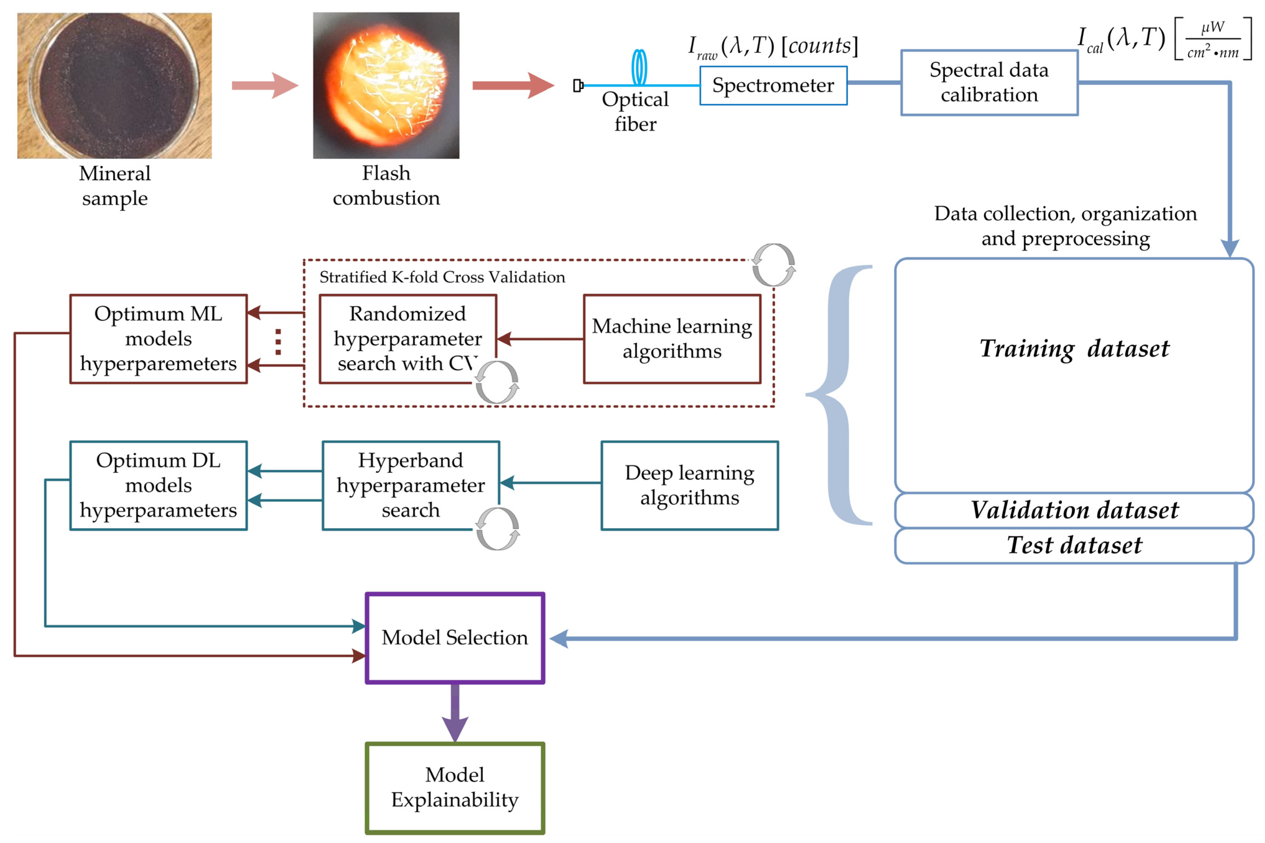
In all cases, a sparse categorical cross-entropy loss function was implemented, and the output layers used a SoftMax activation function because the mineral species in question are mutually exclusive, and this activation function is well suited for such data. The full dataset was divided into a proportion of 8:1:1 for training, validation, and testing in these experiments. Finally, the complete acquisition and modeling workflow is summarized and illustrated schematically in Figure 3.
After the hyperparameter optimization process, both final architectures were trained with a batch size of 64 samples and a limit of 300 epochs. An early stopping strategy with a patience of 20 epochs, which evaluate improvements on validation accuracy, was implemented to avoid overfitting and improve models’ generalization.

4. Results and Discussion

4.1. Mineral Spectral Emission Data

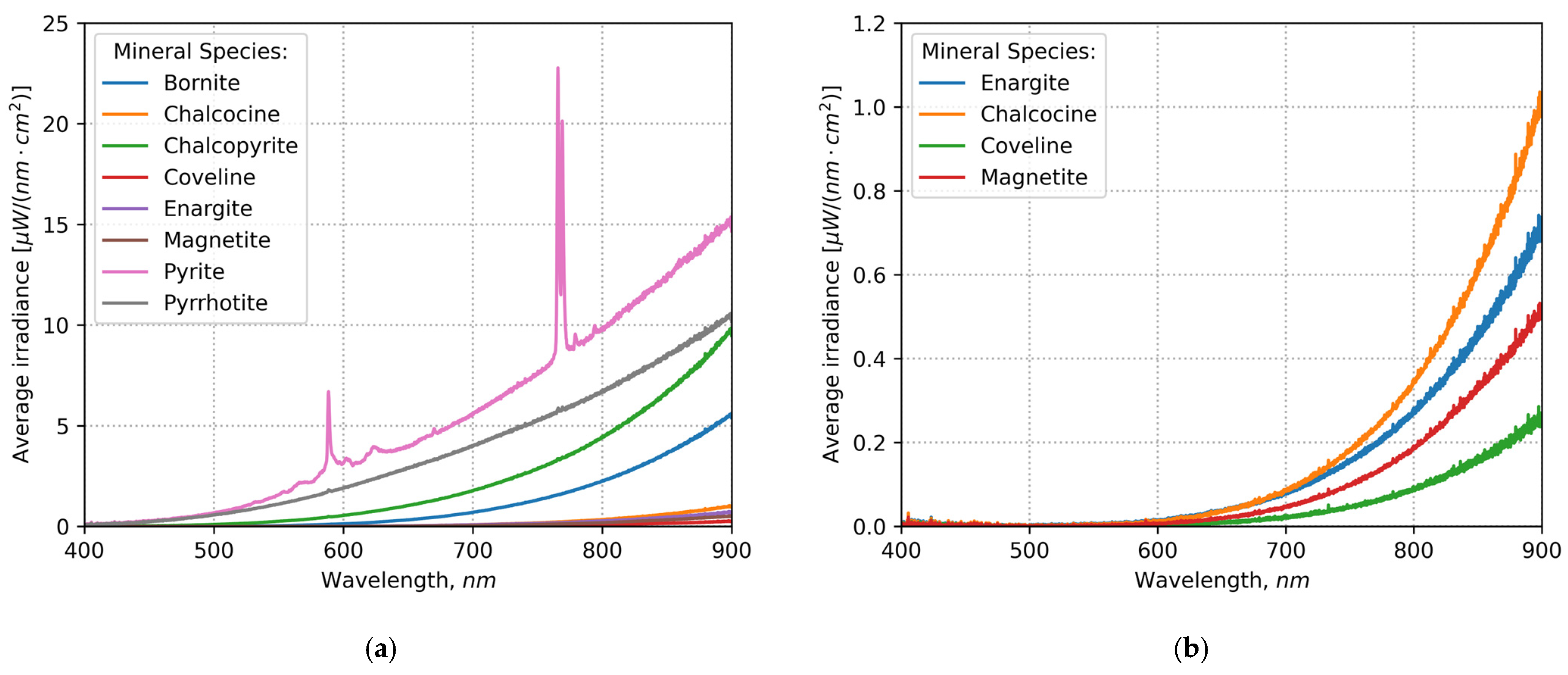
In Figure 4, the average emitted spectra captured from the combustion of each mineral species are shown. Figure 4a shows that pyrite presents the highest intensities at almost all wavelengths, possibly because its oxidation reaction is the most exothermic among the sulfides studied. In this spectrum, spike signals, commonly known as spectral peaks, at 588 nm and two more at 765–769 nm are seen, also appear in pyrrhotite emission but with lower amplitudes. These peaks are associated with sodium and potassium emissions [20,21,22]. The emission spectra of species such as chalcocine, coveline, enargite, and magnetite showed lower intensities that did not exceed the average value of 1 µW/(cm2 ∙ nm), as shown in Figure 4b. Physically, the minerals in Figure 4b decompose at temperatures close to 1000 °C; thus, the degree of oxidation of these sulfides remains low for a short period, leading to low-intensity emission spectra. In addition, the oxidation of magnetite is an endothermic reaction that absorbs energy from the system and causes a decrease in the temperature, resulting in a low-intensity spectrum.
The total collected spectral signals for each mineral were as follows: (i) 104 for bornite, (ii) 281 for chalcocine, (iii) 3127 for chalcopyrite, (iv) 370 for coveline, (v) 174 for enargite, (vi) 253 for magnetite, (vii) 961 for pyrite and (viii) 3024 for pyrrhotite. Although the dataset was unbalanced, owing to the unavailability of some minerals and complex spectral acquisition for low emissive species, generalization was not affected during the modeling and evaluation stages. The dataset was also published online and can be accessed here [42]. The folder contains all the analyzed spectral signals and is saved in the Numpy file format—.npy.
To the best of our knowledge, no publicly available datasets report emission spectra from mineral samples under high-temperature conditions comparable to those described in this work. While existing datasets focus primarily on reflectance-mode VIS-NIR spectroscopy [43], the dataset presented here is, to our understanding, the first to provide calibrated flame emission data for mineral classification tasks. This reinforces its value for benchmarking and future reproducibility efforts in similar research domains.

4.2. Principal Component Analysis

Figure 5 illustrates the score plots for the first two principal components and their distributions obtained from PCA applied to both the raw and preprocessed data. In the case of the raw data (Figure 5a), the first two principal components capture 99.24% of the total variance. In contrast, after preprocessing (Figure 5b), these two principal components account for approximately 96.5% of the spectral data variance. This difference may be attributed to the standardization step, which reduces variability caused by differences in intensity or scale across spectral measurements. Although this preprocessing slightly decreases the variance explained by the first two components, it enhances the interpretability of the PCA model by mitigating the impact of scale differences among the measured spectra. These figures also highlight subtle distinctions among the analyzed mineralogical species, particularly pyrite, pyrrhotite, and chalcopyrite. Although some species scores overlapped, the observed patterns suggest exploring and testing nonlinear classification algorithms such as deep learning approaches, to enhance classification performance.
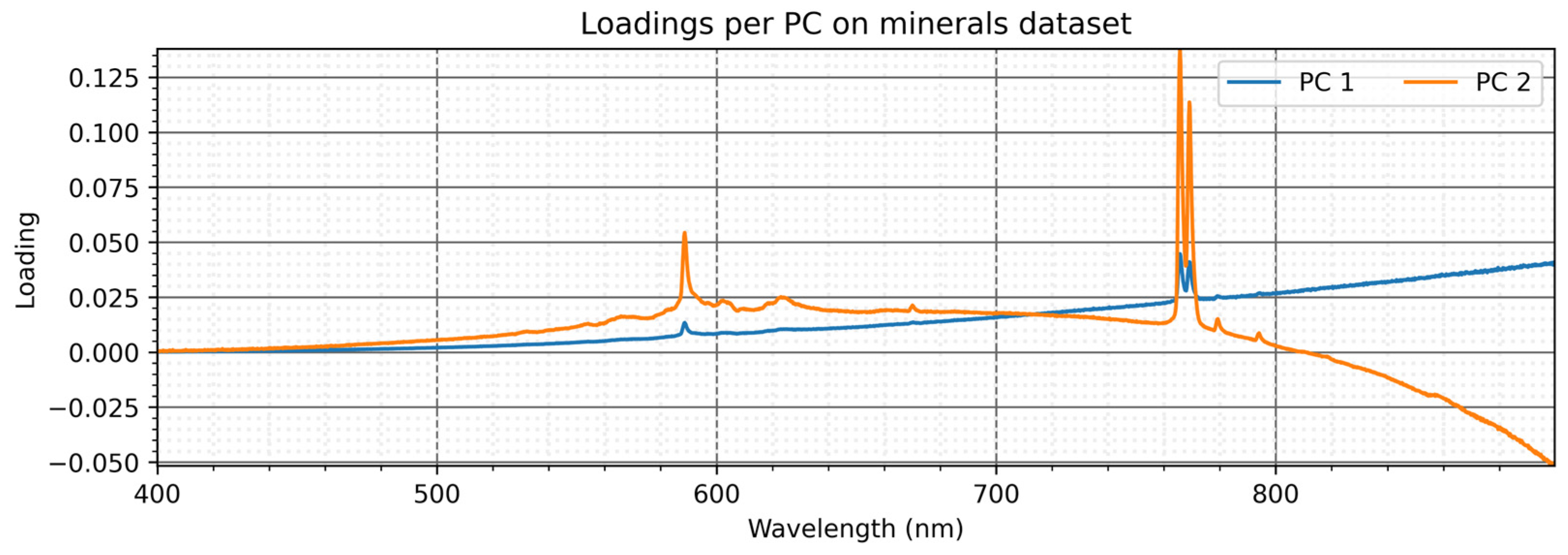
Additionally, when we look at the projection vectors (loadings) from this decomposition in Figure 6 for the non-standardized data, we observe that certain wavelengths have a stronger influence on the reduced representation. Specifically, for PC2, the wavelengths around 588 nm and 766–770 nm exhibit prominent peaks, suggesting that these spectral regions are particularly informative for differentiating mineral species. These wavelengths are commonly associated with elemental emissions, such as sodium and potassium lines, and iron oxide emissions which are relevant markers in high-temperature combustion analysis of sulfide minerals. In contrast, PC1 shows a more gradual loading distribution, with a slight increase in importance in the higher wavelengths (~800–900 nm), indicating a more general trend rather than sharp spectral features.

4.3. Classification Algorithms Evaluation

Table 3 lists the performance of the selected machine learning algorithms after applying the nested cross-validation strategy with hyperparameter search. For clarity, only the best-performing results per model are included. To evaluate each model’s performance and robustness, we report the BAcc and normal Acc metrics in training and testing sets. Precision, recall, and F1-score, both in average (macro) and weighted forms are also reported for the testing set. The weighted version uses the number of samples in each class to assign a weight compared to the total number of testing samples.
Among the tested models, the HB classifier delivered the best performance, achieving a BAcc of 98.5% ± 0.007 in training (note that the training and hyperparameter search is performed using nested CV, thus a standard deviation σ from the average BAcc can be calculated, as depicted in Table 3) and a test BAcc of 99.3%. This model consistently showed high precision, recall, and F1-scores, all around or above 99%, depicting its ability to model complex decision boundaries and interactions among spectral features. The weighted and average versions of these metrics further confirm its robustness across classes.
Random forest and SVM models also demonstrated competitive results. RF, using 50 estimators, achieved a BAcc of 97.7% in testing, closely followed by the SVM with a linear kernel and regularization parameter C = 1000, which obtained a BAcc 98.0% in testing. Notably, RF slightly edges out SVM in precision and recall, suggesting better handling of class-specific distinctions.
While DT and KNN models showed moderate performance, achieving a BAcc of 87.6% and 87.9%, respectively, in testing, they remain valuable for baseline comparisons due to their simplicity and interpretability. However, they exhibited lower recall and F1-scores, especially in the average (macro) versions, indicating reduced performance for less-represented classes.
In the context of the deep learning approaches, Table 4 summarizes the performance of the ANN and the 1D-CNN optimized architectures. After hyperparameter tuning using Hyperband, the 1D-CNN architecture emerged as the top-performing model. This model achieved a BAcc of 99.1% in training and a test BAcc of 99.0%. Precision, recall, and F1-score all reached 1.00 in their weighted forms, and 0.990 in the macro (average) versions, indicating consistency across all classes. Moreover, early stopping was triggered during training to prevent overfitting, as validated by the convergence of the loss function in the training and validation curves at 80 epochs for the ANN model and at 85 epochs for the 1D-CNN model.
Although the ANN model demonstrated lower generalization capacity with a testing balanced accuracy of 89.8%, and a macro averaged F1-score of 87.0%, representing a diminished performance particularly on underrepresented classes, the model serves as a baseline for evaluating the contribution of convolutional layers to feature extraction from spectral data.
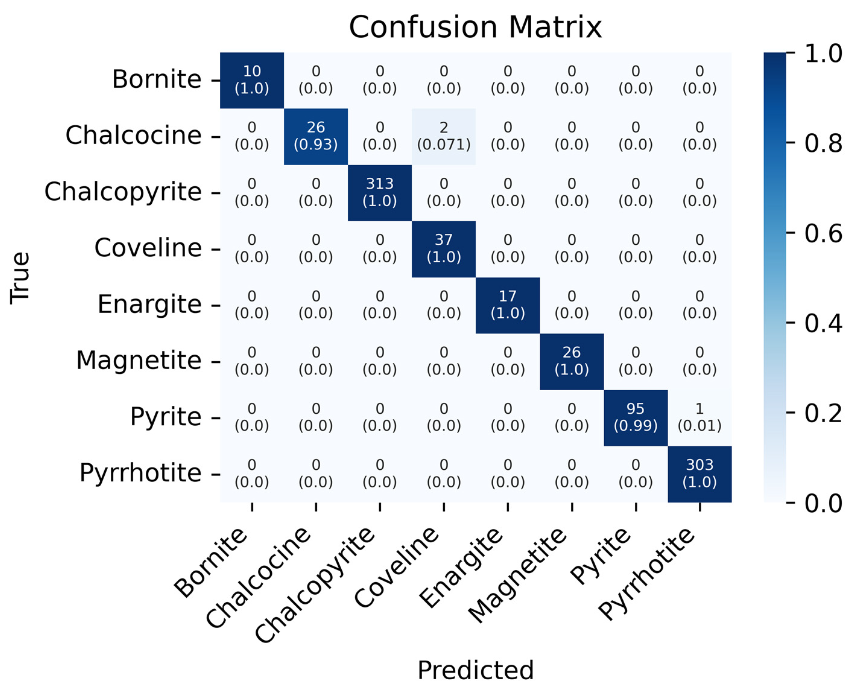
The confusion matrix for the 1D-CNN model on the test set is shown in Figure 7, illustrating the model’s capability to accurately classify spectral emissions across all eight mineral classes.
Most notably, from Figure 7, perfect classification was achieved for minerals such as bornite, chalcopyrite, coveline, enargite, magnetite, and pyrrhotite, with only a single misclassification observed in the case of pyrite and two misclassifications in the case of chalcocine, achieving a 93.0% and 99.0% true classification rate, respectively.
Finally, we conducted McNemar’s test to assess whether the performance differences between the models are statistically significant. This non-parametric test is specifically de-signed to evaluate paired nominal data and is commonly applied to classification tasks when comparing the predictions of two models on the same dataset.
As shown in Table 5, the 1D-CNN model significantly outperforms both the ANN and HB models. The comparison with ANN yields an extremely low p-value, indicating a highly significant difference in prediction behavior. While the difference between 1D-CNN and HB is less pronounced, it is still statistically significant (p = 7.149 × 10⁻³), confirming that even small improvements in balanced accuracy is meaningful because of the imbalanced nature of the dataset. Similarly, HB significantly outperforms ANN, further supporting the ranking of model performance.
In summary, the deep learning-based 1D-CNN model not only achieved better generalization on the test dataset but also demonstrated consistent performance across all classes and evaluation metrics when compared to traditional machine learning models. While the 1D-CNN approach is computationally more intensive and less inherently interpretable than models such as HB, its robust classification results and minimal misclassifications, confirmed through confusion matrix analysis and the statistical test, justify its selection as the most effective model for this task.

4.4. Discussion of the Optimized 1D-CNN Architecture

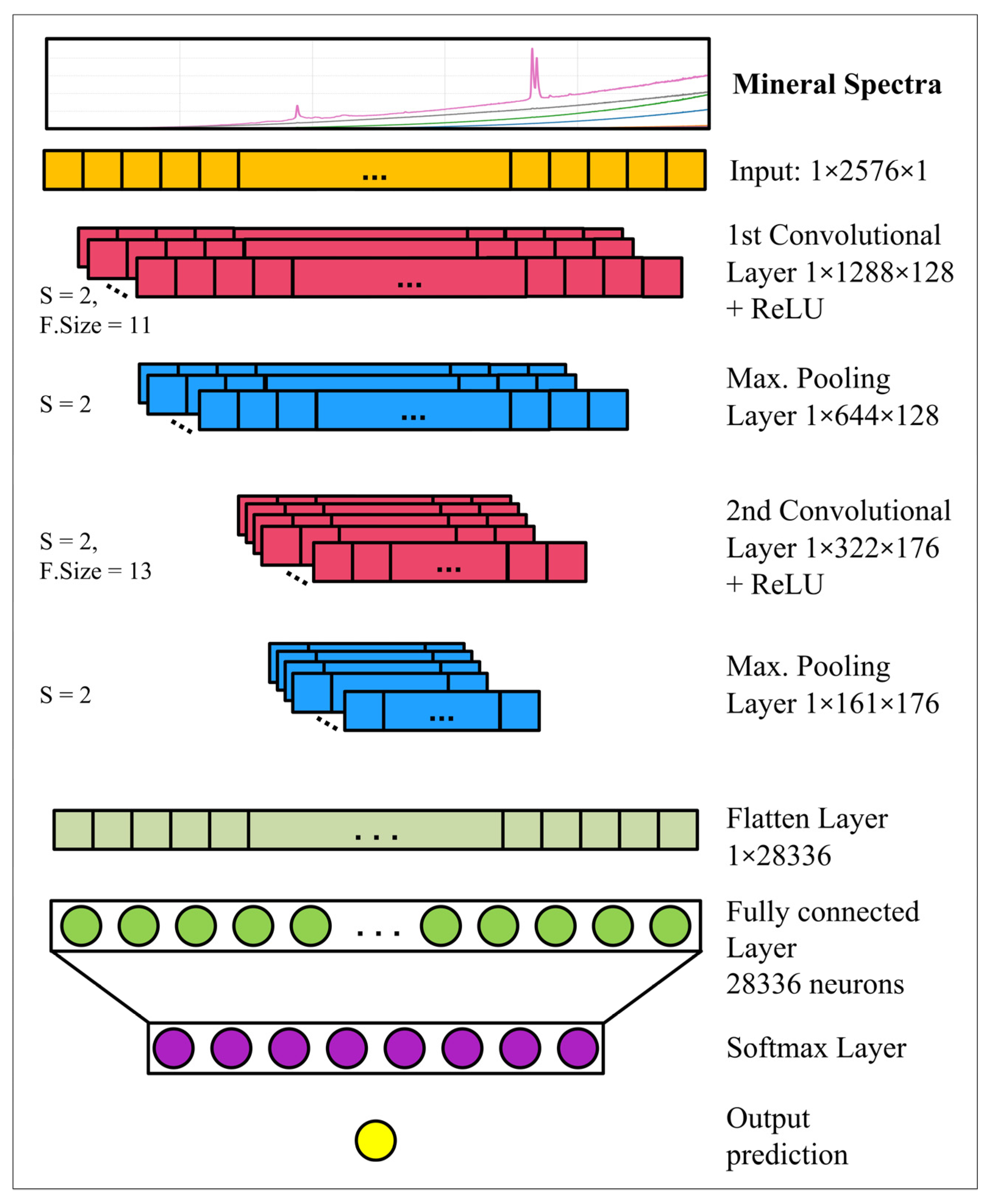
Figure 8 illustrates the full scheme of the optimized 1D-CNN architecture used for classifying mineral emission spectra. This model stands out not only for its high predictive performance, as previously discussed, but also for its simple design. The network consists of only two convolutional layers with a moderate number of filters and with relatively small sizes (11 and 13), followed by a standard fully connected layer. Similar achievements for spectral data can be found in the literature, for example, in [25], authors reported a 1D-CNN based model designed with two convolutional layers for feature extraction from NIR spectroscopy data in a remote sensing application.
This simple structure can be attributed to the nature of the spectral signals, which are continuous, smooth, and exhibit consistent trends with localized peaks (see Figure 4). These characteristics can reduce the need for deeper or more complex deep learning architectures. Moreover, compact 1D-CNNs like the one implemented here offer important practical benefits such as reduced training and inference time, and lower memory usage, in our case the model contains ~1.5 million total parameters (trainable and non-trainable) and can be stored in a keras file with a size of ~6.0 MB, this allows for an easier deployment in real-time or resource-constrained embedded hardware for industrial environments and applications. These advantages are consistent with the findings reported by Kiranyaz et al. [44], who emphasize the importance of compact CNN architectures in signal processing tasks where high classification accuracy must be balanced with computational efficiency. Their work highlights that shallow 1D-CNNs can achieve competitive performance, particularly in scenarios involving limited datasets or real-time constraints.

4.5. 1D-CNN Model Explainability

Figure 9 shows the results of applying the Grad-CAM method to our model and input spectra. The resulting heatmaps were normalized to the range from 0 to 1 and superimposed on the original spectral signals for enhanced interpretability. In this analysis, only the most informative examples are displayed, as the heatmaps for other mineral species revealed relatively uniform activation importance across all wavelengths. This uniformity may suggest that, for these species, the model is relying predominantly on the continuous spectral component rather than sharp emission peaks. One plausible explanation is that the spectral emission signatures from molecular or ionized species (e.g., Cu+, Fe2+, FeO, CuO) are either weaker or less well-resolved in those cases, leading the model to extract decision-relevant features from global spectral bands rather than specific spectral signatures.
In the case of pyrite (Figure 9a), the model highlights the significance of the spectral peaks and features around 600 and ~780 nm, which chemically correspond to iron oxides such as FeO and iron emission lines, along with sodium and potassium, as reported in [22]. This was also depicted in the PCA analysis in Figure 6. The identification of these features is crucial in industrial operations, as they are associated with good combustion quality and the optimization of resources such as oxygen-enriched air supply. For chalcopyrite (Figure 9b) and pyrrhotite (Figure 9c), the activation importance is more gradually distributed, suggesting that the model relies on wider spectral bands rather than distinct peaks to make predictions. In the specific case of chalcopyrite, its combustion under the experimental temperatures used in this study can lead to the formation of copper oxides such as CuO. These oxides are known to emit characteristic spectral features within the 580–720 nm range [45]. This emission behavior is moderately captured by the Grad-CAM activation in Figure 9b, particularly around the 550 nm region, suggesting that the model can detect and use this weak spectral emission during classification.

4.6. Limitations and Future Resarch Directions

Despite the strong performance metrics achieved in this study, some limitations must be acknowledged. First, although cross-validation and hyperparameter optimization strategies were employed to mitigate overfitting, deep learning models such as 1D-CNNs are inherently prone to overfit, especially when trained on relatively small and unbalanced datasets. This risk may increase when transferring models to new experimental conditions or industrial environments. Model generalization across unseen mineral species, presence of impurities, or different furnace types will be systematically evaluated in future studies. Additionally, to address the inherent variability in industrial ore feeds, future work will also explore model robustness in the presence of mixed-phase compositions. This includes expanding the dataset to include a wider range of sulfide minerals relevant for the copper industry, as well as mineral mixtures and copper concentrates.
Domain adaptation strategies and transfer learning approaches will be investigated to extend the applicability of the model to new datasets with minimal retraining. In addition, synthetic data generation using physics-based simulations or generative models could serve to augment the dataset and simulate realistic industrial conditions, thus enhancing model resilience to operational variability.
In addition, in industrial pyrometallurgical processes involving copper or iron sulfides and blended materials, it is highly desirable to estimate key indicators such as copper content or slag composition. In this context, the trained classification model could be adapted into a pretrained network for regression tasks, enabling the prediction of process-relevant variables directly from spectral data. Furthermore, integrating multi-sensor fusion techniques and combining spectral inputs with additional process variables such as oxygen enrichment or feed rates, could enhance predictive performance and provide a more comprehensive and robust analysis of the underlying metallurgical processes.
Another limitation concerns the long-term calibration drift of spectrometers, which may impact measurement consistency and reproducibility over extended periods. To address this, future research will include calibration stability assessments during the deployment of the sensing system in industrial environments, with the goal of establishing recalibration protocols.
Finally, future research will focus on integrating the 1D-CNN model into real-time monitoring systems in pyrometallurgical applications in the copper extractive industry. Additional interpretability studies will be conducted to validate the correspondence between the features activated by the deep learning model and known mineralogical characteristics from the mineral samples.

5. Conclusions

This study presents a machine learning and deep learning modeling approach for the VIS-NIR spectral data classification acquired from the emitted radiation from mineral sulfides in simulated flash combustion conditions. The best performance was achieved with a 1D-CNN model, which exhibited a classification balanced accuracy score of 99.0% on the test set. By looking at all the evaluated metrics, the optimized 1D-CNN model consistently outperformed traditional machine learning algorithms approaches, highlighting the suitability of convolutional architectures for spectral pattern recognition.
To enhance model explainability, Grad-CAM was applied to identify the spectral regions that significantly contributed to classification decisions. The results indicate that the model distinguished significant spectral peaks and features for pyrite, chalcopyrite, and pyrrhotite, providing insights into the physical and chemical basis of the classification process. These findings support the potential industrial application of deep learning towards real-time spectral monitoring in flash smelting processes, where the combustion quality is critical for efficiency and resource allocation.
Finally, this work contributes to the broader research community by introducing a publicly available labeled dataset of VIS-NIR emission spectra acquired under high-temperature conditions in a laboratory scale setup. This dataset represents a novel resource for benchmarking spectral classification techniques under conditions relevant to metallurgical applications. By enabling open access to the data and describing the experimental procedures in detail, we aim to promote reproducibility, comparative analysis, and the development of more robust and generalizable models in future research.

Author Contributions

Conceptualization, C.T. (Carlos Toro) and W.D.; methodology, C.T. (Carlos Toro), W.D. and G.R.; software, C.T. (Carlos Toro); validation, C.T. (Carlos Toro) and E.B.; formal analysis, C.T. (Carlos Toro), N.C. and C.T. (Carla Taramasco); investigation, C.T. (Carlos Toro), M.P. and G.R.; resources, E.B. and C.T. (Carla Taramasco); data curation, C.T. (Carlos Toro) and M.P.; writing—original draft preparation, W.D., P.O.-A. and M.P.; writing—review and editing, C.T. (Carlos Toro), N.C., P.O.-A. and C.T. (Carla Taramasco); visualization, C.T. (Carlos Toro) and G.R.; supervision, E.B.; project administration, G.R.; funding acquisition, E.B. and C.T. (Carlos Toro). All authors have read and agreed to the published version of the manuscript.

Funding

This research was funded by the CONICYT, Anillo Minería ACM170008, and by FONDEF IT under Grant Number 16M10029. The work of Carlos Toro was supported in part by the CONICYT Fondecyt/Postdoctorate grant under Project number 3170897.

Data Availability Statement

The dataset collected in this research is published online and can be accessed here: https://doi.org/10.6084/m9.figshare.28473440.v1. The folder contains all the analyzed spectral signals and data were saved in Numpy file format “.npy”.

Acknowledgments

We thank the Metallurgical Engineering Department at the University of Concepción for providing access to their facilities, which allowed us to conduct the experiments reported in this work.

Conflicts of Interest

The funders had no role in the design of the study; in the collection, analyses, or interpretation of data; in the writing of the manuscript; or in the decision to publish the results.

Abbreviations

The following abbreviations are used in this manuscript:
VISVisible
NIRNear-Infrared
1D-CNNOne-dimensional Convolutional Neural Network
Grad-CAM Gradient-weighted Class Activation Mapping
FTIRFourier Transform Infrared
PCAPrincipal Component Analysis
AdamAdaptive Moment Estimation
SNRSignal-to-Noise-Ratio
ANNArtificial Neural Network
KNNK-Nearest Neighbors
SVMSupport Vector Machine
DTDecision Tree
HBHistogram Boosting
RFRandom Forest
RAMRandom Access Memory
CPUCentral Processing Unit
GPUGraphics Processing Unit
CVCross-Validation
AccAccuracy
BAccBalanced Accuracy

References

  1. Schlesinger, M.E.; Sole, K.C.; Davenport, W.G.I.; Flores, G.R.F.A. Extractive Metallurgy of Copper; Elsevier: Amsterdam, The Netherlands, 2021. [Google Scholar] [CrossRef]
  2. Davenport, W.G.; Jones, D.M.; King, M.J.; Partelpoeg, E.H. Flash Smelting: Analysis, Control and Optimization, 2nd Revised ed.; Wiley-Tms: Warrendale, PA, USA, 2004. [Google Scholar]
  3. Bacedoni, M.; Moreno-Ventas, I.; Ríos, G. Copper Flash Smelting Process Balance Modeling. Metals 2020, 10, 1229. [Google Scholar] [CrossRef]
  4. Kemori, N.; Ojima, Y.; Kondo, Y. Variation of the Composition and Size of Copper Concentrate Particles in the Reaction Shaft. In Proceedings of the Flash Reaction Processes; Center for Pyrometallurgy Conference, University of Missouri-Rolla: Rolla, MO, USA; University of Utah: Salt Lake City, UT, USA, 1988; pp. 47–68. [Google Scholar]
  5. Jokilaakso, A.; Suominen, R.; Pekka, T.; Lilius, K. Oxidation of Chalcopyrite in Simulated Suspension Smelting Conditions. Trans. Instit. Min. Metall.(Sect. C Mineral Process. Extr. Metall.) 1991, 100, C79–C90. [Google Scholar]
  6. Ahokainen, T.; Jokilaakso, A.; Vaarno, J.; Jarvi, J. Modelling Chalcopyrite Combustion Together with Fluid Flow Simulation. In Proceedings of the International Conference on CFD in the Mineral & Metal Processing and Power Generation, Melbourne, Australia, 3–4 July 1997; pp. 213–221. [Google Scholar]
  7. Pérez-Tello, M.; Parra, V.; Sánchez, V.; Gómez, A.; Brown, F.; Parra, R.; Balladares, E.; Araneda, E. Evolution of Size and Chemical Composition of Copper Concentrate Particles Oxidized Under Simulated Flash Smelting Conditions. Met. Mater. Trans. B 2018, 49, 627–643. [Google Scholar] [CrossRef]
  8. Jorgensen, F.R.A. Combustion of Pyrite Concentrate under Simulated Flash-Smelting Conditions. Trans. Inst. Mining Metall. 1981, 90, C1–C9. [Google Scholar]
  9. Jorgensen, F.R.A. Single-Particle Combustion of Chalcopyrite. Proc. Australas. Inst. Min. Metall. 1983, 288, 37–46. [Google Scholar]
  10. Jorgensen, F.R.A.; Moyle, F.J.; Wadsley, M.W. Structural Changes Associated with the Ignition of Pyrite and Chalcopyrite during Flash Smelting. In Process Mineralogy IX: Applications to Mineral Beneficiation, Metallurgy, Gold, Diamonds, Ceramics, Environment and Health; Minerals, Metals & Materials Society: Warrendale, PA, USA, 1989; pp. 323–341. [Google Scholar]
  11. Kemori, N.; Akada, A.; Kondo, Y. Development of a Concentrate Burner for Industrial Oxygen Flash Smelting. In Copper 91, Pyrometallurgy of Copper; Pergamon Press: Oxford, UK, 1991; pp. 141–154. [Google Scholar]
  12. Chen, H.R.; Mei, C.; Xie, K.; Li, X.; Zhou, J.; Wang, X.; Ge, Z. Operation Optimization of Concentrate Burner in Copper Flash Smelting Furnace. Trans. Nonferrous Met. Soc. China 2004, 14, 631–636. [Google Scholar]
  13. Jorgensen, F.R.A.; Campbell, A.; Taylor, R.; Washington, B. Sampling and Measurements in the Reaction Shaft at Olympic Dam. In Proceedings of the First Extractive Metallurgy Operators’ Conference, Melbourne, Australia, 7–8 November 2005; pp. 87–93. [Google Scholar]
  14. Parada, R.; Parra, R.; Wilkomirsky, I. Dynamic Simulation of a Flash Furnace. Can. Metall. Q. 2004, 43, 561–569. [Google Scholar] [CrossRef]
  15. Solnordal, C.B.; Jorgensen, F.R.A.; Koh, P.T.L.; Hunt, A. CFD Modelling of the Flow and Reactions in the Olympic Dam Flash Furnace Smelter Reaction Shaft. Appl. Math. Model. 2006, 30, 1310–1325. [Google Scholar] [CrossRef]
  16. Jorgensen, F.R.A.; Zuiderwyk, M. Two-Colour Pyrometer Measurement of the Temperature of Individual Combusting Particles. J. Phys. E Sci. Instrum. 1985, 18, 486. [Google Scholar] [CrossRef]
  17. Tuffrey, N.E.; Richards, G.G.; Brimacombe, J.K. Two-Wavelength Pyrometry Study of the Combustion of Sulfide Minerals: Part I. Apparatus and General Observations. Metall. Materi. Trans. B 1995, 26, 929–942. [Google Scholar] [CrossRef]
  18. Morgan, G.J.; Brimacombe, J.K. Kinetics of the Flash Converting of MK (Chalcocite) Concentrate. Met. Mater. Trans B 1996, 27, 163–175. [Google Scholar] [CrossRef]
  19. Laurila, T.; Hernberg, R.; Oikari, R.; Joutsenoja, T.; Mikkola, P.; Ranki-Kilpinen, T.; Taskinen, P. Pyrometric temperature and size measurements of chalcopyrite particles during flash oxidation in a laminar flow reactor. Metall. Materi. Trans. B 2005, 36, 201–208. [Google Scholar] [CrossRef]
  20. Reyes, G. Desarrollo y Aplicación de un Sensor Optoelectrónico Para el Monitoreo de la Operación de un Horno de Fusión Flash de Concentrados de Cobre. Ph.D. Thesis, Universidad de Concepción, Concepción, Chile, 2021. Available online: https://repositorio.udec.cl/items/189dfe19-e58e-4aae-a714-e032da37799f (accessed on 12 May 2025).
  21. Díaz, W.; Toro, C.; Balladares, E.; Parra, V.; Coelho, P.; Reyes, G.; Parra, R. Spectral Characterization of Copper and Iron Sulfide Combustion: A Multivariate Data Analysis Approach for Mineral Identification on the Blend. Metals 2019, 9, 1017. [Google Scholar] [CrossRef]
  22. Toro, C.; Torres, S.; Parra, V.; Fuentes, R.; Castillo, R.; Díaz, W.; Reyes, G.; Balladares, E.; Parra, R. On the Detection of Spectral Emissions of Iron Oxides in Combustion Experiments of Pyrite Concentrates. Sensors 2020, 20, 1284. [Google Scholar] [CrossRef] [PubMed]
  23. Jahoda, P.; Drozdovskiy, I.; Payler, S.J.; Turchi, L.; Bessone, L.; Sauro, F. Machine learning for recognizing minerals from multispectral data. Analyst 2021, 146, 184–195. [Google Scholar] [CrossRef]
  24. Es-sahly, S.; Elbasbas, A.; Naji, K.; Lakssir, B.; Faqir, H.; Dadi, S.; Rabie, R. NIR-Spectroscopy and Machine Learning Models to Pre-concentrate Copper Hosted Within Sedimentary Rocks. Min. Metall. Explor. 2024, 41, 1979–1995. [Google Scholar] [CrossRef]
  25. Kok, M.; Sarjant, S.; Verweij, S.; Vaessen, S.F.C.; Ros, G.H. On-site soil analysis: A novel approach combining NIR spectroscopy, remote sensing and deep learning. Geoderma 2024, 446, 116903. [Google Scholar] [CrossRef]
  26. Smith, R.; Spano, T.L.; McDonnell, M.; Drane, L.; Gibbs, I.; Miskowiec, A.; Niedziela, J.L.; Shields, A.E. Interpretable Machine Learning Models Classify Minerals, Spectroscopy. Sci. Rep. 2025, 15, 15807. [Google Scholar] [CrossRef]
  27. Bernicky, A.R.; Davis, B.; Kadiyski, M.; Loock, H.-P. Mineralogical Analysis of Solid-Sample Flame Emission Spectra by Machine Learning. Anal. Chem. 2024, 96, 19330–19338. [Google Scholar] [CrossRef]
  28. Yang, B.; Yang, Z.; Xu, Y.; Cheng, W.; Zhong, F.; Ye, D.; Weng, H. A 1D-CNN model for the early detection of citrus Huanglongbing disease in the sieve plate of phloem tissue using micro-FTIR. Chemom. Intell. Lab. Syst. 2024, 252, 105202. [Google Scholar] [CrossRef]
  29. Li, X.; Wu, J.; Bai, T.; Wu, C.; He, Y.; Huang, J.; Li, X.; Shi, Z.; Hou, K. Variety classification and identification of jujube based on near-infrared spectroscopy and 1D-CNN. Comput. Electron. Agric. 2024, 223, 109122. [Google Scholar] [CrossRef]
  30. Sang, X.; Zhou, R.; Li, Y.; Xiong, S. One-Dimensional Deep Convolutional Neural Network for Mineral Classification from Raman Spectroscopy. Neural Process. Lett. 2022, 54, 677–690. [Google Scholar] [CrossRef]
  31. Qi, Y.; Hu, D.; Zheng, M.; Jiang, Y.; Chen, Y.P. Deep learning assisted Raman spectroscopy for rapid identification of 2D materials. Appl. Mater. Today 2024, 41, 102499. [Google Scholar] [CrossRef]
  32. Contreras, J.; Bocklitz, T. Explainable artificial intelligence for spectroscopy data: A review. Pflug. Arch. Eur J Physiol. 2024, 477, 603–615. [Google Scholar] [CrossRef]
  33. Beć, K.; Grabska, J.; Huck, C. Interpretability in near-infrared (NIR) spectroscopy: Current pathways to the long-standing challenge. TrAC-Trend. Anal. Chem. 2025, 189, 118254. [Google Scholar] [CrossRef]
  34. Xia, J.; Li, J.; Wang, X.; Li, Y.; Li, J. Enhanced cancer classification and critical feature visualization using Raman spectroscopy and convolutional neural networks. Spectrochim. Acta A Mol. Biomol. Spectrosc. 2025, 326, 125242. [Google Scholar] [CrossRef]
  35. Selvaraju, R.R.; Cogswell, M.; Das, A.; Vedantam, R.; Parikh, D.; Batra, D. Grad-CAM: Visual Explanations from Deep Networks via Gradient-Based Localization. In Proceedings of the 2017 IEEE International Conference on Computer Vision (ICCV), Venice, Italy, 22–29 October 2017; pp. 618–626. [Google Scholar] [CrossRef]
  36. Shi, G.-Y.; Wu, H.-P.; Luo, S.-H.; Lu, X.-Y.; Ren, B.; Zhang, Q.; Lin, W.-Q.; Chen, R.-Y.; Guo, P.; Chen, H.-B.; et al. 1D Gradient-Weighted Class Activation Mapping, Visualizing Decision Process of Convolutional Neural Network-Based Models in Spectroscopy Analysis. Anal. Chem. 2023, 95, 9959–9966. [Google Scholar] [CrossRef]
  37. Wang, X.; Ni, L.; Zhang, C.; Xu, Q.; Ye, S. Using a one-dimensional convolutional neural network on FTIR spectroscopy to measure the thickness of composite plastic films. Infrared Phys. Technol. 2025, 147, 105777. [Google Scholar] [CrossRef]
  38. Szeghalmy, S.; Fazekas, A. A Comparative Study of the use of Stratified Cross-Validation and Distribution-Balanced Stratified Cross-Validation in Imbalanced Learning. Sensors 2023, 23, 2333. [Google Scholar] [CrossRef] [PubMed]
  39. Li, L.; Jamieson, K.; DeSalvo, G.; Rostamizadeh, A.; Talwalkar, A. Hyperband: A Novel Bandit-Based Approach to Hyperparameter Optimization. J. Mach. Learn. Res. 2018, 18, 1–52. [Google Scholar]
  40. Zeng, F.; Peng, W.; Kang, G.; Feng, Z.; Yue, X. Spectral Data Classification by One-Dimensional Convolutional Neural Networks. In Proceedings of the 2021 IEEE International Performance, Computing, and Communications Conference (IPCCC), Austin, TX, USA, 29–31 October 2021. [Google Scholar] [CrossRef]
  41. Kingma, D.P.; Ba, J. Adam: A method for stochastic optimization. arXiv 2014. [Google Scholar] [CrossRef]
  42. Toro, C. Dataset of Spectral Emission of Mineral Species during Combustion. Figshare Dataset 2025. [Google Scholar] [CrossRef]
  43. Kokaly, R.F.; Clark, R.N.; Swayze, G.A.; Livo, K.E.; Hoefen, T.M.; Pearson, N.C.; Wise, R.A.; Benzel, W.M.; Lowers, H.A.; Driscoll, R.L.; et al. USGS Spectral Library Version 7 Data: U.S. Geological Survey Data Release; U.S. Geological Survey Data Release: Reston, VA, USA, 2017. [CrossRef]
  44. Kiranyas, S.; Abdeljaber, O.; Avci, O.; Gabbouj, M. 1-D Convolutional Neural Networks for Signal Processing Applications. In Proceedings of the 2019 IEEE International Conference on Acoustics, Speech and Signal Processing (ICASSP), Brighton, UK, 12–17 May 2019. [Google Scholar] [CrossRef]
  45. Gole, J.L. Toward the Modeling of the Oxidation of Small Metal and Metalloid Molecules. In Gas Phase Metal Reactions; Elsevier: Amsterdam, The Netherlands, 1992; pp. 573–604. ISBN 978-0-444-89070-2. [Google Scholar]
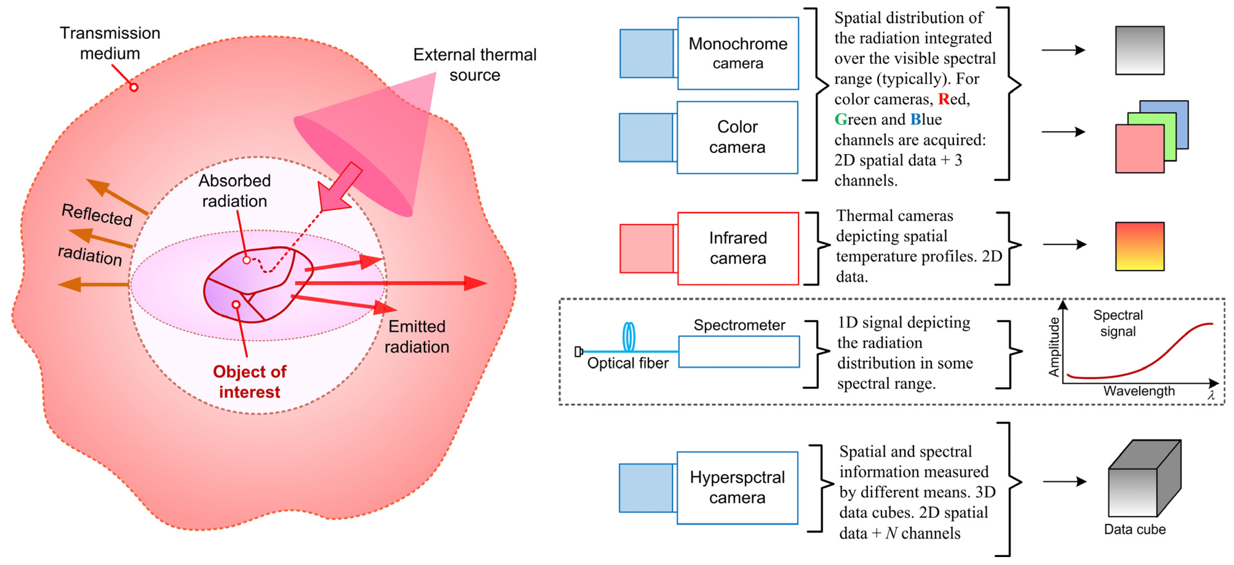
Figure 1. Typical radiometric measurement technologies and modalities, including spectroscopy and imaging methods.
Bdcc 09 00130 g001
Figure 2. Experimental setup for particulate sulfide minerals combustion.
Bdcc 09 00130 g002
Figure 3. General acquisition and modeling methodology.
Bdcc 09 00130 g003
Figure 4. Average emission spectra (a) all mineral spectra profiles and (b) mineral spectra with lower intensities.
Bdcc 09 00130 g004
Figure 5. Reduced representation of spectral data by applying PCA, score plot for principal components 1 and 2 of (a) raw data and (b) standardized data.
Bdcc 09 00130 g005
Figure 6. Loading vector from PCA decomposition for PC 1 and PC 2.
Bdcc 09 00130 g006
Figure 7. Confusion matrix with normalized values and per-class counts, illustrating correct and misclassified instances for the optimized 1D-CNN model on the test set.
Bdcc 09 00130 g007
Figure 8. 1D-CNN optimized architecture for minerals emission spectra classification.
Bdcc 09 00130 g008
Figure 9. 1D-CNN model interpretability by using Grad-CAM for different species, (a) heatmap interpretability for pyrite, (b) heatmap interpretability for chalcopyrite, (c) heatmap interpretability for pyrrhotite.
Bdcc 09 00130 g009
Table 2. Hyperparameter search space values for implemented machine learning models.
ModelHyperparametersValues
KNNK (n_neighbors)1 to 15
Distance metrics (metric)Minkowski, euclidian, manhattan, cosine
SVMKernel function (kernel) Linear, radial basis function (rbf), polynomial (poly), sigmoid
Regularization (C)1, 10, 100, 1000
Class Weight (class_weight) Balanced, None
GammaScale, auto, 2
DTMax depth5, 10, 15
Max leaf nodes (max_leaf_nodes)2 to 20 with steps of 2
Min samples leaf (min_samples_leaf)1 to 10 with steps of 2
Min samples split (min_samples_split)2 to 10 with steps of 2
Impurity measure (criterion)Entropy, gini
HBMaximum number of iterations (max_iter)50, 100, 150
RFN° estimators (n_estimators)10, 20, 50
Note: For each hyperparameter, the name used by Scikit-learn is depicted in parentheses to facilitate reproducibility.
Table 3. Comparison of Trained Classification Algorithms with a machine learning approach.
ModelOptimal HyperparametersAcc/BAcc (± σ)
in Train
Acc/BAcc
in Test
Precision
a/w * in Test
Recall
a/w * in Test
F1-Score
a/w * in Test
KNNK = 3 neighbors
Distance metric: Minkowski
0.878/
0.884 ± 0.010
0.864/0.8790.874/0.9130.879/0.8640.811/0.848
SVMLinear kernel
Regularization: C = 1000
0.998/
0.983 ± 0.004
0.983/0.9800.987/0.9830.980/0.9830.983/0.982
DTMax depth = 10
Max leaf nodes = 16
Min samples leaf = 7
Min samples split = 10
Impurity measure: Entropy
0.945/
0.886 ± 0.016
0.914/0.8760.887/0.9250.886/0.9200.878/0.917
HBMax iter = 1000.999/
0.985 ± 0.006
0.993/0.9820.991/0.9930.982/0.9930.986/0.993
RFN° estimators = 500.999/
0.973 ± 0.009
0.989/0.9770.984/0.9890.977/0.9890.980/0.989
* a/w: average and weighted versions of the metrics among all the classes. Accuracy in training is calculated only after the nested CV strategy and using the model with best hyperparameters.
Table 4. Comparison of Optimized Neural Networks Based Models for Spectra Classification.
ModelOptimal HyperparametersTraining
Acc/BAcc
Testing
Acc/Bacc
Precision
a/w in Test
Recall
a/w in Test
F1-Score
a/w in Test
ANNN° hidden layers = 3
Neurons per layer = {640, 1408, 1920}
Activation function = ReLu
Learning rate = 0.0001
0.978/0.8990.961/0.8980.880/0.9600.860/0.9600.870/0.960
1D-CNNN° conv. layers = 2
N° filters per layer = {128, 176}
Filters size per layer = {11, 13}
Stride = 2 for all layers
Learning rate = 0.0001
Activation function = ReLu
0.997/0.9910.996/0.9900.990/1.000.990/1.000.990/1.00
Table 5. Statistical Comparison of Models’ Performance using McNemar’s Test.
Model PairBAcc DifferenceMcNemar’s Test (p-Value) *
1D-CNN vs ANN0.0924.336 × 10−63
1D-CNN vs HB0.0085.152 × 10−3
HB vs ANN0.0847.521 × 10−57
* McNemar’s test was applied using confusion matrices estimated from reported balanced accuracy, under the assumption of a 13% positive classes (less represented minerals) and 87% negative class distribution (pyrite, chalcopyrite and pyrrhotite).
Disclaimer/Publisher’s Note: The statements, opinions and data contained in all publications are solely those of the individual author(s) and contributor(s) and not of MDPI and/or the editor(s). MDPI and/or the editor(s) disclaim responsibility for any injury to people or property resulting from any ideas, methods, instructions or products referred to in the content.