Article

Robust Anomaly Detection of Multivariate Time Series Data via Adversarial Graph Attention BiGRU

1
Guangdong Provincial Key Laboratory of Precision Equipment and Manufacturing Technology, School of Mechanical and Automotive Engineering, South China University of Technology, Guangzhou 510641, China
2
Shanxi Information Industry Technology Research Institute Company Ltd., Taiyuan 030032, China
*
Author to whom correspondence should be addressed.
Big Data Cogn. Comput. 2025, 9(5), 122; https://doi.org/10.3390/bdcc9050122
Submission received: 18 March 2025 / Revised: 23 April 2025 / Accepted: 6 May 2025 / Published: 8 May 2025

Abstract

Multivariate time series data (MTSD) anomaly detection due to complex spatio-temporal dependencies among sensors and pervasive environmental noise. The existing methods struggle to balance anomaly detection accuracy with robustness against data contamination. Hence, this paper proposes a robust multivariate temporal data anomaly detection method based on graph attention for training convolutional neural networks (PGAT-BiGRU-NRA). Firstly, the parallel graph attention (PGAT) mechanism extracts the time-dependent and spatially related features of MTSD to realize the MTSD fusion. Then, a bidirectional gate recurrent unit (BiGRU) is utilized to extract the contextual information of the data to avoid information loss. In addition, reconstructing the noise for adversarial training aims to achieve a more robust anomaly detection of MTSD. The experiments conducted on real industrial equipment datasets evaluate the effectiveness of the method in the task of MTSD, and the comparative experiments verify that the proposed method outperforms the mainstream baseline model. The proposed method achieves anomaly detection and robust performance in noise interference, which provides feasible technical support for the stable operation of industrial equipment in complex environments.

1. Introduction

In recent years, the rapid development of emerging technologies, such as the Internet of Things (IoT), cloud computing, and 6G, has led to explosive growth in data size and highly complex data patterns in healthcare [1], aerospace [2], manufacturing [3], and cybersecurity [4]. The sensor samples and records form a time series of data (TSD) according to time correlation, using the progression of the variable of interest over time or at irregular intervals. Timing data reflect the real-time state of the system due to the complexity of the sensor operating environment, the inherent characteristics of the sensor itself, and the imbalance of system resources and other interferences [5]. Thus, there are irregular fluctuations in the real-time collection of data that are not anomalies. Consequently, there has been growing attention on developing data processing methods that can adequately extract time series data letter features and effectively improve the accuracy and real-time performance of identifying abnormal behaviors in recent years [6].
TSD relies on time-lapse, which contains a large amount of information with many features that are difficult to achieve through manual labeling. Moreover, unsupervised feature learning is an effective way to analyze time series data. For example, support vector regression (SVR) [7] employs time-lag coordinate autoregression and phase space reconstruction to extract temporal data features for prediction and to verify the prediction accuracy with wind speed data. Time series forest (TSF) [8] constructs a collection of tree systems for time series data to randomly extract sampling features and linear relationships at each tree node and combines entropy gain and distance metrics to evaluate the effectiveness of the model. Given the complex and highly dynamic characteristics of physical equipment systems in the era of artificial intelligence (AI), relying solely on single-dimensional time series data may result in vulnerability to noise interference, leading to insufficient model robustness. Hence, multiple sensors are required to provide more comprehensive information, monitor equipment anomalies, and predict anomalies to prevent uncontrollable events.
To avoid incorrectly identifying normal fluctuations in timing data as anomalies, the correlation between different variables of the anomaly detection of multivariate time series data (MTSD) is used to satisfy the detection performance in multidimensional timing data patterns. Deep learning methods [9] are extremely capable of handling complex correlations of MTSD with nonlinear properties to mine high-dimensional data features. Furthermore, unsupervised reconstruction methods [10] are developed for MTSD anomaly detection in practical applications. However, existing research mainly focuses on specific scenarios, lacking a comprehensive approach to satisfy the data pattern complexity and detection accuracy robustness of MTSD. Therefore, there is an urgent need for an unsupervised deep learning-based MTSD processing method that fully exploits temporal dependencies and spatial correlations of the nodes, improves detection accuracy, and maintains the robustness of the detection.
Currently, MTSD processing is limited by the uncertainty and complexity of industrial data. The issues are summarized as follows:
(1)
Existing MTSD typically use dimension shifting and scaling to eliminate data size, increasing training speed. However, due to the inconsistent influence of different dimensional data on the results, failure to fully consider the spatial correlation characteristics between different dimensional data leads to inadequate model performance [11]. However, due to the complex change patterns of MTSD and the inclusion of both continuous and discrete variables, it is difficult to make the model compatible with historical data and the current task, while adequately extracting spatially relevant features. Thus, the optimal scheme for compatible hybrid temporal and spatial feature extraction has yet to be investigated.
(2)
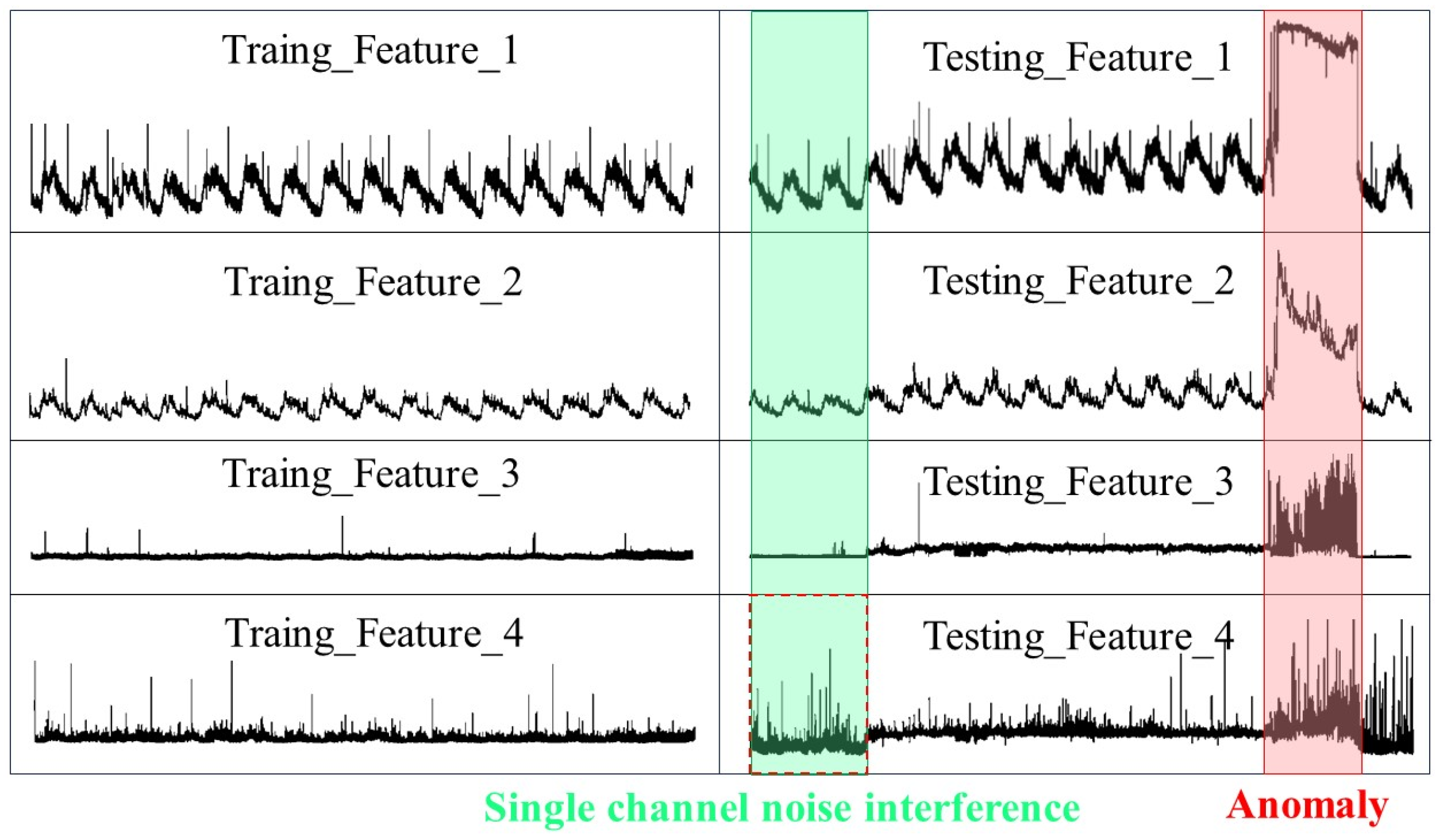
Extracting potential representations from MTSD is susceptible to noise interference and fluctuations in the training set. As shown in Figure 1 (green indicates fluctuation, red indicates abnormality), the collected data contain a significant amount of noise, visualizing considerable noise in a real dataset, which is a common phenomenon in the real world. Existing methods lack the robustness to deal with MTSD in the face of noise and anomalous contamination. Hence, it is difficult for the model to achieve the expected results due to large errors caused by noise and interference during data reconstruction.
In summary, although MTSD can provide more comprehensive information, the existing MTSD anomaly detection is highly susceptible to noise and anomaly interference. Moreover, no research has been focused on the highly robust processing of MTSD, according to the survey. This paper proposes a processing method compatible with extracting MTSD temporal and spatial features to realize data fusion and add noise against training to improve robustness. The contributions of this paper are summarized as follows:
(1)
A parallel improved graph attention (PGAT) is proposed to analyze temporal dependence and spatial correlation in MTSD without any prior knowledge, thereby avoiding misclassification of normal fluctuations as anomalies.
(2)
Integrating deep learning technology, BiGRU model is selected to learn the spatio-temporal features of dimensional time series data. In addition, the context-dependent features are obtained to prevent information loss and enhance the robust performance of the model.
(3)
The advantages of predictive and reconstructive models are combined by introducing joint optimization. The reconstructed noise samples are used for adversarial training to improve the robustness of the model in the face of contaminated data. The performance and explanatory power of the model are tested on three public datasets, proving that the proposed method outperforms eight typical baseline models. Finally, the proposed model is applied to anomaly detection in laboratory equipment, validating the effectiveness of the method.
The rest of the paper is organized as follows: Section 2 reviews the related work on multidimensional time series data fusion and robust anomaly detection processing. Section 3 introduces the proposed PGAT-BiGRU-NRA model and provides a detailed description of the main modules. Section 4 conducts experiments and provides experimental results to evaluate the model. Finally, Section 5 concludes this article.

2. Related Work

2.1. MTSD Fusion

Multivariate data can provide more comprehensive information than univariate data, eliminating the effects of instability and susceptibility to noise interference of univariate data by complementing each other’s support. This robust characterization enhances the accuracy of information extraction [12]. Data fusion technology effectively improves the processing capability and utilization rate of time series big data. Moreover, it integrates, correlates, and analyzes noisy massive high-dimensional multivariate data and provides reliable and high-quality data support for subsequent anomaly detection prediction and decision-making [13]. Currently, commonly used data fusion methods can be categorized into probability-based fusion methods, D-S evidence theory-based fusion methods, knowledge-based fusion methods, and attention mechanism-based fusion methods. Table 1 summarizes data fusion methods based on probability, D-S evidence theory, and knowledge.
The attention mechanism is first applied to the vision domain [22] based on the idea of weight allocation, which assigns weights according to the importance of the observation features to focus on the important information and enhance the data processing capability of the model. The multi-head self-attention mechanism [23] learns multiple caveats through various heads. Each head can sense contextual information to extract external discriminative features, improving the self-attention mechanism. However, it comes with computational complexity and the risk of overfitting. The graph attention network [24] mines the interdependence between nodes when dealing with multidimensional data. By introducing a multi-head attention mechanism in the graph network, it efficiently calculates and assigns the weights of different nodes in the neighborhood, thereby aggregating the information from neighboring nodes to map to a certain node to improve the model fusion processing effect. MST-GAT [25] is based on the multimodal graph attention mechanism and temporal convolutional network to capture spatio-temporal correlations in multidimensional time series data and enhance the interpretable performance for detecting anomalies, which lays the foundation for our research.

2.2. Anomaly Detection

The prediction-based model trains the prediction model using historical time series data and detects anomalies by comparing the difference between the model’s predicted values and the actual sampled values. Long Short-Term Memory with Autoencoder (LSTM-AE) [26] combines multi-source data for hyperparameter tuning, enhancing the detection performance of the prediction method by interpreting anomalies in the LSTM prediction results utilizing an autoencoder. A real-time anomaly detection algorithm based on Hierarchical Temporal Memory and Bayesian Network (RADM) [27], validates its effectiveness in a cloud platform sensing system. While prediction-based models excel at capturing periodicity and trends in timing data, they often struggle with complex timing patterns and sudden anomalies.
The reconstruction-based model detects anomalies by learning normal patterns and comparing the differences between the reconstructed input data and the input data. MTSD offer rich information to distinguish between anomalous performance problems and normal fluctuations, which is crucial for further system troubleshooting and performance repair. Existing research typically has developed unsupervised processing methods combined with deep learning applicable to multidimensional unlabeled data. Contrastive autoencoder for anomaly detection (CAE-AD) [28] introduces a multi-granularity comparison method to extract normal data patterns, adds a projection layer to learn the context, and transforms the time-frequency domain view through data augmentation to address the normal pattern modeling of multidimensional data without proper constraints. OmniAnomaly [29] improves anomaly interpretation and model robustness by learning multidimensional time series with continuous regularization of random variables to capture normal patterns in the data while providing time series reconstruction probabilities, enhancing anomaly interpretation and model robustness. Unsupervised Anomaly Detection (USAD) [30] integrates an adversarial training architecture for fast training and isolating anomalies to infer normal and abnormal behavior with unsupervised learning, addressing the slow and error-prone diagnosis of traditional methods in the face of surging data complexity. Modified auxiliary classifier generative adversarial networks (MACGAN) [31] introduce the Wasserstein distance loss function to solve defects like modal collapse and gradient disappearance in the generated samples from multidimensional data. It also adds an independent classifier to improve the model’s anomaly interpretation ability, making it compatible with classification and discrimination. It is worth noting that reconstruction-based models are robust in handling complex models and sudden anomalies but are sensitive to noise and the quality of training data. AMBi-GAN [32] constructs an anomaly detection model based on generative adversarial networks with long- and short-term memories, which fully captures the time dependence of temporal data and improves the robustness of the model through adversarial training, providing solutions for our research.
Existing studies have demonstrated that reconstruction-based methods generate samples during computation and add random noise to create antagonistic samples, improving the robustness of the model. However, the existing methods are not compatible with extracting spatio-temporal correlation information and require integration with multidimensional data fusion to correctly extract the temporal dependence of the data. This method is designed to efficiently differentiate the robust performance of normal fluctuations and anomalies, thereby enhancing the anomaly interpretation capability of the model to further provide reliable data support for system troubleshooting and repair.

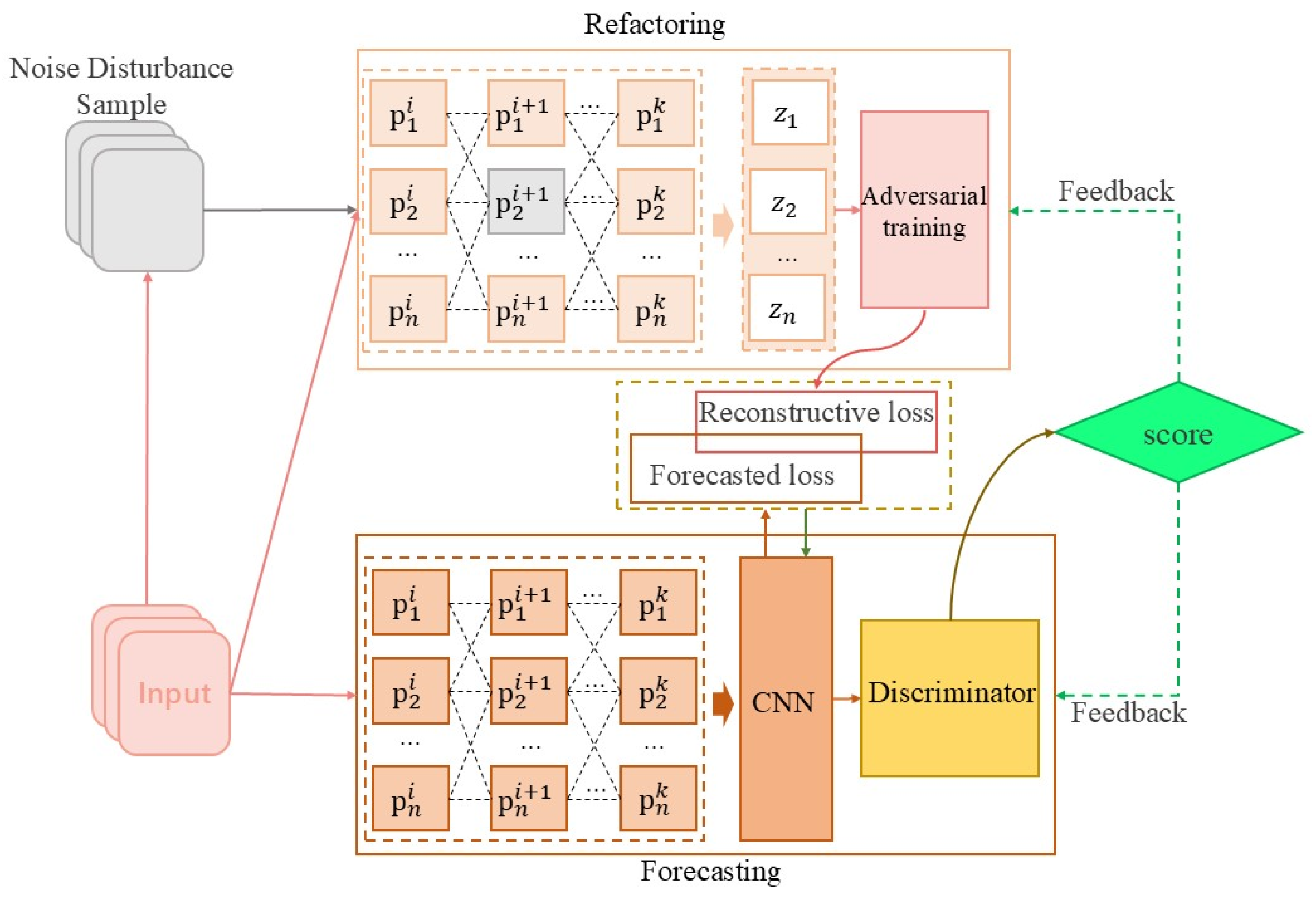
3. PGAT-BiGRU-NRA Framework

This section describes the unsupervised MTSD anomaly detection problem. In response to the fact that existing MTSD processing methods are sensitive to noise and anomalies in the training data, which limits the further improvement of the detection accuracy, a noise adversarial training MTSD processing model compatible with time dependence and spatial correlation for robust anomaly detection of MTSD, as well as a detailed description of the key modules, is provided.

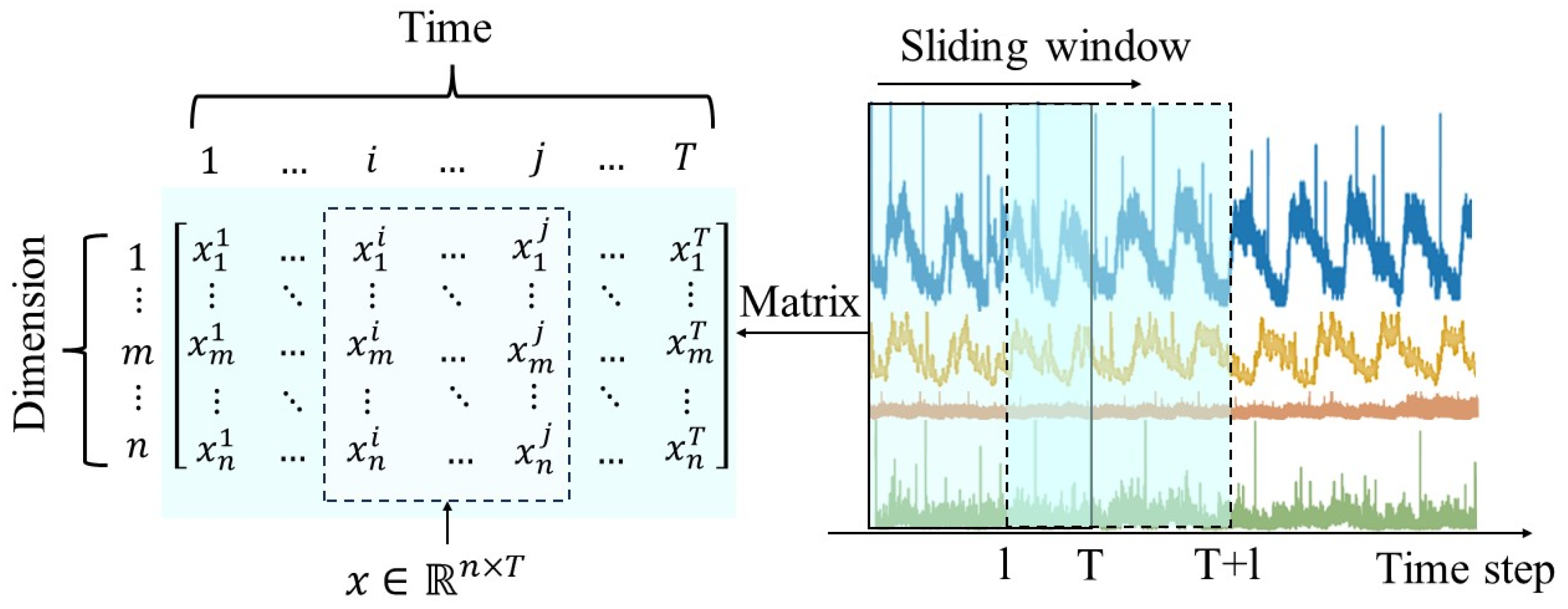
3.1. Description of the Problem

The observed data are defined as Σ = X 1 , X 2 , . . . , X n , where n represents the dimension of the multivariate data. X m is the ordered univariate observed over time in the m dimension, denoted by X m = x m 1 , x m 2 , . . . , x m T , where T indicates the data time step limit within the time window. Σ R n × T in MTSD means data processing aims at fully extracting its temporal and spatial features, calculating the anomaly scores of the test data within a time step, and treating the data corresponding to a time step that exceeds the threshold score as anomalies.
In addition, it is considered that time series acquisition usually contains multiple time nodes, and data between time nodes are captured through a time window using a window size T and a step size l . As shown in Figure 2, the rectangle represents a time window, denoted as a vector-dimensioned time window sliding on the time axis with a step size l .

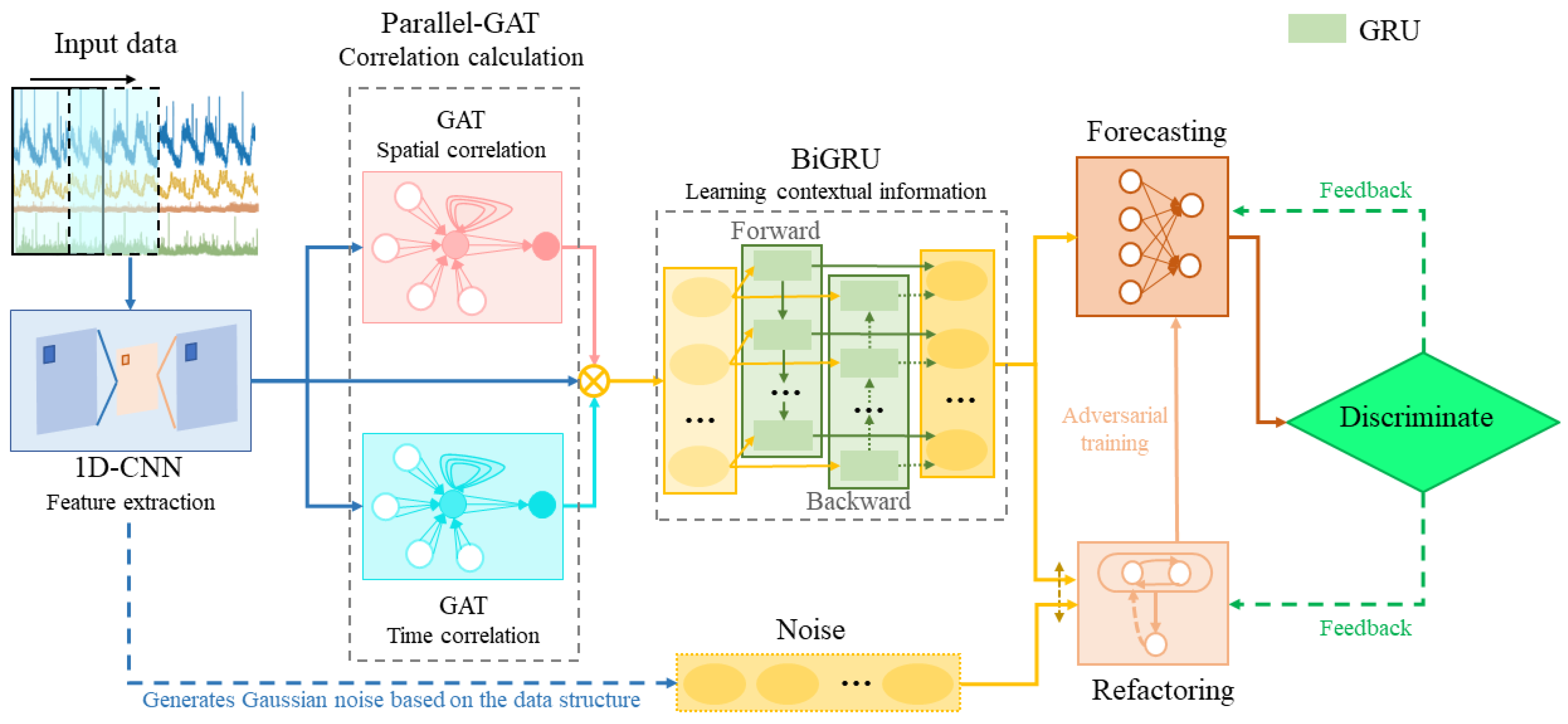
3.2. Overall Framework

The overall framework of the proposed model is shown in Figure 3, in which GATv2 is used to introduce dynamic attention, spatial correlation GAT is used for the extraction of spatial correlation features, and temporal correlation GAT is used for the extraction of time-dependent features of multidimensional time series data. In addition, BiGRU is able to consider both past and future information of temporal data, capturing contextual information through processing inputs in both forward and backward directions. Finally, integrating the advantages of predictive and reconstructive models for anomaly detection tasks, introducing robust joint adversarial optimization, and adding noise countermeasures to the reconstructive model give the whole model a higher robust performance. The implementation details of the architecture will be systematically described in the key technologies in this chapter.
The methodology outlined in the paper comprises the following key steps:
(1)
Data Preprocessing: data preprocessing is performed for MTSD to select normalization methods according to the requirements, and 1D-CNN is applied to extract high-level local features of each time series in the preprocessed data;
(2)
Fusion of Multidimensional Data: parallel GATv2 is used to learn data dependencies from both the temporal dimension and the spatial feature dimension, emphasizing the fusion of multiple features with different weights;
(3)
Learning-Fused Feature Patterns: the BiGRU layer connects the outputs of 1D-CNN and parallel GATv2 to extract contextual information from MTSD and capture time-dependent sequential pattern features;
(4)
Robust Anomaly Detection and Interpretation: VAE reconstructs the model and adds noise countermeasures to improve the robustness of the fully connected network’s joint predictive modeling and obtain the result.

3.3. Key Technologies

3.3.1. Data Preprocessing

The original data are normalized using min-max to make the data of the same size. Local features of the data are identified and extracted using 1D-CNN with a kernel size of 7. min X t r a i n is the minimum value of the training set, and max X t r a i n is the maximum value of the training set.
x i = x i min X t r a i n max X t r a i n min X t r a i n

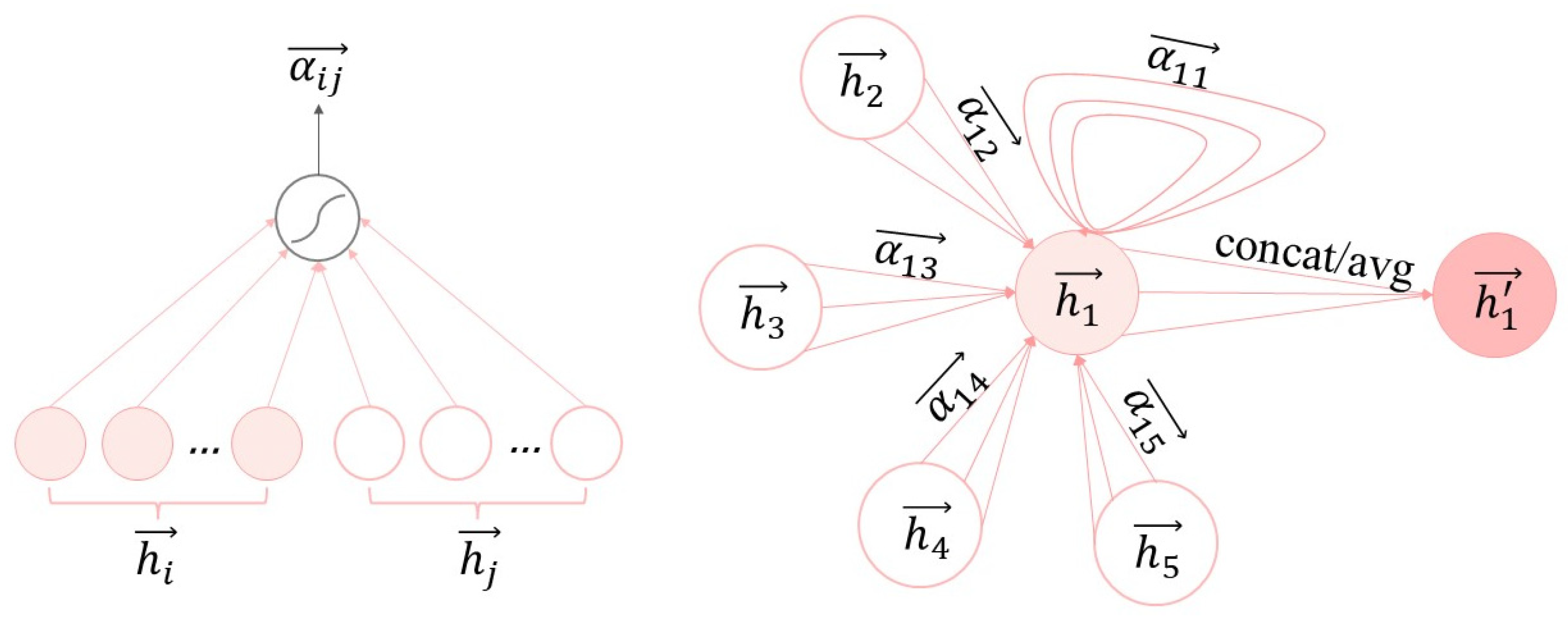
3.3.2. Parallel Improvement of Graph Attention Mechanisms

As shown in Figure 4, the graph structure based on GAT considers the interdependencies between nodes to obtain a new representation of the nodes. Define the input feature vector denoted as h i = h 1 , h 2 , , h N , h i ϵ R F , N represents the number of nodes, and F denotes the feature dimension. The output of each node is calculated through the weighting strategy of GAT as follows:
h i = σ α i , i W h i + j N i α i , i W h j
where h i denotes the output of node i , σ · represents the sigmoid activation function, h j indicates one of the neighboring nodes of node i , and W R F × F means the weight matrix reflecting the relationship between the input and output features.
The degree of association between the nodes is defined as follows:
e i , j = a T L e a k y R e L U W h i | | h j  
where a is the attention learning parameter for the feature dimension, which exp · represents the exponential function of the natural constant e . Therefore, the attention score by mapping nodes is expressed as follows:
α i , j = exp e i , j Σ k N i ˙ i exp e i , k
We use two parallel GATv2 oriented toward spatial and temporal features, respectively, as follows:
The structure of the spatially oriented graph attention layer is designed to detect correlations between multidimensional variables and enable spatial feature extraction without a priori knowledge. MTSD, each node, and each edge are considered as a complete graph, a feature of one dimension, and a correlation between features, respectively, and the inputs are defined as x i = x i t | i 0 , k , t 0 , n , where k denotes the total number of dimensions of multivariate features, and n represents the total number of timestamps in the sliding window, which is used as an input to GAT to extract the spatial features of MTSD.
The time-oriented graph attention layer is structured to capture temporal dependencies in a time series by considering the tiling of a sliding window as a complete graph, each node as a feature vector of the sliding window, and each bar as a correlation between different time windows. Similarly to spatial-oriented GAT, its output is also a k × n vector matrix, and the temporal and spatial features of the parallel GAT output are connected with the local features of the preprocessing output to form an n × 3 k dimensional feature vector, incorporating the comprehensive information of MTSD.

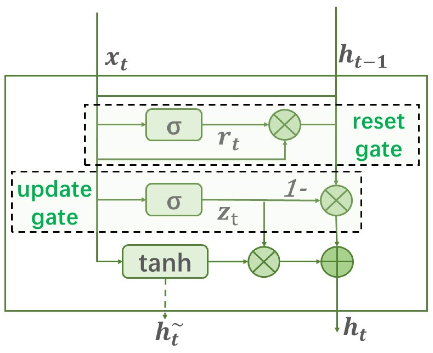
3.3.3. Bi-Directional Gated Recurrent Unit

The anomaly detection of multivariate time series data (MTSD) needs to capture long-term trend anomalies and sudden transient anomalies at the same time. The problem of gradient disappearance and gradient explosion exists in RNN-based data processing tasks. BiGRU can solve this problem and better learn the long-term and short-term temporal dependencies of time series data. The forward GRU captures the long-term cumulative effect of the equipment state, and the reverse GRU verifies the chain reaction of the sudden anomalies. The spatio-temporal features extracted from PGAT are further refined by the contextual modeling of BiGRU, to avoid the loss of features. The GRU unit is shown in Figure 5.
GRU unit contains two key gating mechanisms: the reset gate and the update gate. The reset gate r t = σ W j x t + U j h t 1 captures short-term dependencies, where W j and U j are the weights of the reset gates, and the update gate z t = σ W i x t + U i h t 1 is used to capture long-term dependencies, where W i and U i are the weights of the update gates. The aggregated hidden state of inputs and outputs of the previous layer is h t ~ = t a n h r t U j h t 1 + W h x t . It follows that the native output of the GRU unit is h t = 1 z t · h t 1 + z t h t ~ . In time step t , the forward layer produces the forward hidden layer output to be passed to the next time step for further computation as h t F = t a n h h t 1 , x t . Similarly, the output of the reverse hidden layer at time step t is passed in reverse to time step t 1 as h t B = t a n h h t + 1 , x t . The combination of the forward and reverse layers at each time step is Y t = t a n h h t F , h t B , which fully considers the historical data and future data time characteristics.

3.3.4. Robust Joint Adversarial Optimization

Noise injection into the BiGRU layer followed by the production of reconstructed samples allows the model to learn generalization capabilities against perturbations during training and to dynamically adjust the perturbation magnitude through backpropagation. By superimposing isotropic Gaussian noise, the perturbation direction introduces stochastic deviations from the gradient sign dominance. This noise term compels the model to learn generalization capabilities against neighborhood perturbations during training while preserving the explicit attack directionality of adversarial perturbations to improve robust performance. The perturbation generation formula is expressed as follows:
z = ϵ · s i g n x L f θ x , y + N ( 0 , σ 2 )
The reconstruction model partially learns the distribution pattern of the potential representation of the data. The reconstruction of the sample is to use the game process to set the objective function as follows:
f 1 x = E x r ~ P r · log F x + E z ~ P g · log 1 F ( R z ) f x = m i n θ m a x φ f 1 x  
where P r · represents the distribution of the real data, P g · indicates the low-dimensional spatial distribution of the noise, and θ   a n d   φ denote the reconstruction with the predicted parameters, with the encoder probabilistically selecting between reconstructing the noisy data and the real data to generate the reconstruction of the sample model for robust joint adversarial optimization, as shown in Figure 6.
In the anomaly detection tasks, the proposed model leverages adversarial networks, a reconstruction-based model that captures the data features of the entire time series to add noise for reconstructing the samples, as well as a prediction-based model for predicting future values, improving the robustness of the model through adversarial training of the reconstructed model and the predicted model. The parameters of the two models are updated simultaneously during the training process. The loss function is defined as follows:
L o s s = λ L o s s F o r + 1 λ L o s s R e c
where λ denotes the probabilistic hyperparameters of the reconstruction loss and the prediction loss. The prediction model is partially passed through the fully connected layer after BiGRU and stacked hidden layers for feature extraction. The root mean square error of the final fully connected output layer is defined as the loss function:
L o s s F o r = Σ i ˙ = 1 n ( f F x n + 1 , i f F x ^ n + 1 , i ) 2
where f F x n + 1 , i denotes the value of the prediction model at the next timestamp of the BiGRU output layer for the current input.

3.3.5. Anomaly Detection

The error between the predicted value and the actual value obtained after training the model is defined as an anomaly score using (9). The threshold is based on the 99th percentile of the test set anomaly scores. If the anomaly score exceeds the threshold value, the timestamp is identified as an anomaly. After anomaly detection, the features that cause the timestamp anomaly are determined to speed up the troubleshooting rate. Then, the detected anomalies x t are ranked according to x ^ t i , and the features of the i dimension are finally selected to rank the top k features as the root cause of the anomaly to achieve an explanation of the anomaly.
s c o r e = Σ i = 1 m ( x n + 1 , i x ^ n + 1 , i ) 2
The proposed PGAT-BiGRU-NRA is implemented as Algorithm 1.
A l g o r i t h m   1   P G A T B i G R U N R A   f o r   M T D S   a n o m a l y   d e t e c t i o n
Input :   A   data   matrix   X ,   Queries   labels   matrix   Y ,   the   sliding   window   size   w ,
           the   sliding   step   is   l ,   Iteration   steps   is epochs ;  
Output :   Queries / Classified   labels   y ^ = { y 1 ^ , y 2 ^ , . . . , y t ^ } ;
1.  T = [ 1 , 2 , , t ] ; / / T h e   l e n g t h   o f   t h e   t i m e   s e r i e s ;
2.  N = [ 1 , 2 , , n ] ; / / D i m e n s i o n a l i t y   o f   t i m e   s e r i e s ;
3.  I n i t i a l i z e   t h e   p r o p o s e d   n e t w o r k   m o d e l .
4.  f o r   ( i = 0 ; i < t w ; i + = l )   d o
5.     X 1 1 D C N N ; / / f e a t u r e   e x t r a c t i o n
6.     X 2 T i m e _ f a t u r e _ G A T ( X 1 ) ;
7.     X 3 S p a c e f a t u r e G A T X 1 ;
8.     X 4 B i G R U ( X 1 , X 2 , X 3 ) ;
9.     N o i s e 1 / σ 2 π · e x p X 1 μ 2 / 2 σ 2 ;
10.    R e c o n R e f a c t o r i n g ( X 4 , N o i s e ) ;
11.    F o r e c a s t i n g A d v e r s a r i a l _ t r a i n i n g _ P r e d i c t i o n ( X 4 , R e c o n ) ;
12.  e n d   f o r
13.  f o r   ( e p o c h 1   t o   e p o c h s )   d o
14.    F o r e c a s t i n g m o d e l ( t r a i n _ s e t ) ;
15.    o p t i m i z e r A d a m ( m o d e l . p a r a m e t e r s , l r 0.01 ) ;
16.   i f   ( F o r e c a s t i n g   i s   n o t   f u l l y   d a t a _ l e n g h x i < T )   t h e n  
17.      l o s s   = Σ i ˙ = 1 n ( f F x n + 1 , i f F x ^ n + 1 , i ) 2 ; / / C l a s s i f y   l o s s
18.      U s e   l o s s   b a c k w a r k   a n d   o p t i m i z e r   s t e p   u p d a t i n g   m o d e l ;
19.    e n d   i f
20.   e n d   f o r
21.   x ^ n + 1 , i m o d e l ( t e s t _ s e t ) ;
22.  w h i l e   ( y ^   i s   n o t   f u l l y   l a b e l s )   d o
23.     s c o r e   = Σ i = 1 m ( x n + 1 , i x ^ n + 1 , i ) 2 ;
24.     i f   ( s c o r e > T h r e s h o l d   v a l u e )   t h e n
25.        C l a s s i f y   y i ^ = 1 ;
26.     e n d   i f
27.      i f   ( s c o r e < = T h r e s h o l d   v a l u e )   t h e n
28.        C l a s s i f y   y i ^ = 1 ;
29.     e n d   i f
30.  e n d   w h i l e
31.  r e t u r n   y ^ = y 1 ^ , y 2 ^ , . . . , y t ^ ;

4. Experimental Results and Analysis

4.1. Description of Datasets

Experiments are conducted using three public datasets and datasets collected by laboratory equipment. SMD collects real-time data for a period of 5 weeks on 28 different cloud platform servers, with each machine containing 38 dimensions of data (each dimension is a metric of the machine). SMAP and MSL, respectively, are soil moisture active–passive satellite and Mars science laboratory rover datasets provided by NASA. The experimental equipment is a gearbox platform, and the vibration data of normal and abnormal states are collected and fused as the anomaly detection dataset. To verify the ability of the proposed model to better distinguish between normal fluctuations and anomalies, as well as to assess its migration performance for MTSD, comparative tests are conducted on all the machines in the three datasets, and its efficiency is verified on the laboratory equipment dataset. The statistical characteristics of the dataset are shown in Table 2.

4.2. Experimental Setup

4.2.1. Evaluation Metrics

Precision P , recall R , F 1 scores, and A U C scores are metrics to evaluate the performance of the model against the baseline model. The analysis reveals that most of the state-of-the-art methods regarding A U C scores have been empirically more than 0.97, including the proposed model. Thus, P , R , and F 1 scores are chosen as the evaluation indexes, and they are calculated as follows:
P = T P / T P + F P R = T P / T P + F N F 1 = 2 × P · R / P + R
where T P denotes a true positive example predicted as positive and actually positive, FP indicates a false positive example predicted as positive and actually negative, and F N symbolizes a false negative example predicted as negative and actually positive. To obtain the best F 1 score, it is searched by enumerating all possible thresholds denoted as b e s t F 1 .

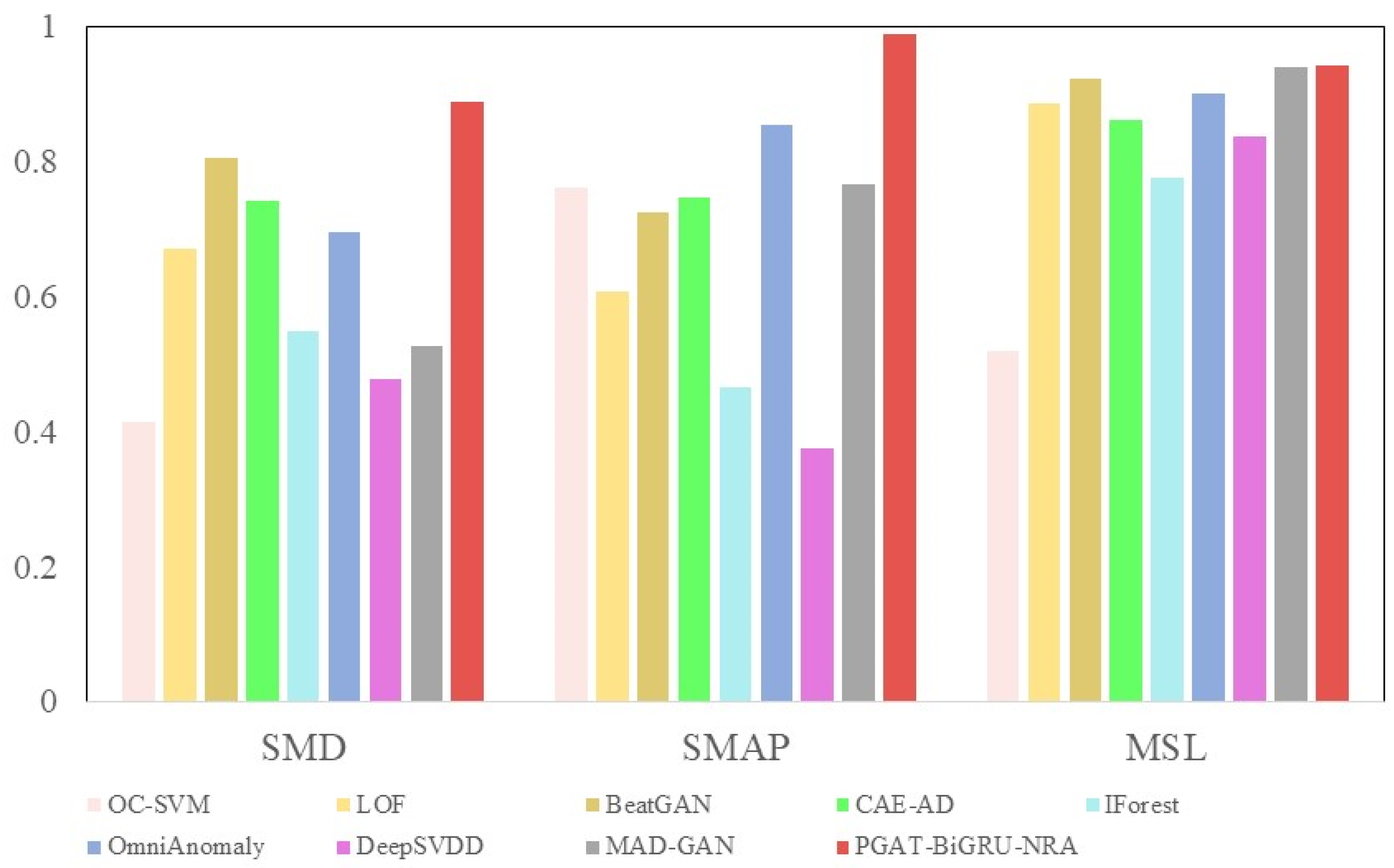
4.2.2. Comparative Methods

In this paper, the proposed method is compared with eight classical baseline models, which are described as follows:
(1)
OC-SVM [33] maps the samples through the kernel function to a higher dimensional space to delineate normal and abnormal boundaries;
(2)
LOF [34] detects anomalies using the local density deviation of the target data relative to the neighborhood;
(3)
BeatGAN [35] is based on an adversarial self-encoder and adds a discriminator to improve the formality of the reconstructed samples;
(4)
CAE-AD [28] enhances data feature representation using a self-encoder combined with contextual information for comparative learning;
(5)
IForest [36] isolates anomalies in the data by modeling the integration of randomly selected features on the division of observations;
(6)
OmniAnomaly [29] considers time-dependent, potentially spatially stochastic modeling to capture complex data distributions;
(7)
DeepSVDD [37] employs a co-training network to learn single-classified target data features for spherical mapping to normal data;
(8)
MAD-GAN [38] is based on recurrent neural networks to capture multivariate temporal distribution features while considering discriminative and generative loss detection anomalies.

4.2.3. Experimental Realization Details

In this paper, PGAT-BiGRU-NRA is implemented with GPU. A 1D-CNN with the same sliding window size w set to 100, a sliding step size l set to 8, and kernel size 7 is used, and the raw training data are divided according to an 8:2 ratio. The amount of neuron data h for BiGRU is set at 150, and the number of layers is set to 1. To train the model, the epoch, batch size, learning rate, and dropout are set to 30, 256, 0.001, and 0.4, respectively, and noise intensity α is set to 0.1. Training is performed with the Adam Optimizer.

4.3. Experimental Results

The performance and explanatory power of PGAT-BiGRU-NRA are tested using three public datasets. The experiment proves that the proposed method outperforms eight typical baseline models. Finally, the proposed model is used for anomaly detection in laboratory equipment and random noise is added to the dataset to prove the effectiveness and robustness of the method.

4.3.1. Analysis of Experimental Results

Table 3 shows that the anomaly detection in the SMD dataset performs poorly in the baseline model. By analyzing the dataset, there are 28 machines in SMD, among which the raw data collected by machines 1–3, 1–8, 2–6, and 3–5 have lower detection accuracy due to the scarcity of anomaly samples and obvious noise interference, which is not enough to train the anomaly detection model and inevitably misclassify normal fluctuations as anomalies. On the other hand, the SMAP dataset has a score of 0.988 because the distribution of anomalies is concentrated, the correlation is stable, and the model is able to effectively capture the characteristic patterns of the data and counteract the noise interference.
The proposed model also shows excellent performance in SMD after adding the noise countermeasure module. Although there is a trade-off in comparing the other baseline models P and R, as shown in Figure 7, the visualization shows that the F1-score of the proposed model outperforms the baseline model in all aspects, which proves that the proposed model has higher robustness and is especially suitable for the complex noise and dynamic anomaly detection needs in industrial scenarios.
The baseline method exhibits different performance across different data. OC-SVM, a lightweight model, delineates anomaly boundaries through kernel function mapping, showing good performance with a small number of anomalous samples but struggles with large-scale datasets and noisy disturbances in the training data. LOF operates based on a clustering model that clusters the target data and performs density estimation to identify anomalies. However, it identifies anomalies when the data points deviate significantly from most of the data. IForest defines anomalies as sparse points that stray from the high-density group, making the anomalous data close to the root while the normal data are far from it by tree modeling. Due to the modeling performance of LOF and IForest, they show superior results on data with low outlier density. DeepSVDD models effectively distinguish anomalies in the high-dimensional space by learning normal category samples, which to some extent can deal with noise in the data with a certain degree of robustness; however, they perform poorly when there is a large difference between the distribution of normal data and anomalous data. BeatGAN, CAE-AD, OmniAnomaly, and MAD-GAN perform relatively well in models based on deep learning, where BeatGAN introduces a discriminator in the encoder model to discriminate the truthfulness of the reconstructed samples and avoid overfitting the model due to reconstruction. CAE-AD introduces comparative learning for nonlinear data representations and constructs clear boundaries for normal data to deal with complex distributions. OmniAnomaly uses a multi-scale attention mechanism to capture anomalies in a time series and emphasizes the importance of global context to better characterize anomaly patterns across the time series. MAD-GAN utilizes a generative adversarial network idea to set up generators and discriminators to learn data distributions through a gaming process, improving the robustness of the model.
In summary, considering the noise and anomalies that can exist in time series data, paying full attention to the spatio-temporal characteristics of the data, and extracting the contextual information to map the overall trend of the data are essential for improving the data processing robustness and the anomaly detection performance in MTSD, which is precisely the reason for the better performance of the proposed model.

4.3.2. Sensitivity Experiments on PGAT-BiGRU-NRA Parameters

Experiments are conducted on the dataset to explore the effect of each parameter on the performance of the model, and the experimental results are displayed in Figure 8. The hyperparameters of the model include the size of the sliding window w , the potential spatial dimensionality h , the negative slope α , and the intensity of the reconstruction noise γ . The model is then used as an example of a model with a sliding window.
Figure 8a shows that in the SMD dataset, the larger the window size, the slightly lower the F1-score. The reason for the analysis may be that the anomalous dependence of the SMD dataset on the short-term contextual features of the time series, where the temporal dependency is prominent in contributing to the results, does not show a significant advantage over the other datasets. Therefore, considering the average results, the default setting of w = 100 is used in the setup, and in the actual application, it is adjusted appropriately considering the periodic characteristics of MTSD.
The latent space dimension h = { 50 ,   100 ,   150 ,   200 ,   250 } retains the multidimensional sample information within the latent space. The larger the h , the richer the information that can be retained for better reconstruction. However, too large h leads to overfitting. Figure 8b depicts that it is not sensitive to h on the SMD dataset and SMAP dataset, and it scores lower on the MSL dataset with h = 50, which may be due to the high data complexity of the MSL dataset and complex correlations between multidimensional data. Thus, h = 150 is chosen as the default setting based on the average.
The negative slope of the graph attention structure α = { 0 , 0.2 , 0.6 , 0.8 , 1 } introduces nonlinear properties that enable the network to learn more complex node relationships. However, a slope that is too large negatively leads to gradient explosion and reduced training stability. Figure 8c illustrates that the reason for lower scores on the MSL dataset when α is 0 may be that the model is not sufficiently extracting the nonlinear properties between the data. However, the model is unstable when α is greater than 0.2. Thus, the average α = 0.2 is selected as the default setting.
The reconstruction noise intensity is set to γ = { 0.01 ,   0.05 , 0.1 , 0.5 , 1 } . When performing adversarial training of noise reconstruction samples, a smaller γ implies less noise feature component learned by the model. Consequently, the processing of test samples with added random noise will misclassify the noise interference as anomalies, leading to a decrease in the model precision. However, a larger γ may lead to learning complex data features, which can decrease the distance between anomalies and anomaly scores of the normal data, resulting in a decrease in the anomaly recognition ability and a reduction in the recall rate. As shown in Figure 8d, γ = 0.1 is defined as the default setting performing best in the results averaged across the datasets.

4.3.3. Ablation Experiment

The validity of the key modules in the PGAT-BiGRU-NRA model is investigated by ablation experiments, and four variant models of the PGAT-BiGRU-NRA model are constructed, including deletion of Time-GAT, deletion of Space-GAT, BiGRU-NRA, PGAT-NRA, and PGAT-BiGRU. Table 4 compares the five variant models with the proposed model, which shows that the proposed model obtains the highest average scores on all three metrics and performs best.
The analysis of the results shows that the performance of the proposed model decreases when the key modules of the proposed model are removed or replaced, and the best results are obtained by the model that incorporates the three proposed main modules. Analyzing the results obtained from the models of the single-graph attention module and no-graph attention module, it can be concluded that MTSD show better results in fusion processing by fully extracting time-dependent features and spatially relevant features and retaining the original characteristics of the data, proving that the parallel graph attention network module is crucial for data fusion processing. It can be concluded from analyzing the results of the replaced BiGRU module that ensuring important information is not lost during the long-term propagation training process is essential. However, the GRU unit can consider the previous data to hide the features. The gating structure of BiGRU can take into account both historical and future data to retain the data features more comprehensively, allowing the module to ensure that the data features are not lost in data processing to improve model performance. The reconstruction module increases the gap between model anomalies and normal data for anomaly scores by reconstructing noisy samples for adversarial training to improve the robust performance of data processing. By analyzing the results of removing the PGAT-BiGRU model and using the model in test samples with added random noise, the lack of model robustness leads to a sharp decrease in performance. The results of the ablation experiments highlight the importance of each module of the proposed method.

4.4. Model Performance Analysis

Experiments are conducted on the dataset collected by the testbed to verify the effectiveness of the proposed model. In order to verify the robust performance of the model, random noise interference, excluding anomalies, was added to the sample data. The precision of the experimental results is 87.6%, which shows that the model achieves better results. To show the results of anomaly detection more intuitively, the anomaly scores and thresholds are visualized with anomaly labels on some of the timestamps of the dataset, as shown in Figure 9. In Figure 9a, the red line indicates the anomaly score, the black line represents the threshold value, the yellow line indicates the anomaly obtained from the model prediction, and the blue line shows the true anomaly value. When the score exceeds the threshold value, it is an anomaly. The values that are wrongly predicted are analyzed in the purple boxes. As shown in Figure 9b, the purple box indicates misjudged anomalies. By analyzing the reason for the error, we see that there are normal fluctuations in the real data in this part, and the sensitivity of the reconstructed part to the fluctuations makes it misjudged as an anomaly. However, from the overall point of view, the model achieves satisfactory results.

5. Conclusions

This paper proposed the PGAT-BiGRU-NRA model, which considered the susceptibility of the existing model to noise and added noise-counteracting reconstruction samples to improve the robust performance of the model. We will conduct experiments on more real datasets to verify the robustness of the model in more complex situations and to realize more complicated tasks, such as anomalous aliasing, to provide more powerful robustness to MTSD processing. However, deep learning models inherently have complex computational degree issues, but the parallel architecture of the proposed model provides a technical basis for distributed deployment at the edge. However, the robustness of the model still needs to be further improved in the face of extreme perturbations. Future work will focus on dynamic noise modeling and adaptive threshold optimization to improve its scalability in smart manufacturing systems.

Author Contributions

Conceptualization, Y.X.; Methodology, Y.X. and J.T.; Writing—Original Draft, Y.X.; Investigation, J.T.; Data Curation, J.T. and R.Z.; Formal Analysis, J.T.; Visualization, R.Z.; Validation, R.Z. and J.W.; Resources, J.W.; Supervision, J.W., J.T. and R.Z. All authors have read and agreed to the published version of the manuscript.

Funding

This research was funded by [The Special Project on Cooperation and Exchange of Shanxi Province Science and Technology] grant number [China No. 202204041101036] and [Guangzhou Science and Technology Plan Project] grant number [China No. 2024B03J1297].

Data Availability Statement

Due to the privacy protection restrictions of the organization, the experimental data is temporarily not supported for public release.

Conflicts of Interest

Author Rui Zhang was employed by Shanxi Information Industry Technology Research Institute Company Ltd. The remaining authors declare that the research was conducted in the absence of any commercial or financial relationships that could be construed as a potential conflict of interest.

Abbreviations

The following abbreviations are used in this manuscript:
MTSDMultivariate time series data
PGATParallel graph attention
NARNoise Reconstruction Adversarial Training

References

  1. Mutawa, A.M. Predicting Intensive Care Unit Admissions in COVID-19 Patients: An AI-Powered Machine Learning Model. Big Data Cogn. Comput. 2025, 9, 13. [Google Scholar] [CrossRef]
  2. Wang, Z.; Shrestha, R.M.; Roman, M.O.; Kalb, V.L. NASA’s Black Marble Multiangle Nighttime Lights Temporal Composites. IEEE Geosci. Remote Sens. Lett. 2022, 19, 2505105. [Google Scholar] [CrossRef]
  3. Lei, Z.; Shi, J.; Luo, Z.; Cheng, M.; Wan, J. Intelligent Manufacturing From the Perspective of Industry 5.0: Application Review and Prospects. IEEE Access 2024, 12, 167436–167451. [Google Scholar] [CrossRef]
  4. Yao, H.; Liu, C.; Zhang, P.; Wu, S.; Jiang, C.; Yu, S. Identification of Encrypted Traffic Through Attention Mechanism Based Long Short Term Memory. IEEE Trans. Big Data 2022, 8, 241–252. [Google Scholar] [CrossRef]
  5. Wan, J.; Li, D.; Tu, Y.; Liu, J.; Zou, C.; Chen, R. A General Test Platform for Cyber Physical Systems: Unmanned Vehicle with Wireless Sensor Network Navigation. In Proceedings of the 2011 International Conference on Computers, Communications, Control and Automation (CCCA 2011), Hokkaido, Japan, 1–2 February 2011; Volume III, pp. 165–168. [Google Scholar]
  6. Blazquez-Garcia, A.; Conde, A.; Mori, U.; Lozano, J.A. A Review on Outlier/Anomaly Detection in Time Series Data. ACM Comput. Surv. 2022, 54, 56. [Google Scholar] [CrossRef]
  7. Santamaria-Bonfil, G.; Reyes-Ballesteros, A.; Gershenson, C. Wind speed forecasting for wind farms: A method based on support vector regression. Renew. Energy 2016, 85, 790–809. [Google Scholar] [CrossRef]
  8. Deng, H.; Runger, G.; Tuv, E.; Vladimir, M. A time series forest for classification and feature extraction. Inf. Sci. 2013, 239, 142–153. [Google Scholar] [CrossRef]
  9. Yan, H.; Tan, J.; Luo, Y.; Wang, S.; Wan, J. Multi-Condition Intelligent Fault Diagnosis Based on Tree-Structured Labels and Hierarchical Multi-Granularity Diagnostic Network. Machines 2024, 12, 891. [Google Scholar] [CrossRef]
  10. Yan, S.; Shao, H.; Xiao, Y.; Zhou, J.; Xu, Y.; Wan, J. Semi-supervised fault diagnosis of machinery using LPS-DGAT under speed fluctuation and extremely low labeled rates. Adv. Eng. Inform. 2022, 53, 101648. [Google Scholar] [CrossRef]
  11. Zhang, Y.; Chen, Y.; Wang, J.; Pan, Z. Unsupervised Deep Anomaly Detection for Multi-Sensor Time-Series Signals. IEEE Trans. Knowl. Data Eng. 2021, 35, 2118–2132. [Google Scholar] [CrossRef]
  12. Tan, J.; Wan, J.; Chen, B.; Safran, M.; AlQahtani, S.A.; Zhang, R. Selective Feature Reinforcement Network for Robust Remote Fault Diagnosis of Wind Turbine Bearing Under Non-Ideal Sensor Data. IEEE Trans. Instrum. Meas. 2024, 73, 3515911. [Google Scholar] [CrossRef]
  13. Gao, J.; Li, P.; Chen, Z.; Zhang, J. A Survey on Deep Learning for Multimodal Data Fusion. Neural Comput. 2020, 32, 829–864. [Google Scholar] [CrossRef] [PubMed]
  14. Wei, Q.; Dobigeon, N.; Tourneret, J.-Y. Fast Fusion of Multi-Band Images Based on Solving a Sylvester Equation. IEEE Trans. Image Process. 2015, 24, 4109–4121. [Google Scholar] [CrossRef]
  15. Liu, Y.; Fan, X.; Lv, C.; Wu, J.; Li, L.; Ding, D. An innovative information fusion method with adaptive Kalman filter for integrated INS/GPS navigation of autonomous vehicles. Mech. Syst. Signal Process. 2018, 100, 605–616. [Google Scholar] [CrossRef]
  16. Wu, J.; Lin, Z.; Zha, H. Essential Tensor Learning for Multi-View Spectral Clustering. IEEE Trans. Image Process. 2019, 28, 5910–5922. [Google Scholar] [CrossRef]
  17. Pan, Y.; Zhang, L.; Li, Z.; Ding, L. Improved Fuzzy Bayesian Network-Based Risk Analysis With Interval-Valued Fuzzy Sets and D–S Evidence Theory. IEEE Trans. Fuzzy Syst. 2020, 28, 2063–2077. [Google Scholar] [CrossRef]
  18. Zhu, C.; Xiao, F.; Cao, Z. A Generalized Renyi Divergence for Multi-Source Information Fusion with its Application in EEG Data Analysis. Inf. Sci. 2022, 605, 225–243. [Google Scholar] [CrossRef]
  19. Fu, H.; Sun, G.; Ren, J.; Zhang, A.; Jia, X. Fusion of PCA and Segmented-PCA Domain Multiscale 2-D-SSA for Effective Spectral-Spatial Feature Extraction and Data Classification in Hyperspectral Imagery. IEEE Trans. Geosci. Remote Sens. 2022, 60, 5500214. [Google Scholar] [CrossRef]
  20. Liang, W.; Xiao, L.; Zhang, K.; Tang, M.; He, D.; Li, K.-C. Data Fusion Approach for Collaborative Anomaly Intrusion Detection in Blockchain-Based Systems. IEEE Internet Things J. 2022, 9, 14741–14751. [Google Scholar] [CrossRef]
  21. Xie, T.; Huang, X.; Choi, S.-K. Intelligent Mechanical Fault Diagnosis Using Multisensor Fusion and Convolution Neural Network. IEEE Trans. Ind. Inform. 2022, 18, 3213–3223. [Google Scholar] [CrossRef]
  22. Baldauf, D.; Desimone, R. Neural Mechanisms of Object-Based Attention. Science 2014, 344, 424–427. [Google Scholar] [CrossRef] [PubMed]
  23. He, C.; Zhang, X.; Song, D.; Shen, Y.; Mao, C.; Wen, H.; Zhu, D.; Cai, L. Mixture of Attention Variants for Modal Fusion in Multi-Modal Sentiment Analysis. Big Data Cogn. Comput. 2024, 8, 14. [Google Scholar] [CrossRef]
  24. Liu, Y.; Yang, S.; Xu, Y.; Miao, C.; Wu, M.; Zhang, J. Contextualized Graph Attention Network for Recommendation With Item Knowledge Graph. IEEE Trans. Knowl. Data Eng. 2023, 35, 181–195. [Google Scholar] [CrossRef]
  25. Ding, C.; Sun, S.; Zhao, J. MST-GAT: A multimodal spatial–temporal graph attention network for time series anomaly detection. Inf. Fusion 2023, 89, 527–536. [Google Scholar] [CrossRef]
  26. Nguyen, H.D.; Tran, K.P.; Thomassey, S.; Hamad, M. Forecasting and Anomaly Detection approaches using LSTM and LSTM Autoencoder techniques with the applications in supply chain management. Int. J. Inf. Manag. 2021, 57, 102282. [Google Scholar] [CrossRef]
  27. Ding, N.; Gao, H.; Bu, H.; Ma, H.; Si, H. Multivariate-Time-Series-Driven Real-time Anomaly Detection Based on Bayesian Network. Sensors 2018, 18, 3367. [Google Scholar] [CrossRef]
  28. Zhou, H.; Yu, K.; Zhang, X.; Wu, G.; Yazidi, A. Contrastive autoencoder for anomaly detection in multivariate time series. Inf. Sci. 2022, 610, 266–280. [Google Scholar] [CrossRef]
  29. Su, Y.; Zhao, Y.; Niu, C.; Liu, R.; Sun, W.; Pei, D. Robust Anomaly Detection for Multivariate Time Series through Stochastic Recurrent Neural Network. In Proceedings of the KDD ’19: The 25th ACM SIGKDD Conference on Knowledge Discovery and Data Mining, Anchorage, AK, USA, 4–8 August 2019; pp. 2828–2837. [Google Scholar] [CrossRef]
  30. Audibert, J.; Michiardi, P.; Guyard, F.; Marti, S.; Zuluaga, M.A. USAD: UnSupervised Anomaly Detection on Multivariate Time Series. In Proceedings of the KDD ’20: The 26th ACM SIGKDD Conference on Knowledge Discovery and Data Mining, Virtual Event. 6–10 July 2020; pp. 3395–3404. [Google Scholar] [CrossRef]
  31. Li, W.; Zhong, X.; Shao, H.; Cai, B.; Yang, X. Multi-mode data augmentation and fault diagnosis of rotating machinery using modified ACGAN designed with new framework. Adv. Eng. Inform. 2022, 52, 101552. [Google Scholar] [CrossRef]
  32. Kong, F.; Li, J.; Jiang, B.; Wang, H.; Song, H. Integrated Generative Model for Industrial Anomaly Detection via Bidirectional LSTM and Attention Mechanism. IEEE Trans. Ind. Inform. 2023, 19, 541–550. [Google Scholar] [CrossRef]
  33. Lyu, S.; Farid, H. Steganalysis using higher-order image statistics. IEEE Trans. Inf. Forensics Secur. 2006, 1, 111–119. [Google Scholar] [CrossRef]
  34. Breunig, M.M.; Kriegel, H.-P.; Ng, R.T.; Sander, J. LOF: Identifying density-based local outliers. In Proceedings of the 2000 ACM SIGMOD International Conference on Management of Data, Dallas, TX, USA, 15–18 May 2020; Volume 29, pp. 93–104. [Google Scholar] [CrossRef]
  35. Bin, Z.; Liu, S.; Hooi, B.; Cheng, X.; Ye, J. BeatGAN: Anomalous Rhythm Detection using Adversarially Generated Time Series. In Proceedings of the Twenty-Eighth International Joint Conference on Artificial Intelligence, Macao, China, 10–16 August 2019; pp. 4433–4439. [Google Scholar]
  36. Liu, F.T.; Ting, K.M.; Zhou, Z.-H. Isolation-Based Anomaly Detection. ACM Trans. Knowl. Discov. Data 2012, 6, 3. [Google Scholar] [CrossRef]
  37. Zhang, Z.; Deng, X. Anomaly detection using improved deep SVDD model with data structure preservation. Pattern Recognit. Lett. 2021, 148, 1–6. [Google Scholar] [CrossRef]
  38. Zhou, Y.; Song, Y.; Qian, M. Unsupervised Anomaly Detection Approach for Multivariate Time Series. In Proceedings of the 2021 IEEE 21st International Conference on Software Quality, Reliability and Security Companion (QRS-C), Hainan, China, 6–10 December 2021; IEEE: New York, NY, USA; pp. 229–235. [Google Scholar] [CrossRef]
Figure 1. Example of MTSD input.
Bdcc 09 00122 g001
Figure 2. MTSD matrix.
Bdcc 09 00122 g002
Figure 3. The overall framework of PGAT-BiGRU-NRA.
Bdcc 09 00122 g003
Figure 4. Structure diagram of GAT.
Bdcc 09 00122 g004
Figure 5. GRU Unit.
Figure 5. GRU Unit.
Bdcc 09 00122 g005
Figure 6. Model for robust joint adversarial optimization.
Bdcc 09 00122 g006
Figure 7. F1-score ranking of all models.
Bdcc 09 00122 g007
Figure 8. Results of parameter sensitivity on the real-world datasets. (a) Sliding window size. (b) Potential spatial dimensions. (c) Figure note the negative slope of the structure. (d) Reconstructed noise intensity. The window size w setting is used to learn the long-term time dependence of MTSD. Experiments are conducted using different window size settings of w = { 25 , 50 , 100 , 150 , 200 } .
Bdcc 09 00122 g008
Figure 9. Visualization of results. (a) Model predictions versus true anomalies. (b) Anomaly scores and prediction results for the error part.
Bdcc 09 00122 g009aBdcc 09 00122 g009b
Table 1. Summary of data fusion methods based on probability, D-S evidence theory, and knowledge.
MethodsModelsImplementationLimitations
ProbabilityBayesian [14]Circulant matrix derivationDifficulty in obtaining a priori probabilities and modeling data when dealing with high-dimensional complex data.
Kalman filtering [15]Attenuation factor perturbs weights
Markov model [16]Singular value decomposition norm
D-S Evidence TheoryD-SBNs [17]Feature fuzzy prior probabilityThe quality function is difficult to define, and the model is not robust enough.
BRDD-S [18]Renyi divergence belief entropy
KnowledgePCASVM [19]Principal component analysisSensitive to noise points and performs poorly in the face of unbalanced datasets.
C-clustering [20]Multiple rounds of clustering
CNN [21]Convert to RGB image
Table 2. Statistical characterization of the datasets.
DatasetsSMDSMAPMSLplatform
Features3825554
Training size23,696135,18358,317500,240
Testing size23,696427,61773,729500,131
Abnormal Rate (%)4.1613.1310.2715.3
Table 3. Performance comparison between the proposed model and the baseline model.
MethodSMDSMAPMSL
PRF1PRF1PRF1
OC-SVM0.4320.3620.4150.4520.2360.7610.5240.4230.520
LOF0.6000.7610.6710.4350.9990.6070.8540.9250.886
BeatGAN0.6940.7120.8060.8320.9260.7240.9030.8530.921
CAE-AD0.6390.6260.7410.8210.8120.7460.7560.6450.861
IForest0.6020.5050.5490.3020.9990.4650.6680.9310.775
OmniAnomaly0.7010.7310.6960.7580.9760.8530.8830.9000.901
DeepSVDD0.7780.3340.4790.4560.2760.3760.9810.7420.837
MAD-GAN0.7310.4090.5270.6080.9990.7650.9350.9440.940
PGAT-BiGRU-NRA0.7640.8830.8870.9800.9970.9880.9050.9820.942
Table 4. Results of the proposed model and its ablated version model.
MethodSMDSMAPMSL
PRF1PRF1PRF1
Delete Time-GAT0.7630.8890.8760.9530.9720.9560.9160.9470.932
Delete Space-GAT0.7590.8720.8650.9830.9760.9610.9090.9530.919
BiGRU-NRA0.6960.7430.7390.9370.9440.9630.8560.9660.908
PGAT-NRA0.7320.8650.8840.9740.9820.9610.8790.9520.914
PGAT-BiGRU0.7020.8140.7930.9360.8920.8290.8830.8940.889
PGAT-BiGRU-NRA0.7640.8830.8870.9800.9970.9880.9050.9820.942
Disclaimer/Publisher’s Note: The statements, opinions and data contained in all publications are solely those of the individual author(s) and contributor(s) and not of MDPI and/or the editor(s). MDPI and/or the editor(s) disclaim responsibility for any injury to people or property resulting from any ideas, methods, instructions or products referred to in the content.

