Article

Enhancing Deep Learning Sustainability by Synchronized Multi Augmentation with Rotations and Multi-Backbone Architectures

by
Nikita Gordienko
*,†,
Yuri Gordienko
and
Sergii Stirenko
Faculty of Informatics and Computer Science, National Technical University of Ukraine “Igor Sikorsky Kyiv Polytechnic Institute”, 03056 Kyiv, Ukraine
*
Author to whom correspondence should be addressed.
These authors contributed equally to this work.
Big Data Cogn. Comput. 2025, 9(5), 115; https://doi.org/10.3390/bdcc9050115
Submission received: 5 February 2025 / Revised: 9 April 2025 / Accepted: 22 April 2025 / Published: 27 April 2025
(This article belongs to the Special Issue Machine Learning and AI Technology for Sustainable Development)

Abstract

:
Deep learning applications for Edge Intelligence (EI) face challenges in achieving high model performance while maintaining computational efficiency, particularly under varying image orientations and perspectives. This study investigates the synergy of multi-backbone (MB) configurations and Synchronized Multi Augmentation (SMA) to address these challenges by leveraging diverse input representations and spatial transformations. SMA employs synchronously augmented input data across MBs during training, thereby improving feature extraction across diverse representations. The outputs provided by these MBs are merged through different fusion strategies: Averaging Fusion with aggregation of predictions and Dense Fusion with integration of features via a fully connected neural network. It aims to increase model accuracy on previously unseen input data and to reduce computational requirements by minimizing neural network size, particularly advantageous for EI systems characterized by the limited computing resources. This study employed MBs with the MobileNetV3 architecture and the CIFAR-10 dataset to investigate the impact of SMA techniques and different fusion strategies on model robustness and performance. SMA techniques were applied to simulate diverse image orientations, and MB architectures were tested with Averaging and Dense fusion strategies to assess their ability to learn diverse feature representations and improve robustness. The experiments revealed that models augmented with SMA outperformed the baseline MobileNetV3 on modified datasets, achieving higher robustness to orientation variations. Models with Averaging fusion exhibited the most stable performance across datasets, while Dense fusion achieved the highest metrics under specific conditions. Results indicate that SMAs incorporating image transformation adjustments, such as rotation, significantly enhance generalization across varying orientation conditions. This approach enables the production of more stable results using the same pretrained weights in real-world applications by configuring Image Signal Processing (ISP) to effectively use SMA. The findings encourage further exploration of SMA techniques in conjunction with diverse camera sensor configurations and ISP settings to optimize real-world deployments.

1. Introduction

Recently, numerous artificial intelligence (AI) approaches, including machine learning (ML) and deep learning (DL) techniques leveraging the traditional neural networks (NNs) and advanced deep neural networks (DNNs), have been effectively used in diverse fields. These techniques have evolved from the foundational contributions [1,2,3,4,5,6] to the state-of-the-art (SOTA) advancements [7,8,9]. The rapid growth of AI models, especially DNNs, has raised concerns about their energy consumption, carbon footprint, and accessibility for resource-constrained applications, particularly in Edge Computing (EC) environments. This highlights the need for lightweight and adaptable architectures capable of maintaining accuracy while reducing resource dependency. SOTA approaches in sustainable AI often focus on model compression, efficient architectures like MobileNetV3 [10], and data-efficient training methods. Techniques such as knowledge distillation, pruning, and quantization have achieved significant progress in reducing model size and computational overhead. However, these methods often require retraining or fine-tuning, adding complexity and resource demands. Another significant challenge is adapting these techniques under real-world conditions to practical needs on EI devices. Due to the limited computational resources of EI devices, it is crucial to carefully balance the performance, model size, and prediction time to align with both hardware requirements and real-world conditions. Furthermore, these methods are predominantly evaluated on benchmark datasets, which may not fully represent the complexities of real-world EI applications, for example, on CIFAR-10, CIFAR-100 [11], and ImageNet [12].
Different challenges and problems can be encountered when using DNN models in different real-world applications. In certain applications, objects consistently maintain a fixed orientation relative to the camera sensor. For instance, in autonomous driving, the vehicle is always oriented perpendicularly to the ground, with surrounding objects generally aligned in the same orientation. Conversely, in fields such as medicine, agriculture, and manufacturing, objects may be captured from unpredictable angles, which can significantly impact model performance. Data Augmentation (DA) techniques are often employed to enhance model robustness in such scenarios; however, these methods typically necessitate larger models with a greater number of parameters. A major challenge in this context is that SOTA AI models are becoming increasingly complex and resource-intensive, which hinders their deployment on EI devices with limited computational resources.
The presented research operates at the intersection of sustainable AI development and efficient deep learning, addressing current challenges in computational resource demands, scalability, and environmental impact. The main aim of this study is to present Synchronized Multi Augmentation (SMA) with Multi-Backbone (MB) architectures. It offers a novel alternative by leveraging diverse input representations, which provide slightly different information about the same object. Simulated representations made by the spatial and orientation data transformations may improve the performance and properties of the model. Some of the properties such as size and inference time are crucial for Edge Intelligence solutions.
Actually, it provides experimental results and comparative analysis of various DNN configurations based on the authors’ recently proposed “multi-backbone (MB) ensembling” and Synchronized Multi-Augmentation (SMA) [13] with different image orientations and spatial transformations. SMA leverages multiple types of augmented input data simultaneously during training across diverse backbone architectures (detailed in the “Materials and Methods” section) to enhance model performance. The outputs from MBs are integrated by the following fusion strategies: (1) “Averaging Fusion” with combination of predictions by averaging and (2) “Dense Fusion” with features merging via a fully connected neural network. The main idea behind the proposed technique is to potentially improve performance (namely, accuracy and prediction time) in EI devices with constrained computational abilities by utilizing multiprocessing. This approach may serve as an alternative to DA for enhancing model generalization. By avoiding the drawbacks associated with large, complex models, it instead employs multiple smaller, similar models that can be deployed on resource-limited processors, facilitating easy scalability. Additionally, this technique enhances processing efficiency by isolating each component from others within the model, thereby enabling parallel processing and reducing overall computation time.

2. Background and Related Work

The studies of MB DNNs have made significant strides, leading to enhanced performance and robustness across a range of applications. By integrating multiple DNN components, this approach strengthens model capabilities and efficiency in handling diverse and complex data. It has proven to be particularly beneficial in areas such as health care applications, autonomous driving, robotics, human–computer interactions, hyperspectral image classification, and anomaly detection. Additionally, various techniques have been introduced to optimize Image Signal Processing (ISP) and leverage different image formats, further improving DNN performance in image classification problems.
The MB technique has emerged as a widely discussed strategy for tackling various tasks. In the medical field, the real-time object detection and tracking abilities for surgical tools are critical for enhancing patient safety and minimizing surgical risks in minimally invasive procedures. Ciaparrone et al. (2020) evaluated SOTA MB Mask R-CNN models, exploring 12 combinations of CNN MBs [14]. Their findings reveal that modern CNN-based architectures are well suited for object detection of surgical tools, with the best configuration achieving 87% average precision (AP). These results highlight the potential of MB configurations for robust object detection and tracking and broader applications in domains.
For example, in the agriculture domain, Tiwari et al. (2024) proposed a novel Hybrid Ensemble CNN (HECNNet) designed for the classification of soybean plant diseases [15]. The HECNNet integrates three powerful backbone networks (ResNeXt, SqueezeNet, and SegNet) each tailored to extract critical features from agricultural imagery through carefully optimized convolutional layers, dropouts, and max-pooling layers. HECNNet operates in three distinct phases: data collection, preprocessing, and classification. A key innovation lies in the ensemble strategy, where prediction scores from the three sub-networks are combined using a weighted sum operation, resulting in a significantly enhanced recognition rate compared to single-network approaches. The proposed method achieves an accuracy of 91.7% and effectively addresses the challenges of soybean disease classification, offering a robust and efficient solution for agricultural disease diagnostics.
In the autonomous driving domain, Ouyang et al. (2020) presented MBBNet, an innovative Multi-BackBone Network with lightweight CNNs tailored for traffic light detection [16]. MBBNet integrates three advanced backbone architectures into a unified framework to enhance detection performance. Testing on real-world datasets highlights the system’s robustness, achieving an accuracy > 94%. This efficient and compact design makes MBBNet a feasible solution for resource-constrained EI systems in autonomous transportation applications.
Ciubotariu and Czibula (2022) introduced a novel Multi-Backbone Multi-Task Network (MBMT-Net) aimed at improving prediction tasks by leveraging multiple specialized feature extractors [17]. Unlike traditional single-task networks with a single backbone optimized for one task, MBMT-Net incorporates parallel pre-trained MBs by merging their outputs and passing them to task-specific heads. The architecture is flexible and can integrate various backbone and head types, significantly expanding its applicability. Experimental results demonstrate that MBMT-Net achieves SOTA performance with a reduced parameter count, surpassing previous semantic segmentation models on the NYUv2 dataset, all while being more efficient and scalable for complex multi-task scenarios.
Shin et al. (2024) have shown the efficacy of using diverse architectures within a single model for anomaly detection on videos [18]. This approach allows them to extract features using pre-trained architectures, including CNN, Contrastive Language-Image Pretraining (CLIP), and Vision Transformer (ViT). By integrating these feature extraction techniques and attention mechanisms, the model delivers exceptional performance in anomaly detection tasks on videos.
For hyperspectral image classification (HSI), Zhang et al. (2024) developed a Data- and Knowledge-driven Deep Multi-view fusion Network (DKDMN) designed to enhance HSI classification [19]. Unlike traditional NN-based approaches that rely solely on data-driven learning, DKDMN integrates HSI data with land-cover distribution. The architecture consists of a Deep Multi-view Network Architecture (DMNA), which combines raw HSI data and knowledge obtained via the Diffusion Model-based Knowledge Learning Framework (DMKLF) to capture complex land-cover distributions and reflect inter-sample relationships. Experimental evaluations on benchmark HSI datasets show that this approach allows it to surpass SOTA methods, achieving significant overall accuracy improvements.
Moreover, individual input sources can be more useful using channel augmentation techniques. Ye et al. (2024) showed a novel channel augmentation technique addressing the challenges of cross-modality matching [20]. Unlike conventional augmentation methods primarily designed for single-modality visible images, this approach focuses on generating color-agnostic images by randomly swapping color channels. This augmentation seamlessly integrates into existing workflows, enhancing robustness against color variations. Experiments on two visible–infrared tasks demonstrate substantial performance improvements, achieving a Rank-1/mAP of 71.48%/68.15% on the SYSU-MM01 dataset, outperforming existing unsupervised methods in accuracy and robustness.
Various augmentation techniques are commonly used for DA, and these same techniques can also be applied to channel augmentation in MB configurations. Cubuk et al. (2019) proposed AutoAugment, a data-driven method to automatically discover optimized data augmentation policies for image classification tasks [21]. Unlike manually designed augmentation methods, AutoAugment employs a search algorithm to identify policies that maximize validation accuracy on target datasets. Each policy consists of multiple sub-policies, where a sub-policy comprises two image processing operations (e.g., rotation, translation, shearing), each applied with specific probabilities and magnitudes. During training, a randomly selected sub-policy is applied to each image in a mini-batch, enhancing diversity. Moreover, the learned augmentation policies demonstrate strong transferability, yielding significant performance gains on diverse datasets. This highlights the potential of AutoAugment to generalize across datasets, offering an automated and effective approach to enhance NN training. However, in this paper, only spatial and orientation transformations were used.
Recent studies have also examined how different image formats impact model prediction outcomes. Most of the current image formats are designed for display purposes rather than specific computer vision (CV) tasks, and they often undergo pre-processing by providers to make them more visually appealing to humans. However, pre-processing may alter or discard critical information needed for CV applications. Different cameras with varying ISPs and image pre-processing procedures can further influence the accuracy of predictions, as these processes may interfere with data which are essential for CV tasks. Recently, Ljungbergh et al. (2023) explored limitations of the traditional ISP operations, which are typically designed to produce visually pleasing images, for downstream CV tasks [22]. They hypothesize that the intermediate representation of such optimized images may be less effective than RAW image representations for tasks like object detection. To address this, the researchers propose a novel approach where ISP operations are optimized directly for the end task by learning their parameters during training. Experimental results on the PASCALRAW dataset validate the hypothesis, showing that RAW image-based models outperform RGB-based counterparts, particularly under challenging conditions such as low light. Xu et al. (2023) explored the potential of RAW sensor data, which inherently retain high dynamic range (HDR) information without requiring extra hardware [23]. A novel dataset with RAW sensor data has been introduced to facilitate DNN-based object detection in HDR scenarios. Leveraging the dataset, researchers have shown that performance of object detection on the RAW sensor dataset significantly outperforms performance of object detection on the standard dynamic range (SDR) dataset under different conditions. Extensive experiments confirmed the superiority of RAW data for object detection and highlighted the importance of texture details and pixel distribution in enhancing DNN-based detector performance.
A promising approach involves transforming RGB images to enhance the ability of models to obtain useful information from the available data. To improve the performance of CV models, particularly in resource-constrained environments, Datta et al. (2023) explored bypassing traditional ISP steps [24]. The effective strategy of inverting the ISP pipeline was proposed by means of converting RGB images into RAW format for training models. This approach enables training on RAW sensor data, which can lead to significant performance gains. In particular, training on RAW images from the COCO dataset has shown to boost test accuracy by 7.1% compared to using standard RGB images. Additionally, to further optimize energy efficiency and bandwidth in ISP-less systems, the integration of analog in-pixel demosaicing with in-pixel CNN computations was proposed, resulting in an 8.1% increase in mean average precision (mAP) when tested on the PASCALRAW dataset.
In addition, ISP can be modified to obtain several representations from the same image. The model CNNs extract features from the group of pixels. But in the case, if a camera orientation is changed, the ability of the model to extract features may be impacted. Hence, the model with MB architecture allows having several input sources with different representations to learn and make orientation-insensitive data.
The evolution and usage of MB DNNs have driven remarkable progress in multiple fields. These DNNs with MB architectures improve feature extraction, enhance overall performance, give robustness, and address resource limitations of EI systems. By integrating multiple backbones, MB architectures enable richer and more diverse data representations, yielding SOTA results in a variety of applications. Recent research has further emphasized optimizing ISP pipelines and image formats to maximize data retention, enhancing the outcomes of CV tasks.
EI hardware, which includes single-board computers, smartphones, autonomous systems, microcontrollers, cameras, and IoT devices with AI capabilities, faces considerable limitations in our previous similar investigations [25,26]:
  • limited computational power of EI devices in comparison to centralized server-based solutions or high-end graphic processing units (GPUs),
  • constrained Random Access Memory (RAM) and general storage capacity limits specific to EI systems,
  • energy-efficient regimes and limited power consumption to extend battery life,
  • real-time processing requirements, as far as often EI applications necessitate low latency for operations in real-time or near-real-time regimes.
That is why, based on these practical experiences [25,26], it is crucial to evaluate the feasibility of developing inherently parallel small DNN models and deploying them on EI devices equipped with sensors with various modalities for real-world applications. It is especially important considering the performance degradation often associated with reducing DL model sizes in various use cases.

3. Materials and Methods

This section outlines the key methodological aspects and experimental components, namely, the dataset, models, and the MB DNN configurations with SMA inputs, as well as the metrics used for performance evaluation.

3.1. Dataset

The CIFAR-10 dataset is a well-established and extensively utilized resource within the domains of CV, ML, and DL for benchmarking and evaluating various algorithms [11] (Figure 1). In this study, CIFAR-10 was selected due to its manageable size (low-resolution images and 10 classes), which allowed for time- and resource-efficient experimentation aimed at demonstrating the feasibility and core principles of the proposed SMA technique. This dataset was specifically prepared to offer a challenging set of diverse images used as a standard benchmark for training and testing the performance of ML/DL models.
With a total of 60,000 color images having a resolution of 32 × 32 pixels, CIFAR-10 is organized into 10 distinct classes, where each class is represented by 6000 images. It contains 50,000 images for training and 10,000 images for testing (Figure 1), providing a robust framework for evaluating model performance across various stages of training and generalization. Given its relatively manageable size and wide range of diverse image content, CIFAR-10 is frequently chosen as a standard benchmark for assessing the performance of image classification algorithms, particularly CNNs.
In the context of DL, CIFAR-10 is used as a popular testbed for exploring new architectures and techniques. Researchers often use this dataset to benchmark the performance of novel models and optimization methods, making it an essential tool for advancing the SOTA in image classification. Additionally, CIFAR-10 is widely used for pre-training models, which can then be fine-tuned on more specific or complex datasets, thus playing a critical role in the field of transfer learning. CIFAR-10 is actually the standard dataset in ML/DL, especially for classification tasks, and used as a benchmark for developing, testing, and validating new ideas and model architectures.

3.2. Baseline Models

Recently, a significant amount of efforts have focused on research and development of the new NN architectures aimed at addressing diverse user demands and requirements across various applications. One such architecture is MobileNet, which becomes a critical achievement in the field of NN efficiency [28]. MobileNet was developed as a response to the need for optimizing DL models with respect to both computational efficiency and speed, especially in resource-constrained environments like EI systems. It represents a substantial evolution of its predecessor, addressing limitations such as training speed and parameter efficiency, and is paving the way for practical applications on devices with constrained computational resources.
A notable variant of this architecture is MobileNetV3, which builds on the basis laid by its predecessors, MobileNetV1 in 2017 [28] and MobileNetV2 in 2018 [29]. MobileNetV3, introduced in 2019, is specifically designed to enhance the efficiency of DL models, particularly for deployment on mobile and EI devices [10]. This version integrates key architectural innovations, which further improve the model’s efficiency by recalibrating channel-wise feature responses. Moreover, MobileNetV3 incorporates automated architecture search strategies, which optimize model configurations through a data-driven approach. These improvements together contribute to the model’s ability to maintain high performance while reducing computational demands.
Among the various configurations of MobileNetV3, MobileNetV3-Small is particularly designed for deployment in environments where computational power is highly constrained, such as smartphones, IoT devices, and EI systems. This variant emphasizes lightweight design elements to achieve optimal performance in terms of both speed and power consumption. As a result, MobileNetV3-Small has found widespread adoption in real-time applications on low-power devices, including mobile applications, embedded systems, and EI computing scenarios. Despite its efficiency, MobileNetV3-Small achieves SOTA accuracy, outperforming many of its predecessors in both accuracy and computational efficiency.
The architectural advancements introduced in MobileNetV3, such as progressive learning and improved scaling, have had a profound impact on the design of subsequent NN models, promoting a shift toward more efficient and scalable DL solutions.

3.3. Multi-Backbone Models

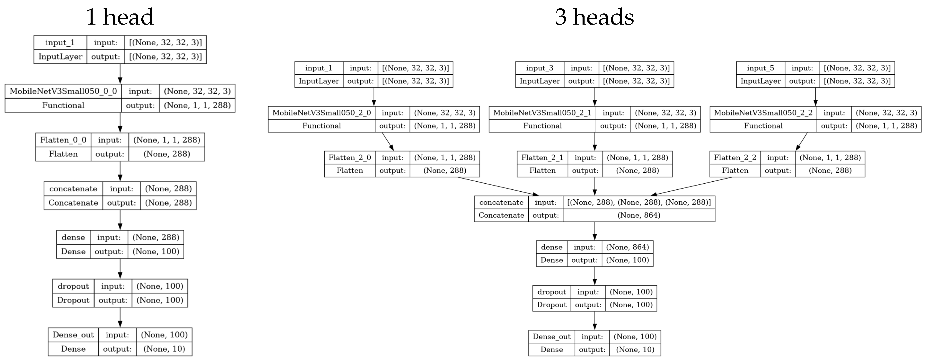
The MB configurations of the MobileNetV3 NN are constructed by merging several MobileNetV3 backbones into a unified NN utilizing a multi-input design. These MB configurations within the MobileNetV3 family typically feature a configuration in which an input layer is sequentially connected to one or more MobileNetV3 backbones. Following the backbone layers, a flattening layer is employed to merge the outputs of the individual backbones, denoted as N, where N { 1 , 3 , 5 } . An averaging layer is then applied to combine the flattened outputs from the various backbones and produce a consolidated output, as illustrated in Figure 2 and Figure 3. This ensemble configuration is designed to improve the ability of the model to process diverse features by aggregating the information from multiple distinct backbone architectures.
The parameter complexity of these models scales with the number of backbones utilized. Specifically, the MobileNetV3 network with a single backbone contains 281,674 parameters, which corresponds to approximately 1.07 MB of model size. When three backbones are used in the ensemble, the MB model’s parameter count increases to 845,022 parameters, or roughly 3.22 MB. Finally, the MB version with five backbones results in a significantly larger model, comprising 1,408,370 parameters and occupying approximately 5.37 MB of storage space.
Another variant of the MB MobileNetV3 architecture employs a different approach to merge the outputs obtained from the individual backbones. Here, the backbone outputs are first flattened, followed by the use of several fully connected layers to combine the information before producing the final output, as demonstrated in Figure 4 and Figure 5. Both of these techniques are tailored to effectively integrate the outputs from multiple backbones, ensuring that the ensemble model leverages the diverse feature representations captured by each individual backbone to enhance overall performance. Here, 3 configurations are evaluated with N backbones, where N { 1 , 3 , 5 } , where the total number of parameters is 308,694 (which corresponds to approximately 1.18 MB), 923,862 (3.52 MB), and 1,539,030 (5.87 MB), respectively.

3.4. Metrics

The performance of the model was evaluated at the training and validation stages of the workflow, conducted using a set of standard metrics. All metrics reported here and in the subsequent sections were computed following the validation process, which included the following:
  • Minimal validation loss: The lowest value of the loss function observed during validation, reflecting the model’s best convergence and generalization capacity.
  • Maximal validation accuracy: The highest classification accuracy achieved on the validation set, representing the best rate of correctly predicted instances.
  • Validation accuracy at minimal loss: The accuracy recorded at the point when the validation loss reached its minimum, helping to assess the model’s predictive performance at optimal convergence.
  • Maximal validation Area Under the Curve (AUC): The highest Area Under the Receiver Operating Characteristic (ROC) Curve, as defined in [30]. This includes both micro and macro AUC variants, which summarize performance across classes in different ways to give a broader perspective on classification quality.
  • Model size: The total number of parameters and the corresponding memory usage (in megabytes), providing a measure of the model’s complexity and storage requirements.

3.5. Workflow

The weights for initialization of DNN models were obtained from a prior training process on the ImageNet dataset [12,31], which is a large-scale collection of labeled images, typically used for training and benchmarking CV algorithms. After the weight initialization, the models were further trained during 30 epochs.
During the training process, the Adam (Adaptive Moment Estimation) optimization algorithm [32] was employed. Adam is a popular optimization algorithm that computes adaptive learning rates for each parameter by considering both the first moment and the second moment of the gradients. The specific hyperparameters used for the Adam optimizer in this study included learning rate 0.001, exponential decay rate for the first moment estimate 0.9, exponential decay rate for the second moment estimate 0.99, and epsilon 10 7 . These hyperparameters are critical for controlling the optimization process and ensuring efficient and stable training of the model. Each of these parameters affects the convergence speed and stability of the learning process.
Experiments were conducted using Kaggle’s GPU runtime environment (NVIDIA P100-PCIE-16GB GPU) with the TensorFlow framework and the Keras library for model implementation. A representative example of the code, including all dependencies and environment setup, is publicly available on the Kaggle platform, as referenced in [33]. Different batch sizes were used during the training experiments, with only slight differences observed in model performance. However, this study did not aim to investigate the impact of batch size on performance. To reduce training time, the largest possible batch size (8192) was selected based on a trade-off between the limitations of Kaggle’s resources and the goal of minimizing training time until model convergence. All random processes were controlled by setting random seeds for both the NumPy and TensorFlow libraries. Data augmentation parameters and model architecture details are explicitly defined in the provided code example.
During model training, each backbone processes the same original image data from the dataset without any augmentations. However, during validation, we employed both the SMA and Test-Time Augmentation (TTA) techniques to enhance model robustness.
The TTA technique [34] was applied to simulate different camera orientations, effectively modeling the object from previously unobserved angles. By augmenting each validation image with rotated versions, TTA creates a scenario where the model must generalize across multiple unexpected perspectives. It helps to evaluate the robustness property of the model to various orientations.
The SMA technique enables us to simultaneously feed the NN with the original image along with various synchronized modifications (data augmentations). This approach allows us to train the MB NN and analyze the impact of each type of DA on the performance of the model in a controlled manner. Through SMA, we emulate having multiple input sources of the same modality but configured differently; these are processed by separate backbones within a single NN model, effectively simulating a fusion of multiple perspectives within the model’s architecture.
The following important aspects should be emphasized as to the role and effect of TTA and SMA. TTA typically applies various augmentations to the input image during inference only, generating multiple predictions which are then averaged or ensembled externally to produce a final result. It operates outside the model, treating the neural network as a black box and requiring no architectural changes. In contrast, SMA is an integrated architectural approach applied during both training and validation. Rather than processing augmentations sequentially and externally, SMA feeds multiple synchronized augmented views of the same input simultaneously into the network, with each view processed by a separate backbone branch. These branches are part of a unified architecture, and their outputs are fused within the model. This strategy enables the model to learn internalized representations that account for variability in sensor settings, preprocessing configurations, or perspectives—emulating a multi-sensor or multi-configuration system. Thus, SMA is not simply a test-time enhancement; it is a training and inference paradigm that encourages the network to develop robustness and generalization across synchronized but diverse views, making it fundamentally different from TTA in both implementation and theoretical grounding.
Moreover, the combination of SMA and TTA emulates a system that operates with several input sources, each capturing images from different, potentially unexpected orientations. This combined approach enhances the ability of the model to handle complex, multiview data in real-world applications where viewpoint variations are common. It will help us to evaluate the impact of the SMA technique on the robustness property.
To implement these augmentations, we utilized the Python Imaging Library (PIL) [35] to create modified inputs for additional channels during both TTA and SMA. Specifically, we applied PIL’s “rotate” method to achieve controlled rotations. This function rotates images counterclockwise by a specified degree around the image’s center, providing a consistent means to simulate multiple orientations across the model’s backbones.
This study utilized four distinct validation datasets, as outlined below:
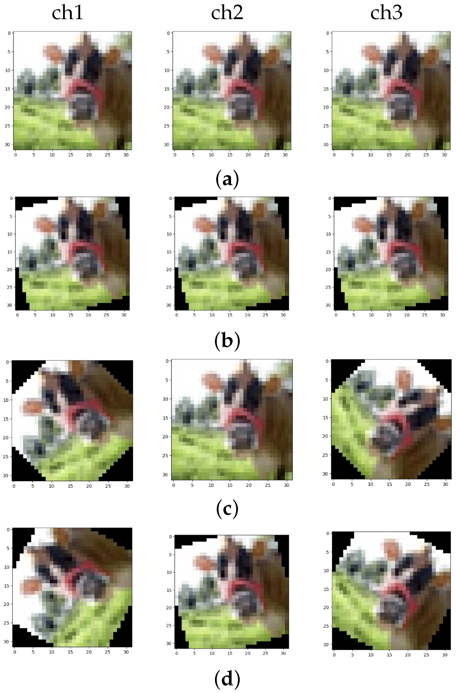
  • “original” (Figure 6a and Figure 7a): Each channel receives the original unmodified image.
  • “simulation” (Figure 6b and Figure 7b): Each channel receives the same original image, modified similarly by being rotated at the same random angle α r . This configuration simulates image capture with identical random camera orientations across all channels. All images are rotated counterclockwise around the center by a random angle between −90 and 90 degrees.
  • “SMA” (Figure 6c and Figure 7c): Each k-th channel in the configuration with N c h channels receives a version of the original image that has been rotated by the angle α k N c h :
    α k N c h = 0 , if N c h = 1 , 45 + 90 k 1 N c h 1 , if N c h > 1 .
    where the channel numbers k are in the range of k { 1 , , N c h } and rotations are in the range of angles α { 45 , , 45 } degrees.
This configuration simulates simultaneous image capture by multiple cameras oriented differently to capture the same scene.
For the single-backbone model ( N c h = 1 ), this configuration is identical to the “Original” setting and α k = 1 N c h = 1 = 0 .
For the 3- and 5-backbone models, each channel receives an augmented version of the image, rotated within a range of −45 to 45 degrees from the original.
Specifically, for the 3-backbone model ( N c h = 3 ), channel 1 ( k = 1 ) receives the image rotated by the angle α k = 1 N c h = 3 = 45 degrees, channel 2 ( k = 2 )—the original image because α k = 2 N c h = 3 = 0 degrees, and channel 3 ( k = 3 )—the image rotated by the angle α k = 3 N c h = 3 = 45 degrees.
Also, for the 5-backbone model ( N c h = 5 ), channel 1 ( k = 1 ) receives the image rotated by the angle α k = 1 N c h = 5 = 45 degrees, channel 2 ( k = 2 )—the image rotated by the angle α k = 2 N c h = 5 = 22.5 degrees, channel 3 ( k = 3 )—the original image because α k = 3 N c h = 5 = 0 degrees, channel 4 ( k = 4 )—the image rotated by the angle α k = 4 N c h = 5 = 22.5 degrees, and channel 5 ( k = 5 )—the image rotated by the angle α k = 4 N c h = 5 = 45 degrees.
  • “SMA + simulation” (Figure 6d and Figure 7d): Each channel receives a combination of “SMA” and “simulation” rotations; namely, each k-th channel in the configuration with N c h channels receives a version of the original image that has been rotated by the angle α k N c h (1) (“SMA”) and the same random angle α r is added (“simulation”), with the result being the range of angles { α 1 N c h + α r , , α k N c h + α r } .
This configuration simulates simultaneous image capture with different camera orientations while introducing a random rotation to the entire scene. One channel receives the original image rotated randomly between −90 and 90 degrees counterclockwise, while other channels receive augmented copies of this rotated image.
For the single-backbone model, this configuration is equivalent to “Simulation”.
For the 3-backbone model ( N c h = 3 ), channel 1 ( k = 1 ) receives the image rotated by the angle α k = 1 N c h = 3 = 45 + α r degrees, channel 2 ( k = 2 )—the original image rotated by the angle α r degrees, and channel 3 ( k = 3 )—the image rotated by the angle α k = 3 N c h = 3 = 45 + α r degrees.
In a similar way, for the 5-backbone model ( N c h = 5 ), channel 1 ( k = 1 ) receives the image rotated by the angle α k = 1 N c h = 5 = 45 + α r degrees, channel 2 ( k = 2 )—the image rotated by the angle α k = 2 N c h = 5 = 22.5 + α r degrees, channel 3 ( k = 3 )—the image rotated by the angle + α r degrees, channel 4 ( k = 4 )—the image rotated by the angle α k = 4 N c h = 5 = 22.5 + α r degrees, and channel 5 ( k = 5 )—the image rotated by the angle α k = 4 N c h = 5 = 45 + α r degrees.
The entire experimental procedure incorporated cross-validation, a robust technique used to estimate generalizability and performance of the model. In this case, the training part of the CIFAR-10 dataset was partitioned into 6 subsets, commonly referred to as folds. Cross-validation involves training the model several times and each time using a different subset of the data for validation, while the remaining subsets are used for training. This method helps to ensure that the model is not overfitting to any particular portion of the data, thereby providing a more reliable estimate of performance of the model on previously unseen data.
In our study, we adopted a K-Fold cross-validation strategy with K = 6, as described in the publicly available notebook [33]. The dataset was split using both KFold and StratifiedKFold methods from the scikit-learn library [36]. Both methods yielded similar results, and the outcomes presented here are based on the KFold partitioning and the typical example includes the implementation of KFold [33].
Each of the six folds was used as a validation subset once, while the remaining five folds were used to train the model. The validation set, which is distinct from the training data and serves to evaluate model performance, was used to measure various validation metrics for each fold. These metrics provide quantitative measurements of how well the model is performing in tasks such as classification, including accuracy, precision, recall, and others.
The mean and standard deviation of these validation metrics were then computed across all folds. The mean is a statistical measure representing the average value of the metrics across the different folds, while the standard deviation measures the variability or spread of the metrics around the mean. By calculating these values, we assess the statistical reliability of the results, where a low standard deviation indicates consistent model performance, and a high standard deviation suggests variability in model performance across different folds.

4. Results

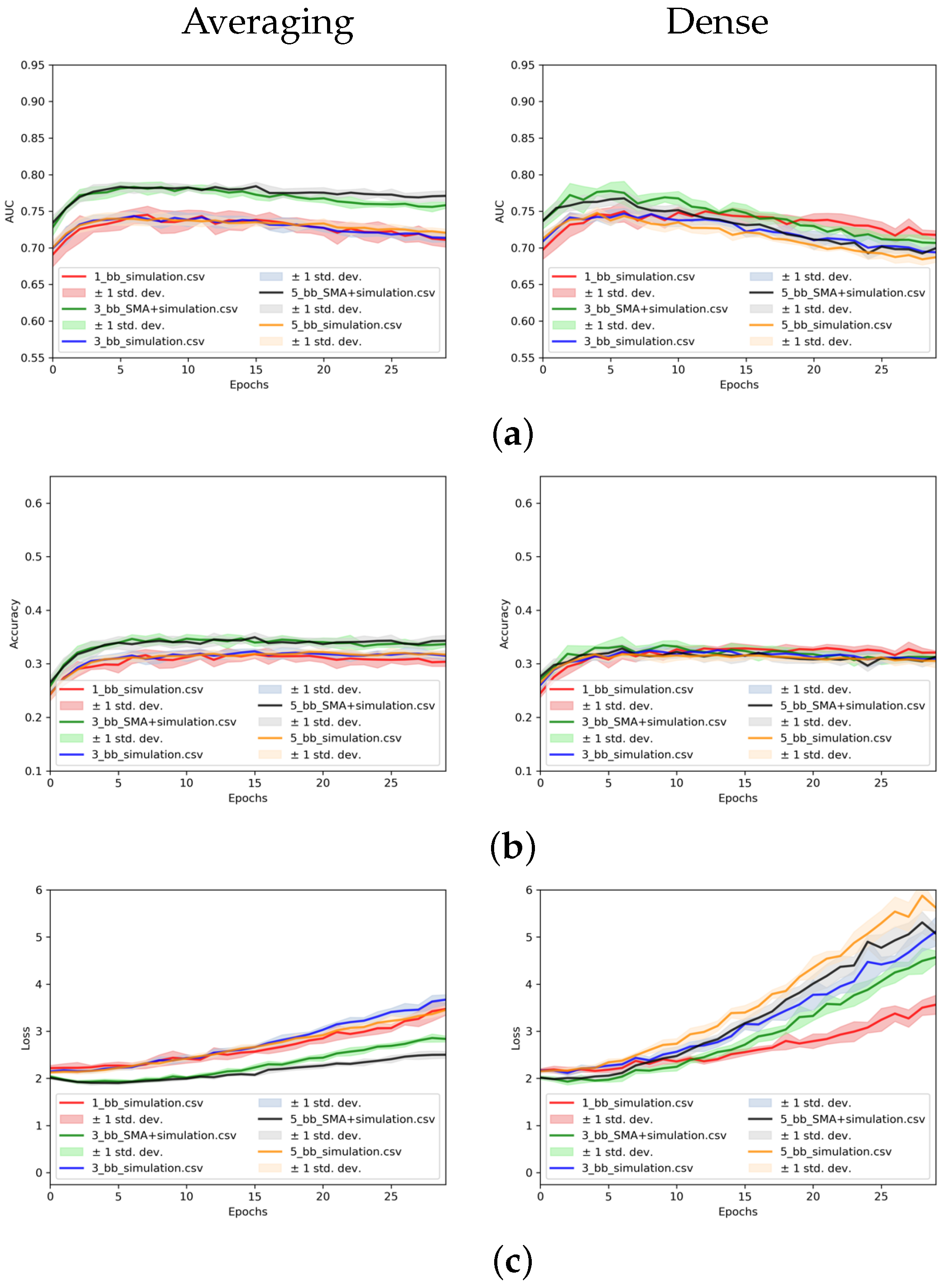
Below, the single-backbone model is considered as a baseline since it employs the original architecture. The histories of some validation metrics (here, accuracy, loss, and AUC) observed with MB models using the SMA technique are presented in Figure 8 for validation on the “SMA” dataset and in Figure 9 for validation on the “simulation” and “SMA + simulation” datasets.
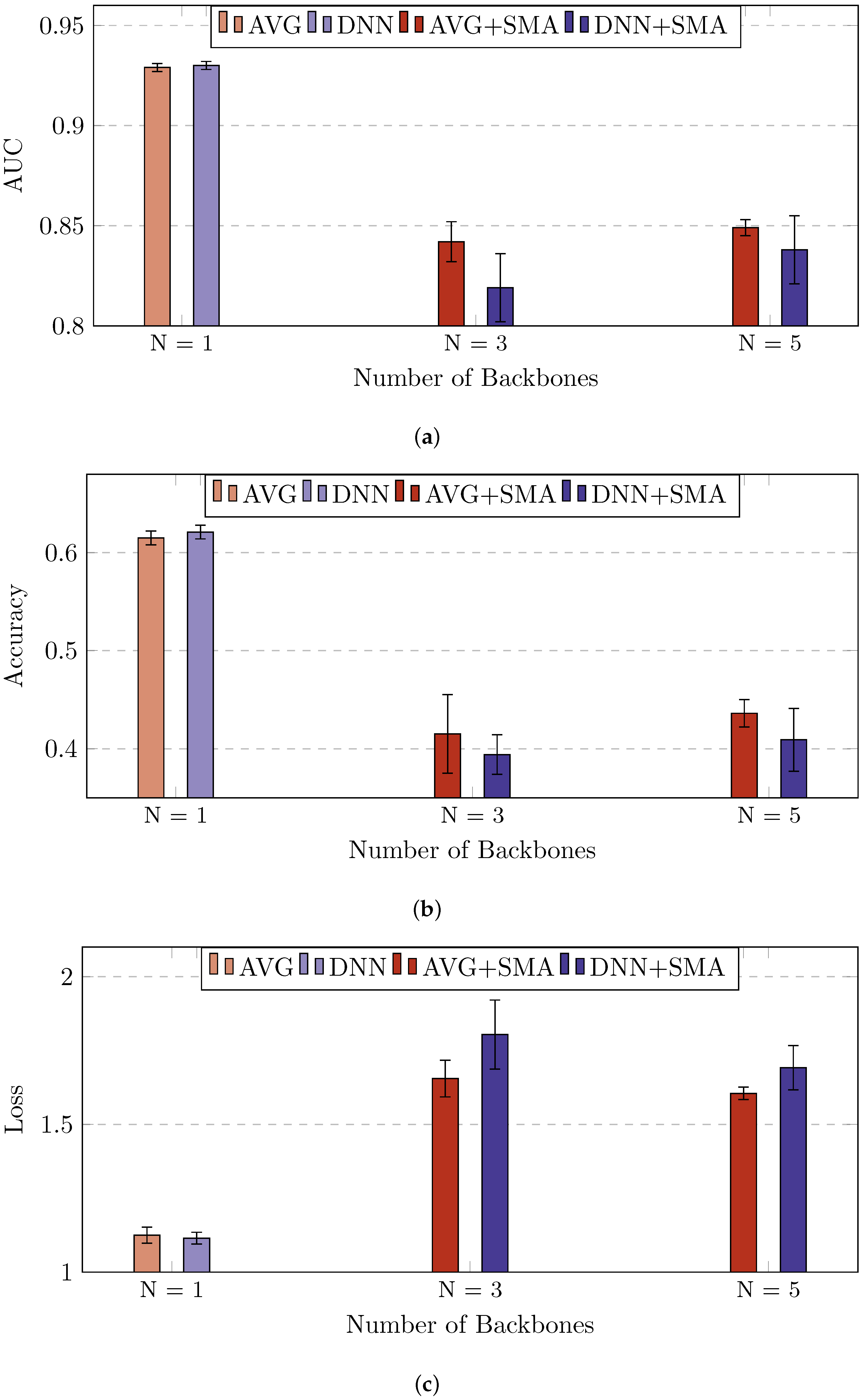
All models were trained on the original dataset, but the validation metrics were analyzed, and their best values (minimum for Loss, maximum for AUC and Accuracy) and metrics values (mean ± standard deviations) were summarized in Table 1 and Table 2 for the “SMA” validation dataset and various fusion methods (Averaging and Dense). For a better visual comparison of the results in Table 1 and Table 2, they are visualized in the bar plots (Figure 9 and Figure 10).

4.1. Validation on the “SMA” Dataset

The mean and standard deviation values of the validation metrics for models trained on an original dataset and evaluated on the “SMA” dataset are shown in Figure 8. The models were trained with varying numbers of backbones N { 1 , 3 , 5 } .
From the technical point of view, the extended history plots (Figure 8 and Figure 9) clearly demonstrate a degradation in validation accuracy and AUC, even as the training loss continues to decrease. These trends are indicative of the model starting to memorize the training data rather than generalizing well to unseen samples, i.e., an established signal of overfitting. Moreover, the corresponding loss plots exhibit pronounced global minimums, which support our interpretation that the model continues to optimize the training objective while generalization performance plateaus or deteriorates.
The plots (Figure 8) show the evolution of three metrics over epochs and their comparison shows that all metrics generally improve with more epochs for all backbone numbers.
For the Averaging fusion (Figure 8, left), in terms of AUC, loss, and accuracy, the multi-backbone models with three and five backbones performed worse than the single-backbone model. However, the model with five backbones outperformed the three-backbone model by a margin exceeding the standard deviation.
For the Dense fusion (Figure 8, right), the performance of multi-backbone models decreased with the increase of the number of epochs, differing from the single-backbone model. This suggests that multi-backbone models with the Dense fusion tend toward overtraining over time. In terms of AUC, loss, and accuracy, both three- and five-backbone models underperformed relative to the single-backbone model, with the five-backbone model failing to outperform the three-backbone model beyond the standard deviation. These findings indicate that Dense fusion is less stable and more susceptible to overfitting. For N > 1 , the Dense fusion models much faster reach the overtraining stage in comparison with the Averaging fusion. The Averaging fusion demonstrates a more stable plateau for all metrics in comparison to the Dense fusion, where overfitting is observed after five epochs already.
The best (minimum for Loss, maximum for AUC and Accuracy) metrics values (mean ± standard deviations) for the models trained on the original dataset and validated on “SMA” validation dataset and for various fusion methods (Averaging and Dense) are shown in Table 1. In general, the baseline single-backbone model outperformed multi-backbone models for both Averaging and Dense fusions on the “SMA” validation dataset.
For a better visual comparison of the results in Table 1, they are visualized in the bar plots (Figure 10), where degradation of performance for MB models was quite pronounced and beyond the standard deviation limits. It should be noted that, actually, the AVG and DNN regimes in Figure 10 (and the other bar plots below) for the single-backbone models are the same because fusion is not used in the single-backbone models. For AVG, an Averaging layer with no effect is added. For DNN, the single Dense layer is added additionally to the state-of-the-art model.
For the “SMA” dataset, the validation AUC history indicates that the Averaging fusion shows the lower standard deviation values compared to the Dense fusion, suggesting greater stability. During validation without simulating varied angle conditions, both Averaging and Dense fusions achieve similar performance. However, the Averaging fusion appears to be less prone to overfitting, maintaining consistent results throughout the training process. In contrast, the Dense fusion reaches peak performance more rapidly but suffers a subsequent decrease in accuracy. This decline means that while the Dense fusion can achieve high initial results, the Averaging fusion provides a more reliable, steady performance across validation rounds.

4.2. Validation on the “Simulation” and “SMA + Simulation” Datasets

The mean and standard deviation values of validation metrics for the models trained on the original dataset and evaluated on the “simulation” and “SMA + simulation” datasets are shown in Figure 9. The models were trained with varying numbers of backbones N { 1 , 3 , 5 } . The plots (Figure 9) show the evolution of three metrics over epochs, and their comparison shows that all metrics generally improve with more epochs for all backbone numbers.
For the Averaging fusion, MB models maintained consistent performance resembling the behavior of the single-backbone model. MB models with three and five backbones on the “SMA + simulation” validation dataset demonstrated better AUC, loss, and accuracy metrics than both the single-backbone model and MB models on the “simulation” validation dataset. Additionally, the MB model with five backbones produced more stable results throughout training, with AUC surpassing that of the MB model with three backbones by a margin greater than the standard deviation in the final epochs. This suggests that the MB model with five backbones is less prone to overtraining.
For the Dense fusion, MB models experienced performance declines with increased epochs, diverging from the single-backbone model’s behavior. After all epochs, the single-backbone model exhibited higher metrics than any MB models using the Dense fusion, suggesting these configurations are prone to overtraining over time. The highest metrics observed for the models with three and five backbones occurred in the early epochs, with AUC values approaching the best levels observed during the Averaging fusion.
The best (minimum for Loss, maximum for AUC and Accuracy) metrics values (mean ± standard deviations) for the models trained on the original dataset and validated on the “SMA” validation dataset and for various fusion methods (Averaging and Dense) are shown in Table 1. In general, the baseline single-backbone model outperformed MB models for both Averaging and Dense fusions on the “SMA” validation dataset.
For the “simulation + SMA” and “simulation” datasets, a similar trend is observed as on the “SMA” dataset when comparing Dense and Averaging fusion. Dense fusion achieves optimal results early on, but with continued training, there is a significant performance drop, ultimately causing the model to underperform relative to a single-backbone model. On the other hand, Averaging fusion remains consistent across all 30 epochs, with the model’s performance stabilizing over time. Notably, in later epochs, the five-backbone Averaging model outperforms the three-backbone version, demonstrating that additional backbones can help maintain performance stability and reduce the tendency toward overtraining.
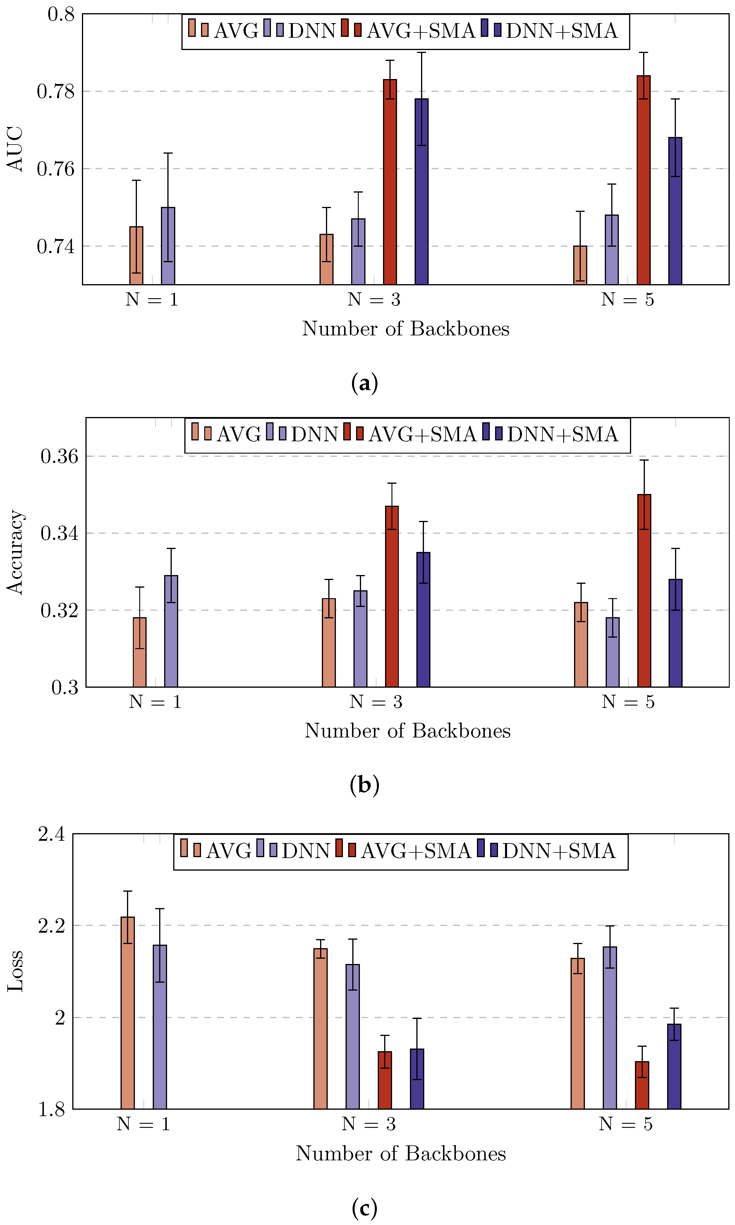
For a better visual comparison of the results in Table 2, they are visualized in the bar plots (Figure 11).

5. Discussion

The experimental results for MB configurations on the basis of the MobileNetV3Small DNN architecture offer valuable insights as to the impact of SMA, particularly for the possible real-world applications in EI setups.
The proposed architectural modifications provide several advantages. By utilizing multiple parallel processes or processors, this approach can enhance query performance speed (QPS) and optimize inference time. Furthermore, it enables model scalability to suit varying user requirements, achieving an effective balance between accuracy, inference time, and hardware constraints.
The results show that the single-backbone model achieves the highest AUC (0.93) when validated on the original dataset, but its performance significantly declines to an AUC of 0.75 when faced with previously unseen data, such as simulated rotations. However, when the SMA technique is applied by adding additional backbones with identical structures, the model demonstrates improved robustness to such unexpected conditions. Specifically, the model with SMA gives an AUC of 0.85 on the “SMA” dataset and 0.78 on the “simulation + SMA” data, illustrating that SMA improves the model to handle varying orientations and positional shifts more effectively. In comparison, the single backbone model achieved only 0.75 on “simulation” data.
This improvement suggests that the SMA technique, rather than merely adding parameters, introduces beneficial diversity to the data each backbone receives. Interestingly, when additional backbones are incorporated without SMA, the model performs similarly to the single-backbone model, despite the increased parameter count. This outcome highlights that it is not just the size of the DNN (characterized by the number of parameters and storage size) but the diversity in input data through SMA that drives the performance gains. Other types of data transformation may yield additional performance gains in the various user cases.
Using SMA means that during validation and its final usage, each backbone processes slightly altered representations of the same object, leading to greater adaptability without further fine-tuning. This reconfiguration of input channels allows for additional data perspectives without modifying model weights. Consequently, SMA can enhance the model’s performance on diverse applications by training solely on the original dataset, making it a practical solution for scenarios requiring robust performance against varied orientations or camera angles.
The reasoning behind the proposed approach is grounded in the observation that a DNN model’s capacity to “learn” new information is inherently constrained by its number of parameters. While a larger parameter count allows the DNN model to learn a greater variety of data representations, it also increases the time and data required for training. Moreover, larger models demand greater computational resources, resulting in higher power consumption and longer processing times. In contrast, the proposed approach leverages alternative data representations at the application level. Instead of augmenting data during training, multiple inputs are utilized, allowing the model to benefit from the hardware and software architecture. This approach enables the generation of different representations of the same input data, which are then processed as distinct inputs in a DNN model. The hypothesis is that this technique will yield more robust model outcomes against modifications not accounted for during training. This shift enables a transition from the traditional paradigm of enlarging the model to learn new representations. The new proposed paradigm is utilizing hardware and Image Signal Processing (ISP) optimizations to preprocess the input data and benefit the model performance.
This technique addresses a key challenge in deploying DNNs in real-world applications. Model training demands substantial computational resources, time, and additional data for optimization and fine-tuning, with dataset creation itself being highly resource-intensive. However, the proposed approach improves model performance while retaining the original model weights. This suggests that, in certain cases, the challenges associated with fine-tuning can be mitigated through the SMA technique at the application level. By preprocessing input data, applications can achieve high accuracy without additional training or fine-tuning. Leveraging the hardware and software architecture for input data preprocessing can further enhance efficiency, potentially outperforming larger models trained on extensive datasets.
Averaging fusion has shown to be more stable than Dense fusion in multi-backbone (MB) models, providing balanced results across backbones and helping to avoid local minima. The Averaging fusion technique stabilizes outcomes by balancing contributions from each backbone, which is particularly beneficial when variations or noise are present in the data. In contrast, Dense fusion can achieve almost the same performance on the dataset by assigning specific weights to the backbones, allowing more flexibility in how each backbone influences the final output. Dense fusion may be better suited to tasks with low data variability, where robustness to numerous data variations is less critical, while Averaging fusion is ideal for applications where data are subject to frequent, unpredictable changes. Averaging fusion enhances robustness by reducing the impact of any one backbone’s false positives, especially if one backbone outputs high-confidence yet inaccurate predictions.
In the current study, we intentionally focused on Averaging and Dense fusion as fundamental baselines to validate the core idea of the SMA technique and to demonstrate its effectiveness under different but representative conditions. These strategies were selected due to their simplicity and wide applicability, making them a solid starting point for understanding how SMA interacts with different fusion mechanisms. That is why exploring more advanced approaches (like weighted averaging, learned fusion parameters, attention-based mechanisms, etc.) is a quite promising extension of the current research. These methods could reveal further ideas in how SMA behaves across various configurations and tasks, and we consider this a valuable direction for future work to enhance the flexibility and generalizability of the MB architecture.
In general, MB architectures within (DNNs) hold promise for meeting the constraints typical in EI systems, like limited memory, power consumption, processing power, and the real-world requirements for real-time response. The MB model architecture is particularly advantageous in these environments because it reuses the same configuration across backbones. This setup potentially allows for partial weight sharing, as each backbone is an identical copy of the original network. By initializing configurations with multiple backbone counts, MB architectures can scale efficiently based on computational requirements, reducing memory storage demands for model deployment.
By employing multiple lightweight backbones, MB architectures in combination with SMA can distribute computational load while maintaining the necessary accuracy and making MB with SMA architectures well suited to resource-constrained EI devices. Low-latency processing, optimized memory use, and SMA’s capacity to handle different object orientations and camera perspectives contribute to reliable performance in real-time applications. Additionally, SMA provides increased robustness to varying camera orientations without additional training, enhancing model performance on original datasets alone.
One of the central challenges in Edge Computing is managing available resources with limited computing and storage abilities. To address this, instead of performing SMA image transformations on the CPU, multiple camera sensors positioned at different angles or ISPs can generate varied representations of the same scene. In many real-world applications, object orientation relative to the camera cannot be controlled. With SMA, these challenges can be mitigated without needing additional datasets or retraining. Leveraging ISP settings to modify image processing could allow edge devices to handle more data variation, offsetting the need for large models and improving efficiency.
A fully parallel structure in MB architectures also benefits inference time, as each backbone can process data independently until the final fusion stage. This parallel processing minimizes resource contention, which is vital for EI scenarios where rapid response times are required. In this way, SMA and MB approaches can be fine-tuned to meet stringent edge hardware demands, driving future advancements in edge AI. However, further evaluation of the specific impacts of different SMA techniques on robustness and performance remains an area for exploration.
The experimental results demonstrate the promising perspectives of MB with SMA architectures to find the balance between performance and practical limits. However, their practical implementation in EI setups demands thorough consideration of various real-world constraints. For example, the future work should be targeted on optimization of MB models for EI setups taking into account the following aspects:
  • comparing with DA during training techniques,
  • validating models on larger datasets and real images with varying light conditions or camera settings,
  • estimating the impact of different sensor settings and camera sensor types for SMAs.

6. Conclusions

This study focuses on exploring the potential advantages of utilizing MB architectures, in conjunction with the newly proposed SMA technique, to improve the performance of DL models, particularly in the context of EI setups. MB architectures, which involve integrating multiple neural network backbones into a unified framework, have demonstrated promise in improving the learning capacity and robustness of models by enabling them to process diverse feature representations simultaneously.
Our experimental setup included testing the trained models on previously unseen data with simulated orientation variations. This simulation aimed to mimic real-world scenarios where the orientation of input images may vary, thus testing the ability of the model to maintain robust performance for different spatial configurations of the real data. The results of this study shed light on the potential of combining MB architectures with SMA to improve model performance, particularly in the challenging deployment environments typical of Edge Intelligence systems, where computational and resource constraints must be carefully balanced with the need for high accuracy and robustness.
For modified datasets that simulate images with varying orientations, our experiments show that the original MobileNetV3 model performs less effectively compared to models augmented with the SMA technique. This trend held across different backbone configurations and fusion strategies for combining data from MobileNetV3 backbones, which facilitated learning diverse feature representations and improved object detection at different locations. While the original MobileNetV3 achieved optimal results on the original dataset, models incorporating SMA with Averaging fusion exhibited the smallest performance drop between the original and modified datasets, indicating greater robustness to unseen data.
In comparing fusion techniques, Averaging fusion demonstrated more consistent and stable results during the training stage; at the same time, Dense fusion achieved the highest performance metrics with certain SMA techniques faster. Both fusion strategies showed unique advantages, suggesting that fusion method selection may benefit based on specific task requirements.
The proposed MB with SMA architecture, which is inherently parallel, is well suited for effective parallel computing, enhancing inference time, and at the same time, it is easily scalable to fit computational demands. Additionally, deploying different camera sensors and configuring ISP setups can improve the performance of the model by simulating diverse image perspectives. By shifting part of the data processing load from neural network parameters and weights to the ISP and sensor setups, such an approach allows for the use of smaller and more efficient models that remain capable of real-time performance. Despite these promising results, future research will be necessary to explore the effects of training with SMA-based DA techniques and evaluate SMA’s integration with diverse camera sensor configurations and ISP adjustments for further performance improvements.

Author Contributions

Conceptualization, Y.G. and S.S.; funding acquisition, Y.G. and S.S.; investigation, N.G. and Y.G.; methodology, N.G. and Y.G.; project administration, Y.G. and S.S.; resources, S.S.; software, N.G. and Y.G.; supervision, S.S.; validation, N.G. and Y.G.; visualization, N.G. and Y.G.; writing—original draft, N.G.; writing—review and editing, Y.G. and S.S. All authors have read and agreed to the published version of the manuscript.

Funding

This material is based upon work supported by the National Science Foundation under Grant No. OISE-2415299 (IMPRESS-U) in the part of exploratory research on the new robust machine learning approaches for object detection and classification. Any opinions, findings, and conclusions or recommendations expressed in this material are those of the author(s) and do not necessarily reflect the views of the National Science Foundation. This research was partially funded by the NATO Science for Peace and Security Programme under grant id. G6032 in the part of development of Edge Intelligence solutions and enhancing deep learning sustainability.

Data Availability Statement

The CIFAR-10 dataset is publicly available [27]. The source code that was used for SMA data augmentation on MB configurations on training and validation stages along with the results obtained is also publicly accessible on the Kaggle platform [33].

Conflicts of Interest

The authors declare no conflicts of interest.

Abbreviations

AIArtificial Intelligence
APAverage Precision
AUCArea Under Curve
CLIPContrastive Language-Image Pretraining
CNNConvolutional Neural Network
CPUCentral Processing Unit
CVComputer Vision
DAData Augmentation
DCSADual-path Compressed Sensing Attention
DLDeep Learning
DKDMNData- and Knowledge-driven Deep Multi-view Network
DNNDeep Neural Network
ECEdge Computing
EIEdge Intelligence
FedPCLFederated Prototype-wise Contrastive Learning
FLFederated Learning
GPUGraphic Processing Unit
HSIHyperspectral Image Classification
HECNNetHybrid Ensemble CNN Network
IoTInternet of Things
IOUIntersection over Union
ISPImage Signal Processing
MBMulti-Backbone
MBBNetMulti-BackBone Network
MBICFMB Integration Classification Framework
MBMT-NetMB Multi-Task Network
MLMachine Learning
NNNeural Network
PILPython Imaging Library
QPSQueries Per Second
RAMRandom Access Memory
RGBRed Green Blue
ROCReceiver Operating Characteristic
SDRStandard Dynamic Range
SMASynchronized Multi Augmentation
SOTAState-Of-The-Art
TTATest Time Augmentation
ViTVision Transformer

References

  1. Kelley, H.J. Gradient theory of optimal flight paths. Ars J. 1960, 30, 947–954. [Google Scholar] [CrossRef]
  2. Ivakhnenko, A.; Lapa, V. Cybernetic Predicting Devices. 1966. Available online: https://apps.dtic.mil/sti/citations/AD0654237 (accessed on 8 April 2025).
  3. Linnainmaa, S. Taylor expansion of the accumulated rounding error. BIT Numer. Math. 1976, 16, 146–160. [Google Scholar] [CrossRef]
  4. Fukushima, K. Neural network model for a mechanism of pattern recognition unaffected by shift in position-Neocognitron. IEICE Tech. Rep. 1979, 62, 658–665. [Google Scholar] [CrossRef] [PubMed]
  5. Williams, R. Complexity of Exact Gradient Computation Algorithms for Recurrent Neural Networks; Technical Report NU-CCS-89-27; Northeastern University, College of Computer Science: Boston, MA, USA, 1989. [Google Scholar]
  6. Hochreiter, S.; Schmidhuber, J. Long short-term memory. Neural Comput. 1997, 9, 1735–1780. [Google Scholar] [CrossRef] [PubMed]
  7. Schmidhuber, J. Deep learning in neural networks: An overview. Neural Netw. 2015, 61, 85–117. [Google Scholar] [CrossRef] [PubMed]
  8. LeCun, Y.; Bengio, Y.; Hinton, G. Deep learning. Nature 2015, 521, 436–444. [Google Scholar] [CrossRef] [PubMed]
  9. Schmidhuber, J. The 2010s: Our Decade of Deep Learning/Outlook on the 2020s. SwissCognitive—The Global AI Hub, 2020. Available online: https://swisscognitive.ch/2020/03/11/the-2010s-our-decade-of-deep-learning-outlook-on-the-2020s/ (accessed on 8 April 2025).
  10. Howard, A.; Sandler, M.; Chu, G.; Chen, L.C.; Chen, B.; Tan, M.; Wang, W.; Zhu, Y.; Pang, R.; Vasudevan, V.; et al. Searching for mobilenetv3. In Proceedings of the IEEE/CVF International Conference on Computer Vision, Seoul, Republic of Korea, 27 October–2 November 2019; pp. 1314–1324. [Google Scholar]
  11. Krizhevsky, A.; Hinton, G. Learning Multiple Layers of Features from Tiny Images; 2009; Available online: http://www.cs.utoronto.ca/~kriz/learning-features-2009-TR.pdf (accessed on 8 April 2025).
  12. Krizhevsky, A.; Sutskever, I.; Hinton, G.E. Imagenet classification with deep convolutional neural networks. Adv. Neural Inf. Process. Syst. 2012, 25, 1097–1105. [Google Scholar] [CrossRef]
  13. Gordienko, N.; Gordienko, Y.; Stirenko, S. Synchronized Multi-Augmentation with Multi-Backbone Ensembling for Enhancing Deep Learning Performance. Appl. Syst. Innov. 2025, 8, 18. [Google Scholar] [CrossRef]
  14. Ciaparrone, G.; Bardozzo, F.; Priscoli, M.D.; Kallewaard, J.L.; Zuluaga, M.R.; Tagliaferri, R. A comparative analysis of multi-backbone Mask R-CNN for surgical tools detection. In Proceedings of the IEEE International Joint Conference on Neural Networks (IJCNN), Glasgow, UK, 19–24 July 2020; pp. 1–8. [Google Scholar]
  15. Tiwari, R.G.; Maheshwari, H.; Agarwal, A.K.; Jain, V. HECNNet: Hybrid Ensemble Convolutional Neural Network Model with Multi-Backbone Feature Extractors for Soybean Disease Classification. In Proceedings of the 2024 IEEE 2nd International Conference on Intelligent Data Communication Technologies and Internet of Things (IDCIoT), Bengaluru, India, 4–6 January 2024; pp. 813–818. [Google Scholar]
  16. Ouyang, Z.; Niu, J.; Ren, T.; Li, Y.; Cui, J.; Wu, J. MBBNet: An edge IoT computing-based traffic light detection solution for autonomous bus. J. Syst. Archit. 2020, 109, 101835. [Google Scholar] [CrossRef]
  17. Ciubotariu, G.; Czibula, G. MBMT-net: A multi-task learning based convolutional neural network architecture for dense prediction tasks. IEEE Access 2022, 10, 125600–125615. [Google Scholar] [CrossRef]
  18. Shin, J.; Kaneko, Y.; Miah, A.S.M.; Hassan, N.; Nishimura, S. Anomaly Detection in Weakly Supervised Videos Using Multistage Graphs and General Deep Learning Based Spatial-Temporal Feature Enhancement. IEEE Access 2024, 12, 65213–65227. [Google Scholar] [CrossRef]
  19. Zhang, J.; Zhao, F.; Liu, H.; Yu, J. Data and knowledge-driven deep multiview fusion network based on diffusion model for hyperspectral image classification. Expert Syst. Appl. 2024, 249, 123796. [Google Scholar] [CrossRef]
  20. Ye, M.; Wu, Z.; Chen, C.; Du, B. Channel Augmentation for Visible-Infrared Re-Identification. IEEE Trans. Pattern Anal. Mach. Intell. 2024, 46, 2299–2315. [Google Scholar] [CrossRef] [PubMed]
  21. Cubuk, E.D.; Zoph, B.; Mane, D.; Vasudevan, V.; Le, Q.V. Autoaugment: Learning augmentation strategies from data. In Proceedings of the IEEE/CVF Conference on Computer Vision and Pattern Recognition, Long Beach, CA, USA, 15–20 June 2019; pp. 113–123. [Google Scholar]
  22. Ljungbergh, W.; Johnander, J.; Petersson, C.; Felsberg, M. Raw or cooked? object detection on raw images. In Scandinavian Conference on Image Analysis; Springer: Cham, Switzerland, 2023; pp. 374–385. [Google Scholar]
  23. Xu, R.; Chen, C.; Peng, J.; Li, C.; Huang, Y.; Song, F.; Yan, Y.; Xiong, Z. Toward raw object detection: A new benchmark and a new model. In Proceedings of the IEEE/CVF Conference on Computer Vision and Pattern Recognition, Vancouver, BC, Canada, 17–24 June 2023; pp. 13384–13393. [Google Scholar]
  24. Datta, G.; Liu, Z.; Yin, Z.; Sun, L.; Jaiswal, A.R.; Beerel, P.A. Enabling ISPless Low-Power Computer Vision. In Proceedings of the IEEE/CVF Winter Conference on Applications of Computer Vision, Waikoloa, HI, USA, 2–7 January 2023; pp. 2429–2438. [Google Scholar]
  25. Taran, V.; Gordienko, Y.; Rokovyi, O.; Alienin, O.; Kochura, Y.; Stirenko, S. Edge intelligence for medical applications under field conditions. Adv. Artif. Syst. Logist. Eng. 2022, 135, 71–80. [Google Scholar]
  26. Polukhin, A.; Gordienko, Y.; Jervan, G.; Stirenko, S. Edge Intelligence Resource Consumption by UAV-based IR Object Detection. In Proceedings of the 2023 Workshop on UAVs in Multimedia: Capturing the World from a New Perspective, Ottawa, ON, Canada, 29 October–3 November 2023. [Google Scholar]
  27. Krizhevsky, A. The CIFAR-10 Dataset. 2009. Available online: https://www.cs.toronto.edu/~kriz/cifar.html (accessed on 28 January 2024).
  28. Howard, A.G. Mobilenets: Efficient convolutional neural networks for mobile vision applications. arXiv 2017, arXiv:1704.04861. [Google Scholar]
  29. Sandler, M.; Howard, A.; Zhu, M.; Zhmoginov, A.; Chen, L.C. Mobilenetv2: Inverted residuals and linear bottlenecks. In Proceedings of the IEEE Conference on Computer Vision and Pattern Recognition, Salt Lake City, UT, USA, 18–23 June 2018; pp. 4510–4520. [Google Scholar]
  30. Bradley, A.P. The use of the area under the ROC curve in the evaluation of machine learning algorithms. Pattern Recognit. 1997, 30, 1145–1159. [Google Scholar] [CrossRef]
  31. leondgarse; Awsaf; Cleres, D.; Haghpanah, M.A. leondgarse/keras_cv_attention_models: Cspnext_pretrained (cspnext). 2024. Available online: https://zenodo.org/records/10499598 (accessed on 8 April 2025).
  32. Kingma, D.P.; Ba, J. Adam: A method for stochastic optimization. arXiv 2014, arXiv:1412.6980. [Google Scholar]
  33. Gordienko, N. SMA Code Examples and Results of Training SMA Model. 2024. Available online: https://www.kaggle.com/code/pepsissalom/spatial-synchronized-multi-augmentation (accessed on 8 April 2025).
  34. Dieleman, S.; Van den Oord, A.; Korshunova, I.; Burms, J.; Degrave, J.; Pigou, L.; Buteneers, P. Classifying plankton with deep neural networks. Blog Entry 2015, 3, 4. [Google Scholar]
  35. Clark, A. Pillow (PIL Fork) Documentation. 2015. Available online: https://buildmedia.readthedocs.org/media/pdf/pillow/latest/pillow.pdf (accessed on 8 April 2025).
  36. Pedregosa, F.; Varoquaux, G.; Gramfort, A.; Michel, V.; Thirion, B.; Grisel, O.; Blondel, M.; Prettenhofer, P.; Weiss, R.; Dubourg, V.; et al. Scikit-learn: Machine Learning in Python. J. Mach. Learn. Res. 2011, 12, 2825–2830. [Google Scholar]
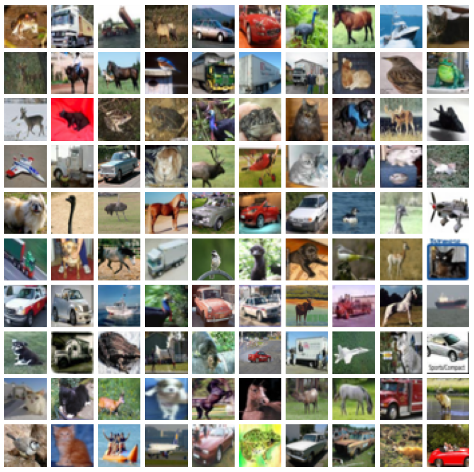
Figure 1. The examples of images from CIFAR-10 dataset [27].
Bdcc 09 00115 g001
Figure 2. MB models with 1 (left) and 3 (right) backbones and the averaging function as a fusion method.
Bdcc 09 00115 g002
Figure 3. MB models with 5 backbones and the averaging function as a fusion method.
Bdcc 09 00115 g003
Figure 4. MB models with 1 (left) or 3 (right) backbones and the dense layer as a fusion method.
Bdcc 09 00115 g004
Figure 5. MB models with 5 backbones and the dense layer as a fusion method.
Bdcc 09 00115 g005
Figure 6. The examples of validation datasets for NN with 3 input channels (ch1–ch3) and backbones: (a) “original”, (b) “simulation” with the same image random orientation across all the channels, (c) “SMA” with the different random image orientations across all the channels, (d) “SMA + simulation” with the same image random orientation and added SMA across all the channels.
Bdcc 09 00115 g006
Figure 7. The examples of validation datasets for NN with 5 input channels (ch1–ch5) and backbones: (a) “original”, (b) “simulation” with the same image random orientation across all the channels, (c) “SMA” with the different random image orientations across all the channels, (d) “SMA + simulation” with the same image random orientation and added SMA across all the channels.
Bdcc 09 00115 g007
Figure 8. The mean (lines) and standard deviation (denoted by background colors and “std” labels in legends) values of validation metrics for the models trained on the original dataset and validated on “SMA” dataset with different number of backbones (N): (a) AUC, (b) accuracy, (c) loss. The legends contain N in the prefix of each label.
Bdcc 09 00115 g008
Figure 9. The mean (lines) and standard deviation (denoted by background colors and “std” labels in legends) values of validation metrics for the models trained on the original dataset and validated on “simulation” and “SMA + simulation” datasets with different number of backbones (N): (a) AUC, (b) accuracy, (c) loss. The legends contain N in the prefix of each label.
Bdcc 09 00115 g009
Figure 10. The best metric values, AUC (a), Accuracy (b), loss (c), for models trained on the original dataset and validated on “SMA” validation dataset and for Averaging (AVG) and Dense (DNN) fusion methods.
Bdcc 09 00115 g010
Figure 11. The best metric values, AUC (a), Accuracy (b), loss (c), for models trained on the original dataset and validated on “simulation” and “simulation + SMA” validation datasets and for Averaging (AVG) and Dense (DNN) fusion methods.
Bdcc 09 00115 g011
Table 1. The best (minimum for Loss, maximum for AUC and Accuracy) metrics values (mean ± standard deviations) for the models trained on the original dataset and validated on “SMA” validation dataset and for various fusion methods (Averaging and Dense).
N_bValidation DatasetFusionAccuracyAUCLoss
1original- 0.615 ± 0.007 0.929 ± 0.002 1.125 ± 0.027
3SMAAveraging 0.415 ± 0.040 0.842 ± 0.010 1.655 ± 0.062
5SMAAveraging 0.436 ± 0.014 0.849 ± 0.004 1.605 ± 0.021
1original- 0 . 621 ± 0.007 0 . 930 ± 0.002 1 . 115 ± 0.020
3SMADense 0.394 ± 0.020 0.819 ± 0.017 1.804 ± 0.117
5SMADense 0.409 ± 0.032 0.838 ± 0.017 1.692 ± 0.075
Table 2. The best (minimum for Loss, maximum for AUC and Accuracy) metrics values (mean ± standard deviations) for models trained on the original dataset and validated on “simulation” and “simulation + SMA” validation datasets and for various fusion methods (Averaging and Dense).
NValidation DatasetFusionAccuracyAUCLoss
1simulation- 0.318 ± 0.008 0.745 ± 0.012 2.218 ± 0.057
3simulation + SMAAveraging 0.347 ± 0.006 0.783 ± 0.005 1.925 ± 0.036
3simulationAveraging 0.323 ± 0.005 0.743 ± 0.007 2.149 ± 0.020
5simulation + SMAAveraging 0 . 350 ± 0.009 0 . 784 ± 0.006 1 . 903 ± 0.034
5simulationAveraging 0.322 ± 0.005 0.740 ± 0.009 2.128 ± 0.033
1simulation- 0.329 ± 0.007 0.750 ± 0.014 2.157 ± 0.080
3simulation + SMADense 0.335 ± 0.008 0.778 ± 0.012 1.931 ± 0.067
3simulationDense 0.325 ± 0.004 0.747 ± 0.007 2.115 ± 0.055
5simulation + SMADense 0.328 ± 0.008 0.768 ± 0.010 1.985 ± 0.035
5simulationDense 0.318 ± 0.005 0.748 ± 0.008 2.153 ± 0.046
Disclaimer/Publisher’s Note: The statements, opinions and data contained in all publications are solely those of the individual author(s) and contributor(s) and not of MDPI and/or the editor(s). MDPI and/or the editor(s) disclaim responsibility for any injury to people or property resulting from any ideas, methods, instructions or products referred to in the content.