Enhancing the FFT-LSTM Time-Series Forecasting Model via a Novel FFT-Based Feature Extraction–Extension Scheme

Abstract

The importance of enhancing the accuracy of time-series forecasting using artificial intelligence tools is increasingly critical in light of the rapid advancements in modern technologies, particularly deep learning and neural networks. These approaches have already shown considerable advantages over traditional methods, especially due to their capacity to efficiently process large datasets and detect complex patterns. A crucial step in the forecasting process is the preprocessing of time-series data, which can greatly improve the training quality of neural networks and the precision of their predictions. This paper introduces a novel preprocessing technique that integrates information from both the time and frequency domains. To achieve this, the authors developed a feature extraction–extension scheme, where the extraction component focuses on obtaining the phase and amplitude of complex numbers through fast Fourier transform (FFT) and the extension component expands the time intervals by enriching them with the corresponding frequency characteristics of each individual time point. Building upon this preprocessing method, the FFT-LSTM forecasting model, which combines the strengths of FFT and Long Short-Term Memory (LSTM) recurrent neural networks, was enhanced. The simulation of the improved FFT-LSTM model was carried out on two time series with distinct characteristics. The results revealed a substantial improvement in forecasting accuracy compared to established methods in this domain, with about a 5% improvement in MAE and RMSE, thereby validating the effectiveness of the proposed approach for forecasting applications across various fields.

1. Introduction

In recent decades, scientific and practical advancements in the field of data analysis and forecasting have made significant progress, largely due to the development of modern technologies, particularly deep learning neural networks. One of the most important tasks in data analysis is time-series forecasting, which involves predicting future values based on historical data [1]. This task is of immense importance across various sectors, including economics, finance, ecology, healthcare, energy, logistics, and many others [2,3,4]. In each of these fields, the accuracy of forecasts directly influences the effectiveness of management decisions, economic indicators, and the responsiveness to changing conditions. Given its significance, time-series forecasting has consistently attracted the attention of researchers and practitioners who aim to enhance forecasting accuracy by employing cutting-edge methods, especially neural network technologies.

Traditional time-series forecasting methods, such as ARIMA (AutoRegressive Integrated Moving Average), exponential smoothing, or regression methods, can be effective under certain conditions [5]. However, they come with a number of limitations, including the need to make assumptions about linearity, stationarity, and other characteristics of the data. In the real world, data can be nonlinear, exhibit complex structures, or feature unpredictable seasonal variations, which makes traditional methods less effective in many cases [6].

Neural networks, especially recurrent neural networks (RNNs) [7] and their variations, such as Long Short-Term Memory (LSTM) and Gated Recurrent Units (GRUs) [8], have significantly improved time-series forecasting results. They are capable of handling large volumes of data, detecting complex dependencies, and accounting for both short-term and long-term relationships. Deep learning models, in particular, can adapt to changes in trends and seasonal fluctuations, making them extremely powerful tools for forecasting [1].

Despite these advancements, improving forecasting accuracy using neural networks still presents certain challenges [9,10]. One of the main challenges is the issue of overfitting, where the model becomes too specialized in learning the training dataset, losing its ability to generalize to new data. Another critical aspect is selecting the appropriate neural network architecture for a specific task. Choosing between simpler and more complex models, as well as tuning parameters such as network depth or the window size for recurrent networks, requires extensive experimentation and time for fine-tuning. Moreover, for these models to work effectively, data preprocessing is a crucial step. High-quality data preparation for neural networks can significantly enhance forecast accuracy, making the consideration of preprocessing methods essential for success in forecasting.

The importance of time-series preprocessing lies in the fact that time-series data often contain various types of noise, missing values, or other anomalies that can negatively affect forecasting performance [11,12]. Despite their power, neural networks are not always capable of efficiently working with unstructured or poorly prepared data [1]. Therefore, preprocessing is critical to achieving high accuracy in forecasting models.

Many time series exhibit seasonal fluctuations—periodic changes that repeat over time [13]. For instance, in economics, seasonal variations can be observed in consumer demand or unemployment rates. Recognizing and adjusting for seasonal components is an essential part of preprocessing. Various methods are used for this, such as decomposing the series into trends, seasonal fluctuations, and residual components, or adjusting or removing seasonal variations to focus on the trend itself. These approaches help make the model more stable and capable of forecasting long-term trends.

Another approach to improving forecasting accuracy, particularly when accounting for seasonality in the data, is the creation of additional features that describe the characteristics of the time series. These features can include changes in values, differences between values over a specific period (e.g., the previous day or month), and lagged variables (values from previous time steps), as well as aggregated characteristics (e.g., average, maximum, or minimum values over a defined period) or frequency characteristics of the signal obtained using various methods [14]. This approach allows neural networks to better understand patterns that may not be immediately obvious when using only the raw data.

A review of the latest scientific works in this field demonstrates the widespread use of LSTM modifications with Fourier transform [15]. A similar approach has been applied to transformer architectures as well [16]. Generalizing these works, the proposed FFT-ANN model suggests replacing each time-series data point with a corresponding frequency characteristic obtained from the Fourier transform, which is then processed by the selected artificial neural network architecture. This approach facilitates the transition from the time domain to the frequency domain for time-series processing, and as shown by the authors [15], it enhances forecast accuracy. However, this approach has several drawbacks, including the following:

• It does not account for the imaginary part of the complex number from Equation (10), i.e., the phase in the polar coordinate system, which also contains important information from the time series and can influence the forecasting accuracy.
• It considers only a single frequency characteristic of the time series, discarding the original time points, which also carry significant information that could improve the forecast accuracy.

Therefore, this paper aims to improve the accuracy of time-series forecasting using neural network methods, particularly through the development of a new feature extraction–extension scheme based on the Fourier transform and its application to enhance the FFT-LSTM time-series forecasting model.

The main scientific contributions of this research can be formulated as follows:

• We developed a new method for preprocessing time-series data, which utilizes information from both the frequency and time domains by employing the feature extraction–extension scheme. In this scheme, the extraction part is responsible for obtaining the phase and amplitude of a complex number via FFT, while the extension part is responsible for expanding the time-series data points with corresponding frequency characteristics for each individual time point of the time series under investigation.
• Based on the developed preprocessing method using the feature extraction–extension scheme, we improved the FFT-LSTM time-series forecasting model, which enhances the accuracy of long-term forecasting tasks.
• We conducted simulations of the enhanced FFT-LSTM time-series forecasting model on two time series with different characteristics and demonstrated improved forecasting accuracy compared to established methods in this class.

The structure of this paper is as follows. Section 2 is dedicated to the review and analysis of existing time-series forecasting methods, with a particular focus on the use of LSTM and its modifications, especially those incorporating time-series preprocessing techniques. Section 3 describes the algorithm of LSTM functionality and its advantages for time-series analysis. The basic mathematical derivations of the Fourier transform, which form the basis of the new time-series preprocessing method with the feature extraction–extension scheme, are provided. The advantages of this approach are substantiated through a mathematical analysis of the algorithm for enhancing the FFT-LSTM time-series forecasting model. Section 4 outlines the datasets used for modeling, justifies the use of various metrics to evaluate the method’s performance, and presents the results on two datasets with different performance indicators. In Section 5, a comparison of the enhanced time-series forecasting model with existing models in this class is conducted. An analysis and discussion of the obtained results are also presented. The summary of the results is provided in Section 6.

2. The State of the Art

Time-series forecasting is not a new problem. There are numerous methods and artificial intelligence tools used to address it. The emergence of deep learning neural networks has given a new impetus to the development of this field. The powerful tools of deep learning provide better forecasting results than many other neural network techniques [17].

A review of the literature reveals that the LSTM architecture and its modifications are widely used for time-series forecasting due to their unique advantages [18,19]. The main feature of LSTM is its ability to retain and transmit information over long periods, thanks to special elements called “memory cells.” This enables LSTM to efficiently process and predict data with long-term dependencies, which is critical for many time-series forecasting tasks, where past values can influence future observations even after a significant period. Additionally, LSTM handles the problem of vanishing and exploding gradients, which often arises in traditional recurrent neural networks (RNNs). Due to its architecture, LSTM can efficiently learn from large datasets, retaining relevant information while discarding irrelevant details. This allows the model to quickly adapt to changes in the data and provide more accurate forecasts. Another important advantage of LSTM is its ability to work with non-stationary data, where statistical properties change over time. This feature is particularly useful for forecasting tasks in financial markets, climate conditions, or energy consumption, where past patterns may change depending on new factors [18,19].

In [20], the authors examined the effectiveness of traditional time-series forecasting techniques, with the ARIMA model showing the highest accuracy. The authors also explored the use of LSTM for solving this task. Experimental modeling demonstrated a significant improvement in forecasting accuracy using the LSTM model compared to all other methods.

In [21], the authors thoroughly analyze the effectiveness of recurrent neural networks (RNNs) and the enhanced Long Short-Term Memory (LSTM) architecture, particularly their ability to model and forecast nonlinear dynamics in time-dependent systems. The review covers existing LSTM cell types and network architectures used for time-series forecasting. The authors propose a classification of LSTM based on optimized cell state representations and models with interacting cell states. According to the study’s findings, “sequence-to-sequence” networks with partial conditional approaches are the most effective, outperforming other models like bidirectional or associative networks in meeting the required performance criteria.

In [22], a modification of LSTM is presented, incorporating a preprocessing method based on the Fourier transform. The authors explored four different combinations of FFT and LSTM results and conducted a series of comparative tests, examining the effectiveness of the procedures when various parameters were altered. The developed approach demonstrated that the combination of FFT-LSTM was more efficient in terms of forecasting horizon and execution time, especially compared to the classical ARIMA model. When compared to similar methods, such as using LSTM alone, the analysis showed that for large datasets and fewer neurons, this approach yielded good results even with a large forecasting horizon. In other words, the combination of the proposed methods not only significantly reduced forecasting errors but also potentially reduced the number of required neurons, speeding up the training process. Furthermore, FFT-LSTM maintained good performance even with long forecasting horizons.

In [23], an improvement to the model from [22] was proposed through optimization of LSTM parameters using the Hyperband model. This approach demonstrated high accuracy in short-term forecasting while solving the applied problem presented by the authors.

Previous studies focused on wavelet transform-based approaches, where wavelet functions were employed to decompose time series into approximation components (low-frequency signals) and detail components (high-frequency signals). Following this decomposition, separate LSTM models were trained on each of these derived signals, and their individual predictions were subsequently combined to produce the final results [24].

Several other works also explore the combined use of FFT and LSTM models for various applications [22,25]. All of them rely on obtaining the most informative frequency characteristics of the signal, which replaces the time series for further analysis. Additionally, the base model in [22] uses only one frequency characteristic of the time series obtained from FFT, which may be insufficient to improve forecasting accuracy for complex time series. Moreover, this model does not utilize information from both the frequency and time domains simultaneously, which could be more informative for artificial neural networks than using only one of them. For these reasons, this work proposes a new feature extraction–extension scheme that addresses the aforementioned limitations of the model from [22] and aims to improve the accuracy of time-series forecasting.

3. Materials and Methods

This section describes the LSTM architecture used for time-series forecasting. The basic principles of Fourier transformation are presented. Based on this, the developed time-series preprocessing method is described, which allows for the incorporation of both frequency- and time-domain characteristics of the series, significantly improving the accuracy of long-term forecasting.

3.1. Long Short-Term Memory Time-Series Forecasting Model

LSTM (Long Short-Term Memory) is a type of recurrent neural network (RNN) specifically designed to overcome the long context size problem that often arises in traditional RNNs when training on long data sequences [20]. Thanks to its unique structure, LSTM is capable of retaining information over extended periods, making it particularly well suited for time-series forecasting tasks. This model is effective at identifying patterns within temporal sequences, allowing it to account for a variety of long-term dependencies in the data.

LSTM consists of several stages, each of which involves three key steps [20]:

• Forget Gate Step—decides which part of the previous state needs to be forgotten. This step is defined by Equation (1):

$$f_t=\sigma (W_f{x}_t+U_f{h}_{t-1}+b_f)$$

(1)

2.

Input Gate Step—determines what new information should be added to the state at the current time step. First, the candidate for the new state is computed using the formula:

$$i_t=\sigma (W_i{x}_t+U_i{h}_{t-1}+b_i),$$

(2)

$${\widehat{c}}_t=tahn(W_c{x}_t+U_c{h}_{t-1}+b_c)$$

(3)

3.

State Update—the state at the current time step is updated considering the information from the forget gate and the input gate:

$$c_t=f_t⨀c_{t-1}+i_t⨀{\widehat{c}}_t$$

(4)

4.

Output Gate Step—determines what information to pass on as output. First, the output gate $\left({\mathrm{o}}_{\mathrm{t}}\right)$ is computed, after which the hidden state $h_t$ is calculated based on the updated state computed in the previous step $c_t$:

$$o_t=\sigma (W_o{x}_t+U_o{h}_{t-1}+b_o),$$

(5)

$$h_t=o_t⨀{tahn(c}_t)$$

(6)

The ability of LSTM to process sequential data and retain long-term dependencies makes it highly effective for time-series forecasting. In time-series data, it is crucial to consider previous observations in order to accurately predict future values. The use of the forget, input, and output gates in the LSTM algorithm allows it to manage information efficiently, either retaining it in the current state or discarding it when it becomes irrelevant. This enables LSTM to avoid the issue of overfitting from long sequences and focus on relevant information, which is particularly important for time series with long-term or seasonal dependencies [20].

3.2. FFT-Based Preprocessing for Time Series

Let us consider a function space, denoted by $\mathrm{X}$, and a transformed function space, denoted by Ψ. Let the function f belong to the space $\mathrm{X}$, i.e., (7):

$$\mathrm{f}\left(\mathrm{t}\right)\in \mathrm{X}$$

(7)

And let the function F belong to the space Ψ, i.e., (8):

$$\mathrm{F}\left(\mathsf{\omega }\right)\in \mathsf{\psi }$$

(8)

The function f is defined as f: R → X, where R is the time space. Therefore, we will assume that the argument of the function f is the time variable t, measured in seconds. The function F is defined as F: Z → ψ, where Z is the complex space. Thus, we consider the argument of the function F to be the frequency variable ω, measured in radians per second. We define a functional transformation φ from the space X to the space ψ as follows (9):

$$\mathrm{f}:\mathbb{R}\to \mathrm{X}$$

(9)

Let us examine types of transformations of the form (9):

• A special case of the general transformation of the form (9) is the continuous one-dimensional Fourier transform, given by the following formula:

$$\mathrm{F}(\mathsf{\omega })={\int }_{-\mathrm{\infty }}^{\mathrm{\infty }}\mathrm{f}(\mathrm{t}){\mathrm{e}}^{-\mathrm{i}\mathsf{\omega }\mathrm{t}} \mathrm{d}\mathrm{t}$$

(10)

2.

Another special case of the transformation of the form (9) is the discrete one-dimensional Fourier transform, which is applied for processing discrete output signals in the time space Χ. The discrete Fourier transform, similar to its continuous counterpart, transforms the time space Χ into the frequency space Z.

A feature of applying the discrete Fourier transform is the use of discrete sequences of output data, particularly time series that can be either finite or infinite. The discrete Fourier transform for a finite numerical series with N samples is defined as follows:

$$X_k={\sum }_{n=0}^{N-1}{x}_n{e}^{-ikn{\displaystyle \frac{2\pi }{N}}}, k=0, 1, 2,\dots , N-1,$$

(11)

x—input sequence (discrete signal).

$X_k$—spectral parameters resulting from the discrete Fourier transform.

N—number of samples (length of the discrete sequence).

Let us consider the set of spectral parameters {$X_k$, k = 0, 1, 2,…, N − 1}, which contain information about the signal’s frequency components. Since the set of spectral parameters is a subset of the complex number space Z, which is the Cartesian product of the real and imaginary axes, for each spectral parameter $X_k$, the following formula holds:

$$X_k=Re\left(X_k\right)\pm iIm\left(X_k\right), k=\mathrm{0,1},2,\dots ,N-1$$

(12)

To transmit and process spectral parameters in a neural network-based model, we represent them using the polar form of a complex number:

$$X_k=\left|X_k\right|\left(cos\right(arg\left(X_k\right))+isin(arg\left(X_k\right)\left)\right),$$

(13)

where

$$\left|X_k\right|=\sqrt{Re{\left(X_k\right)}^2+Im{\left(X_k\right)}^2},$$

(14)

$$\mathrm{a}\mathrm{r}\mathrm{g}\left(X_k\right)=\mathrm{a}\mathrm{r}\mathrm{c}\mathrm{t}\mathrm{a}\mathrm{n}\left({\displaystyle \frac{\mathrm{I}\mathrm{m}\left(X_k\right)}{\mathrm{R}\mathrm{e}\left(X_k\right)}}\right)$$

(15)

This means that instead of using Formula (12), we use Formulas (13)–(15), where each spectral parameter is described by two quantities uniquely calculated based on the polar form of a complex number.

Formula (14) defines the modulus (magnitude of the complex number), which characterizes the amplitude of the spectral parameter. Formula (15) calculates the argument (angle of the complex number), which specifies the phase of the spectral parameter. The values of the modulus and argument more clearly represent the signal’s frequency characteristics because they directly determine its amplitude and phase.

The values of the modulus and argument of the spectral parameters are used as input data for further time-series analysis based on machine learning methods.

3.3. Improvement of the FFT-LSTM Model Through the FFT-Based Feature Extraction–Extension Scheme

After transforming time-series data using the discrete Fourier transform (DFT), there are various approaches to representing the obtained data in a machine learning model. Specifically, in [22], an approach is described that involves using only the real part of the Fourier transform (as in Equation (14)) to replace the time-series values. This approach allows for a transition from the time domain to the frequency domain for time series processing and as shown by the authors, improves forecasting accuracy. However, this approach has several drawbacks, which were discussed in Section 1. To address these limitations, this section proposes an enhancement to the time-series preprocessing method using Fourier transform, which improves the accuracy of long-term forecasts. The whole scheme of the proposed model is shown in Figure 1.

According to the proposed method, both the time-series values and frequency characteristics obtained through the Fourier transform, specifically the phase and amplitude, are fed into the model. This allows the model to simultaneously work with information from both the time domain and the frequency domain. As a result, the model receives a more complete representation of the signal, as it has access to both its original values and their frequency properties.

The phase encodes the temporal alignment of frequency components. Ignoring the phase results in critical information about when specific frequency patterns occur in the time series to be discarded. For example, two signals with identical amplitude spectra but different phases will behave entirely differently in the time domain. Without the phase, the model cannot distinguish between such cases, leading to suboptimal predictions.

Let us present the mathematical description of the data representation in the model according to the FFT-based feature extraction–extension scheme as follows:

$$t_1,{ t}_2,\dots , t_n\to t_1, A_1,{ \phi }_1, t_2,{ A}_2,{ \phi }_2,\dots ,t_n,{ A}_n,{ \phi }_n,$$

(16)

where

$t_1,{ t}_2,{\dots ,t}_n$ are points in the time domain;

${\mathrm{A}}_1,{\mathrm{A}}_2,{\dots , A}_n$ are amplitudes obtained after the discrete Fourier transform;

${\mathsf{\phi }}_1,{\mathsf{\phi }}_2,{\dots ,\phi }_n$ are phases obtained after the discrete Fourier transform.

The proposed approach is based on the modification of the FFT-LSTM method, which was introduced in [22]. To demonstrate how this approach can be beneficial for LSTM, it is important to consider a model that utilizes both time and frequency characteristics to enhance its performance.

We will describe step by step the data processing based on the enhanced FFT-LSTM time-series forecasting model. The first hidden state is defined as follows:

$$h_t=\left[x\left(t\right),A_t,{\phi }_t\right]$$

(17)

Thus, the forget gate step from Formula (6) will include the amplitude and phase from the previous step:

$$f_t=\sigma (W_f·\left[x_t,A_t,{\phi }_t\right]+U_f·\left[x_{t-1},A_{t-1},{\phi }_{t-1}\right]+b_f)$$

(18)

The updated cell state from Formula (9) will look like this:

$${\widehat{c}}_t=tahn(W_c·\left[x_t,A_t,{\phi }_t\right]+U_c·\left[x_{t-1},A_{t-1},{\phi }_{t-1}\right]+b_c)$$

(19)

And the amplitudes and phases from the time series will proceed to the last step in the network according to (10):

$$o_t=\sigma (W_o·\left[x_t,A_t,{\phi }_t\right]+U_o·h_{t-1}+b_o)$$

(20)

Thus, we can see that at each step, the LSTM will compare data from previous steps not only based on the time-series values but also using its two frequency characteristics (amplitude and phase), defined through discrete FFT. This approach will provide additional information to the neural network through the frequency characteristics, while also allowing the inclusion of the original time series in the time domain. Collectively, this method will enhance forecasting accuracy in the long-term period for time series across various application domains.

4. Modeling and Results

This section is dedicated to describing the datasets used for modeling the performance of the proposed method, outlining the metrics for evaluating the model’s effectiveness, and presenting the results of the developed approach.

4.1. Datasets

The modeling was conducted on two datasets that covered various time series with different measurement frequencies and specific characteristics.

The first dataset contains information on wind energy production in MW, recorded every 4 s, starting from 8 January 2019. The total length of this time series is 7,397,147 data points. The context size for this dataset is 60 time points, corresponding to 4 min of data. Although the data have a high-frequency nature, our goal is to use them for long-term forecasting of wind energy production. This is crucial for energy planning and ensuring the stability of the power grid over longer time intervals. This dataset is available in a public repository and can be downloaded here [26].

The second dataset contains daily total sunspot numbers, spanning from 1818 to the present day. This dataset represents a long-term time series that allows for the analysis of long-term trends in solar activity. The context size for this dataset is 30 time points (days), meaning that when making predictions, we consider data from the previous 30 days. This enables the model to capture monthly cycles and seasonal fluctuations, which is essential for accurate long-term forecasting of sunspot activity. This dataset is available in a public repository and can be downloaded here [27].

4.2. Performance Indicators

The modeling of the proposed approach was carried out using a number of important metrics to provide a comprehensive evaluation of its effectiveness. Among them, the following should be highlighted:

• Mean Absolute Scaled Error (MASE)

$$\mathrm{M}\mathrm{A}\mathrm{S}\mathrm{E}={\displaystyle \frac{\frac{1}{\mathrm{n}}{\sum }_{\mathrm{t}=1}^{\mathrm{n}}\left|{\mathrm{a}}_{\mathrm{t}}-{\widehat{\mathrm{a}}}_{\mathrm{t}}\right|}{\frac{1}{\mathrm{n}-\mathrm{m}+1}{\sum }_{\mathrm{t}=\mathrm{m}+1}^{\mathrm{n}}\left|{\mathrm{a}}_{\mathrm{t}}-{\widehat{\mathrm{a}}}_{\mathrm{t}-\mathrm{m}}\right|}}$$

(21)

• Symmetric Mean Absolute Percentage Error (SMAPE)

$$\mathrm{S}\mathrm{M}\mathrm{A}\mathrm{P}\mathrm{E}={\displaystyle \frac{100\%}{\mathrm{n}}}{\sum }_{\mathrm{t}=1}^{\mathrm{n}}{\displaystyle \frac{\left|{\mathrm{a}}_{\mathrm{t}}-{\widehat{\mathrm{a}}}_{\mathrm{t}}\right|}{\frac{\left|{\mathrm{a}}_{\mathrm{t}}\right|+\left|{\widehat{\mathrm{a}}}_{\mathrm{t}}\right|}{2}}}$$

(22)

• Mean Absolute Error (MAE)

$$\mathrm{M}\mathrm{A}\mathrm{E}={\displaystyle \frac{1}{\mathrm{n}}}{\sum }_{\mathrm{t}=1}^{\mathrm{n}}\left|{\mathrm{a}}_{\mathrm{t}}-{\widehat{\mathrm{a}}}_{\mathrm{t}}\right|$$

(23)

• Mean Squared Error (MSE)

$$\mathrm{M}\mathrm{S}\mathrm{E}={\displaystyle \frac{1}{\mathrm{n}}}{\sum }_{\mathrm{t}=1}^{\mathrm{n}}{({\mathrm{a}}_{\mathrm{t}}-{\widehat{\mathrm{a}}}_{\mathrm{t}})}^2$$

(24)

• Root Mean Squared Error (RMSE)

$$\mathrm{R}\mathrm{M}\mathrm{S}\mathrm{E}=\sqrt{{\displaystyle \frac{1}{\mathrm{n}}}{\sum }_{\mathrm{t}=1}^{\mathrm{n}}{({\mathrm{a}}_{\mathrm{t}}-{\widehat{\mathrm{a}}}_{\mathrm{t}})}^2}$$

(25)

where ${\mathrm{a}}_{\mathrm{t}}$ is the real value, ${\widehat{\mathrm{a}}}_{\mathrm{t}}$ is the predicted value, $\mathrm{m}$ is the context size of the predicted values, and $\mathrm{n}$ is the size of the test dataset.

The use of MASE allows for comparison of models across different datasets, as it is scale-independent. SMAPE, on the other hand, takes into account the absolute deviations between the forecast and actual values, normalizing them by the sum of their absolute values, which provides a symmetric evaluation of relative errors. The application of MAE enables the assessment of the average deviation of the forecast from the actual values, with the result being interpreted in the same scale as the original data. MSE provides an evaluation of larger deviations in forecasts, as it considers the mean squared error. RMSE offers a clear understanding of the average magnitude of errors, placing more emphasis on larger errors, making it useful not only for assessing accuracy but also for detecting the stability of the model.

4.3. Results

The modeling was carried out using two datasets. The results obtained based on the use of Equations (21)–(25) are presented in

Table 1. The results of the enhanced FFT-LSTM time-series forecasting model on two time series with different characteristics are presented in Table 1.

Errors/Dataset	Dataset 1	Dataset 2
MASE	0.97	0.95
SMAPE	0.76	0.72
MAE	3.24	2.21
MSE	14.04	7.95
RMSE	3.7	2.82

.

As seen from the results in Table 1, the enhanced FFT-LSTM time-series forecasting model demonstrated high accuracy in short-term forecasting, based on the analysis of all performance metrics (21)–(25). However, to assess its effectiveness, a comparison of its accuracy with that of well-known methods in this class was performed.

5. Comparison and Discussion

To evaluate the effectiveness of the enhanced FFT-LSTM time-series forecasting model using the FFT-based feature extraction–extension scheme, the prediction errors of this method were compared with the errors of existing methods. Among the existing methods, two were selected from the same class. The first is the classical LSTM model [18], which is widely used for long-term time-series forecasting tasks. It operates in the time domain, allowing the model to account for temporal changes and potentially important trends or patterns in the time series. The second method is based on the FFT-LSTM time-series forecasting model [22], which involves transforming the time-series data into the frequency domain by replacing time-sequence values with a single frequency characteristic derived from the real part of a complex number (14). This method works in the frequency domain, making it capable of detecting periodic components that might be crucial for forecasting.

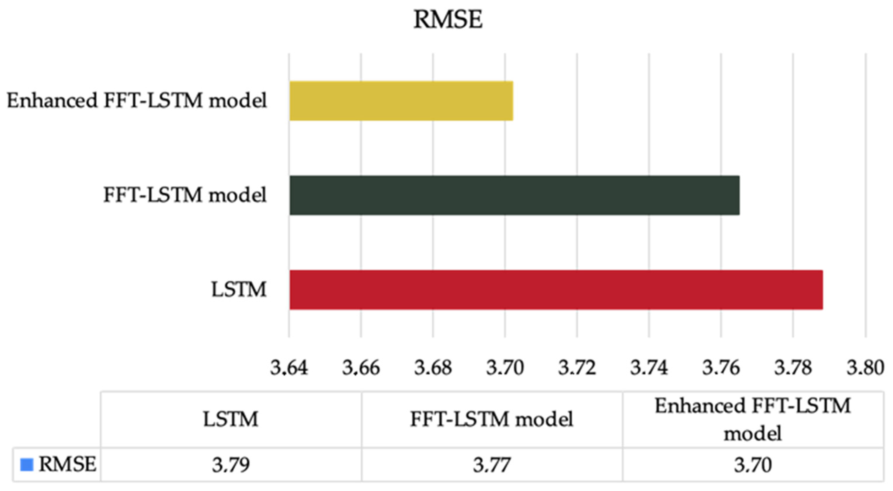
Figure 2 shows the RMSE values when applying the two existing methods (LSTM and FFT-LSTM) and the enhanced method on the first dataset.

As seen from the results in Figure 2, the lowest accuracy is demonstrated by the time-series forecasting model based on LSTM. A slightly higher accuracy is achieved by transitioning from the time domain to the frequency domain using the FFT-LSTM model. However, the difference is not very large.

A significantly lower RMSE value is obtained when using the enhanced FFT-LSTM time-series forecasting model with the FFT-based feature extraction–extension scheme developed in this study. Specifically, this model shows a 2.2% higher accuracy compared to the LSTM model and a reduction of over 1.5% in RMSE compared to the FFT-LSTM model. All other error metrics also demonstrate similar results, confirming the effectiveness of the enhanced approach.

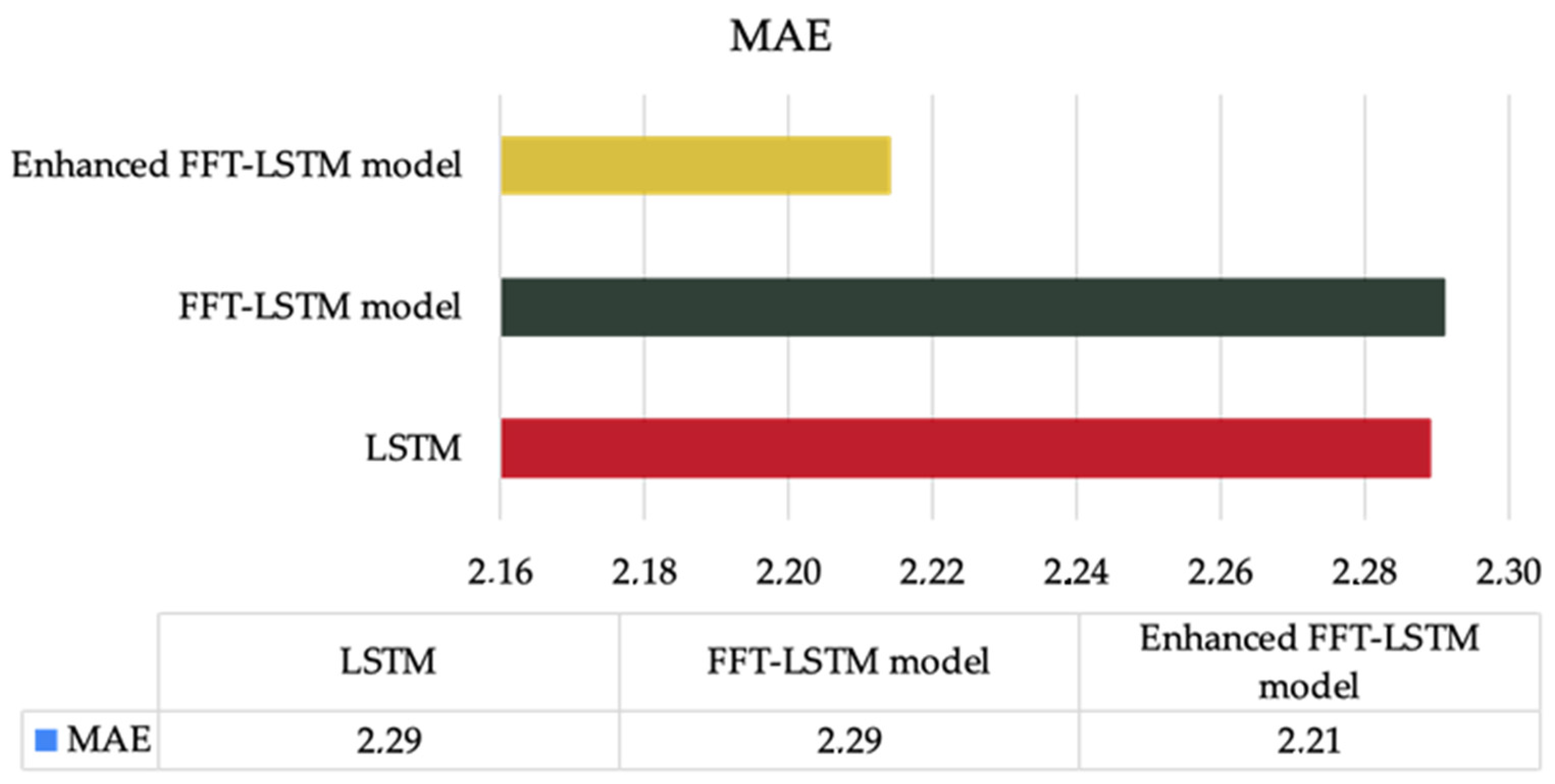
Figure 3 shows the results (based on MAE) for the use of all three investigated methods with the second dataset.

As seen from the results presented in Figure 3, as in the previous case, the lowest short-term forecasting accuracy was achieved using the classical LSTM model. However, when analyzing this dataset, it is evident that the application of FFT-LSTM slightly worsened the forecasting accuracy, especially when compared to the LSTM model. This suggests that using only one frequency characteristic of the time series, and replacing the original data with it, does not always provide sufficient information for the artificial neural network.

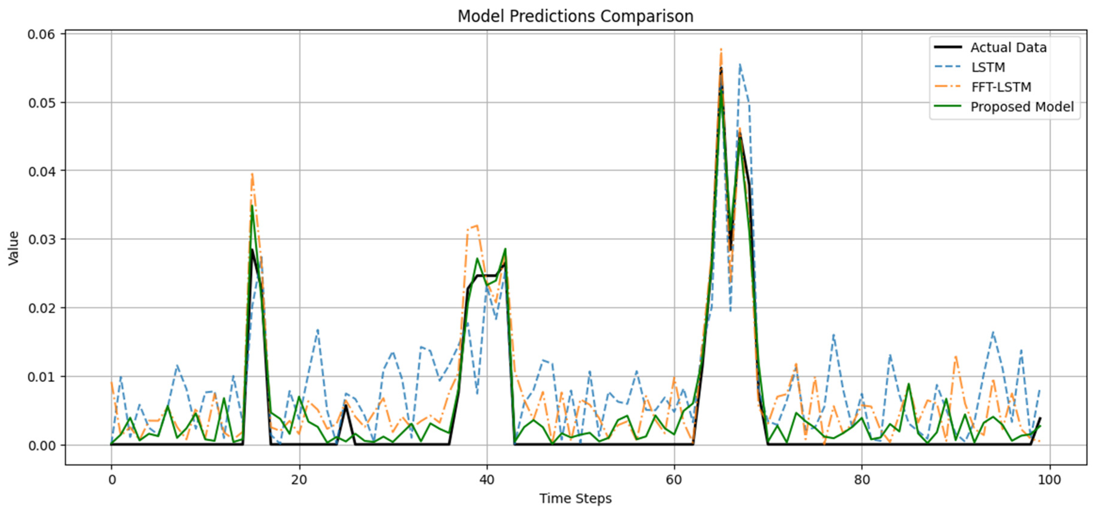
Significantly lower errors in solving this task were obtained by using the enhanced FFT-LSTM time-series forecasting model with the FFT-based feature extraction–extension scheme proposed in this work. Specifically, it demonstrates more than a 3% reduction in MAE compared to the existing methods. Also, for demonstration of the forecasts generated by the proposed model in comparison with LSTM and FFT-LSTM, Figure 4 provides a comparison of the first dataset and Figure 5 provides a comparison of the second dataset. Also, to understand the time complexity of the models, we created

Table 2. Time complexity of compared models.

Metrics/Models	Proposed Model	FFT-LSTM	LSTM
Training time	185 min	185 min	190 min
Inference time	0.5 s	0.5 s	0.5 s

.

Summarizing the obtained results, the following conclusions can be made:

• The enhanced FFT-LSTM time-series forecasting model using the FFT-based feature extraction–extension scheme proposed in this work combines the advantages of both approaches mentioned above, as it allows for analyzing the time series from both the time and frequency domains simultaneously.
• By using the preprocessing method developed in this work, the enhanced FFT-LSTM time-series forecasting model can now account for both temporal changes and cyclic patterns. This enables it to better understand complex dependencies in the data, which in turn allows for more accurate predictions of future values for complex time series.
• The existing FFT-LSTM time-series forecasting model does not always guarantee improved forecasting accuracy, especially in the case of Dataset 2. This is due to the complexity of this time series and the use of a limited number of frequency characteristics (only 1), which suppresses important information from the frequency domain of the time series.
• The results of practical experiments on both datasets, using various performance metrics, confirm the improvement in forecasting accuracy based on the enhanced model presented in this work, compared to models that only operate in either the time or frequency domain.
• In theory, the preprocessing method based on the feature extraction–extension scheme developed in this work can be used to improve forecasting accuracy in other neural network architectures as well. However, this requires further investigation.

Among the drawbacks of the enhanced model, a significant one is the increased size of the time window used for modeling, due to the need to account not only for each individual time step but also for its frequency characteristics—phase and amplitude—obtained using Fourier transform. To mitigate this limitation, various techniques for optimizing processing time and reducing model complexity can be applied, including adaptive windows, input size reduction, the use of faster algorithms, or parallel computing. Additionally, the ongoing advancement of computational power somewhat alleviates this issue, and the need for highly accurate forecasts in critical tasks may prioritize the goal of achieving high precision over minimizing computational costs. This would allow the use of the enhanced model proposed in this work in practical applications.

Future research will focus on two main directions:

• Research on the effectiveness of using the developed time-series preprocessing method with the feature extraction–extension scheme in other artificial neural network architectures.
• Development of methods for extracting frequency characteristics of time series based on wavelet transforms, and their use for improving the accuracy of both short-term and long-term time-series forecasting.

6. Conclusions

Modern artificial intelligence methods, particularly deep neural networks, have gained significant popularity for solving time-series forecasting problems due to their ability to efficiently process large volumes of data and uncover complex patterns that may remain unnoticed by traditional approaches. One of the critical stages in the forecasting process is data preprocessing, which plays a decisive role in improving the quality of neural network training and ensuring more accurate predictions.

This article proposes a novel time-series preprocessing method that combines information from both the time and frequency domains. This approach significantly enhances the FFT-LSTM forecasting model, which combines the advantages of the fast Fourier transform and recurrent neural networks (LSTM). The modeling of the improved model was conducted on two different time-series datasets, and the experimental results confirmed a significant increase in forecasting accuracy compared to other known methods, demonstrating the high effectiveness of the proposed approach for forecasting tasks.

The results of the study allow for several key conclusions. First, combining data processing in both time and frequency domains in the FFT-LSTM model leads to a substantial improvement in forecasting accuracy. Second, the use of the time-series preprocessing method enables the model to account for both temporal changes and cyclical patterns in the data, thereby improving forecasting accuracy for complex time series.

Experimental results demonstrate that the enhanced model provides higher accuracy (by 2–3%) compared to other approaches that operate in just one domain—either time or frequency. However, there is a certain drawback in the form of an increased size of the time windows required to account for frequency characteristics. Due to the development of computational power, this limitation is becoming less of a concern, as modern technologies allow for the application of complex models without significant processing time losses.

Further research should focus on two main directions: improving the time-series preprocessing method for use in other artificial neural network architectures and developing new methods for extracting the frequency characteristics of time series, particularly based on wavelet transforms, to improve forecasting accuracy for long-term periods.