Abstract
Integrating deep learning into microbiological and cell analysis from microscopic image samples has gained significant attention in recent years, driven by the rise of novel medical technologies and pressing global health challenges. Numerous methods for segmentation and classification in microscopic images have emerged in the literature. However, key challenges persist due to the limited development of specialized deep learning models to accurately detect and quantify microorganisms and cells from microscopic samples. In response to this gap, this paper introduces MBnet, an Extreme-Lightweight Neural Network for Microbiological and Cell Analysis. MBnet is a binary segmentation method based on a Fully Convolutional Network designed to detect and quantify microorganisms and cells, featuring a low computational cost architecture with only 575 parameters. Its innovative design includes a foreground module and an encoder–decoder structure composed of traditional, depthwise, and separable convolution layers. These layers integrate color, orientation, and morphological features to generate an understanding of different contexts in microscopic sample images for binary segmentation. Experiments were conducted using datasets containing bacteria, yeast, and blood cells. The results suggest that MBnet outperforms other popular networks in the literature in counting, detecting, and segmenting cells and unicellular microorganisms. These findings underscore the potential of MBnet as a highly efficient solution for real-world applications in health monitoring and bioinformatics.
1. Introduction
Microscopic sample analysis involves various methods used to detect, identify, and quantify microscopic biological entities such as bacteria, viruses, yeast, blood cells, and malignant cells. In recent years, interest in these fields has grown due to their pivotal role in the Medical Internet of Things (IoMT), telemedicine, clinical laboratory research, and responses to global health challenges such as the COVID-19 pandemic and antibiotic resistance. Traditionally, these analyses have relied heavily on human inspection, image processing, or semi-automated procedures that require costly technologies. However, these methods remain highly susceptible to human error, potentially leading to misdiagnosis and data mishandling. To address these challenges, since the early 2010s more researchers have been turning their attention to deep learning (DL) models in order to analyze cells from microscopic sample images [1]. These DL approaches offer superior accuracy and processing speed compared to traditional methods. Consequently, DL has led the way for new microbiological, hematological, and histological research applications, providing fresh perspectives and driving discoveries in the field [2].
Today, many researchers utilize artificial intelligence (AI) to enhance the analysis of microscopic biological entities in microbiology, hematology, and histology. These disciplines focus on studying different types of microorganisms and cells in order to generate clinical reports that assess an individual’s health status. AI has significantly improved and accelerated clinical analysis in laboratories and hospitals, primarily through the use of DL for interpreting images of microscopic samples. In microbiology, researchers study microorganisms, and DL has been applied to analyze microscopic culture plates containing bacteria, fungi, algae, parasites, protozoa, and viruses [1,3,4,5,6]. Hematology examines blood cells and their components such as hemoglobin, while histology delves into the microscopic structure of cells, tissues, and organs, providing information on their organization and function. DL has also been implemented to analyze hematologic and histologic samples, including blood cells and malignant cells, which helps to diagnose a variety of pathologies [7,8].
Microbiological, hematological, and histological analyses are increasingly utilizing DL methods for improved accuracy and efficiency. These methods play a crucial role in counting, segmenting, and classifying microorganisms and cells. In terms of counting, the process involves quantifying microscopic entities such as bacteria, viruses, yeast, and blood cells. This quantification provides essential data for a variety of applications. Effective counting methods range from classical techniques to advanced algorithms such as Support Vector Machine (SVM), Multi-Layer Perceptron (MLP), and Convolutional Neural Network (CNN) [3]. Segmentation techniques accurately detect cells and outline their morphology, which is vital for identifying microorganisms and malignant cells. Leading methods in this area include UNet, UNet++, and DeepLab [5]. For classification, the goal is to identify and categorize microorganisms and cells such as bacteria, fungi, malignant cells, and blood cells. This process is essential for both research and clinical diagnostics. Techniques such as K-Nearest Neighbor (KNN), Random Forest (RF), and CNN are used for classification [1,6]. Integrating DL into these analyses can streamline processes and improve accuracy, contributing to microbiological and clinical research advancements.
According to a review and analysis of the literature, DL models are currently able to effectively detect, quantify, and classify microbiological and cellular entities from microscopic sample images. However, these models come with high computational costs, require large datasets for training, and are often designed to address specific tasks in histological, microbiological, or hematological studies. Another challenge is that most studies focus on classifying microorganisms or cells from manually cropped images obtained from raw microscope images. Therefore, it is crucial to develop low-cost DL models capable of learning multiple tasks and being trained on a limited number of raw image samples. To address these challenges, this paper proposes a novel model called Extreme-Lightweight Neural Network for Microbiological and Cell Analysis (MBnet) an FCN with significantly lower computational cost designed for binary semantic segmentation of any microorganism or cell from raw images obtained in microbiological, hematological, or histological studies. The segmentation process is applied to detection and quantification tasks in which the foreground consists of microscopic biological entities such as microorganisms, cells, and other microbiological entities to be segmented, while the rest of the raw image is considered background.
MBnet consists of traditional, depth-wise, and separable convolution layers organized into a foreground module analysis and an encoder–decoder architecture, all while utilizing only 575 parameters. This architecture significantly reduces hardware resource consumption compared to the traditional DL models commonly employed in microbiological, hematological, and histological analyses. Additionally, MBnet requires fewer training samples than typical DL models. Experiments with MBnet were conducted using three datasets that included microscopic samples of bacteria, yeast, and blood cells. The layers of MBnet integrate color, morphological, and orientation patterns in order to understand the context of the microscopic image and separate the background and the cells or microorganisms to be segmented. The primary application of this network is the detection and quantification of microscopic biological entities, which often pose challenges in analyses within clinical laboratories, telemedicine, bioinformatics applications, IoMT, and medical diagnostics.
The rest of this paper is organized as follows: Section 2 reviews the current state of the art related to this work; Section 3 describes the architecture of MBnet and its feature maps; Section 4 outlines the dataset used for the experiments; Section 5 presents the results and discussion; finally, Section 6 concludes the paper.
2. Related Work
The state of the art presented in this work compiles recent research on microorganisms and cell analysis using DL. In summary, the reviewed studies propose using networks such as UNet, Recurrent CNN (R-CNN), or CNN to analyze microscopic images of bacteria, yeast, parasitic diseases, and cell morphology. A brief description of these investigations is provided below.
Regarding bacterial analysis, Park et al. developed a method for segmenting bacteria using hyperspectral images and UNet-based models in [9]. The Attention-Gated Recurrent Residual UNet (AGR2U-Net) demonstrated the best processing time compared to other UNet models, achieving an IoU of 94.1%. Ferrari et al. proposed a CNN in [10] for counting and classifying bacterial colonies in Petri dishes, with results showing precise colony counts and a classification accuracy of 97% that outperformed traditional manual methods. In [11], Sun et al. introduced a hybrid UNet-based model combined with DropBlock for bacterial segmentation from simulated Raman scattering microscopy images. Their method offers improved segmentation and enables single-cell metabolic inactivation concentration calculations in under one minute, whereas other methods require up to 40 min. In [12], Zou et al. reported a Mask-RCNN for analyzing bacterial communities in soil samples via microfluidic chips collected from Greenland, Sweden, and Kenya. This Mask-RCNN segments and classifies individual bacteria, dividing bacteria, and bacterial clusters, achieving accuracy results of 90% to 91% and recovery rates of 94% to 96%. Their data revealed significant bacterial density and morphology differences across the three regions. In [13], Kanchanapiboon et al. presented a Faster R-CNN for evaluating the severity of Orientia tsutsugamushi bacterial infectivity using instance segmentation. Experiments conducted on fluorescent scrub typhus images from molecular screening highlighted the potential of this integrated approach to enhance accuracy and efficiency in bacterial infectivity evaluations within molecular research.
In yeast analysis, Prangemeier et al. introduced a modified UNet and Mask R-CNN for segmenting yeast cells and microstructures [14]. These models achieved impressive accuracy, with a Dice coefficient of 0.96 and an IoU score of 0.89, outperforming existing state-of-the-art methods. Similarly, Ghafari et al. [15] conducted a comparison between a CNN, a Capsule Neural Network (CapsNet), and a hybrid CNN–CapsNet architecture for classifying yeast in microfluidic images at various stages of the replicative aging process. While the CNN surpassed CapsNet in terms of overall accuracy, CapsNet demonstrated greater robustness in detecting specific categories. The hybrid CNN–CapsNet model achieved the highest overall accuracy at 98.5%.
In analyzing parasitic diseases, Hung et al. developed a Python library using Keras R-CNN for detecting and classifying cells in biological images [16]. This approach achieved an average accuracy of 82% in nuclei detection and 78% in classifying the stages of malaria caused by Plasmodium vivax. In [17], Preißinger et al. introduced CNN-based software for detecting and classifying malaria stages in red blood cells, reaching an accuracy of 96%. Their method significantly improved the speed and accuracy of malaria stage detection and classification in microscopy images. In [18], Maity et al. developed a segmentation method based on CapsNet for identifying malaria from parasite-infected red blood cell images, achieving an accuracy of 98.7% for detecting infections caused by Plasmodium vivax and Plasmodium falciparum. Additionally, Libouga et al. [19] proposed a UNet model for segmenting and classifying four types of human intestinal parasites (Ascaris lumbricoides, Schistosoma mansoni, Trichuris trichiura, and Oxyuris). Their model demonstrated a detection accuracy of 99.8% on a dataset comprising 320 color microscope images.
In cell morphology analysis, Halima et al. introduced a novel method for cell deformability segmentation and detection in microscopic images using UNet [20]. Their method achieved an accuracy of 81%, improving cellular deformability detection without the need for expensive materials or expert intervention. In [21], Cicatka et al. proposed two new annotated datasets and a novel UNet-based methodology for generating synthetic agar plates. The datasets consisted of 854 images of cultivated agar plates and 1588 images of empty agar plates featuring different microorganisms. Their model achieved a Dice coefficient of 0.729 with this dataset. In [22], Karabağ Cefa et al. evaluated the impact of training data volume and shape variability on HeLa cell segmentation using UNet. Electron microscopy images and label pairs were generated to train different UNet architectures, with the results indicating that increased training data and cellular diversity improved both the accuracy and IoU score. Their study concluded that combining different data sources enhances segmentation results. Lastly, Mohammed et al. [23] assessed the performance of several models (UNet, UNet++, Tiramisu, and DeepLabv3+) for microscopic image segmentation. They also proposed a new model called PPU-Net, which achieved comparable performance to the others but with 20 times fewer parameters.
3. MBnet
The most commonly used DL models for detecting and quantifying biological entities include traditional CNN architectures such as MobileNet, ResNet, YOLO, and VGG. The most frequently employed models for segmentation tasks are UNet, FCN, and Mask R-CNN. However, standard CNN architectures tend to be very deep, and are primarily designed for classification, which means that they extract numerous abstract features.
FCN and Mask R-CNN are specialized in segmentation but have high computational costs due to their relationship with deep CNN architectures. These models often incorporate transposed convolutional layers or attention mechanisms, increasing their complexity. In particular, Mask R-CNN is designed for instance segmentation, enabling the identification of internal structures within microorganisms and cells. On the other hand, UNet-based models are popular for segmentation tasks but struggle with class imbalance and exhibit high computational complexity.
Based on this analysis, we conclude that CNNs and FCNs have high computational costs due to their dependence on traditional deep CNN architectures. UNet faces challenges related to computational complexity, while Mask R-CNN is tailored specifically for instance segmentation. This conclusion leads to the hypothesis that it should be possible to design a deep neural network for cell detection and quantification that significantly reduces computational costs. This can be achieved by creating an FCN with a novel convolution configuration capable of extracting suitable features for binary segmentation. MBnet was developed based on this hypothesis, which is described in detail below.
Figure 1 illustrates the architecture of MBnet, which is divided into four main components: the input, foreground module, FCN, and output. The input consists of a microscopic sample image, while the foreground block enhances the features of biological entities. The FCN is further divided into three parts, the encoder, bottleneck, and decoder, which work together to suppress the background of the image. The output produces the segmentation of microscopic biological entities for detection and quantification. The following subsections provide details on the training process, convolution layers, and architecture of MBnet. This supervised learning process allows MBnet to understand the context of microscopic sample images.
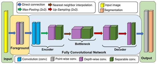
Figure 1.
MBnet architecture.
3.1. Training
The foreground block and FCN layers consist of convolutional neurons trained using mini-batch gradient descent with a batch size of 10, a binary focal cross-entropy (BFCE) loss function, and a learning rate of 0.01. Mini-batch gradient descent and the selected batch size were chosen in order to provide effective generalization with small sample sizes [24]. BFCE was selected because it is explicitly designed for datasets with imbalanced binary classes. This is advantageous for MBnet because microorganisms, cells, and tissues often occupy a significantly smaller area than the background, resulting in class imbalance [25].
3.2. Convolution Layers
The layers of MBnet are composed of traditional convolution, depthwise, and pointwise convolution layers. The traditional convolution layers are defined as follows:
where is the layer index, is the depth of the layer , is the bias, is the output of the last layer, and is the output.
The pointwise convolution is a convolution defined by Equation (1), where the size of is , the bias is zero, and the activation function is provided by . Therefore, the pointwise convolution can be represented as
The weights in Equation (2) adjust the contribution of the channels from the previous layer and are trained using the method detailed in Section 3.1. The depthwise convolution layer applies a separate convolution filter to each channel of the last layer. This convolution is defined as
The separable convolution reduces the number of training parameters by two steps: a depthwise convolution defined in Equation (3), followed by a pointwise convolution described in Equation (2). The depthwise separable convolution is then defined as follows:
where is the kernel that defines the operation of Equation (2).
Traditional convolution layers are used in the first encoder layers due to their ability to effectively capture low-level features. On the other hand, depthwise and separable convolutions are optimized implementations of the convolution operation used in the remaining FCN layers. These approaches generate different features while significantly reducing the number of parameters [26,27].
The activation function in Equations (1) and (3) is a leakyReLU function, defined in [28]. leakyRELU was selected because of its better ability to detects he morphological features of microorganisms and cells compared other activation functions. In addition, it manages the gradient vanishing problem more suitably due to the reduced number of layers.
3.3. Architecture
This section describes the architecture of MBnet and the activation maps of its layers, using an image of a microscopic sample of blood cells as input. This description is supported by the visualization of false color activation maps obtained during the propagation of an image (named 0010.png in this article).
3.3.1. Input and Foreground Module
The input is a color image with a size of , where represents the spatial resolution. This resolution was selected because according to our experiments it is sufficient to represent the morphology of biological entities in histological, blood smear, and microbiological culture samples. Figure 2 shows an example of a microscopic sample image containing blood cells, where is the red channel, is the green channel, and is the blue channel.
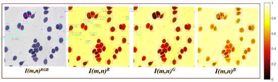
Figure 2.
An input example with blood cells (erythrocytes and leukocytes); is presented in real color, while the color channels are represented in false color.
The foreground module stimulates the cells or microorganisms to be detected, and compresses into a single component channel. The first layer applies a depthwise convolution as described by Equation (3), where the input is . This depthwise convolution is followed by a pointwise convolution, as defined in Equation (2), where . The output is a new component with and a size of .
Layer learns to separate the background and foreground in different channels. The module can achieve this separation because the learned weights of Equation (3) increase the variance between background and foreground features. For example, Figure 3 shows that the feature map inhibits the foreground and inhibits the background. Additionally, captures the maximum values of the RGB channels in each pixel. Layer adds the three channels of using Equation (2), compressing into a single channel that preserves the variance between foreground and background features. This feature compression in is achieved because of the pointwise convolution weights learned during training. These values merge the channels of while preserving the pattern variances.
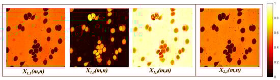
Figure 3.
Foreground module activation maps.
3.3.2. Fully Convolutional Network
The proposed FCN features a symmetric encoder–decoder architecture with pairwise layers that comprise four convolutional layers, six depthwise layers, and five resizing layers. The kernel size in the FCN is with and , and the activation function is leakyReLU. The convolution layers of the FCN are resized as follows:
Encoder
The encoder is divided into two-layer blocks that reduce background information but find different foreground features. The first block consists of two convolution layers, defined by Equation (1), followed by a max-pooling layer. The first convolution layer is , where ; there is no resizing of , which means that . The subsequent layers include another convolution operation, , followed by a max-pooling operation , which produces a feature map with dimensions of . Layer creates a feature map that reduces background information and enhances the edges of foreground features, while layer improves edges with different orientations. Figure 4 presents an example of the activation maps for and .
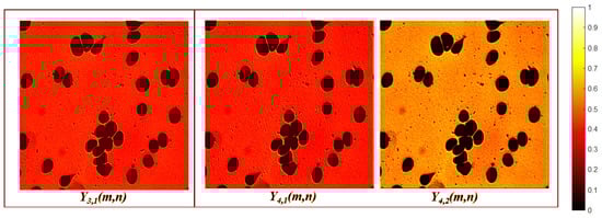
Figure 4.
First pairwise encoder layer activation maps.
The second block of encoder layers begins with a depthwise convolution, defined by Equation (3), with and no resizing (). Layer separates the foreground into two feature maps with different morphologic and gray-level patterns, as shown in Figure 5. The subsequent layers include a separable convolution, defined by Equation (4), , followed by a nearest-neighbor interpolation which generates a feature map with dimensions . The output of this block creates four feature maps, each with distinct orientations and morphological features, as shown in Figure 6.
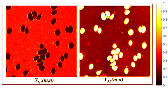
Figure 5.
Third encoder layer activation maps.
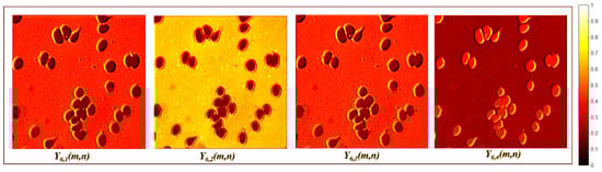
Figure 6.
Fourth encoder layer activation maps.
Bottleneck
The bottleneck suppresses the background and identifies the biological entities labeled by the GT through two convolution layers and an upsampling layer. The first bottleneck layer consists of a depthwise convolution defined by Equation (3), with no resizing (). Figure 7 shows that produces four feature maps with different orientations, morphologies, and grayscale levels. The subsequent layer includes a separable convolution , defined by Equation (4), followed by an upsampling operation which generates feature tensors with dimensions . Figure 8 illustrates how produces nine feature maps with different orientations, morphologies, and grayscale levels.
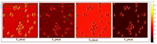
Figure 7.
First bottleneck layer activation maps.
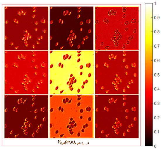
Figure 8.
Second bottleneck layer activation maps.
Decoder
The decoder utilizes the feature tensors generated in the bottleneck to produce a feature map with the same size as . The decoder is divided into two-layer blocks, which have an inverted structure compared to the encoder.
The first decoder block consists of two convolution layers followed by an upsampling operation. The first layer of this block is a depthwise convolution , defined by Equation (3), with no resizing (). The next layer is a separable convolution defined by Equation (4), followed by an upsampling operation which generates a feature map with dimensions of .
The second decoder block contains two convolution layers followed by a nearest-neighbor interpolation. The first layer in this block is a depthwise convolution , defined by Equation (3), where . The next layer is a separable convolution defined by Equation (4), followed by nearest-neighbor interpolation , producing a feature map with dimensions of .
The decoder enhances the resolution while simultaneously reducing the number of channels and eliminating irrelevant features. These irrelevant features include orientation, grayscale, and morphological patterns that are not related to the GT. This elimination is accomplished by comparing the features extracted by the encoder using the ratio of the RGB image () to the GT. As a result, two feature maps are generated that focus on foreground segmentation, as illustrated in Figure 9.
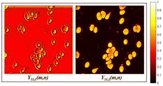
Figure 9.
Last decoder layer activation maps.
3.3.3. Output
The MBnet output segments the foreground using a pointwise convolution layer followed by a thresholding layer, which generates blobs representing the microscopic biological entities. The pointwise convolution is necessary in order to concatenate the feature maps produced by the FCN to segment the foreground, with the following expressions:
The result is shown in Figure 10. The weights computed during training are crucial for accurate segmentation. The thresholding layer separates the background from the foreground using the Otsu method [29], generating an output , as demonstrated in Figure 10. The Otsu method was selected because it has shown the ability to effectively detect biological entities in various histological and hematological studies [3].
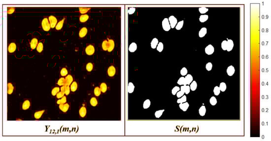
Figure 10.
Output layers.
This architecture allows MBnet to integrate color, morphological, and orientation patterns in order to separate the background and the cells or microorganisms to be segmented.
4. Datasets for Experiments
Dataset selection for segmentation and quantification experiments is a challenging step in microscopic biological entities analysis using DL because many datasets were created for very specific classification or segmentation tasks, are private, or often include processed or cropped images. For these reasons, it was necessary to select datasets meeting the following requirements:
- The datasets must contain sufficient images to train and test deep learning models effectively.
- The images should be obtained from a commercial microscope commonly used in standard laboratories.
- The raw images must be available for experimentation.
- The ground truth, or annotated masks (GT in this paper), must be designed specifically for the quantification and segmentation tasks of microscopic biological entities.
Based on these criteria, we selected the following datasets.
4.1. Blood Cell Segmentation Dataset (BBBC041Seg)
This dataset, presented in [30], contains 1328 high-resolution peripheral blood images acquired with a microscope, of which 1169 are used for training and 159 for testing. The foreground for this dataset is the blood cells. Each image has its corresponding GT, consisting of red and white blood cells, where each cell has its own GT, as shown in Figure 11. This dataset was selected to compare MBnet with other methods proposed in the literature and to perform cross-validation.
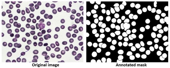
Figure 11.
BBBC041Seg image example.
4.2. Bacteria and Yeast Segmentation
The Bacteria and Yeast Complete Samples Dataset (BYCS) contains 1500 images of culture plate samples, which are microscopy-prepared media for the growth of microorganisms. The foreground for this dataset includes bacteria and yeast acquired by a microscope at 40× magnification on a fresh smear. The dataset is divided into 500 images of Staphylococcus Aaureus (SA) cultures, 500 images of Candida Albicans (CA) cultures, and 500 images of Escherichia Coli (EC) cultures. These microorganisms were selected because they represent the primary morphologies of microorganisms, namely, coccus, bacilli, and yeast-like morphologies; SA represents the coccus morphology, EC the bacillus morphology, and CA the yeast morphology. Figure 12 shows an example of each microorganism culture and their respective GTs. BYCS was selected in order to evaluate how MBnet performs in microbiological quantification and segmentation tasks involving large numbers of microorganisms within microscopic raw images.
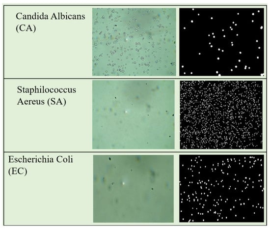
Figure 12.
BYSC dataset examples.
4.3. LeucoSet
LeukoSet is a dataset designed for the study of blood histology that was published in [31]. It comprises 1497 high-resolution images captured through a microscope. Among these, 689 images are at 40× magnification and 808 are at 100× magnification. Each image showcases a complete blood smear sample which includes erythrocytes, leukocytes, and various other components of blood tissue. The GT labels specifically identify the leukocytes, which are the foreground entities. These samples were stained using Wright’s stain, which colors the leukocyte nuclei purple. The dataset contains artifacts and exhibits significant color variations typical in clinical laboratory samples obtained under similar protocols and constraints [31].
Figure 13 presents two examples with their corresponding class labels; one image is a 40× sample displaying two lymphocytes and one basophil, while the other is a 100× sample featuring four eosinophils and one deformed leukocyte. LeukoSet was selected to explore how MBnet functions in counting and segmentation tasks involving a small number of cells (leukocytes) within a raw image that also includes cells that should not be detected, such as red blood cells.
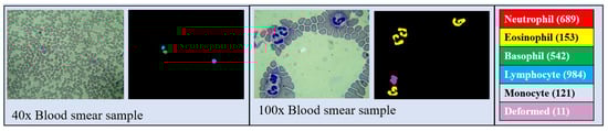
Figure 13.
LeucoSet examples.
4.4. Fluorescent Neuronal Cells v2 (FNCv2)
The FNCv2 dataset [32] was published in 2024 and contains 1874 fluorescent microscopy images with nuclei and cytoplasm of rodent neuronal cells stained with various markers to emphasize their anatomical and functional characteristics. Of these images, 750 include their corresponding GT, while the remaining images are unlabeled. Figure 14 shows an image and its respective GT. FNCv2 was selected to test MBnet with neural samples where only certain elements must be segmented and where the staining technique can change the color of the sample. The FNCv2 dataset was published recently, and several research works are utilizing it.
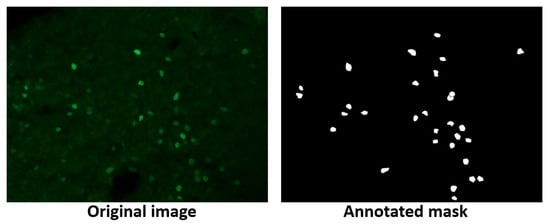
Figure 14.
FNCv2 image example.
5. Results
This section presents the results of the experiments using the datasets, the analysis of the computational cost, and a discussion.
The dataset experiments compare MBnet with different deep neural networks in different tasks related to detecting, segmenting, and counting microbiological cell entities. The BBBC041Seg experiments compare MBnet with other models referenced in the medical segmentation literature, perform a cross-validation analysis, and conduct an ablation study to assess the importance of MBnet layers. The BYSC and LeucoSet experiments evaluate the performance of MBnet against other popular networks used to count biological entities and medical segmentation. The FNCv2 experiments test MBnet in samples with different objects to be segmented and counted (nuclei and cytoplasm) and in different colors. The computational cost analysis compares the resources required to execute MBnet and other neural networks. Finally, the discussion provides an interpretation of the results of the neural networks.
The comparison metrics used in this section are categorized into performance, count, and computational cost.
5.1. Performance Metrics
The performance metrics evaluate the ability of the network to detect and segment the foreground. These metrics, as defined in [33,34], are based on the calculation of True Positives (TP), True Negatives (TN), False Positives (FP), and False Negatives (FN). The following performance metrics are used:
- Accuracy (Acc)
The ratio of correctly classified pixels to the total number of pixels in .
- F-Measure (F1)
The harmonic mean between precision and recall, measuring the overlap between the predicted blobs in and the GT blobs. In this work, F1 corresponds to the DICE coefficient, as the segmentation divides the image into foreground and background. F1 can be expressed in terms of TP, TN, FP, and FN as follows:
- Precision (P)
The ratio of TP to the total number of positives predicted in .
- Recall (R)
The ratio of TP to the total number of positives in the GT.
- Intersection over Union (IoU)
The IoU describes the extent of overlap between the bounding box of the GT blob and the bounding box of the predicted blob in . This metric is also known as the Jaccard index, and can be expressed in terms of TP, FP, and FN as follows:
5.2. Counting Metrics
The counting metrics measure the accuracy of the model in quantifying biological entities in microscopic samples. These metrics are based on the differences between the number of biological entities in the k-th GT, (), and the number of biological entities found in the k-th of the DL model , (). These metrics are derived from the sets and , where L represents the number of images (GTs or ) in the set. The counting metrics are defined as follows:
- Counting Statistic (Acm)
This statistic represents the mean and standard deviation of the absolute error defined as . When both and approach zero, it indicates that and are becoming more similar. If and approach one, it suggests that while and have similar data ranges, their statistical distributions differ. When and exceed one, there is a significant difference in both the distribution and the ranges of and .
This is the Pearson correlation coefficient between and , which measures the linear relationship between two datasets. Specifically, it assesses how many values of and are similar or identical.
- p-value
The p-value derived from the Wilcoxon hypothesis test [35] is used to evaluate the statistical differences between and . This test is appropriate because both and yield non-Gaussian distributions in every dataset. A p-value greater than 0.05 indicates that the null hypothesis () holds, meaning that and are proportional and that can be reliably used for quantification. Conversely, if the p-value is less than 0.05, the null hypothesis is rejected (), indicating statistical differences between and . Additionally, if is greater than 0.5, the statistical significance is considered marginal.
5.3. Computational Cost Metrics
The computational cost metrics evaluate the resources needed to execute a task or algorithm. The metrics chosen for this experiment are:
- Parameters
The number of parameters in the network.
- Frames per second (FPS)
The number of images that the network processes in one second.
- RAM
The average amount of RAM used to process a frame .
- Latency Inference (IT)
This metric refers to the time that a machine learning model takes to process an input and produce an output or prediction. This duration covers loading the input data, processing, and generating the final result.
- Pixels per minute (PpM)
Pixels processed by a machine learning model in one minute.
- Power
Electrical energy per second to perform the tasks of a machine learning model to load and process the input data and generate the final result.
- Inference Energy (IE)
This metric is derived from power consumption and represents the energy in Joules that a machine learning model needs to perform a single inference.
The subsequent sections outline the experiments and the results achieved using these metrics.
5.4. Experiments with BBBC041Seg Dataset
The BBBC041Seg dataset was used in [30] to evaluate different methods for blood cell segmentation using the metrics of the Jaccard index and Dice coefficient.
The evaluated methods reported in this section include classical image processing techniques such as Otsu, Balanced Histogram Thresholding (BHT), and Watershed as well as the deep neural networks of Unet, Unet++, Ternaus-Net (Ternet), Recurrent Residual Convolutional Neural Networks based on Unet (R2Unet), Attention Unet (AttNet), Attention R2Unet (AttR2Unet), a traditional FCN (FCN1), MobileNet (Mn), and ShuffleNet (Sn). Table 1 presents the segmentation results of these methods along with those of MBnet.

Table 1.
BBBC041Seg results (test set).
5.4.1. Detection and Segmentation Results Using BBBC041Seg
In terms of classical image processing methods, the BHT and Watershed methods yield the lowest results. Conversely, the Otsu method demonstrates performance comparable to the deep neural networks shown in Table 1.
In terms of deep learning models, UNet is a deep neural network with an encoder–decoder architecture. The encoder consists of convolutional layers for feature extraction, followed by downsampling layers, while the decoder includes upsampling layers followed by convolutional layers. The convolutional layers of the encoder are concatenated with the corresponding layers in the decoder. This network achieves the second-best F1 score, but a lower IoU than the other deep neural networks. According to the definitions in Equations (7) and (8), this occurs because UNet generates an inadequate representation of blood cell morphology, causing many FP and FN instances. Unet++ is an extension of Unet in which the encoder–decoder layers are connected through nested, dense, and skip pathways. This network achieves an F1 score of 88.80% and an IoU of 81.44%, indicating regular performance, likely due to a low number of TPs. TernausNet is another Unet variant, featuring an encoder based on VGG-11 pretrained on the Kaggle Carvana dataset and a decoder pretrained on ImageNet. This network delivers the best F1 score and the second-best IoU. R2Unet is a recurrent convolutional neural network with residual blocks designed to improve feature segmentation in tasks such as this one. It achieves an F1 score of 86.76% and an IoU of 77.77%, which is a moderate performance, also indicating that it is impacted by a low number of TPs. AttUnet introduces Attention Gate (AG) models to Unet to suppress irrelevant features, while AttR2Unet combines R2Unet with AGs. However, both AttUnet and AttR2Unet yield lower F1 and IoU scores than Unet and R2Unet, suggesting that AGs do not significantly contribute to cell segmentation performance. Traditional FCN (FCN1) is an encoder–decoder network designed for semantic segmentation, and uses pixelwise prediction instead of pathwise prediction. This network achieves an F1 score of 92.17% and an IoU of 75.29%, reflecting a considerable amount of FPs and FNs. MobileNet V2 (Mn) is an FCN explicitly designed for mobile devices and embedded systems, and uses depthwise separable convolutions to reduce the number of parameters and enhance inference speed [36]. Mn achieves an F1 of 87.81% and an IoU of 78.69%. This performance is attributed to its ability to effectively segment blood cells, although the results include significant noise. ShuffleNet V1 (Sn) is an efficient neural network architecture for limited recourse devices. Sn uses convolution groups and an operation to shuffle information between channels as a way of reducing computational and memory costs. The version used in this paper is an optimized version with 4061 parameters. Sn generates an F1 of 87.19% and an IoU of 78.88%, which is because the network generates errors in the morphology representation of blood cells.
MBnet achieves the highest IoU result and one of the top F1 scores at 92.17%. Based on the definitions in Equations (7) and (8) as well as the examples illustrated in Figure 15, these results indicate that MBnet effectively captures the morphology of blood cells, leading to a low number of FNs and FPs compared to TPs. However, MBnet needs help defining cell boundaries and tends to introduce noise from nonbiological objects in the sample.
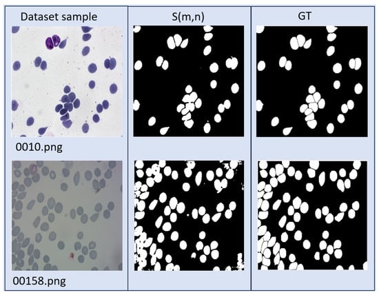
Figure 15.
Results of MBnet with two BBBC041Seg images.
The results of MBnet presented in Table 1 are supported by k-fold cross-validation with . Table 2 presents the cross-validation results, where F1 and IoU have a mean () of F1 = 92.11% and IoU = 90.91%, with a standard deviation () of 0.36 for F1 and 0.47 for IoU. The results in Table 2 suggest that the metrics of MBnet are consistent, as the range defined by includes the IoU and F1 values from Table 1. Moreover, all IoU values in Table 2 outperform the methods listed in Table 1, and all F1 scores maintain the same ranking relative to the other methods.
Table 2.
MBnet cross-validation with and IoU and F1 metrics.
5.4.2. Counting Results Using BBBC041Seg
Table 3 presents the blood cell counting metrics for BBBC041Seg. It can be observed that the of and are very similar, as . These results occur because 68% of the images have an error around 0.33, while the remaining images exhibit errors ranging from 0 to 0.6, resulting in a distribution that is skewed to the left compared to . This skewness is due to MBnet grouping several cells into a single blob, as seen in Figure 16. The other counting metrics show and a p-value of 50%, indicating proportionality between and . This result is because 68% of the number of cells and vary proportionally with an offset of 0.33, 25% of and have an offset approaching zero, and the remaining 7% exhibit errors up to 0.6.
Table 3.
MBnet counting metrics using BBBC041Seg (test set).
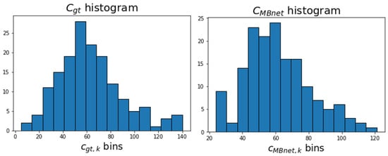
Figure 16.
Histograms of and .
5.4.3. Ablation Experiments
An ablation study was conducted to assess the significance of the different MBnet layers. This study comprised five experiments: one in which the foreground module was removed, three where specific blocks of the FCN were omitted, and one where the pointwise convolution was excluded. The selection of the layers to be ablated was based on preserving the symmetry and dimensionality of the image. The variations in the MBnet architecture resulting from these five ablation experiments are illustrated in Figure 17, and are described as follows:
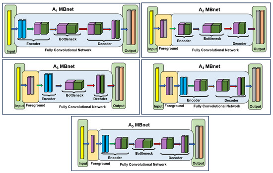
Figure 17.
Ablation architecture.
This version has an architecture consisting of 538 parameters, and does not include the foreground module. In this case, the input is fed into the FCN, which generates an output with lower performance compared to MBnet. This reduced performance is because the variance among the RGB channels is significantly lower than the information provided by the foreground module.
This version of the architecture has 218 parameters, but eliminates the first encoder block and second decoder block. Consequently, the network generates fewer morphological foreground features than MBnet, leading to lower performance.
This architecture version has 151 parameters, but eliminates the second encoder block and first decoder block. Consequently, neither orientation nor morphological foreground features are generated, leading to lower performance than MBnet.
This architecture version has 339 parameters, but the bottleneck is eliminated; as a result, the network does not generate orientation foreground features, leading to lower performance than MBnet.
This version of the architecture has 572 parameters and does not include the pointwise convolution for the foreground. The three channels are passed directly into the first encoder block in this configuration; however, a problem arises because some activations from the layer inhibit the background, while others inhibit the foreground. As these activations enter the first block of the encoder, they tend to cancel each other out, resulting in lower performance of compared to the original model. This experiment highlights the importance of feature weighting via the pointwise convolution weights.
Additional ablation experiments were developed to consider the removal of other layers and replace the BFCE function with cross-entropy; however, these did not produce successful segmentation results.
Figure 18 shows the generated by the ablation experiments with the image 00158.png. Table 4 presents the average results of the ablation study in terms of F1, IoU, Acm, , and p-value. The F1 and IoU results in the five ablation experiments are lower than those achieved by the original MBnet architecture. These results indicate that removing layers from MBnet negatively affects its detection and segmentation capabilities. Regarding the Acm, , and p-value, the results reveal that removing layers generates a less accurate count of microscopic biological entities compared to the original version of MBnet. Furthermore, based on the p-value, the five ablation experiments generate statistically significant differences between and . In contrast, as shown in Table 3, the original MBnet architecture does not show a statistical difference between and , further emphasizing the robustness of the original model compared to the ablation experiments.
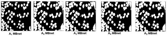
Figure 18.
Example of ablation experiments with image 00158.png from the BBBC041Seg test set.
Table 4.
Ablation results using BBBC041Seg (test set).
5.5. Experiments with BYSC Dataset
These experiments involve training and testing MBnet and other deep neural networks widely recognized in the literature for detecting and quantifying bacteria and yeast. The neural networks chosen for these experiments are well known for their applications in counting analysis and medical segmentation. Additionally, we selected a popular recurrent neural network and a transformer-based network for our study. The networks utilized in this experiment include:
- ResNet-50 (Rn)
Introduced in 2015, this network consists of 50 layers and includes residual blocks with shortcut connections, which help to maintain gradient flow during training and mitigate the vanishing gradient problem [36]. The autoencoder version of ResNet-50 is commonly used for segmentation tasks due to its ability to maintain stable gradient flow even in the decoder, making it easier to train deep networks. Its depth also supports transfer learning, while using residual blocks enhances its generalization capacity compared to other CNN architectures.
- Base UNet (Unt)
This is the base UNet network tested in the review of [37], except trained with the BYSC dataset.
- Long Short-Term Memory (Lstm)
This network is an autoencoder with a recurrent LSTM module, as used in [38]. The autoencoder includes four convolutional layers, defined by Equation (1), with kernels and two max-pooling layers. The bottleneck is the LSTM module, and the decoder consists of four convolutional layers, also defined by Equation (1), with kernels and two upsampling layers.
- Transformer (Tnet)
This is an autoencoder with a transformer module, as described in [39]. It shares the same encoder and decoder structure as the LSTM autoencoder, but the bottleneck consists of a transformer with two layers.
- MobileNet V2 (Mn) and ShuffleNet V1 (Sn)
In addition to the aforementioned networks, MobileNet and ShuffleNet are included in the analysis with the BYSC dataset to compare MBnet against other efficient networks designed explicitly for resource-limited devices.
5.5.1. Detection and Segmentation Results Using BYSC
Table 5 reports the results of the BYSC testing experiments, and Figure 19 and Figure 20 present a processing example of all the networks.
Table 5.
BYSC performance (test set).
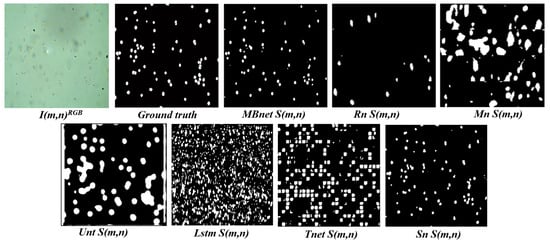
Figure 19.
Example of segmentation results from a BYSC dataset image.
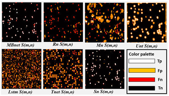
Figure 20.
Analysis of the segmentation results with BYSC.
All networks achieve good accuracy, as they are able to detect the background properly and most of the pixels in the images belong to the background; however, due to the significant imbalance between the number of background and foreground pixels, good performance in background detection does not necessarily imply good performance in foreground detection. Foreground detection and segmentation are assessed using the F1 and IoU metrics. Regarding these metrics, Rn fails to segment the bacteria and yeast in , as shown in Figure 19 and Figure 20. This failure results in a TP count close to zero, while the numbers of FN and FP instances are high, causing values close to zero in IoU, P, R, and F1. Mn poorly segments the bacteria and yeast, leading to a low number of TPs and high FPs and FNs, as shown in Figure 20. As a result, the values of IoU, P, R, and F1 resulting from of Mn are very low. Unt performs regular segmentation of the bacteria and yeast, producing a moderate number of TPs but a high number of FPs and FNs, as seen in Figure 20. Consequently, its IoU, P, R, and F1 metrics are moderate. Lstm segments some microorganisms, but introduces much noise in , leading to moderate values for R and near-zero values for F1, P, and IoU. Tnet detects and counts the microorganisms, but contains significant noise. The segmentation does not accurately follow the morphology of the microorganisms, resulting in low values in P, F1, and IoU and moderate values in R. This can be observed in Figure 19, where microorganisms are detected but a significant number of FPs and FNs are also present. Sn correctly segments bacteria and yeast in , achieving the second-best results in F1, P, R, and IoU. These results are because Sn manages to detect and segment microorganisms. However, Sn merges blobs, generating some errors in the morphology representation and resulting in many FPs. These results can be seen in Figure 20, where Sn performs well in segmentation but some blobs that are too close together are merged.
MBnet successfully segments the bacteria and yeast in , achieving the best F1, P, R, and IoU results. These results are because MBnet generates a high number of TPs and a low number of FPs and FNs, as seen in Figure 20. However, the IoU metric has a moderate average because the blobs generated by MBnet to represent the microorganisms are smaller in area than the blobs in the GT, resulting in some FNs, as shown in Figure 20.
5.5.2. Counting Results Using BYSC
Figure 21 shows a bar graph of the mean () and standard deviation () for the and sets, where MBnet and Sn demonstrate remarkable statistical similarity compared to the other networks. Additionally, demonstrates a closer similarity to than .
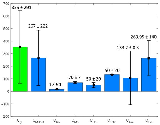
Figure 21.
Bar graph of and with BYSC.
Table 6 displays the counting metrics for the BYSC dataset divided by the subset classes CA, EC, and SA. According to the results from the BYSC dataset, MBnet achieves better and metrics than the other networks. The metric for and , indicating low error values and close to one, demonstrates strong linear correlation between and . However, the p-value is zero, suggesting that and have marginal statistical significance. These results occur because MBnet generates counting results similar to in the CA and SA classes and proportional in the EC class, as seen in Figure 22, where is represented by the brown line and by the magenta line. The CA, EC, and SA subsets have values close to one, with the SA class exhibiting the highest . Regarding , all three subsets have values less than one, with the CA subset reporting the lowest . Regarding the p-value, it is greater than 5% for the CA and SA classes, while it is zero for the EC class. These results confirm that is significantly similar to for the CA and SA classes. On the other hand, shows marginal statistical significance but remains proportional to in the EC subset, with .
Table 6.
BYSC dataset counting results (test set).
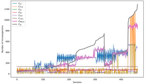
Figure 22.
Counting results with BYSC dataset.
Mn presents with values ranging from 61 to 78, generating an , a close to 0.5 and a p-value of zero for the entire dataset and classes. These metrics suggest that Mn detects the microorganisms with marginal statistical differences regarding but produces too large of blobs, causing them to merge and leading to errors in detection, counting, and segmentation.
Unt produces a with values ranging from 20 to 80, resulting in . The is close to zero for the EC and SA classes and 0.38 for the CA class, while the p-value is zero for the entire dataset. These metrics together with Figure 22 indicate that Unt performs well in counting samples with few microorganisms, such as some samples in the CA class, but fails to detect large quantities of microorganisms, as found in the EC and SA samples.
Lstm reports with values ranging from 132 to 135, generating . The values are close to zero or negative, and the p-value is zero for the entire dataset and class subsets. Figure 22 shows that these metrics arise because Lstm produces nearly constant results across all dataset images, which differ significantly from the values of the GTs.
Tnet has , with a value of 0.54 for the entire dataset, 0.54 for the CA class, −0.02 for the EC class, and 0.58 for the SA class. However, the p-value is zero for the dataset and all classes. Figure 22 shows that these metrics are due to a statistical difference between and in the EC class, but the difference is marginal in the CA and SA classes.
Sn has similar to MBnet, and is the second closest to . According to Table 6, the Acm values for the database and the CA, EC, and SA classes are close to zero. The values in the database and the classes are near one, indicating a linear relationship between and . However, the p-values reveal statistical differences between the CA, EC, and SA classes and the dataset. Consequently, while Sn has a similar to , there are notable statistical differences between them, leading to a similarity below that of .
5.6. Experiments with LeucoSet
5.6.1. Detection and Segmentation Results with LeucoSet
The experiments with this dataset involved basic learning, retraining, and transfer learning to segment leukocytes from blood smear samples.
The basic learning experiment involved training Rn, Mn, Unt, Lstm, Tnet, Sn, and MBnet using 2807 LeucoSet training images throughout 100 epochs. The results are presented in Table 7. MBnet achieved an accuracy (Acc) of 100% with the training set and 99.6% with the testing dataset, while the other networks achieved an accuracy of 98% with both the training and testing datasets. Regarding the other performance metrics, MBnet showed better F1, P, R, and IoU averages compared to the other networks, though with higher standard deviations. The mean values of F1 and IoU for MBnet indicate that the blobs in detect the leukocytes but fail to accurately represent their morphology, as shown in Figure 23. The standard deviation of F1 and IoU suggests that the morphological representation of leukocytes varies across different , likely because MBnet divides each leukocyte into multiple blobs, leading to a significant number of FN and FP instances. In contrast, the Rn, Mn, Unt, Lstm, and Tnet networks exhibit average F1 and IoU values close to zero, as they are ineffective in detecting and segmenting leukocytes. Finally, Sn achieves an accuracy (Acc) of 94.65% with the testing dataset. Regarding the other performance metrics, Sn achieves the second-best F1, P, R, and IoU averages compared to MBnet and the other networks. However, the standard deviations of these metrics are high. These results indicate that the blobs in detect the leukocytes but fail to accurately represent their morphology.
Table 7.
LeucoSet performance during the basic learning experiment (test set).
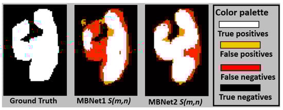
Figure 23.
Leukocyte segmentation example.
The retraining experiment used the parameters obtained from the BYSC training as the initial conditions. Following this, the networks were trained with LeucoSet for 100 epochs. This experiment yielded the best results when using LeucoSet, which are are presented in Table 8. MBnet achieves the best average results, but its F1, P, R, and IoU values exhibit high standard deviations. The mean F1 and IoU indicate that the blobs in detect the leukocytes and can correctly represent their morphology, as shown in Figure 23; however, the high standard deviation in F1 and IoU suggests that MBnet has difficulties defining the perimeter of the leukocytes, resulting in some FPs and FNs. Rn, Mn, and Unt achieve good accuracy, as these networks effectively detect the background. However, they fail to identify leukocytes, resulting in numerous irrelevant blobs and lower F1, P, R, and IoU scores. The Lstm model demonstrates moderate Acc and R but shows poor F1, P, and IoU averages because it primarily detects noise. Tnet successfully detects and counts leukocytes but fails to segment their morphology, leading to low P, R, F1, and IoU scores. Finally, Sn achieves an accuracy (Acc) of 98.38% with the testing dataset. Regarding other performance metrics, Sn achieves the second-best F1, P, R, and IoU averages. The mean and standard deviation of F1 and IoU indicate that the blobs in detect the leukocytes and can correctly represent their morphology. However, these results remain below the performance of MBnet.
Table 8.
LeucoSet performance during the retraining experiment (test set).
The transfer learning experiment used parameters obtained from training on the BYSC dataset. In this process, 25% of the network layers were frozen, then the model was trained using the LeucoSet dataset for 100 epochs. The networks all show an average accuracy below 90%, as freezing the layers limits their ability to learn new background and foreground features from the LeucoSet images. The results indicate that the F1, P, R, and IoU averages are close to zero for all the networks, as they primarily detect and segment erythrocytes, resulting in a high number of FPs. Additionally, the networks generate many FNs, as they need help learning the background color features in the LeucoSet images.
5.6.2. Counting Results Using LeucoSet
The leukocyte counting experiment was conducted using MBnet trained with basic learning (referred to as MBnet1), MBnet that was retrained (referred to as MBnet2), and the retrained configurations of the Rn, Mn, Unt, Lstm, and Tnet networks. Other basic learning and transfer learning experiments were excluded from the counting analysis because they reported F1, P, R, and IoU values close to zero, rendering it impossible to count leukocytes accurately.
Figure 24 presents the bar graph of the and sets. MBnet demonstrates the highest statistical similarity with the GT values in this comparison. Table 9 details the counting metrics obtained using LeucoSet. MBnet1 detects leukocytes but generates multiple blobs per leukocyte, leading to counting discrepancies between and . These discrepancies result in an in , a of 0.22, and a p-value of zero, indicating statistical differences between of MBnet1 and . MBnet2 successfully detects and segments leukocytes, generating a single blob to represent each leukocyte in lymphocytes, basophils, and monocytes. However, MBnet2 occasionally fails with eosinophils and multinucleated neutrophils, segmenting them with multiple blobs, which causes a slightly greater than . These results of MBnet2 produce the best Acm in the LeucoSet experiments, a of 0.77, and a p-value of zero, suggesting marginal statistical differences.
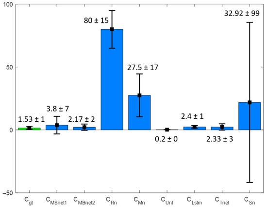
Figure 24.
Bar graph of and with LeucoSet.
Table 9.
LeucoSet counting results (test set).
Rn produces numerous blobs in regions with accumulated erythrocytes, resulting in an in and a close to zero due to the lack of correlation between and . Additionally, the p-value is zero, suggesting that the observed statistical differences stem from misinterpreting erythrocytes as part of the foreground.
Mn produces numerous blobs in regions with erythrocytes and leukocytes, causing an , a close to zero, and a p-value of zero. These results reflect statistical differences due to the lack of correlation between and .
Unt fails to produce blobs that accurately represent leukocytes. This is evident from the fact that the mean and standard deviation () of is nearly zero, resulting in an accuracy measurement of . Additionally, is zero, and the p-value is also zero. These findings indicate statistically significant differences, as Unt cannot detect leukocytes.
Lstm creates two or three clusters in areas with grouped erythrocytes, resulting in an , a , and a p-value of zero. This indicates statistical differences, as these clusters do not correspond to leukocytes.
Tnet achieves the second-best mean for because it is the second closest to ; however, the values and the p-value indicate statistical differences. Figure 25 shows that Tnet successfully detects leukocytes but also generates noise, contributing to the statistical significance compared to the GT.
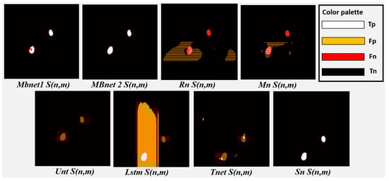
Figure 25.
Analysis of the segmentation results using LeucoSet.
Sn has regular results in terms of Acm, and the and the p-value shows statistical differences. However, good results in Sn segmentation are observed in Figure 25 and Figure 26. These results are because Sn performs well in 67% of the blood samples, where it segments leukocytes, but has inferior results in the rest, as it segments both leukocytes and erythrocytes. The huge differences between these results generate a and a very high , which can be seen in Figure 24.
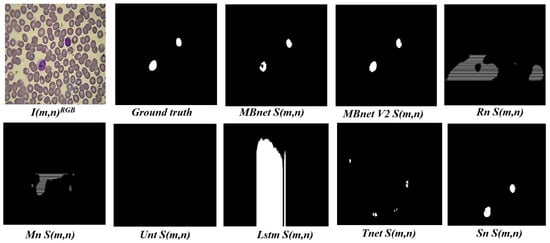
Figure 26.
Example of segmentation results from LeucoSet image.
5.7. Experiments with FNCv2
The experiments with FNCv2 are focused on comparing the performance of MBnet against other methods that have utilized this dataset, as published in [32,40,41]. These methods are variations of the UNet and YOLO networks. Table 10 displays the results of these networks alongside MBnet with basic learning (MBnet1) and MBnet with retraining (MBnet2).
Table 10.
FNCv2 performance results (test set).
Table 10 shows that each author trained and tested their models differently when using this dataset. The authors of [32] developed a model called ResUNET, which achieved good results but was specifically trained based on the fluorescence color of the samples. The methods presented in [40] are UNet methods, with average and dispersion values reported for the F1, P, and R metrics. The approaches in [41] also generated good results, but were trained according to the spatial resolution of the input, as outlined in Table 10.
MBnet1 was initially trained using 70% of all images in the dataset, resulting in very low performance, as shown in Table 10. However, a subsequent experiment utilized a different approach; the model was first trained on grayscale images for 100 epochs, then retrained on color images for another 100 epochs, leading to an improved performance. Table 10 indicates that the results of MBnet2 are comparable to those of YOLO. However, MBnet2 is invariant to the spatial resolution of the input images. Figure 27 shows an example of segmentation for each sample of different staining colors.
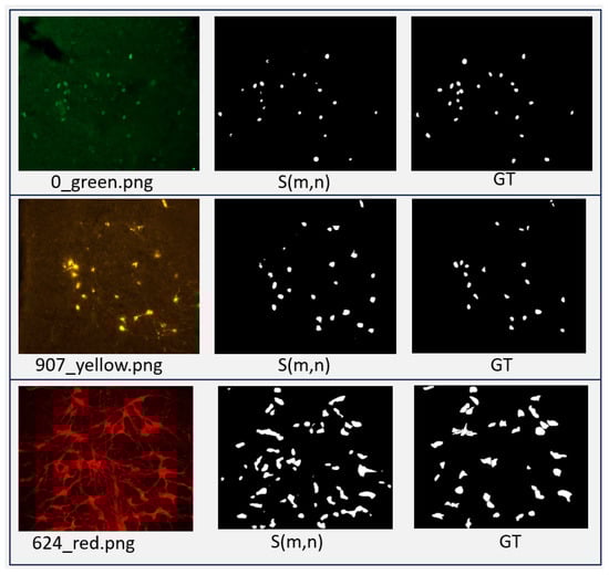
Figure 27.
Segmentation results of MBnet on samples stained with different colors.
MBnet1 reports a lower F1 score compared to the UNet networks from [40] and the YOLO networks from [41]. Its counting metrics were , , and p-value = 0. These results suggest that MBnet1 successfully detects the foreground but does not accurately define the nuclei and cytoplasm morphology. In contrast, MBnet2 achieves an F1 score comparable to the YOLO results from [41], with counting metrics of , , and p-value=0. These results suggest that MBnet2 effectively detects and follows the morphology of nuclei and cytoplasm. Errors occur only when overlapping cells generate merged blobs.
5.8. Computational Cost Analysis
The training experiments were conducted on a Dell Workstation, while the testing experiments were performed using both the workstation and a GPU-embedded system. The workstation had an Intel Xeon CPU processor, 9 GB of RAM, and Python 3.9. In contrast, the GPU-embedded system consisted of an NVIDIA Jetson TX2, which features a Dual-Core NVIDIA Denver 2 64-bit CPU, a Quad-Core ARM Cortex-A57 MPCore, 8 GB of RAM, and operates with Python 3.6. It also supports the Open Neural Network Exchange (ONNX) standard.
This computational cost analysis evaluates the composition of deep neural networks, processing speed, and energy consumption.
5.8.1. Composition of the Deep Neural Networks
Table 11 compares the MBnet architecture with the other deep neural network architectures used in the experiments. This comparison highlights the number of convolutional, dense, and recurrent layers as well as the number of neurons in each model. The Rn and Sn models both contain 49 convolutional layers, although Rn has a significantly higher total of convolutional neurons. The Mn model has 60 convolutional layers with 2,602,792 neurons and no dense or recurrent layers. The Tnet model comprises six convolutional layers and four dense layers, featuring 2,882,304 convolutional neurons and 1,536 dense neurons. The Lstm model contains no convolutional layers but has two recurrent layers with 256 neurons each and one dense layer with 1200 neurons. The UNet architecture and its TernausNet, UNet++, and R2UNet variants are all based on convolutional designs lacking any dense or recurrent components. Among these, Unt is the most complex, incorporating 23 convolutional layers and 153,490,960 convolutional neurons, TernausNet follows with 18 layers and 123,899,904 neurons, R2UNet has 22 layers and 43,147,392 neurons, and UNet++ includes 40 layers and 9,327,936 neurons. Each of these networks utilizes kernels of varying sizes. In contrast, MBnet is significantly less complex than all these networks, featuring just 63 convolutional neurons distributed across 12 layers, all using a 3 × 3 kernel size.
Table 11.
Number of layers and neurons of the deep neural networks.
5.8.2. Processing Speed and Energy Consumption
Table 12 shows that MBnet has a significantly lower computational cost than other networks, primarily due to its smaller number of parameters, resulting in a more compact design.
Table 12.
Computational cost metrics.
In terms of FPS and IT, all networks provide instantaneous responses for each image , but MBnet achieves the best performance. Regarding RAM usage, MBnet consumes hundreds of times less memory than the other methods, leading to a negligible load on both the Jetson and the workstation. In contrast, Rn and Mn place a substantial RAM burden on these systems. Furthermore, in terms of pixels processed per minute (PpM), MBnet can handle more pixels per minute, processing around 6318 images in 60 s. This capability indicates that MBnet can consistently process a higher volume of images over an extended period than other networks. Regarding energy consumption, MBnet uses 0.5 Watts and 0.63 mJ for each processed image. These results demonstrate that MBnet can process over 900 images with only 0.5 Joules, consuming less energy per inference than the other networks.
5.9. Discussion
According to Section 5.4, Section 5.5 and Section 5.6, MBnet demonstrates superior performance in detection, counting, and segmentation across all of the datasets utilized in this research. This indicates that the architecture of MBnet possesses the necessary structure and parameters for the effective segmentation of cells and microorganisms.
The architecture includes a foreground module, an FCN, and an output module. The foreground module consists of 37 parameters that enhance the detection of foreground features. The encoder of the FCN has 101 parameters dedicated to extracting orientation and morphological features. The bottleneck contains 121 parameters that generate the segmentation feature maps. The remaining 316 parameters are part of the encoder and output layers, which weigh the results to produce the final binary segmentation. The architecture of MBnet effectively generates the right features for segmentation. However, removing layers from the foreground module or FCN reduces performance.
The MBnet design effectively segments blood cells in the BBBC041Seg dataset, and can accurately detect and counts microorganisms in the BYSC dataset. In the LeucoSet results, MBnet can learn to segment leukocyte nuclei with basic training, and to segment entire leukocytes after retraining. In the FNCv2 results, MBnet detects the nuclei and cytoplasm, but cannot capture their morphology with basic learning. However, its segmentation results improve significantly when a retraining strategy is applied. According to the results with all datasets, MBnet integrates color, orientation, and morphological features to generate a binary segmentation based on the analyzed activation maps. The supervised training and retraining also help to understand various visual contexts related to the background and foreground in microscopic samples.
ResNet has 55 million parameters, which corresponds to a factor of 96,680 times more parameters than MBnet, yet its IoU, F1, and results are close to zero on the BYSC and LeucoSet datasets. These results are because its many layers and parameters generate high computational costs, overfitting problems, and unnecessary features, as the features required to represent microorganisms and cells do not justify the large number of parameters.
MobileNet has 22 million parameters, or 38,756 times more than MBnet, and its IoU, F1, and averages on BYSC and LeucoSet are moderate. Our analysis suggests that the MobileNet architecture has receptive fields of different sizes that generate features describing microorganisms and cells along with a significant amount of noise, resulting in many FPs.
Unet has 34 million parameters, equivalent to 60,023 times the parameters of MBnet. Unet shows moderate IoU, F1, and on BYSC; while it detects microorganisms, its excess parameters introduce substantial noise when reconstructing the foreground morphology, generating many FPs. On LeucoSet, the results are close to zero because Unet’s learning is affected by gradient vanishing.
Lstm has 7 million parameters, or 12,537 times more parameters than MBnet. This network reports moderate IoU, F1, and on BYSC and zero on LeucoSet, as LSTM fails to understand the spatial relationships of microorganisms and cell morphology.
Tnet has 40 times more parameters than MBnet and its IoU and F1 scores are low on BYSC and LeucoSet, which is because the number of training images in these datasets is insufficient to train the transformer. Additionally, according to our experiments, the number of heads and the size of the feedforward network need to be increased in order to capture the necessary foreground features.
Sn has 4061 parameters, and its segmentation performance can generate blobs that effectively detect and represent microscopic biological entities. In terms of counting, Sn demonstrates comparable results to MBnet on BYSC and average results on LeucoSet. Our analysis shows that Sn has the second-best performance and second-lowest computational cost, surpassed only by MBnet. This suggests that fewer parameters may be linked to improved performance.
6. Conclusions
This paper presents the Extreme-Lightweight Neural Network for Microbiological and Cell Analysis model (MBnet), which is designed to operate with significantly lower computational cost than existing models. MBnet consists of only 575 trained parameters and can be used for detecting and counting microbiological entities in microscopic samples. Experiments were carried out using several datasets: BBBC041Seg for blood cell segmentation, BYCS for bacteria and yeast segmentation, LeucoSet for leukocyte segmentation, and FNC for nuclei and cytoplasm segmentation.
BBBC041Seg has 1328 peripheral blood images along with their respective GTs, which are used to segment blood cells. MBnet generates blobs that adequately represent the morphology of blood cells, achieving the best IoU of 90.98% and one of the best F1 scores with 92.17%. However, MBnet sometimes creates a single blob to represent cells that are clustered together, leading to some errors in cell counting. Despite this error, the p-value and results indicate that is proportional to the of BBBC041Seg.
The BYSD dataset contains a database of 500 images of CA culture plates, 500 images of EC, and 500 images of SA. MBnet achieves better results than other methods in detecting and counting microorganisms. According to the p-value and results, is proportional to for the CA and SA classes. For the EC class, exhibits marginal statistical differences relative to . However, the other neural networks fail to correctly detect the microorganisms in this dataset, generating significant statistical differences between the counts of these networks and .
LeucoSet comprises 5000 smear blood images containing blood cells and background along with annotated masks developed to detect, quantify, and classify leukocytes. MBnet was able to detect and segment the leukocyte nuclei in the basic learning experiment by using the features that distinguish leukocytes from erythrocytes. However, because granulocytes may have multiple nuclei, a statistical difference is observed between and . In the retraining experiment, MBnet could successfully detect and segment leukocytes, although it occasionally fails in cases where it generated multiple regions to represent multinucleated eosinophils and neutrophils, resulting in a marginal statistical difference between and .
FNCv2 consists of 750 fluorescent microscopy images with nuclei and cytoplasm of rodent neuronal cells stained with markers of various colors. During initial training, MBnet detects the nuclei and cytoplasm but cannot follow their morphology. In subsequent retraining experiments, MBnet shows improved segmentation and counting results. This improvement occurs because the network learns color features more effectively during retraining after learning the orientation and color features.
Together with the results of the cross-validation and ablation studies, the experiments developed to evaluate MBnet’s segmentation and counting abilities across the four datasets indicate that the MBnet architecture and its learning algorithm are effective for binary segmentation tasks involving cells and microorganisms. This is illustrated by the fact that MBnet outperformed all deep neural networks in detection, counting, and segmentation tasks throughout our experiments. However, MBnet does have some disadvantages. One of these is that it sometimes struggles to accurately define the perimeters of microorganisms and cells, leading to situations in which a single blob may represent multiple organisms. Additionally, MBnet can produce oversegmentation in cells that contain multiple nuclei. Despite these issues, metrics such as F1, IoU, p-value, and indicate that MBnet is well suited for detecting and counting biological entities in microscope image samples, particularly in histological, hematological, and microbiological applications. With regard to computational cost, the architecture of MBnet comprises 12 layers and 63 convolutional networks with a kernel size of , generating a significantly lower computational cost than the other networks analyzed in our experiments. This is evident in the computational cost metrics, where MBnet demonstrates significantly better inference times, image processing per minute, and energy consumption than the other networks.
According to our deep neural network experiments, ShuffleNet (Sn) is the second-best model in terms of computational cost, number of parameters, detection, counting, and segmentation, while the rest of the networks have lower performance as the complexity of their architectures increases. These results suggest that a more compact model with a better-organized architecture will have better results in segmenting and counting microscopic biological entities.
The evidence presented in this research demonstrates that MBnet is an effective model for detection and quantification tasks related to the analysis of cells and microorganisms. Future work will focus on integrating MBnet into an Application Programming Interface (API) for bioinformatics applications, telemedicine, clinical analysis, and medical diagnosis.
Author Contributions
J.A.R.-Q. provided funding acquisition and supervision; E.A.S.-G. and J.A.R.-Q. proposed the methodology, formal analysis, and original draft; M.I.C.-M. provided recourse, review, and editing; C.A.-Q. provided conceptualization and data curation. All authors have read and agreed to the published version of the manuscript.
Funding
This research was funded by Tecnologico Nacional de Mexico grant number 19182.24-P.
Institutional Review Board Statement
Not applicable.
Informed Consent Statement
Not applicable.
Data Availability Statement
The authors will provide the BYSC dataset and MBnet source file upon request. For additional information, please visit https://github.com/pertmdcie/NEUROBL and refer to the README file.
Acknowledgments
The authors express their gratitude for the support received in various areas from Tecnologico Nacional de Mexico/I.T. Chihuahua and Faculty of Medicine and Biomedical Sciences of Universidad Autonoma de Chihuahua.
Conflicts of Interest
The authors declare no conflicts of interest.
References
- Rani, P.; Kotwal, S.; Manhas, J.; Sharma, V.; Sharma, S. Machine Learning and Deep Learning Based Computational Approaches in Automatic Microorganisms Image Recognition: Methodologies, Challenges, and Developments. Arch. Comput. Methods Eng. 2022, 29, 1801–1837. [Google Scholar] [CrossRef]
- Zhang, Y.; Jiang, H.; Ye, T.; Juhas, M. Deep Learning for Imaging and Detection of Microorganisms. Trends Microbiol. 2021, 29, 569–572. [Google Scholar] [CrossRef] [PubMed]
- Zhang, J.; Li, C.; Rahaman, M.; Yao, Y.; Ma, P.; Zhang, J.; Zhao, X.; Jiang, T.; Grzegorzek, M. A comprehensive review of image analysis methods for microorganism counting: From classical image processing to deep learning approaches. Artif. Intell. Rev. 2022, 55, 2875–2944. [Google Scholar] [CrossRef] [PubMed]
- Ma, P.; Li, C.; Rahaman, M.; Yao, Y.; Zhang, J.; Zou, S.; Zhao, X.; Grzegorzek, M. A state-of-the-art survey of object detection techniques in microorganism image analysis: From classical methods to deep learning approaches. Artif. Intell. Rev. 2023, 56, 1627–1698. [Google Scholar] [CrossRef] [PubMed]
- Rayed, M.E.; Islam, S.M.S.; Niha, S.I.; Jim, J.R.; Kabir, M.M.; Mridha, M.F. Deep learning for medical image segmentation: State-of-the-art advancements and challenges. Inform. Med. Unlocked 2024, 47, 101504. [Google Scholar] [CrossRef]
- Wu, Y.; Gadsden, A. Machine learning algorithms in microbial classification: A comparative analysis. Front. Artif. Intell. 2023, 6, 1200994. [Google Scholar] [CrossRef]
- Gaikwad, D.; Mahale, V.; Gaikwad, A. A Review on Blood Disease Detection using Artificial Intelligence Techniques. In Proceedings of the 2024 IEEE International Conference on Big Data and Machine Learning (ICBDML), Bhopal, India, 24–25 February 2024; pp. 21–26. [Google Scholar]
- Shahzad, M.; Ali, F.; Shirazi, S.H.; Rasheed, A.; Ahmad, A.; Shah, B.; Kwak, D. Blood cell image segmentation and classification: A systematic review. Peer J Comput. Sci. 2024, 10, e1813. [Google Scholar] [CrossRef]
- Park, B.; Shin, T.; Kang, R.; Fong, A.; McDonogh, B.; Yoon, S.-C. Automated segmentation of foodborne bacteria from chicken rinse with hyperspectral microscope imaging and deep learning methods. Comput. Electron. Agric. 2023, 208, 107802. [Google Scholar] [CrossRef]
- Ferrari, A.; Lombardi, S.; Signoroni, A. Bacterial colony counting with Convolutional Neural Networks in Digital Microbiology Imaging. Pattern Recognit. 2017, 61, 629–640. [Google Scholar] [CrossRef]
- Sun, B.; Wang, Z.; Lin, J.; Chen, C.; Zheng, G.; Yue, S.; Wang, H.; Kang, X.; Chen, X.; Hong, W.; et al. Automatic quantitative analysis of metabolism inactivation concentration in single bacterium using stimulated Raman scattering microscopy with deep learning image segmentation. Med. Nov. Technol. Devices 2022, 14, 100114. [Google Scholar] [CrossRef]
- Zou, H.; Sopasakis, A.; Maillard, F.; Karlsson, E.; Duljas, J.; Silwer, S.; Ohlsson, P.; Hammer, E.C. Bacterial community characterization by deep learning aided image analysis in soil chips. Ecol. Inform. 2024, 81, 102562. [Google Scholar] [CrossRef]
- Kanchanapiboon, P.; Songsaksuppachok, C.; Chusorn, P.; Ritthipravat, P. Speed meets accuracy: Advanced deep learning for efficient Orientia tsutsugamushi bacteria assessment in RNAi screening. Intell. Syst. Appl. 2024, 22, 200356. [Google Scholar] [CrossRef]
- Prangemeier, T.; Wildner, C.; Françani, A.O.; Reich, C.; Koeppl, H. Yeast cell segmentation in microstructured environments with deep learning. Biosystems 2022, 211, 104557. [Google Scholar] [CrossRef] [PubMed]
- Ghafari, M.; Clark, J.; Guo, H.-B.; Yu, R.; Sun, Y.; Dang, W.; Qin, H. Complementary performances of convolutional and capsule neural networks on classifying microfluidic images of dividing yeast cells. PLoS ONE 2021, 16, e0246988. [Google Scholar] [CrossRef] [PubMed]
- Hung, J.; Goodman, A.; Ravel, D.; Lopes, S.C.P.; Rangel, G.W.; Nery, O.A.; Malleret, B.; Nosten, F.; Lacerda, M.V.G.; Ferreira, M.U.; et al. Keras R-CNN: Library for cell detection in biological images using deep neural networks. BMC Bioinform. 2020, 21, 300. [Google Scholar] [CrossRef]
- Katharina, P.; István, K.; János, T. An automated neural network-based stage-specific malaria detection software using dimension reduction: The malaria microscopy classifier. MethodsX 2023, 10, 102189. [Google Scholar] [CrossRef]
- Maity, M.; Jaiswal, A.; Gantait, K.; Chatterjee, J.; Mukherjee, A. Quantification of malaria parasitaemia using trainable semantic segmentation and capsnet. Pattern Recognit. Lett. 2020, 138, 88–94. [Google Scholar] [CrossRef]
- Libouga, I.O.; Bitjoka, L.; Li Gwet, D.L.; Boukar, O.; Njan Nlôga, A.M. A supervised U-Net based color image semantic segmentation for detection and classification of human intestinal parasites. E-Prime Adv. Electr. Eng. Electron. Energy 2022, 2, 100069. [Google Scholar] [CrossRef]
- Halima, I.; Maleki, M.; Frossard, G.; Thomann, C.; Courtial, E.-J. Accurate detection of cell deformability tracking in hydrodynamic flow by coupling unsupervised and supervised learning. Mach. Learn. Appl. 2024, 16, 100538. [Google Scholar] [CrossRef]
- Arora, P.; Tewary, S.; Krishnamurthi, S.; Kumari, N. An experimental setup and segmentation method for CFU counting on agar plate for the assessment of drinking water. J. Microbiol. Methods 2023, 214, 106829. [Google Scholar] [CrossRef] [PubMed]
- Arora, P.; Tewary, S.; Krishnamurthi, S.; Kumari, N. Impact of Training Data, Ground Truth and Shape Variability in the Deep Learning-Based Semantic Segmentation of HeLa Cells Observed with Electron Microscopy. J. Imaging 2023, 9, 59. [Google Scholar] [CrossRef] [PubMed]
- Ali, M.A.S.; Misko, O.; Salumaa, S.-O.; Papkov, M.; Palo, K.; Fishman, D.; Parts, L. Evaluating Very Deep Convolutional Neural Networks for Nucleus Segmentation from Brightfield Cell Microscopy Images. SLAS Discov. 2021, 26, 1125–1137. [Google Scholar] [CrossRef] [PubMed]
- Hajji, M.; Benhala, B.; Hamdi, I. Survey of Gradient Descent Variants and Evaluation Criteria. In Proceedings of the 2024 4th International Conference on Innovative Research in Applied Science, Engineering and Technology (IRASET), Fez, Morocco, 16–17 May 2024; pp. 01–07. [Google Scholar]
- Yeung, M.; Sala, E.; Schönlieb, C.-B.; Rundo, L. Unified focal loss: Generalising dice and cross entropy-based losses to handle class imbalanced medical image segmentation. Comput. Med Imaging Graph. 2022, 95, 102026. [Google Scholar] [CrossRef]
- Howard, A.G.; Zhu, M.; Chen, B.; Kalenichenko, D.; Wang, W.; Weyand, T.; Andreetto, M.; Adam, H. MobileNets: Efficient Convolutional Neural Networks for Mobile Vision Applications. In Proceedings of the IEEE Conference on Computer Vision and Pattern Recognition, Honolulu, HI, USA, 21–26 July 2017. [Google Scholar]
- Chollet, F. Xception: Deep learning with depthwise separable convolutions. In Proceedings of the IEEE Conference on Computer Vision and Pattern Recognition, Honolulu, HI, USA, 21–26 July 2017. [Google Scholar]
- Lakhdari, K.; Saeed, N. A new vision of a simple 1D Convolutional Neural Networks (1D-CNN) with Leaky-ReLU function for ECG abnormalities classification. Intell.-Based Med. 2022, 6, 100080. [Google Scholar] [CrossRef]
- Singh, K.U.; Bhatia, S.; Kumar, A.; Kautish, S.; Kumar, A.; Basheer, S.; Hameed, A. A Robust NIfTI Image Authentication Framework Based on DST and Multi-Scale Otsu Thresholding. IEEE Access 2022, 10, 132608–132620. [Google Scholar] [CrossRef]
- Depto, D.S.; Rahman, S.; Hosen, M.M.; Akter, M.S.; Reme, T.R.; Rahman, A.; Zunair, H.; Rahman, M.S.; Mahdy, M.R.C. Automatic segmentation of blood cells from microscopic slides: A comparative analysis. Tissue Cell 2021, 73, 101653. [Google Scholar] [CrossRef]
- Ramirez-Quintana, J.A.; Rios-Barrios, J.H.; Chacon-Murguia, M.I.; Arzate-Quintana, C.; Corral-Saenz, A.D. Leukocyte Detection with Novel Fully Convolutional Network and a New Dataset of Blood Smear Complete Samples. In Pattern Recognition; Springer Nature: Cham, Switzerland, 2023; pp. 221–230. [Google Scholar]
- Clissa, L.; Macaluso, A.; Morelli, R.; Occhinegro, A.; Piscitiello, E.; Taddei, L.; Luppi, M.; Luppi, M.; Amici, R.; Crerri, M.; et al. Fluorescent Neuronal Cells v2: Multi-task, multi-format annotations for deep learning in microscopy. Sci. Data 2024, 11, 184. [Google Scholar] [CrossRef]
- Ottakath, N.; Akbari, Y.; Al-Maadeed, S.A.; Bouridane, A.; Zughaier, S.M.; Chowdhury, M.E.H. Bi-attention DoubleUNet: A deep learning approach for carotid artery segmentation in transverse view images for non-invasive stenosis diagnosis. Biomed. Signal Process. Control 2024, 94, 106350. [Google Scholar] [CrossRef]
- George, G.; Anusuya, S. Enhancing Underwater Image Segmentation: A Semantic Approach to Segment Objects in Challenging Aquatic Environment. Procedia Comput. Sci. 2024, 235, 361–371. [Google Scholar] [CrossRef]
- Sijtsema, N.D.; Lauwers, I.; Verduijn, G.M.; Hoogeman, M.S.; Poot, D.H.J.; Hernandez-Tamames, J.A.; van der Lugt, A.; Capala, M.E.; Petit, S.F. Relating pre-treatment non-Gaussian intravoxel incoherent motion diffusion-weighted imaging to human papillomavirus status and response in oropharyngeal carcinoma. Phys. Imaging Radiat. Oncol. 2024, 30, 100574. [Google Scholar] [CrossRef] [PubMed]
- Jha, N.; Pant, D.R.; Heikkonen, J.; Kanth, R. Multi-class Pathogenic Microbes Classification by Stochastic Gradient Descent and Discriminative Fine-Tuning on Different CNN Architectures. In Intelligent Systems; Springer: Berlin/Heidelberg, Germany, 2023; pp. 407–420. [Google Scholar]
- Siddique, N.; Paheding, S.; Elkin, C.; Devabhaktuni, V. U-Net and Its Variants for Medical Image Segmentation: A Review of Theory and Applications. IEEE Access 2021, 9, 82031–82057. [Google Scholar] [CrossRef]
- Royand, G.; Prifti, E.; Belda, E.; Zucker, J.-D. Deep learning methods in metagenomics: A review. Microb. Genom. 2024, 10, 001231. [Google Scholar]
- Hayes, N.; Merkurjev, E.; Wei, G.-W. Integrating transformer and autoencoder techniques with spectral graph algorithms for the prediction of scarcely labeled molecular data. Comput. Biol. Med. 2023, 153, 106479. [Google Scholar] [CrossRef] [PubMed]
- Yang, Y.; Giuffrida, V.; Yang, S. A Probabilistic U-Net Work ow for Automatically Cell Counting in Digital Pathology. Res. Sq. 2023. preprint. [Google Scholar]
- Aldughayfiq, B.; Ashfaq, F.; Jhanijhi, N.Z.; Humayun, M. YOLOv5-FPN: A Robust Framework for Multi Sized Cell Counting in Fluorescence Images. Diagnostics 2023, 13, 2280. [Google Scholar] [CrossRef]
Disclaimer/Publisher’s Note: The statements, opinions and data contained in all publications are solely those of the individual author(s) and contributor(s) and not of MDPI and/or the editor(s). MDPI and/or the editor(s) disclaim responsibility for any injury to people or property resulting from any ideas, methods, instructions or products referred to in the content. |
© 2025 by the authors. Licensee MDPI, Basel, Switzerland. This article is an open access article distributed under the terms and conditions of the Creative Commons Attribution (CC BY) license (https://creativecommons.org/licenses/by/4.0/).