Neural Network IDS/IPS Intrusion Detection and Prevention System with Adaptive Online Training to Improve Corporate Network Cybersecurity, Evidence Recording, and Interaction with Law Enforcement Agencies

Abstract

Thise article examines the reliable online detection and IDS/IPS intrusion prevention in dynamic corporate networks problems, where traditional signature-based methods fail to keep pace with new and evolving attacks, and streaming data is susceptible to drift and targeted “poisoning” of the training dataset. As a solution, we propose a hybrid neural network system with adaptive online training, a formal minimax false-positive control framework, and a robustness mechanism set (a Huber model, pruned learning rate, DRO, a gradient-norm regularizer, and a prioritized replay). In practice, the system combines modal encoders for traffic, logs, and metrics; a temporal GNN for entity correlation; a variational module for uncertainty assessment; a differentiable symbolic unit for logical rules; an RL agent for incident prioritization; and an NLG module for explanations and the preparation of forensically relevant artifacts. In this case, the applied components are connected via a cognitive layer (cross-modal fusion memory), a Bayesian-neural network fuser, and a single multi-task loss function. The practical implementation includes the pipeline “novelty detection → active labelling → incremental supervised update” and chain-of-custody mechanisms for evidential fitness. A significant improvement in quality has been experimentally demonstrated, since the developed system achieves an ROC AUC of 0.96, an F1-score of 0.95, and a significantly lower FPR compared to basic architectures (MLP, CNN, and LSTM). In applied validation tasks, detection rates of ≈92–94% and resistance to distribution drift are noted.

1. Introduction

It is known that IDS/IPS intrusions are attempts to violate the confidentiality, integrity, or availability of information resources that are detected or blocked by intrusion detection and prevention system (IDS/IPS) means [1]. An IDS (intrusion detection system) records suspicious activity and generates notifications or logs for analysis, and an IPS (Intrusion Prevention System) not only detects but also automatically takes action to block traffic or sessions considered malicious [2]. In this research, “IDS/IPS intrusions” are understood as both targeted attacks (port scanning, password guessing, SQL injections, malware distribution, DDoS, etc.) and more subtle attempts to bypass protective mechanisms aimed at evading detection.

In a corporate network, IDS/IPS operate at the network boundaries, on segments within the network, and as built-in modules on the service perimeter (network-based and host-based) [3]. They analyse network packets, sessions, and host behaviour; compare observed patterns with a signature database as well as anomaly models; and make a policy-based decision to log, notify the administrator, or immediately block traffic [4]. At the same time, modern corporate environments are characterized by high dynamism, while virtualization, microservices, encrypted traffic, and a significant variability of legitimate behaviour complicate the task of correctly recognizing attacks and increase the false positive risk and missed real threats [5,6,7].

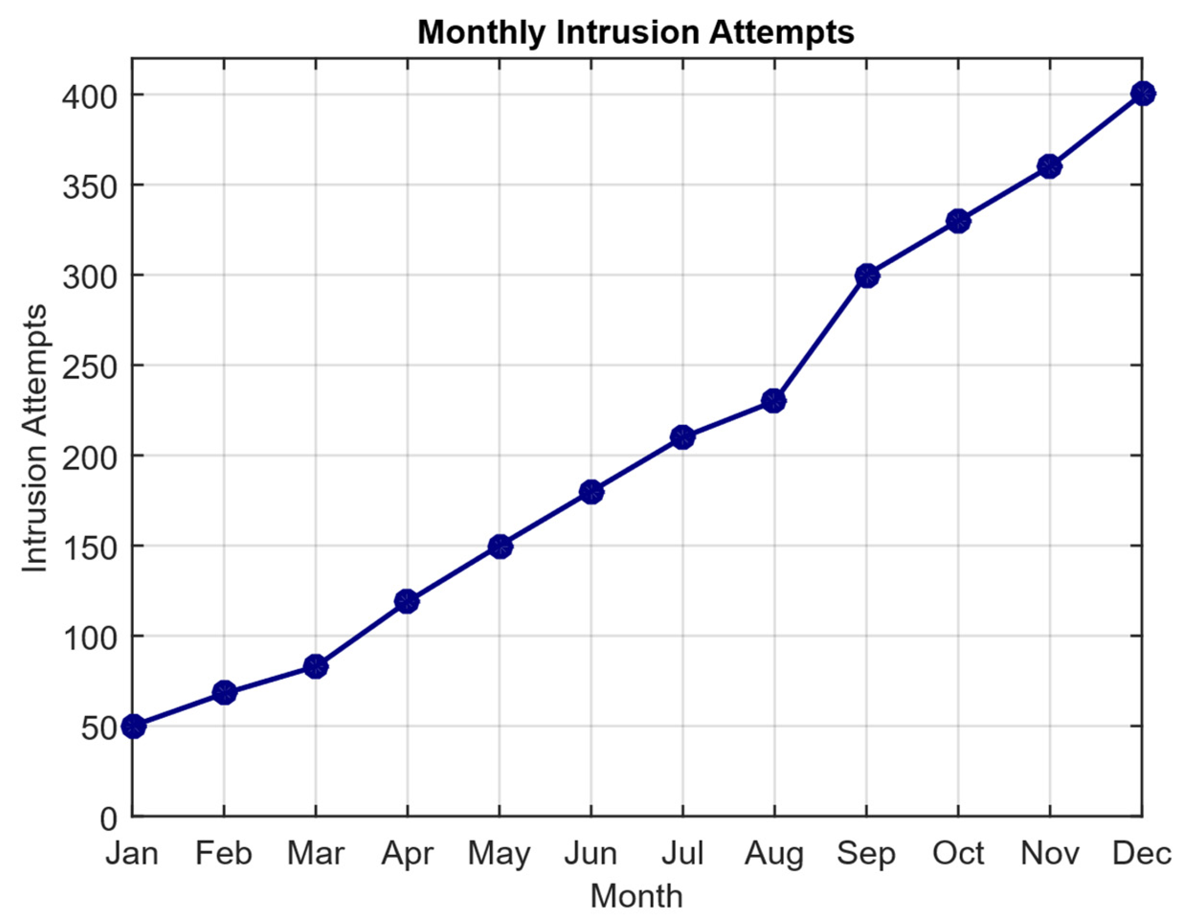
The statistical diagrams (Figure 1 and Figure 2) show two key aspects of threats in the corporate network, namely the attack vectors’ diversity and their occurrence dynamics over time. Figure 1 illustrates that attacks are distributed across different types (scanning, password guessing, malware, DDoS, etc.), with some vectors occurring significantly more frequently. Its changing trend in the intensity of intrusion attempts over time, i.e., an increase in the number, indicates either increased activity by attackers or seasonal spikes in attacks.

Thus, the research relevance is determined by several factors. The increase in the number and complexity of attacks makes traditional signature-based approaches insufficiently effective, as new threats and their variations appear faster than the rules can be updated. At the same time, the growth in the amount of encrypted and polymorphic traffic, as well as the distributed and hidden communication channels used, requires methods capable of detecting anomalies based on behaviour and contextual features, not just static signatures. Corporate networks impose strict requirements on the response speed and the minimization of false positives. In this context, automated prevention and blocking of negatively impacting events should be combined with an allowance level of interference for legitimate users.

In the rapid growth of intelligent technologies, a neural network system with adaptive online training is a promising solution: models that can continuously train from incoming data and adapt to changing traffic patterns can improve detection accuracy and reduce the proportion of false positives. Online training also allows for a quick response to new types of attacks and maintains the detection model’s relevance in a dynamic infrastructure. Thus, such systems implementation helps to improve the corporate network’s information security level by reducing the response time to incidents, reducing the compromise risks, and better complying with access and risk management policies.

2. Related Works

It is known that classical research in the field of IDS/IPS intrusion detection focuses on two main approaches. There are signature (or rule-based) detection and behavioural (anomaly-based) detection. Studies’ results [8,9,10,11] have shown high accuracy (at the 85, …, 90% level) of signature systems in detecting known attacks. At the same time, these results indicate their impotence against new and modified malicious techniques (their detection accuracy does not exceed 17, …, 20%), which brings to the forefront the machine learning methods study for detecting anomalies.

The studies [12,13,14,15] analysis shows the signature [12] and hybrid [13] architectures evolution, demonstrating that the signatures and heuristics combination [14,15] remains a practical basis for commercial products but suffers from scalability issues and support for up-to-date rules in dynamic corporate environments. The key limitation is the high maintenance cost and the need for frequent rule updates, which reduces flexibility when new attack vectors (zero-day and polymorphic variants) appear.

With the advent and development of machine learning and later deep learning methods, machine learning and deep learning approaches to IDS intrusion detection have been actively explored. Tree-based classifiers [16], multilayer perceptron [17], SVM [18], ensembles [19,20,21], LSTM [22,23,24,25], CNN [26,27,28,29], and graph neural networks [30,31] have been applied to recognize complex patterns in network traffic and logs. Deep learning methods [32,33] applications show that deep learning models demonstrate improved ability to extract spatio-temporal features and detect complex attack scenarios, especially in large and feature-rich datasets. However, the key limitations of the machine learning and deep learning approaches include high false positive rates, sensitivity to unbalanced data, significant resource consumption and real-time deployment complexity, and a tendency to degrade in quality when the traffic distribution changes (concept drift). These issues complicate the model’s practical application in online detection tasks in corporate networks.

In response to the changing data distribution and the attacks’ new classes’ continuous emergence problem, research on online training [34], adaptive ensembles [35], drift detection methods [36], and active learning in streaming data [37] has become widespread in recent years. Research [38,39,40,41] proposes mechanisms for concept drift detection (ADWIN [38], DDM [39], etc.), incremental model updating [40], and selective data labelling strategies [41]. However, many of them demonstrate difficulties in obtaining timely and reliable labelling in combat conditions and are computationally intensive.

Recent research in the adaptive architectures field includes hybrid frameworks such as multi-agent [42] and deep novelty-detection approaches [43], active–passive update schemes [44], and the clustering combined use to accumulate evidence of new classes before supervised updating [45]. These studies [42,43,44,45] show that resilience to new and unseen attacks can be improved, but questions remain regarding scalability, update time requirements, and integration with corporate incident response processes.

Research in a separate area in the IDS/IPS intrusion detection field is on methods aimed at reducing false positives. These include adaptive filtering [46], contextual event aggregation [47], and multi-level pipelines [48] (pre-filter, anomaly detector, and signature verifier). Despite the increase in the IDS/IPS intrusion detection accuracy (at the level of 88–91%), the authors of studies [46,47,48] emphasize that the false positive reduction is often achieved at the cost of increasing omissions (false negatives) or increasing response delays, which is unacceptable for some corporate scenarios.

Thus, the above studies demonstrate the transition from static, signature-based systems to hybrid and intelligent (machine learning and deep learning) solutions and, further, to adaptive and online architectures (

Table 1. Review of existing research in the IDS/IPS intrusion detection field.

Study	Approach	Key Contribution	Main Limitations
Systematic machine learning and IDS surveys	Exhaustive review of machine learning methods (supervised or unsupervised)	Algorithms, datasets, metrics systematization	Limitations in practical deployment, real installations lack validation
Deep learning IDS reviews	CNN, RNN, GNN for traffic and logs	Highlighting the deep learning ability to extract complex spatio-temporal features	High computational requirements, sensitive to data imbalances
Adaptive and online IDS (drift detection, ADWIN, DDM)	Streaming algorithms, incremental training	Drift detection and incremental update mechanisms	Markup required, error accumulation risk, and latency when updating
Multi-agent and novelty detection	Deep novelty classifiers with clustering and active labelling	Unseen (zero-day) detection and adaptation	Orchestration complexity, infrastructure requirements, and validation on real networks
Drift-aware ensembles (AdIter or GBDT adaptations)	Ensemble weighting with drift detectors	Fast adaptation of base model weights	Setup complexity, possible increase in computational load

).

However, existing research remains fragmented in a number of respects, including insufficient testing in real corporate networks, weak development of secure model updating issues (how to avoid malicious tweaking), limited support for encrypted traffic, and full integration with SOC/IR operational processes.

Based on the above, the unresolved issues and tasks that directly motivate the neural network system development for detecting and preventing IDS/IPS intrusions with adaptive online training are:

• Ensuring the model’s reliable and safe incremental adaptation in the concept drift conditions without a significant need for manual marking.
• Reducing false positives while maintaining sensitivity to new and hidden attacks.
• Integrating online training into real corporate SOC processes with low latency and an acceptable computing load guarantee.
• Ensuring the model’s stability against targeted tuning (poisoning) and adversarial attacks.
• Attack detection in encrypted and polymorphic traffic, where classic signatures are useless.
• Developing hybrid pipelines of the type “novelty detection → active labelling → incremental supervised update” with accessible risk management and performance metrics.

The described unresolved issues and tasks serve as a technical and scientific justification for the need to develop an adaptive neural network IDS/IPS intrusion detection system capable of quickly training from network data flows and increasing the corporate network’s information security level with minimal human support.

Thus, the research aim is to develop a neural network system for detecting and preventing IDS/IPS intrusions with adaptive online training, capable of increasing detection accuracy in real time, reducing the false positive proportion, and ensuring resistance to traffic distribution drift and targeted attacks in a corporate network. The research object is information and network complexes and processes for ensuring information security of corporate networks, including existing IDS/IPS mechanisms, network traffic, event logs, and SOC (Security Operations Centre) operational procedures. The research subject of study includes methods, architectures, and algorithms for neural network detection and prevention of intrusions with a focus on adaptive (online or incremental) training to extract features from network traffic and logs, mechanisms for detecting concept drift and novel attacks, strategies for safely updating models, and their integration into incident prevention workflows.

The research makes a significant contribution to the IDS/IPS intrusion detection and prevention field by developing an original neural network architecture for IDS/IPS intrusion detection and prevention with adaptive online training, including a secure incremental model update algorithm, concept-drift detection and poisoning protection mechanisms, as well as a multi-level false alarm reduction strategy and a methodology for integration into SOC processes, which ensures high detection accuracy (more than 92, …, 94%), resistance to traffic changes, and practical applicability in corporate networks.

This article consists of traditional sections: “1. Introduction”, “2. Related Works”, “3. Materials and Methods”, “4. Case Study”, “5. Discussion”, and “6. Conclusions”. In Section 3, we formalize the theoretical foundations for intrusion detection and prevention (using LRT, GLR, SPRT, CUSUM, and information measures such as the Kullback–Leibler divergence and the Chernoff coefficient), substantiate the context-adaptive threshold advantages, and prove the minimax properties in a number of settings. In parallel, we introduce a model of robustness to targeted adjustments and poisoning (Huber-ε, clipped, and inf-LR criteria) with FPR/TPR shift estimates and “headroom” conditions to preserve sensitivity. We propose a complex hybrid architecture consisting of modal encoders for traffic and logs, a temporal GNN for entity correlation, a KV memory, a variational module for uncertainty, a differentiable symbolic unit, an RL agent for prioritization, and an NLG module for explanations, all united by a common multi-task learning. A computational cost analysis is performed (approximately 2.17 · 10⁹ FLOPs of forward-run), with practical recommendations for optimization (local and linear approximation of attention, mixed-precision, caching, and sampling in GNN) and pointing out key limitations, which include sensitivity to the correctness of context modelling, the need for high-quality labelled multi-modal data, high computational cost, and the need for verification and hyperparameter selection during deployment. Section 4 describes the preparation and preprocessing of a multimodal experimental dataset (synchronized traffic time series, logs, and telemetry with simulated DDoS), a multi-stage protocol for hybrid model training and online adaptation, a virtual instance implementation with an incident interface and NLG explanations, detailed quantitative results (AUC ≈ 0.95, F1 ≈ 0.95), and a drift resilience with metric recovery study through accurate incremental adaptation. Practical recommendations for optimizations, computational cost estimation, and legal and forensic readiness requirements are also offered. Limitations, including the need for high-quality labelled data, significant deployment resources, and the need for standardized benchmarks for reproducibility, are highlighted. In the Discussion section, the authors summarize their contributions (formal justifications for context-adaptive thresholds and minimax-robust rules, hybrid multimodal architecture, and online training), while also noting limiting factors such as the need for high-quality labelled and contextual data, computational infrastructure, rigorous benchmark validation, and legal training for using the artifacts in law enforcement practice.

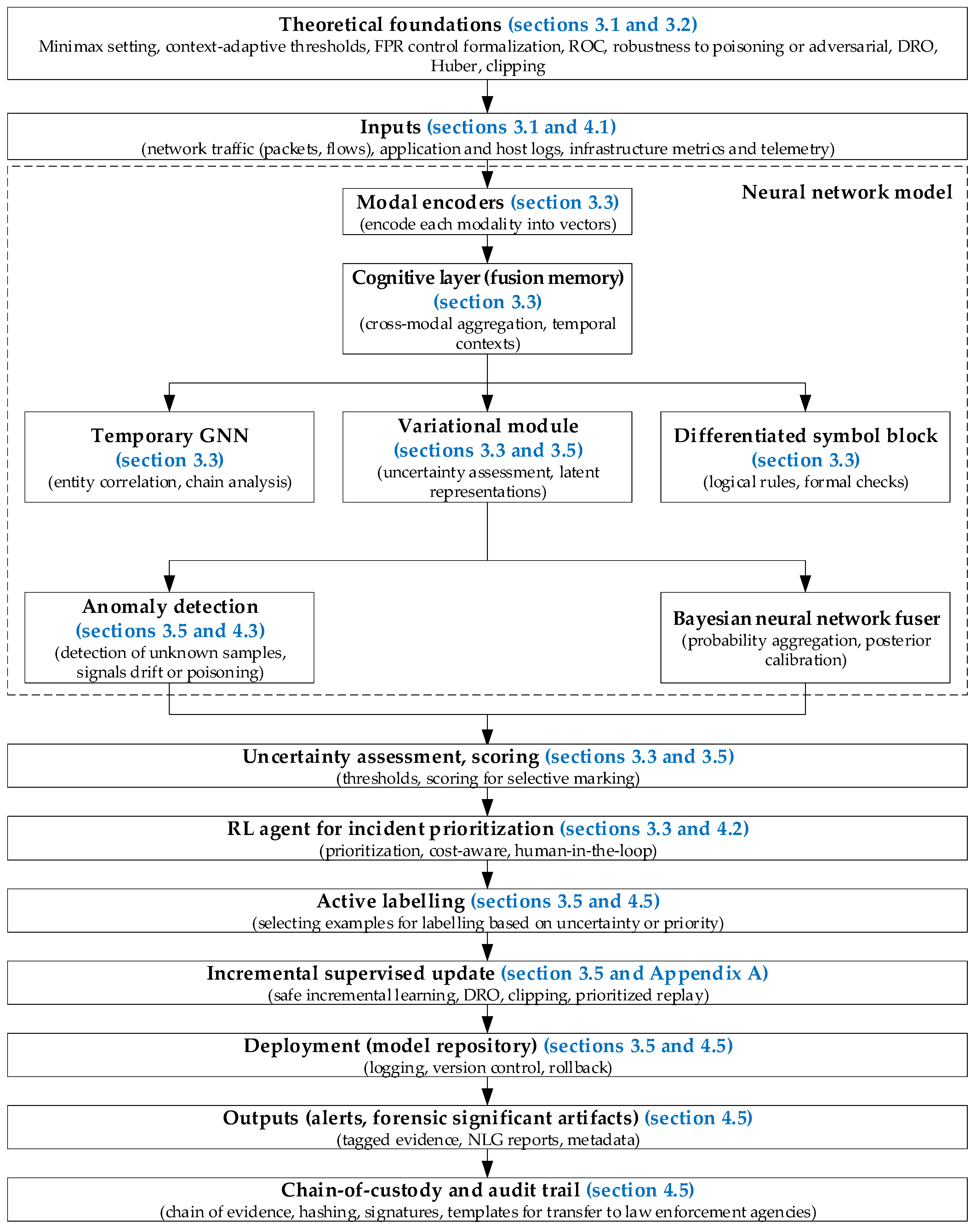
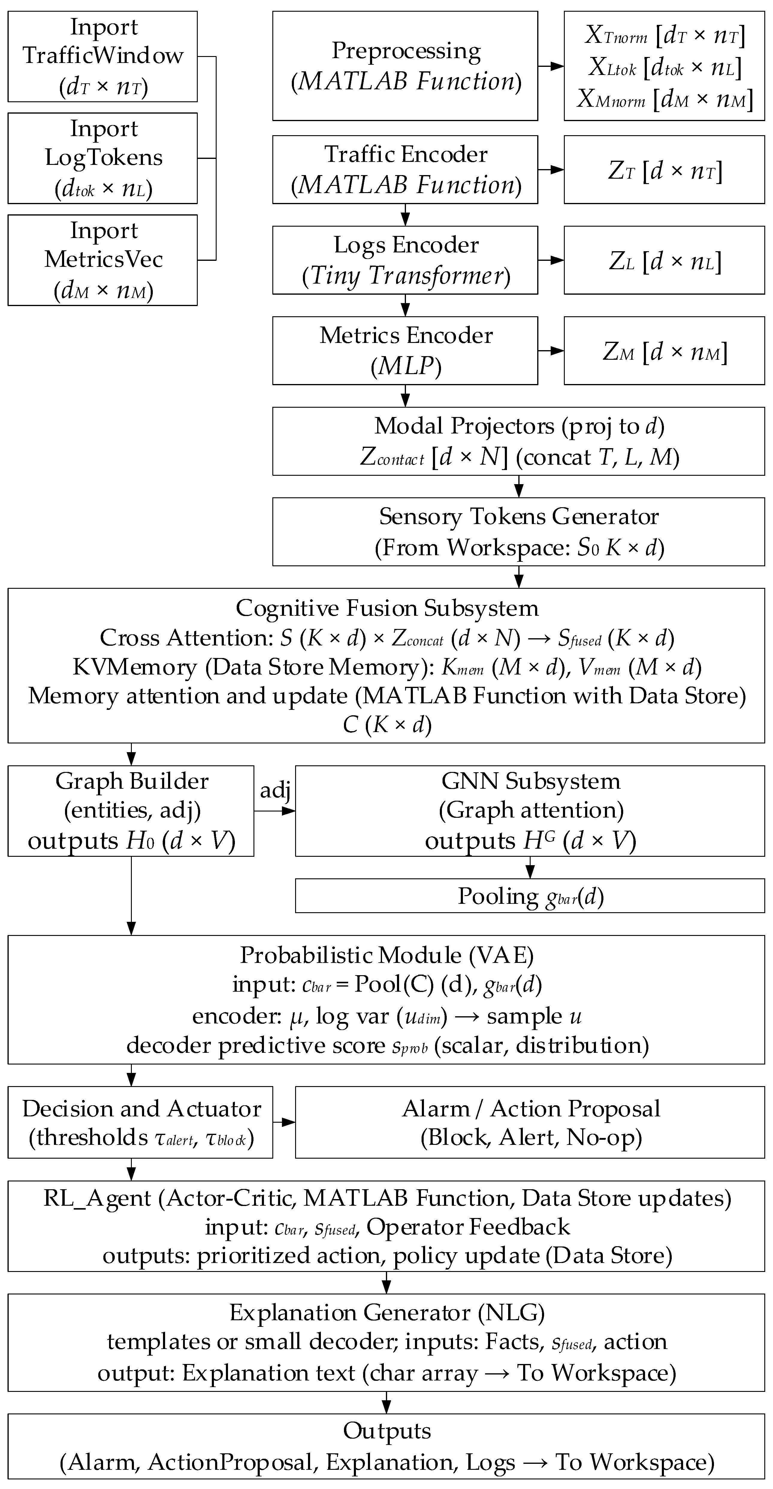
Based on the above, this study proposes a solution (Figure 3) based on a hybrid multimodal architecture. Network flows, logs, and telemetry are encoded by modal encoders and combined in a cross-modal fusion memory to construct a unified incident context. A temporal GNN ensures entity correlation and the complex relations identification, a variational module formalizes uncertainty, and a differentiable symbolic block embeds formal rules and improves explainability. A Bayesian neural network fuser aggregates probabilistic estimates and transmits novelty or anomaly detection signals to the uncertainty scoring subsystem. An RL agent and prioritization mechanisms guide the selective labelling process by experts (active labelling), whose results are used for secure incremental model updates while preserving audit trails. The custody protocols and NLG module chain produce verifiable artifacts and calibrated alerts, guaranteeing drift resistance and forensic suitability.

3. Materials and Methods

3.1. Development of Theoretical Foundations for the IDS/IPS Intrusion Detection and Prevention

Consider an observation flow (network telemetry) in discrete time t = 1, 2, … Each observation is a feature vector X_t ∈ ℝ^d. In the idealized model, there is a “normal” (without attack) probability distribution P₀ with density p₀(x) and a “malicious” distribution P₁ (or one P₁) family with density p₁(x). The detector task is to establish the difference between hypotheses based on the observed data {X_t}:

H₀: X_t ∼ P₀ (no attack) and H₁: X_t ∼ P₁ (there is an attack).

(1)

The classical approach [8,10,11] compares the likelihood and constructs tests based on the likelihood ratio. Let us introduce the likelihood ratio function of the form:

$$\mathsf{\Lambda }\left(x\right):={\displaystyle \frac{p_1\left(x\right)}{p_0\left(x\right)}}.$$

(2)

For observations set x = (x₁, …, x_n), the likelihood ratio is

$${\mathsf{\Lambda }}_n\left(\mathbf{x}\right)={\displaystyle \prod _{t=1}^n}{\displaystyle \frac{p_1\left(x\right)}{p_0\left(x\right)}}=\left(\exp \sum _{t=1}^n\log \left({\displaystyle \frac{p_1\left(x_t\right)}{p_0\left(x_t\right)}}\right)\right).$$

(3)

For simple hypotheses (when P₀ and P₁ are completely specified), the Neyman–Pearson criterion [49,50] gives the optimal rule: reject H₀ if Λ_n(x) > η, or

$${\displaystyle \sum _{t=1}^n}\log \left({\displaystyle \frac{p_1}{p_0}}\right)>\log \eta ,$$

(4)

which provides maximum power at a fixed significance level α.

If P₀ and P₁ are multivariate normal $\mathcal{N}$(μ₀, Σ) and $\mathcal{N}$(μ₁, Σ) (that is, their covariances are equal), then the log-likelihood ratio for a single observation is:

$$\log \mathsf{\Lambda }\left(x\right)=-{\displaystyle \frac{1}{2}}·{\left(x-{\mu }_1\right)}^{\top }·{\mathsf{\Sigma }}^{-1}·\left(x-{\mu }_1\right)+{\displaystyle \frac{1}{2}}·{\left(x-{\mu }_0\right)}^{\top }·{\mathsf{\Sigma }}^{-1}·\left(x-{\mu }_0\right),$$

(5)

which reduces to a linear function of the form:

$$\log \mathsf{\Lambda }\left(x\right)=-{\displaystyle \frac{1}{2}}·{\left({\mu }_1-{\mu }_0\right)}^{\top }·{\mathsf{\Sigma }}^{-1}·x-{\displaystyle \frac{1}{2}}·\left({\mu }_1^{\top }·{\mathsf{\Sigma }}^{-1}·{\mu }_1-{\mu }_0^{\top }·{\mathsf{\Sigma }}^{-1}·{\mu }_0\right),$$

(6)

Thus, the optimal test is reduced to the linear discriminant (Fisher LDA) [51]. If the covariances differ, the test becomes quadratic. To assess deviations from normal behaviour, the Mahalanobis distance is used [52,53]:

$$D^2\left(x\right)={\left(x-{\mu }_1\right)}^{\top }·{\mathsf{\Sigma }}^{-1}·\left(x-{\mu }_0\right),$$

(7)

and with real normality $D^2~{\chi }_d^2$, hence the threshold by quantile ${\chi }_d^2\left(1-\alpha \right)$ gives the criterion of an outlier (anomaly).

When the parameters μ and Σ are unknown, the generalized likelihood ratio (GLR) of the form [54] is applied:

$${\mathsf{\Lambda }}_n^{GLR}={\displaystyle \frac{{\sup }_{\theta \in {\mathsf{\Theta }}_1}L\left(\theta ;\mathbf{x}\right)}{{\sup }_{\theta \in {\mathsf{\Theta }}_0}L\left(\theta ;\mathbf{x}\right)}}, L\left(\theta ;\mathbf{x}\right)=\prod _{t=1}^n{p}_0\left(x_t\right).$$

(8)

According to Wilks’ theorem, under correct regular conditions (and when H₀ is true), the statistic

$$-2·{\mathsf{\Lambda }}_n^{GLR}\stackrel{d}{\Rightarrow }{\chi }_k^2,$$

(9)

where k = dim(Θ) − dim(Θ₀), which gives asymptotic criteria for testing complex hypotheses and thresholds, which is a typical approach for “change detection” when the model is parameterized but the parameters are not known in advance.

Sequential tests are essential for online (or sequential) attack detection. Let successive observations be independent (or conditionally independent), and let us want to detect the transition from P₀ to P₁ as quickly as possible while maintaining the average false positive rate. The classic SPRT (Sequential Probability Ratio Test, Wald) uses the cumulative log-ratio of the form [55]:

$$S_n=\sum _{t=1}^n\log \left({\displaystyle \frac{p_1\left(X_t\right)}{p_0\left(X_t\right)}}\right).$$

(10)

The basic rule is to stop and accept H₁ if S_n ≥ log(B) or stop and accept H₀ if S_n ≤ log(A), otherwise continue calculating the cumulative log ratio (11). The threshold values A and B are chosen through the desired error levels α and β, approximately as

$$A={\displaystyle \frac{\beta }{1-\alpha }}, B={\displaystyle \frac{\alpha }{1-\beta }},$$

(11)

that is, asymptotically. SPRT minimizes the average number of observations among all tests with given errors (Wald optimality). CUSUM [56] is a modification for detecting shifts in flows. We define

$$\begin{gathered} g\left(X_t\right)=\log \left({\displaystyle \frac{p_1\left(X_t\right)}{p_0\left(X_t\right)}}\right), \\ {W}_n=\max \left\{0,W_{n-1}+g\left(X_n\right)\right\}, \\ {W}_0=0, \end{gathered}$$

(12)

and signal if W_n ≥ h, with the threshold h selected to match the average run length (ARL) limit. CUSUM is effective for quickly detecting small, constant shifts. The error criteria are the false positive rate and the detection probability (true positive rate, sensitivity), defined as:

$$\begin{gathered} FPR=\mathrm{P}\mathrm{r}\left(\mathrm{a}\mathrm{l}\mathrm{a}\mathrm{r}\mathrm{m}|H_0\right), \\ TPR=\mathrm{P}\mathrm{r}\left(\mathrm{a}\mathrm{l}\mathrm{a}\mathrm{r}\mathrm{m}|H_1\right). \end{gathered}$$

(13)

The ROC curve is constructed parametrically by the threshold τ from the dependence (FPR(τ), TPR(τ)). For LRT, the theoretical expression for TPR and FPR is:

$$\begin{gathered} FPR\left(\eta \right)=\underset{x:\mathsf{\Lambda }\left(x\right)>\eta }{\int }{p}_0\left(x\right)dx, \\ TPR\left(\eta \right)=\underset{x:\mathsf{\Lambda }\left(x\right)>\eta }{\int }{p}_1\left(x\right)dx. \end{gathered}$$

(14)

The information metric underlying the detection rate is the Kullback–Leibler divergence (KL divergence) [57]:

$$D_{KL}\left(P_1‖P_0\right)={\mathbb{E}}_{P_1}\left[\log \left({\displaystyle \frac{p_1\left(X_t\right)}{p_0\left(X_t\right)}}\right)\right].$$

(15)

For a sequential detector with a low false alarm rate, the average detection time $\mathbb{E}$[τ] is inversely proportional to the Kullback–Leibler divergence, that is:

$$\mathbb{E}\left(\tau \right)\approx {\displaystyle \frac{\left|\log \left(\alpha \right)\right|}{D_{KL}\left(P_1‖P_0\right)}}.$$

(16)

For anomalies that cannot be described well parametrically, reconstruction methods [58,59] or autoencoders [60,61] are used. Let the data be centred and the data matrix X ∈ ℝ^n×d have SVD X = U · Σ · V^⊤. Then the projection onto the first k components yields the reconstruction:

$$\widehat{x}=V·V_k^{\mathrm{\top }}·x,$$

(17)

And in this case, the reconstruction error is defined as:

$$\epsilon \left(x\right)={‖x-\widehat{x}‖}^2=\sum _{j=k+1}^d{\left(v_j^{\mathrm{\top }}·x\right)}^2.$$

(18)

An anomaly is detected if ε(x) > τ. PCA gives an optimal linear reconstruction of rank k in the lower mean square error terms. In the stochastic approach, ε(x) can be normalized, and thresholds based on the error distribution can be used. It is known that machine learning methods are used as classifiers. For example, logistic regression builds a model:

$$\mathrm{P}\mathrm{r}\left(\mathrm{Y}=1|x\right)=\sigma \left({\omega }^{\mathrm{\top }}·x+b\right), \sigma \left(z\right)={\displaystyle \frac{1}{1+e^{-z}}}.$$

(19)

The parameters ω and b estimates are obtained by maximum likelihood (the logistic loss minimization). It is known that the support vector machine (SVM) solves the problem:

$$\underset{\omega ,b}{\min }\left({\displaystyle \frac{1}{2}}·{‖\omega ‖}^2+C·\sum _i{\xi }_i\right), \mathrm{s}.\mathrm{t}.y_i·\left({\omega }^{\mathrm{\top }}·x_i+b\right)\ge 1-{\xi }_i, {\xi }_i\ge 0,$$

(20)

and gives a linear or kernel boundary between “norm” and “attack”. ROC (AUC), precision, F1-score, and standard metrics are used for quality assessment. Classifiers require the selection of X_t features, such as duration, bytes, packets, entropy indicators, etc., and data balancing (in reality, attacks are rare).

For the false positives statistical guarantee, concentration inequalities (Chernoff, Hoeffding [62,63]) are used, that is, if g(X) has bounded moments, then for n observations,

$$\mathrm{Pr}\left({\displaystyle \frac{1}{n}}·\sum _{t=1}^{n}g\left(X_t\right)-\mathbb{E}\left[g\left(X\right)\right]\ge ϵ\right)\le \exp -n·I\left(ϵ\right),$$

(21)

where I(ϵ) depends on a moment-generating function, which gives exponential estimates of the erroneous threshold exceedance probability and allows thresholds to be linked to the desired false alarm rate.

In prevention problems, the models are extended [17,20,23,27], and the detector can apply blocking or slowdowns (rate-limiting) according to the rule π. Let the action π lead to losses L(π, θ) under the attacker’s strategy θ. Then the defender’s task is to minimize the expected losses under unknown θ. It is naturally formalized as a private information game or a Stackelberg game, that is, the defender chooses a policy (leader), and the attacker reacts optimally. In the simplest case, let us assume that a threshold τ specifies the detector, and the attacker chooses an attack intensity λ. Then the attacker’s utility is represented as:

U_A(λ, τ) = g(λ) − c · Pr(detection(λ, τ)),

(22)

and the defender utility as:

U_D(τ, λ) = −L(λ) · Pr(detection) − C_false · Pr(FP),

(23)

The search for equilibrium yields first-order conditions of the form:

$${\displaystyle \frac{\partial U_A}{\partial \lambda }}=0, {\displaystyle \frac{\partial U_D}{\partial \tau }}=0,$$

(24)

which leads to a system of equations for (τ*, λ*). It is important to note that when modelling, the defender must take into account incomplete information and uncertainty in the attack parameters—the Bayesian approach with a prior on θ is correct.

To reduce false positives while maintaining sensitivity to new and hidden attacks, it is assumed that X ∈ $\mathcal{X}$ is an observation (packet feature vector, flow, or aggregation), and Z ∈ $\mathcal{Z}$ is a context. Under the null hypothesis (no attack), the pair (X, Z) distribution is given by the measure P₀ with density (by the corresponding measures) p₀(x, z).

The possible attack set is modelled as an alternative distribution family {P_θ: θ ∈ Θ} with densities p_θ(x, z). The detector operates according to an arbitrary measurable rule δ: $\mathcal{X}$ × $\mathcal{Z}$ → {0, 1} (1 is the “attack” signal). The FPR is assumed to be defined as:

$$FPR\left(\delta \right)=R_0\left(\delta \right)≔{\mathbb{E}}_{P_0}\left[\delta \left(X,Z\right)\right]=\int \delta \left(x,z\right)·p_0\left(x,z\right)dxdz,$$

(25)

and for the attack parameter, θ is the sensitivity (TPR), defined as:

$$TPR\left(\delta \right)=R_{\theta }\left(\delta \right)≔{\mathbb{E}}_{P_{\theta }}\left[\delta \left(X,Z\right)\right]=\int \delta \left(x,z\right)·p_{\theta }\left(x,z\right)dxdz.$$

(26)

The key task is to reduce R₀(δ) while requiring that the detector remain sensitive to any “strong enough” attacks from some set Θ. We formalize this as an optimization problem with a hard constraint on the worst-case TPR:

$$\begin{gathered} \mathrm{minimize} R_0\left(\delta \right) \mathrm{given\; that} \\ \underset{\theta \in \mathsf{\Theta }}{\inf } R_{\theta }\left(\delta \right)\ge \gamma , \end{gathered}$$

(27)

where γ ∈ (0, 1) is a given target sensitivity level (e.g., γ = 0.95). This formulation reflects the requirement to “maintain sensitivity to new and hidden attacks” in the worst-case sense. To do this, it is necessary to study the structure of the optimal solution, show how the contextual information Z is used and the “best” mixed alternative (least-favourable prior) choice reduces R₀, and formulate and prove the theorem on the context-adaptive thresholding strict gain. It is assumed that the conditional probability densities are given as:

$$p_0\left(x|z\right)={\displaystyle \frac{p_0\left(x,z\right)}{q_0\left(z\right)}}, p_{\theta }\left(x|z\right)={\displaystyle \frac{p_{\theta }\left(x,z\right)}{q_{\theta }\left(z\right)}},$$

(28)

where $q_0\left(z\right)=\int p_0\left(x,z\right)dx$ and $q_{\theta }\left(z\right)=\int p_{\theta }\left(x,z\right)dx$ are the marginals with respect to Z. A critical typical case is that the Z context does not depend on the attack (e.g., daytime, routing scheme, relative network load), and the marginal q(z) is common to P₀ and P_θ. Let us consider the general case and then a separate special case, q_θ(z) = q(z) ∀ θ.

The general case key idea is to construct a context-conditional likelihood ratio (LR) or its approximation instead of a single “voting” score and to threshold the conditional LR. It is the conditional LR thresholding that is optimal (in the FPR minimizing sense under the constraint on the conditional or nested TPR), which is expressed through the Neyman–Pearson lemma conditional version [64]. To do this, we define for an arbitrary mixture (prior) π on Θ its mixed density as:

$$p_{\pi }\left(x|z\right):=\underset{\mathsf{\Theta }}{\int }{p}_{\theta }\left(x,z\right)\pi \left(d\theta \right).$$

(29)

Its conditional LR with respect to P₀ is defined as:

$$L_{\pi }\left(x|z\right):={\displaystyle \frac{p_{\pi }\left(x|z\right)}{p_0\left(x|z\right)}}={\displaystyle \frac{\int \frac{p_{\theta }\left(x,z\right)\pi \left(d\theta \right)}{q_{\pi }\left(z\right)}}{\frac{p_0\left(x,z\right)}{q_0\left(z\right)}}}={\displaystyle \frac{\int p_{\theta }\left(x,z\right)\pi \left(d\theta \right)}{p_0\left(x,z\right)}}·{\displaystyle \frac{q_0\left(z\right)}{q_{\pi }\left(z\right)}}.$$

(30)

If the marginal q_θ(z) ≡ q₀(z) (special case), then

$$L_{\pi }\left(x|z\right)={\displaystyle \frac{\int p_{\theta }\left(x,z\right)\pi \left(d\theta \right)}{p_0\left(x,z\right)}}.$$

(31)

Consider the test. δ_π,τ(x, z) = 1{L_π(x ∣ z) ≥ τ(z)} is the conditional mixed density thresholding mixture at a threshold possibly depending on z. Of particular interest are two classes of thresholds. There are an inflexible (global) threshold τ(z) ≡ τ (does not take into account the context) and a context-adaptive threshold τ(z), which can vary with z. Thus, it is necessary to show that, given the prior π* optimal choice (least-favourable prior) and the optimal context threshold τ*(z), the algorithm δ_π*,τ* minimizes FPR at the sensitivity required in the inf_θ-level, and it gives no worse, and often strictly better, R₀ than the optimal constant threshold.

Theorem 1. 

Context-adaptive false alarm minimization.

Let {P_θ: θ ∈ Θ} be an alternative distribution family, and let P₀ be an attack-free distribution. Assume that all measures are absolutely filling (have densities) and the solution space is measurable. For a given γ ∈ (0, 1), there exists a least-favourable prior π* on Θ and a threshold context function τ*(z) such that the test:

$${\delta }^{*}\left(x,z\right)=\mathbf{1}\left\{L_{{\pi }^{*}}\left(x|z\right)\ge {\tau }^{*}\left(z\right)\right\}$$

(32)

solves the minimizing R₀(δ) problem among all measurable rules δ with $\underset{\theta \in \mathsf{\Theta }}{\inf } R_{\theta }\left(\delta \right)\ge \gamma$. Moreover, if there exists z with non-trivial context dependence of LR (i.e., the density ratio ${\displaystyle \frac{p_{\theta }\left(•|z\right)}{p_0\left(•|z\right)}}$ distribution depends on z for at least two θ), then the context-adaptive threshold τ*(z) yields strictly lower false alarms than any optimal global (z-independent) test, all else being equal (i.e., purely adaptive if LR is context-dependent).

Proof of Theorem 1. 

To prove the problem equivalence and the minimax problem, we consider the maximizing dual problem, the worst-case TPR with a fixed false alarm rate α:

$$\mathsf{\Phi }\left(\alpha \right)=\underset{\delta :R_0\left(\delta \right)\le \alpha }{\sup }\underset{\theta \in \mathsf{\Theta }}{\inf } R_{\theta }\left(\delta \right).$$

(33)

The function Φ(α) is non-increasing in α. Then the original problem is to find $\underset{\theta }{\min } R_0\left(\delta \right)$ for $\underset{\theta }{\inf } R_{\theta }\left(\delta \right)\ge \gamma$, which is equivalent to finding α* = inf(α: Φ(α) ≥ γ). The compactness standard argument, i.e., weak upper semi-convexity (in probability measure spaces) and the minimax principle (Sion or von Neumann), ensures the existence of an optimal pairwise strategy, i.e., there is a prior π* such that

$$\mathsf{\Phi }\left(\alpha \right)=\underset{\delta :R_0\left(\delta \right)\le \alpha }{\mathrm{s}\mathrm{u}\mathrm{p}}\int R_{\theta }\left(\delta \right){\pi }^{*}\left(d\theta \right)=\underset{\delta :R_0\left(\delta \right)\le \alpha }{\mathrm{s}\mathrm{u}\mathrm{p}}{R}_{{\pi }^{*}}\left(\delta \right),$$

(34)

where $R_{\pi }\left(\delta \right)=\int R_{\theta }\left(\delta \right)\pi \left(d\theta \right)={\mathbb{E}}_{P_{\pi }}\left[\delta \right]$, that is, the worst-case alternative is “replaced” by some mixture $P_{{\pi }^{*}}$, which is the least-favourable prior (That is, the convex-compact properties of all the rules in the δ set in the weak topology and the linear functionals R₀ convexity and R_θ are formally applied).

For a fixed π*, the problem $\underset{\delta :R_0\left(\delta \right)\le \alpha }{\mathrm{s}\mathrm{u}\mathrm{p}}{R}_{{\pi }^{*}}\left(\delta \right)$ is the detecting the H₀ problem: P₀ against H₁: $P_{{\pi }^{*}}$. By the Neyman–Pearson lemma, the optimal rule in this problem (for a given α) is the test that thresholds the likelihood ratio between $P_{{\pi }^{*}}$ and P₀. Thus, the optimal test is:

$${\delta }^{NP}\left(x,z\right)=\mathbf{1}\left\{{\displaystyle \frac{p_{{\pi }^{*}}\left(x,z\right)}{p_0\left(x,z\right)}}\ge \eta \right\}$$

(35)

with the corresponding randomness occurs at the boundary, such that ${\mathbb{E}}_{P_0}\left[{\delta }^{NP}\right]=\alpha$. Then (35) can be rewritten as:

$${\delta }^{NP}\left(x,z\right)=\mathbf{1}\left\{L_{{\pi }^{*}}\left(x|z\right)\ge \tau \left(z\right)\right\},$$

(36)

where τ(z) is obtained from η and normalizations with respect to z. Thus, the optimal rule against a mixture with respect to π* is the conditional LR thresholding. Combining the above, we obtain:

$${\alpha }^{*}=\min R_{\theta }\left(\delta \right)$$

(37)

for $\underset{\theta }{\inf } R_{\theta }\left(\delta \right)\ge \gamma$. This indicates a prior π* existence and a corresponding threshold τ*(z) at which ${\delta }^{*}\left(x,z\right)=\mathbf{1}\left\{L_{{\pi }^{*}}\left(x|z\right)\ge {\tau }^{*}\left(z\right)\right\}$ reaches the optimum.

To strictly improve the context-adaptive threshold over the optimal global threshold, it is assumed that for all z, the LR conditional law of x, that is, the function distribution:

$${\mathcal{\ell }}_{\theta }\left(x|z\right):={\displaystyle \frac{p_{\theta }\left(x|z\right)}{p_0\left(x|z\right)}},$$

(38)

is not identical in z, that is, there exist z₁, z₂, θ₁, and θ₂ such that the ${\mathcal{\ell }}_{{\theta }_{\mathbf{1}}}\left(•|z_{\mathbf{1}}\right)$ and ${\mathcal{\ell }}_{{\theta }_2}\left(•|z_2\right)$ distributions are different. For the sake of contradiction, it is assumed that some optimal global test ${\delta }_{glob}\left(x,z\right)=\mathbf{1}\left\{L_{{\pi }^{*}}\left(x|z\right)\ge \overline{\tau }\right\}$ (the threshold $\overline{\tau }$ does not depend on z) yields the same FPR level as the context-adaptive δ*. Then by construction, both strategies are equivalent almost everywhere with respect to P₀: the threshold sets differ in P₀-measure zero. But since the conditional LR distributions differ in z, one can select a threshold shift τ(z) (lower τ for “similar” contexts and increase it for “noisy” ones) to preserve $\underset{\theta }{\inf } R_{\theta }$ and simultaneously reduce ${\mathbb{E}}_{P_0}\left[\delta \right]$ to recalculate the signal regions measured under P₀. It is achievable because changing τ(z) on sets with high q₀(z) and a favourable density ratio will give a negative derivative w.r.t. R₀ while preserving $R_{{\pi }^{*}}$. Formally, considering the variation τ(z) ↦ τ(z) + ϵ(z) and a linear increment in the first orders, we obtain the decreasing R₀ direction, remaining in the admissible set due to tuning on different z. Therefore, if the conditional LR really depends on the context, there is a decrease in R₀, i.e., the context-adaptive threshold is strictly better. If LR does not depend on z (the conditional LR is the same everywhere), then adaptivity does not give anything. The theorem is proved. □

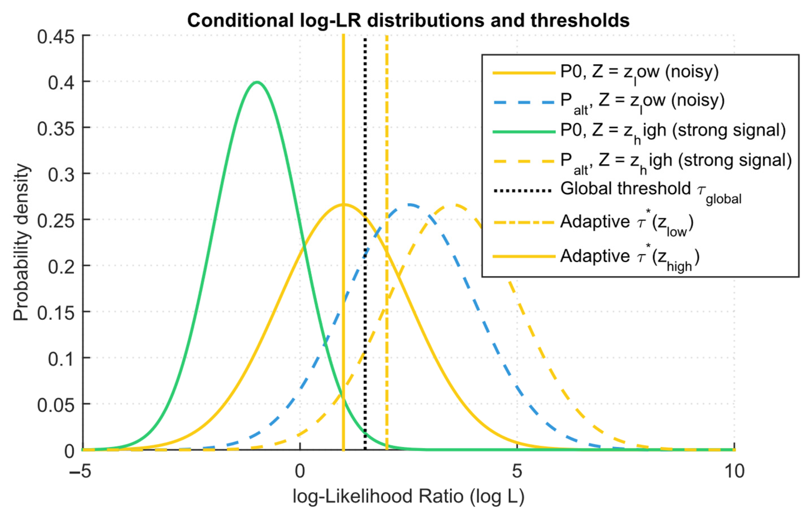
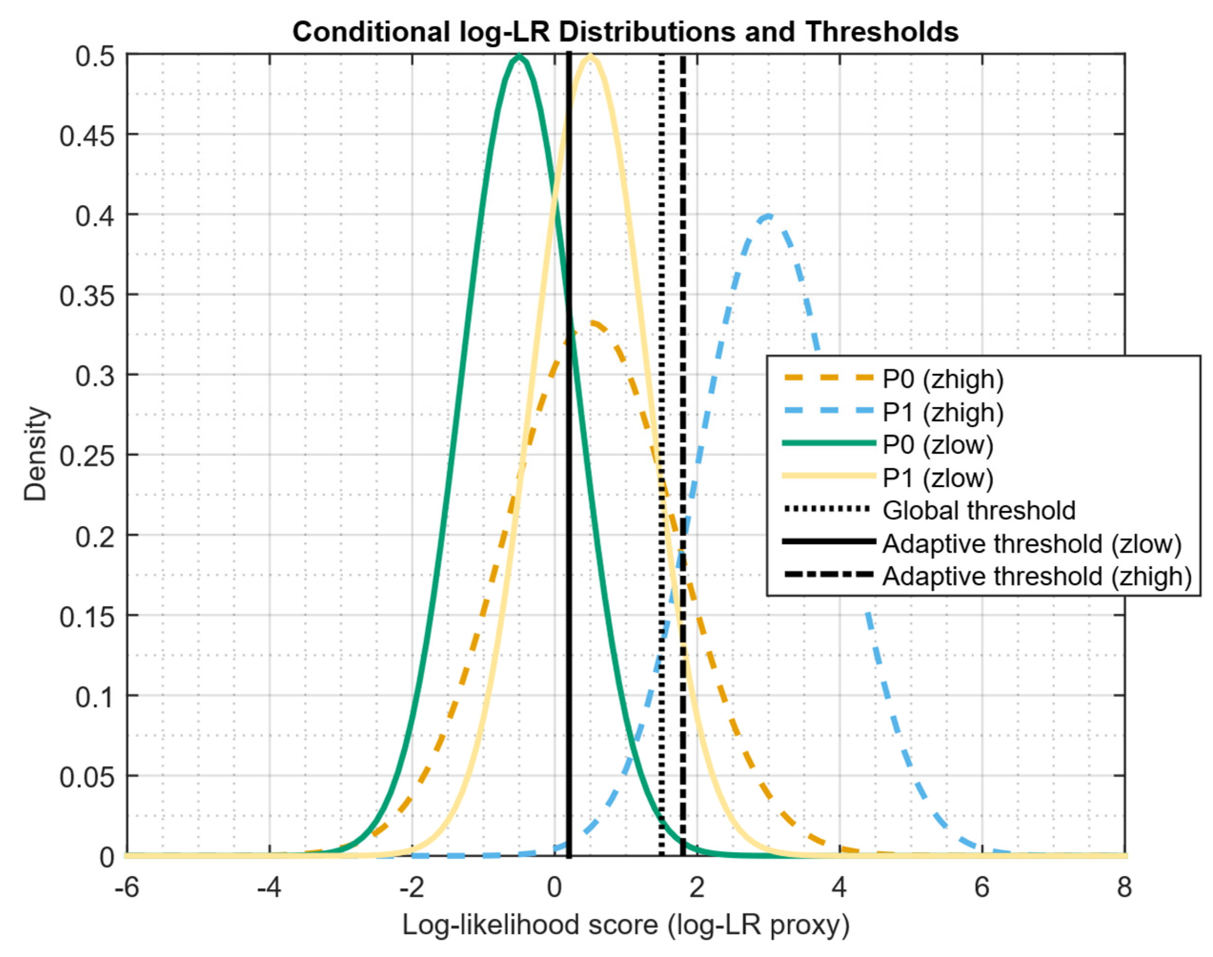
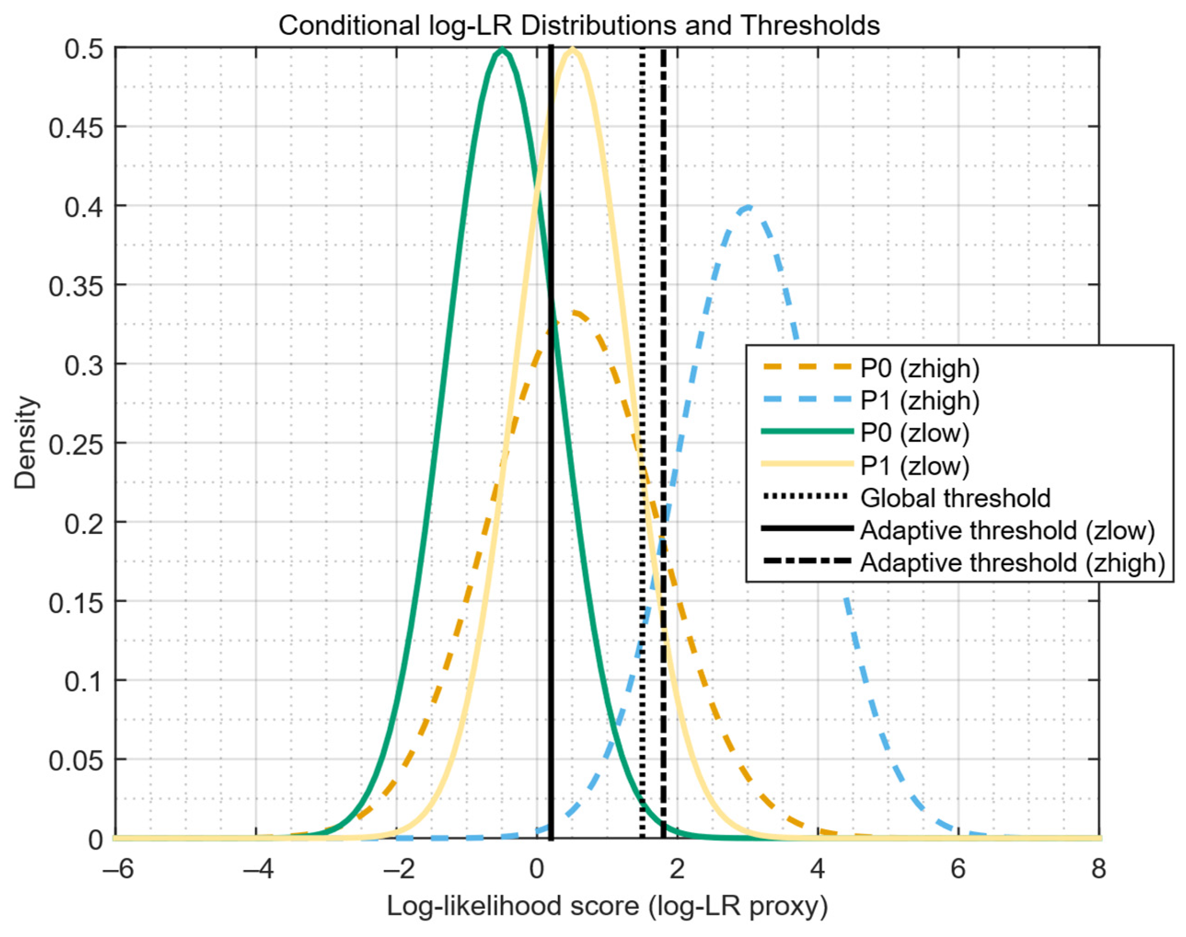
Figure 4 illustrates Theorem 1’s key idea, since a z-dependent threshold allows us to reduce the FPR for a fixed worst-case sensitivity by shifting the threshold in “good” contexts (z_high in Figure 4) towards smaller values, where the alternative distribution is further removed from the null hypothesis. In “noisy” contexts (z_low in Figure 4), the adaptive threshold rises, reducing the contribution to the overall FPR. Figure 4 shows that for the same overall TPR, the error areas in P₀ are smaller in the adaptive thresholds case compared to using a single global threshold.

Thus, a Theorem 1 corollary is if the context Z is informative (the conditional LR varies with z), then in the FP reduction problem with a fixed worst-case sensitivity, the contextual adaptation gain is positive. Equivalently, the threshold depending on z is always no worse than the global threshold and strictly better when the conditional LRs are not constant.

To obtain analytical expressions for numerical optimization and to estimate the size of the FP reduction, it is assumed that for fixed π* and fixed z, we consider the conditional LR distributions under P₀ and under $P_{{\pi }^{*}}$. Since it is not always possible to express τ*(z) analytically in a closed manner, we can set the condition for τ*(z) as a solution to the equation:

$${\mathbb{E}}_{{\pi }^{*}}\left[\left.\mathbf{1}\left\{L_{{\pi }^{*}}\left(X|z\right)\ge {\tau }^{*}\left(z\right)\right\}\right|Z=z\right]=\beta \left(z\right),$$

(39)

and require $\int \beta \left(z\right)q_{\pi }\left(z\right)dz=\gamma$ (summed over z, the worst-case TPR reaches γ). In practice, β(z) is chosen to minimize ${\mathbb{E}}_{P_0}\left[\left.\mathbf{1}\left\{L_{{\pi }^{*}}\left(X|z\right)\ge {\tau }^{*}\left(z\right)\right\}\right|Z=z\right]$ for a given total sensitivity.

For specific models (e.g., conditionally standard), more explicit expressions are obtained. Let us assume that for a fixed z,

$$X⌈Z=z~\left\{\begin{array}{c}\mathcal{N}\left({\mu }_0\left(z\right), \mathsf{\Sigma }\left(z\right)\right), H_0\\ \mathcal{N}\left({\mu }_{\theta }\left(z\right), \mathsf{\Sigma }\left(z\right)\right), H_{\theta }\end{array}\right.$$

(40)

and let the marginal q(z) be the same for all. Then the conditional LR (using a mixed alternative) has the form:

$$\log L_{\pi }\left(x|z\right)={\left(\overline{\mu }\left(z\right)-{\mu }_0\left(z\right)\right)}^{\mathrm{\top }}·\mathsf{\Sigma }{\left(z\right)}^{-1}·x-{\displaystyle \frac{1}{2}}·\left(\overline{\mu }{\left(z\right)}^{\mathrm{\top }}·\mathsf{\Sigma }{\left(z\right)}^{-1}·\overline{\mu }\left(z\right)-{\mu }_0{\left(z\right)}^{\mathrm{\top }}·\mathsf{\Sigma }{\left(z\right)}^{-1}·{\mu }_0\left(z\right)\right),$$

(41)

where $\overline{\mu }\left(z\right)={\int }_{\mathsf{\Theta }}{\mu }_{\theta }\left(z\right)\pi \left(d\theta \right)$ is the average alternative. Then δ* thresholds the affine function w(z)^⊤ · x + c(z), the thresholds τ*(z) lead to normal error functions, and the exact FPRs can be calculated along the normal:

$$\underset{P_0}{\mathrm{Pr}}\left({\delta }^{*}=1|Z=z\right)=1-\mathsf{\Phi }\left({\displaystyle \frac{{\tau }^{*}\left(z\right)-c\left(z\right)-\omega {\left(z\right)}^{\mathrm{\top }}·{\mu }_0\left(z\right)}{\sqrt{\omega {\left(z\right)}^{\mathrm{\top }}·\mathsf{\Sigma }\left(z\right)·\omega \left(z\right)}}}\right).$$

(42)

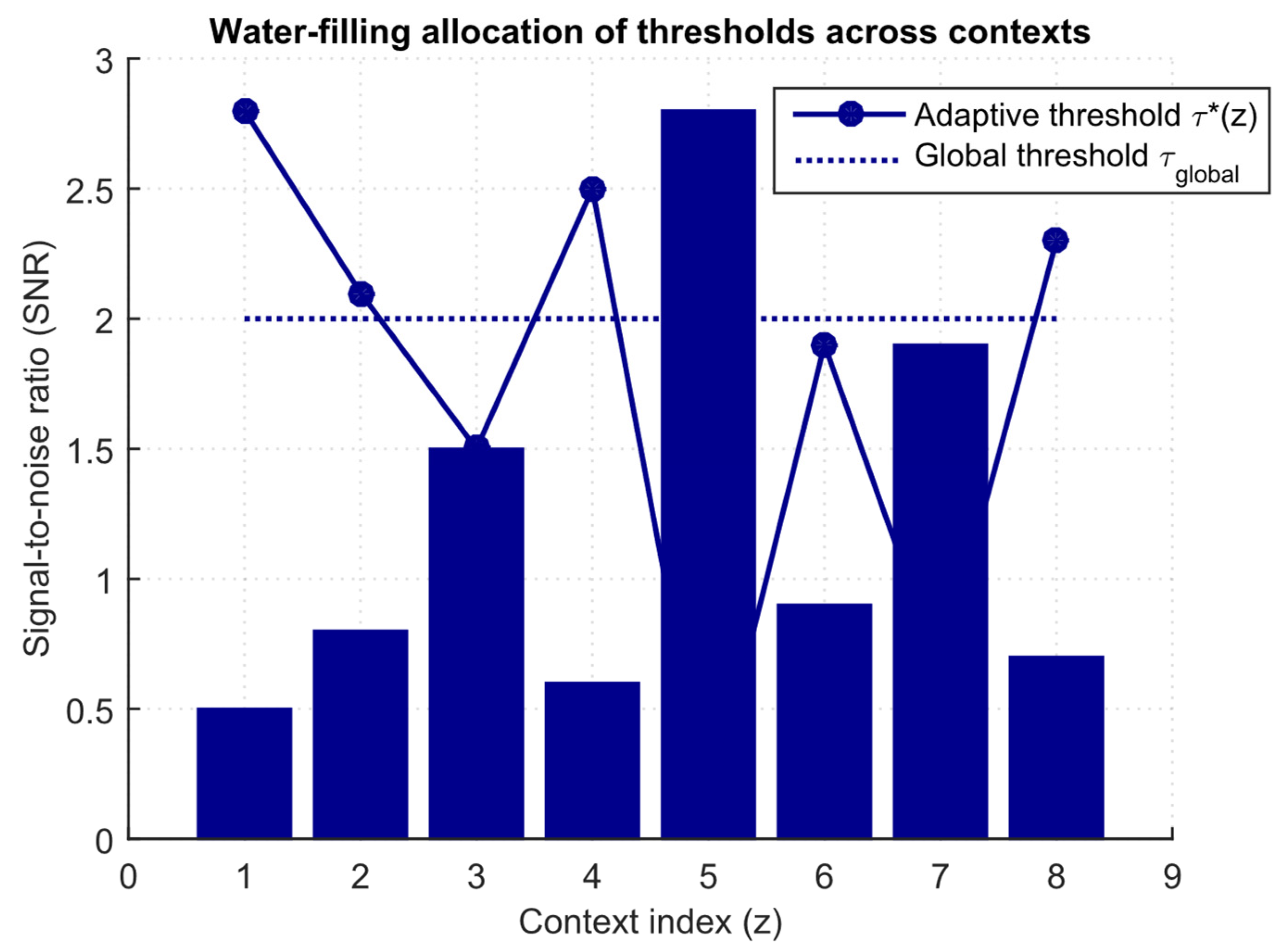
Figure 5 shows the optimal “distributive” thresholding strategy, schematically corresponding to the variational problem solution (water-filling). According to Figure 5, the sensitivity resources (TPR-budget γ) are concentrated in contexts with high separability, which actively reduces the integral FPR. It explains the statement in the text that adaptive thresholding increases the integral Chernoff coefficient and gives an exponential advantage in the minimum FPR decrease rate for large n.

Optimization with respect to τ*(z) then comes down to distributing the sensitivity budget γ over contexts z (resource allocation). To do this, the variational problem of minimizing the FPR integral under a linear constraint on the TPR integral is solved. The solution to this problem has the form of water-filling (in the Lagrange sense) as the thresholds for contexts with a “large response” (high signal-to-noise w(z)^⊤ ∙ μ_θ(z)−w(z)^⊤ ∙ μ₀(z)) become smaller, while for “noisy” contexts the threshold increases, which results in a decrease in the overall FPR.

To obtain an explicit estimate of the gain via relative entropies, it is assumed that for each z and θ, $D_{KL}\left(P_{\theta }\left(•|z\right)‖P_0\left(•|z\right)\right)=d_{\theta }\left(z\right)$. If the Kullback–Leibler divergence is higher on average over z and worst case over θ (the separability index), then for a sequential observation of size n, the asymptotically minimal FPR at fixed worst-case TPR γ behaves as

$$\underset{\min }{\mathrm{FPR}}\lesssim \exp \left(-n·\underset{\theta \in \mathsf{\Theta }}{\inf } {\mathcal{C}}_{\theta }\right),$$

(43)

where C_θ is the Chernoff term, represented as:

$${\mathcal{C}}_{\theta }=\underset{0\le s\le 1}{\max }\left(-\int \log \int p_0{\left(x|z\right)}^{1-s}·p_{\theta }{\left(x|z\right)}^{s}dxq\left(z\right)\right).$$

(44)

Context-adaptive thresholding improves the integral Chernoff term due to a better distribution of the threshold “energy” over z and therefore gives an exponential advantage in FPR performance (the lower the performance, the faster the FPR decreases with n).

To calculate π* and τ*(z), it is assumed that the space Θ is discrete or approximated by a grid {θ₁, …, θ_m}. Then the original problem is discretized as:

$$\begin{gathered} \underset{\delta }{\min }\sum _z\delta \left(x,z\right)p_0\left(x,z\right)dx \\ \mathrm{s}.\mathrm{t}. \underset{j=1\dots m}{\min }\sum _z\delta \left(x,z\right)p_{{\theta }_j}\left(x,z\right)dx\ge \gamma . \end{gathered}$$

(45)

Combining with the minimax principle, one can search for probabilities at m points π ∈ Δ^m−1, solving a convex problem:

$$\underset{\pi \in {∆}^{m-1}}{\max }\underset{\delta :R_0\left(\delta \right)\le \alpha }{\max }\sum _{j=1}^m{\pi }_j·R_{{\theta }_j}\left(\delta \right).$$

(46)

Theorem 2. 

Strict false positive reduction in informative context.

Let the space Z be discrete and finite, that is $\mathcal{Z}$ = {z₁, …, z_k}, and let the context marginal be the same under P₀ and under all P_θ, that is, q(z_i) > 0 and q_θ(z_i) = q(z_i) for all i, θ. For a fixed mixture $P_{{\pi }^{*}}$, we define two tests:

• Global test ${\delta }_{glob}\left(x,z\right)=\mathbf{1}\left\{L_{{\pi }^{\mathrm{*}}}\left(x|z\right)\ge \overline{\tau }\right\}$ with threshold $\overline{\tau }$ chosen so that $\underset{\theta }{\inf } R_{\theta }\left({\delta }_{glob}\right)\ge \gamma$ and R₀(δ_glob) = α_glob;
• The optimal context-adaptive test ${\delta }_{ctx}\left(x,z\right)=\mathbf{1}\left\{L_{{\pi }^{\mathrm{*}}}\left(x|z\right)\ge {\tau }^{\mathrm{*}}\left(z\right)\right\}$ with the threshold τ*(z) chosen such that $\underset{\theta }{\inf } R_{\theta }\left({\delta }_{ctx}\right)\ge \gamma$ and R₀(δ_ctx) = α_ctx. Then, if there exist indices i, j such that the distribution functions

  $$\begin{gathered} F_i\left(t\right)=\underset{P_{{\pi }^{*}}}{\mathrm{Pr}}\left(L_{{\pi }^{*}}\left(X|z_i\right)\le t|Z=z_i\right), \\ {F}_j\left(t\right)=\underset{P_{{\pi }^{*}}}{\mathrm{Pr}}\left(L_{{\pi }^{*}}\left(X|z_j\right)\le t|Z=z_j\right) \end{gathered}$$

  (47)

  do not coincide, and the relative “information content” ratio

  $$\exists t:{\displaystyle \frac{1-F_i\left(t\right)}{1-F_{0,i}\left(t\right)}}\ne {\displaystyle \frac{1-F_j\left(t\right)}{1-F_{0,j}\left(t\right)}},$$

  (48)

  where F_0,i is a similar cumulative distribution function under P₀, then α_ctx < α_glob, that is, with a difference in the conditional LR laws across contexts, the gain in FPR is strictly positive.

Proof of Theorem 2. 

Since Z is finite and the marginal is the same for all measures, the requirements for $\underset{\theta }{\inf } R_{\theta }$ are decomposed into a sum over z_i with weights q(z_i). Consider for a fixed z_i functions of the form:

$${\varphi }_i\left(t\right)≔{\displaystyle \frac{\underset{P_{{\pi }^{*}}}{\mathrm{Pr}}\left(L_{{\pi }^{*}}\left(X|z_i\right)\le t|Z=z_i\right)}{\underset{P_0}{\mathrm{Pr}}\left(L_{{\pi }^{*}}\left(X|z_i\right)\le t|Z=z_i\right)}}={\displaystyle \frac{1-F_i\left(t\right)}{1-F_{0,i}\left(t\right)}},$$

(49)

that is, it is the TPR to FPR ratio at a local threshold t in the z_i context. Function (49) characterizes the local threshold efficiency. For a global threshold $\overline{\tau }$, the overall (overall z) TPR and FPR are equal to the sum over i with weights q(z_i):

$$\begin{gathered} R_{{\pi }^{*}}\left({\delta }_{glob}\right)=\sum _{i}q\left(z_i\right)·\left(1-F_i\left(\overline{\tau }\right)\right), \\ {R}_0\left({\delta }_{glob}\right)=\sum _{i}q\left(z_i\right)·\left(1-F_{0,i}\left(\overline{\tau }\right)\right). \end{gathered}$$

(50)

Similarly, for the thresholds τ_i in the context set, we have sums over i. The constraint on $\underset{\theta }{\inf } R_{\theta }$ in the using $P_{{\pi }^{*}}$ turns the case into a requirement on $R_{{\pi }^{*}}$ (from the minimax argument). Also, we must have $\sum _{i}q\left(z_i\right)·\left(1-F_{0,i}\left({\tau }_i\right)\right)$ under the linear constraint $\sum _{i}q\left(z_i\right)·\left(1-F_i\left({\tau }_i\right)\right)=\mathsf{Г}$, where Γ ≥ γ is the required overall sensitivity against a mixture. It is a convex problem in the variables u_i:= 1 − F_i(τ_i) (monotonic feedback with τ_i). The solution gives a thresholding with a “sensitivity” distribution over contexts, which is equivalent to solving the Lagrange problem:

$$\underset{u_i\in \left[\mathrm{0,1}\right]}{\min }\sum _{i}q\left(z_i\right)·h_i\left(u_i\right)+\lambda ·\left(\mathsf{Г}-\sum _{i}q\left(z_i\right)·u_i\right),$$

(51)

where h_i(u_i) is the inverse coupling function h_i · (1 − F_i(τ)) = 1 − F_0,i(τ). The functions h_i are not the same, given that F_i, F_0,i are different and the optimization distributes u_i so that more u_i are allocated to contexts with greater “efficiency” (smaller hi for fixed u_i). As a result, a smaller sum $\sum _{i}q\left(z_i\right)·h_i\left(u_i\right)$ is achieved compared to an equal distribution (corresponding to the global threshold, when all ${\tau }_i=\overline{\tau }$, and u_i depend equally on the common $\overline{\tau }$). Since the functions h_i are different given the theorem condition, the optimization will strictly reduce the sum compared to the unchanged layout, which gives α_ctx < α_glob. The theorem is proved. □

Thus, the developed mathematical model reduces the problem of minimizing false alarms with guaranteed sensitivity to a minimax solution, i.e., reduces the alternatives set to a least-favourable mixture, after which it is optimal to threshold the conditional likelihood ratio. Context-adaptive thresholds give a strict benefit in an informative context. At the same time, the gain is quantitatively described through the local TPR (FPR) ratios and integral measures of distinguishability (Kullback–Leibler divergence or Chernoff coefficient). Thus, context-adaptive thresholds for IDS/IPS have been substantiated and an optimal “water-filling” sensitivity budget distribution has been derived, enabling the minimization of false positives while maintaining guaranteed sensitivity. Unlike existing approaches, a rigorous minimax formulation of the problem with a proof of its optimality is proposed.

3.2. Development of Theoretical Foundations for Ensuring the Models’ Stability Against Targeted Adjustment (Poisoning) and Adversarial Attacks

To prove the developed context-adaptive model robustness to two essential classes of adversarial influences, namely, training with targeted adjustment (poisoning, training) and test (runtime) adversarial change of objects (evasion), the same notations are adopted as in the model development itself, namely, X are features, Z is context, P₀ is a “pure” (without attack) measure, an alternative is the ${\left\{P_0\right\}}_{\theta \in \mathsf{\Theta }}$ family, and there is a mixture (prior) π for the corresponding conditional likelihood ratio $L_{\pi }\left(x|z\right)={\displaystyle \frac{p_{\pi }\left(x|z\right)}{p_0\left(x|z\right)}}$, and the detector (rule) is represented as δ(x, z) ∈ {0, 1}. At the initial stage, attack models and required guarantees are formulated.

The poisoning model (Huber-type) is that the observed “training” empirical measure $\widehat{P}$ is the “pure” ε-mixture and an arbitrary hostile measure:

$$\tilde{P}=\left(1-\epsilon \right)·P+\epsilon ·Q,$$

(52)

where Q is an arbitrary (hostile) measure, 0 ≤ ε < 1.

Often, the distortions for P₀ and for the alternatives P_θ are considered separately, that is,

$${\tilde{P}}_0=\left(1-\epsilon \right)·P_0+\epsilon ·Q_0, {\tilde{P}}_{\theta }=\left(1-\epsilon \right)·P_{\theta }+\epsilon ·Q_{\theta }.$$

(53)

The adversarial evasion model is formalized as a local data transformation in which for each initial x, the attacker can choose ^x′ from some set B(x) (e.g., a ball of radius δ in the ∥•∥ norm):

$${\mathcal{A}}_{\delta }\left(x\right)=\left\{x^{\prime }:‖x^{\prime }-x‖\le \delta \right\}.$$

(54)

The attacker chooses a strategy α—a mapping x ↦ ^x′ ∈ ${\mathcal{A}}_{\delta }$(x). Then, under P_0, there is a transformed (pushforward) measure $P_0^{\alpha }$ with density $p_0^{\alpha }\left(x^{\prime }\right)=\int p_0\left(x\right)·\mathbf{1}\left\{\alpha \left(x\right)=x^{\prime }\right\}dx$ (or, more simply, the possible distributions set {$P_0^{\alpha }$: α is admissible}).

The problem under study consists of justifying the δ detector and mathematical estimates (boundaries) design that guarantee:

• When training with contamination rate ε, the drop in sensitivity (TPR) and the increase in false alarms (FPR) are limited and correctly controlled;
• For test evasion attacks limited by the “power” δ, there is a complete (minimax) rule that ensures the given sensitivity level γ preservation and the FPR minimization in the worst-case;
• When poisoning and adversarial evasion are combined, combined assessments are given.

For this aim, the following are used: Huber-ε-contamination, Neyman–Pearson for composite hypotheses (minimax or least-favourable prior), protection through “cutting” or likelihood ratio “clipping” (clipped, censored LR—classical robust criterion), and the “robustified score” mechanism for test-time perturbations:

$$L^{-}\left(x|z\right):=\underset{{\mathit{x}}^{\prime }\in {\mathcal{A}}_{\delta }\left(x\right)}{\inf }{L}_{\pi }\left(x^{\prime }|z\right).$$

(55)

Lemma 1. 

Lemma on the mathematical expectation stabilization under distributions mixing.

Let $\tilde{P}=\left(1-\epsilon \right)·P+\epsilon ·Q$. Then for any measurable rule δ: $\mathcal{X}$ × $\mathcal{Z}$ → [0, 1],

$${\mathbb{E}}_{\tilde{P}}\left[\delta \right]=\left(1-\epsilon \right)·{\mathbb{E}}_P\left[\delta \right]+\epsilon ·{\mathbb{E}}_Q\left[\delta \right],$$

(56)

hence,

$$\left(1-\epsilon \right)·{\mathbb{E}}_P\left[\delta \right]\le {\mathbb{E}}_{\tilde{P}}\left[\delta \right]\le \left(1-\epsilon \right)·{\mathbb{E}}_P\left[\delta \right]+\epsilon .$$

(57)

In particular,

$$\left|{\mathbb{E}}_{\tilde{P}}\left[\delta \right]-{\mathbb{E}}_P\left[\delta \right]\right|\le \epsilon .$$

(58)

The lemma is proved. □

The proof of Lemma 1 yields the first conclusion that under training adjustment of the proportion ε, any risk estimate value (including FPR or TPR) shifts by at most ε in the absolute sense (and for TPR, only by a (1 − ε) factor in the worst case). It gives basic “stability”, since if ε is small, the shift is bounded.

Theorem 3. 

Resistance to poisoning in the Huber model and the optimal test form.

Let the training measures be subject to ε-contamination, that is, the recognition data obtained $\tilde{P}=\left(1-\epsilon \right)·P+\epsilon ·Q$ for all θ. Let the requirement be to ensure worst-case sensitivity $\underset{\theta }{\inf } R_{\theta }\ge \gamma$ at a minimum ${\tilde{R}}_{\theta }\left(\delta \right)={\mathbb{E}}_{{\tilde{P}}_0}\left[\delta \right]$. Then the optimal minimax rule that minimises $\underset{Q_0,Q_{\theta }}{\sup }{\tilde{R}}_0\left(\delta \right)$ given that $\underset{\theta }{\inf } \underset{Q_{\theta }}{\inf } {\mathbb{E}}_{{\tilde{P}}_{\theta }}\left[\delta \right]\ge \gamma$ is a “censored (clipped) likelihood-ratio test”, that is, a rule of the form

$${\delta }^{*}\left(x,z\right)=\left\{\begin{array}{c}1, \Lambda \left(x,z\right)>u\\ 0,\left(x,z\right)<\mathcal{\ell }, \Lambda \left(x,z\right)={\displaystyle \frac{p_{\pi }\left(x,z\right)}{p_0\left(x,z\right)}},\\ \mathrm{randomized\; on} \left[0,1\right], l\le \Lambda \left(x,z\right)\le u, \end{array}\right.$$

(59)

with suitable constants 0 < ℓ ≤ u < ∞, where π is the least-favourable prior (minimax mixture). In addition, the worst-case FPR satisfies the estimate:

$${\tilde{R}}_0\left({\delta }^{*}\right)\le R_0\left({\delta }^{*}\right)+\epsilon ,$$

(60)

and worst-case TPR satisfies

$$\underset{\theta ,Q_{\theta }}{\inf }{\mathbb{E}}_{{\tilde{P}}_{\theta }}\left[{\delta }^{*}\right]\ge \left(1-\epsilon \right)·\underset{\theta }{\inf } R_{\theta }\left({\delta }^{*}\right).$$

(61)

Proof of Theorem 3. 

Thus, the admissible alternatives are restricted via the least-favourable prior: similar to the evidence of the minimax series in your previous theorem, for an alternative families set and pollutions set, there is a “worst” mixture π* and worst pollutions $Q_0^{*}$ and $Q_{\theta }^{*}$, which form the problem saddle-point (Sion or von Neumann minimax). For the Huber model, the pollution class is convex and symmetric with respect to the linear functionals $\mathbb{E}$[δ]. Thus, the optimal adversary chooses Q concentrating the mass on those x where δ = 1 (to increase FPR) or vice versa (to decrease TPR). Then the detector problem is reduced to worst-case protection, which is formally solved by censored LRT, i.e., the classical threshold. Instead, we “limit” LR from both sides (see [42,43,47,48]); however, in this paper, the proof is a direct application of the NP argument to the L-densities set with dominated connection. The resulting estimates of the change in risk under contamination follow from Lemma 1; that is, under worst-case ${\mathbb{E}}_Q$[δ] = 1, FPR will increase by no more than ε, and TPR can decrease to (1 − ε) · R_θ(δ) under worst-case ${\mathbb{E}}_Q$[δ] = 0. The theorem is proved. □

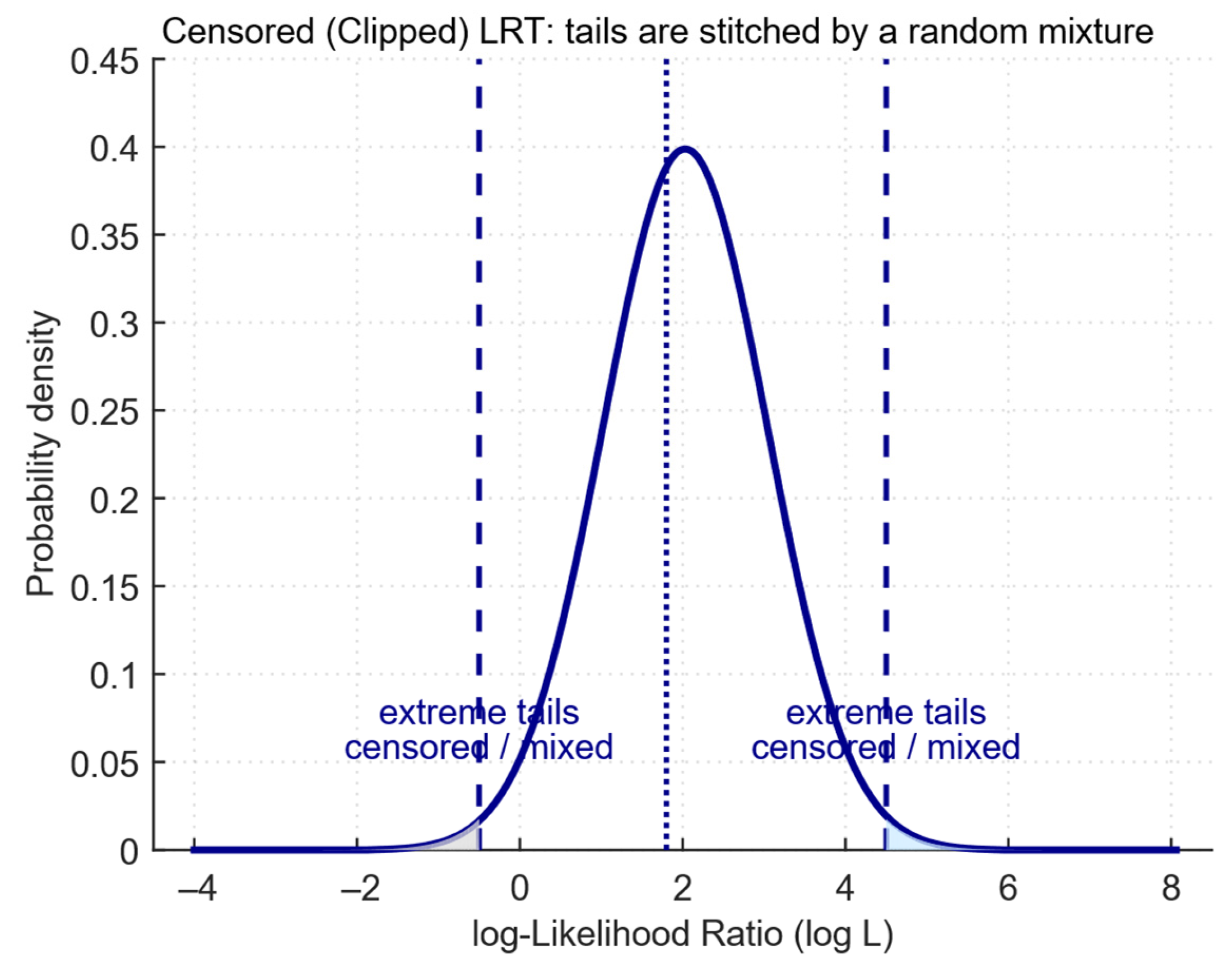
The key conclusion of Theorem 3 is that the minimax-optimal form of the test under contamination is not the usual unbounded LRT but a censored (or clipped) LRT, where the extreme LR values are “sewn up” with a random mixture. It makes the test insensitive to rare but strong poisoned points that the adversary could insert to artificially change the LRT bounds. Structurally, this corresponds to design practice, since a neural network training involves “cutting off” huge weights or responses (weight clipping) and wrapping tail estimates. At the same time, according to Lemma 1, the numerical boundaries of degradation are determined, and the thresholds are adjusted according to (59) and (60). Therefore, the aim is to ensure minimal sensitivity γ after poisoning, and it is necessary to ensure insensitivity during training:

$$\underset{\theta }{\inf } R_{\theta }\left(\delta \right)\ge {\displaystyle \frac{\gamma }{1-\epsilon }},$$

(62)

and the threshold τ (or thresholds τ(z)) should be chosen taking into account this increased required level. It gives an explicit rule for practical tuning, that is, the TPR margin is equal to ${\displaystyle \frac{1}{1-\epsilon }}$.

Next, we consider the adversarial-evasion (test-time) case of a different nature. In this context, the attacker does not change the distribution globally but individually shifts samples x → ^x′ ∈ ${\mathcal{A}}_{\delta }$(x). We formalize the worst case for a given detector δ as:

$$\begin{gathered} {FPR}^{adv}\left(\delta \right)≔\underset{\alpha \in \mathcal{A}}{\sup }{\mathbb{E}}_{X~P_0}\left[\delta \left(\alpha \left(X\right),Z\right)\right], \\ {TPR}_{\theta }^{adv}\left(\delta \right)≔\underset{\alpha \in \mathcal{A}}{\inf }{\mathbb{E}}_{X~P_{\theta }}\left[\delta \left(\alpha \left(X\right),Z\right)\right], \end{gathered}$$

(63)

where $\mathcal{A}$ is a feasible class of attacks (e.g., all measurable α with α(x) ∈ ${\mathcal{A}}_{\delta }$(x)). Thus, it is necessary to find a detector that minimizes FPR^adv subject to ${TPR}_{\theta }^{adv}\ge \gamma$. To do this, for a fixed mixture π and feasible set B(x), we define

$$L_{\pi }^{-}\left(x|z\right)≔\underset{x^{\prime }=B\left(x\right)}{\inf }{L}_{\pi }\left(x^{\prime }|z\right), L_{\pi }^{+}\left(x|z\right)≔\underset{x^{\prime }=B\left(x\right)}{\inf }{L}_{\pi }\left(x^{\prime }|z\right),$$

(64)

that is, $L_{\pi }^{-}$ is the “worst” LR that the attacker can rely on, and $L_{\pi }^{+}$ is the “best” side (used if the attacker is trying to increase TPR, which is rare). The rule

$${\delta }_{rob}\left(x,z\right)=\mathbf{1}\left\{L_{\pi }^{-}\left(x|z\right)\ge \tau \left(z\right)\right\}$$

(65)

thresholds the worst-case LR (the most conservative rate), which is natural; if even the most hostile admissible ^x′ gives LR ≥ τ, then every ^x′ will lead to a signal.

Figure 5 illustrates Theorem 3’s idea. Instead of an unlimited LRT, the optimal minimax rule under contamination censors (or clips) extreme LR values and “sews” the tails with a random mixture, which dramatically reduces the vulnerability to rare but strong poisoned points. Thus, this procedure is equivalent to the weight clipping (tail-wrapping) practice in training neural networks and formally provides a margin on TPR, so the thresholds τ (or τ(z)) must be adjusted taking this margin into account.

Figure 6 illustrates Theorem 3’s idea, since instead of an unlimited LRT, the optimal minimax rule under contamination censors (or clips) extreme LR values and “sews” the tails with a random mixture, which dramatically reduces the vulnerability to rare but strong poisoned points. Thus, this procedure is equivalent to the weight clipping practice (tail-wrapping) in training neural networks and formally provides a margin on TPR, so the thresholds τ (or τ(z)) must be adjusted taking this margin into account.

Theorem 4. 

Minimax optimality of robustified likelihood ratio under bounded perturbations.

Let B(x) be the set of admissible perturbations (e.g., a ball of radius δ in some norm), and let the attacks A class be all measurable α with α(x) ∈ B(x). Then the optimal minimax rule that minimizes $\underset{a\in \mathcal{A}}{\sup } {\mathbb{E}}_{P_0}\left[\delta \left(\alpha \left(X\right),Z\right)\right]$ subject to the constraint $\underset{\theta }{\inf } \underset{a\in \mathcal{A}}{\inf } {\mathbb{E}}_{P_{\theta }}\left[\delta \left(\alpha \left(X\right),Z\right)\right]\ge \gamma$ is chosen as a thresholding $L_{{\pi }^{*}}^{-}\left(x|z\right)$:

$${\delta }_{rob}\left(x,z\right)=\mathbf{1}\left\{L_{\pi }^{-}\left(x|z\right)\ge \tau \left(z\right)\right\}$$

(66)

Proof of Theorem 4. 

Consider a composite problem in which the hypothesis H₀: $X^{\prime }~P_0^{\alpha }$ for some α ∈ $\mathcal{A}$ (any), alternatives H₁: $X^{\prime }~P_{\theta }^{\alpha }$ for some θ ∈ Θ and the same α value, which is a classical prime vs. composite test, where “compositeness” is the α choice. In the minimax formulation, we seek a test that maximizes the worst-case TPR while constraining the worst-case FPR. Applying the general NP argument to the probability measures $\left\{P_0^{\alpha }: \alpha \in \mathcal{A}\right\}$ and $\left\{P_{\pi }^{\alpha }\right\}$ (all alternatives mix) set, we find that the optimal criterion should compare the Radon–Nikodym derivatives ${\displaystyle \frac{d{P}_{\pi }^{\alpha }}{d{P}_0^{\alpha }}}$. Since the α value is unknown, in the minimax sense, the comparison is reduced to the worst RN pairs comparison, that is, it is necessary to investigate the function:

$$\underset{\alpha }{\inf }{\displaystyle \frac{d{P}_{\pi }^{\alpha }}{d{P}_0^{\alpha }}}\left(x^{\prime }\right)=\underset{x\in \mathcal{X}:\alpha \left(x\right)={\mathit{x}}^{\prime }}{\inf }{\displaystyle \frac{p_{\pi }\left(x^{\prime }|z\right)}{p_0\left(x^{\prime }|z\right)}}=L_{\pi }^{-}\left(x|z\right)$$

(67)

which rigorous derivation requires checking dominance and measurability, but in this study, the problem of finding the supremum (infimum) by attacker parameters is solved. Therefore, the test thresholding $L_{\pi }^{-}$ is NP optimal for the worst case. The theorem is proved. □

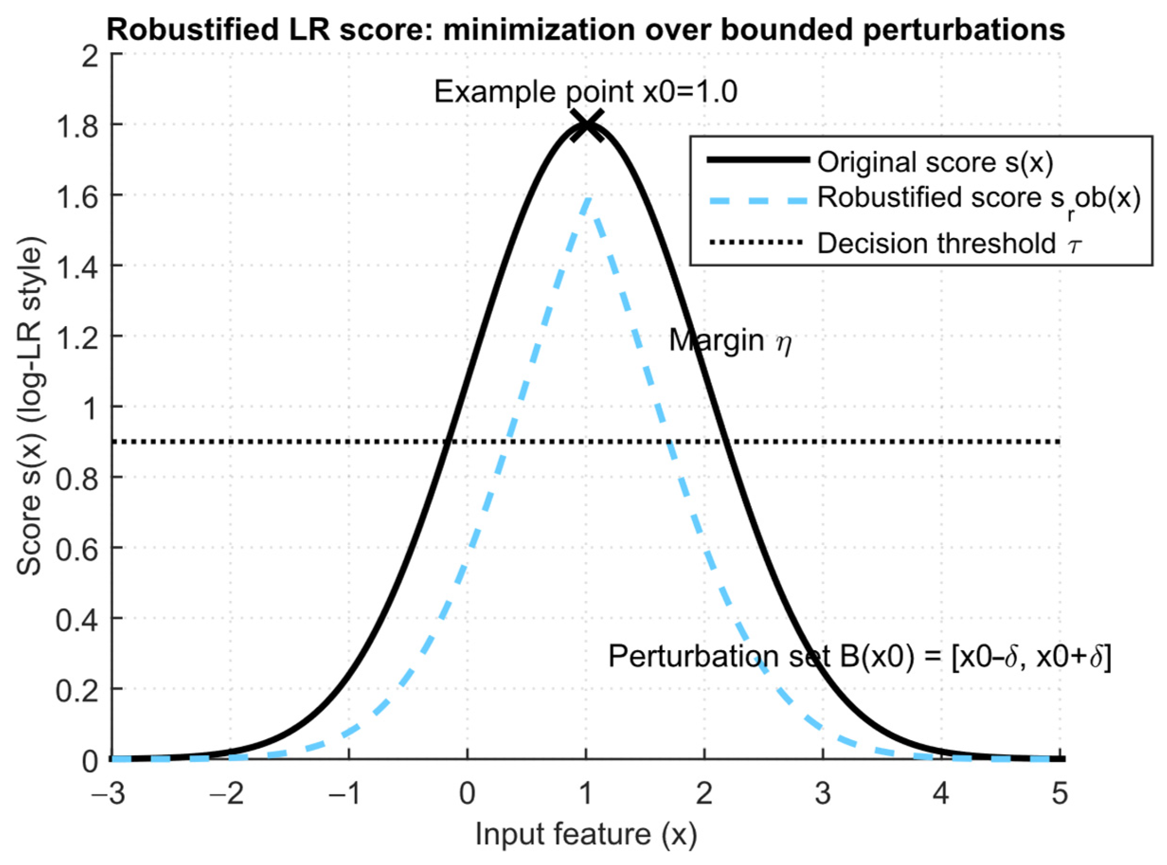
It follows from Theorem 4 that if for all x the set B(x) is compact and L_π(• ∣ z) is continuous (in x), then $L_{\pi }^{-}$ is achieved and calculated at least over the ball. In statistical practice, this is implemented as a robustified score, that is, the original score is $s\left(x\right)=\log L_{\pi }\left(x|z\right)$, but instead the calculation is performed:

$$s_{rob}\left(x\right)=\underset{‖u‖\le \delta }{\min } s\left(x+u\right),$$

(68)

and then threshold(s_rob(x)) ≥ t_s. This transformation makes the test locally invariant to evasion noise. If the original s(x) for the true “signal” was sufficiently above the threshold with a margin, then even after the worst-case perturbation, the signal will be preserved. Formally, if under P_θ for X we have:

$$\underset{P_{\theta }}{\mathrm{Pr}}\left(s\left(X\right)\ge \tau +\eta \right)\ge \gamma$$

(69)

and, at the same time, local Lipschitz insensitivity

$$\underset{‖u‖\le \delta }{\sup }\left|s\left(X+u\right)-s\left(X\right)\right|\le \eta$$

(70)

is fulfilled almost certainly, then:

$$\underset{P_{\theta }}{\mathrm{Pr}}\left(s_{rob}\left(X\right)\ge \tau \right)\ge \gamma ,$$

(71)

that is, the sensitivity preservation is guaranteed. Here, the condition with η is a quantitative margin condition: the s-values “reserve” above the threshold is greater than the possible reduction due to perturbation, which corresponds to the precise mathematical intuition of margin robustness, widely used in adversarial studies, for example, in [65,66], but in this study, it is formalized within the LR score framework.

Figure 7 shows the original LR score s(x) and its robustified version s_rob(x), defined according to (67), that is, minimizing the estimate over the feasible neighbourhood ball B(x). If an observation has a margin η above the threshold τ (margin), and local Lipschitz insensitivity holds (the possible reduction due to perturbation does not exceed η), then s_rob(x) remains above τ and the TPR is preserved, as visually seen at x₀. This diagram illustrates Theorem 4’s construction, from which thresholding the worst-case (minimized) LR yields a minimax-optimal rule against bounded perturbations.

Next, we consider combining poisoning with evasion by combining both models. The trained densities p₀ and p_π are estimated on contaminated data and are themselves used in a robustified test. Let the estimated densities after training (on ε-contaminated data) yield LR ${\widehat{L}}_{\pi }$, and let the attacker make perturbations during testing. Then, a natural robust algorithm is to train with clipping or censoring (tail limitation) and then test with $L_{\widehat{\pi }}^{-}$. Formally, if there was ε contamination during training, then by Lemma 1, the risk estimates are biased by ≤ε, and by Theorem 4, using inf-LR protects test perturbations. In sum, we obtain the worst-case FPR upper bound and the worst-case TPR lower bound:

$$\begin{gathered} {FPR}^{adv,poison}\left({\delta }^{*}\right)\le R_0\left({\delta }^{*}\right)+\epsilon , \\ \underset{\theta ,\alpha ,Q_{\theta }}{\inf }\mathbb{E}\left[{\delta }^{*}\left(\alpha \left(X\right),Z\right)\right]\ge \left(1-ϵ\right)·\underset{\theta }{\inf }\underset{\theta }{\mathrm{Pr}}\left(L_{{\pi }^{*}}^{-}\left(X|Z\right)\ge \tau \right). \end{gathered}$$

(72)

Therefore, to ensure post-attack sensitivity γ, training and stock selection must require that:

$$\underset{\theta }{\inf }\underset{\theta }{\mathrm{Pr}}\left(L_{{\pi }^{*}}^{-}\left(X|Z\right)\ge \tau \right)\ge {\displaystyle \frac{\gamma }{1-\epsilon }},$$

(73)

and, in order for the FPR to remain below a given level α in the worst case, it is sufficient to ensure during training that R₀(δ*) ≤ α − ε (if ε < α). Based on the above, it is necessary to provide a reserve ε in the thresholds and a reserve margin η for adversarial perturbations. Thus, two estimates of the impact of the attacks and conditions on guaranteed stability are obtained.

Estimate 1 

(the exact bound formula for poisoning) is that if the original detector δ has (clean) indices R₀(δ) = α₀ and $\underset{\theta }{\inf }{R}_{\theta }\left(\delta \right)={\beta }_0$, then under ε-contamination, the worst-case indices satisfy:

$${\alpha }_0\le {\tilde{R}}_0\left(\delta \right)\le {\alpha }_0+\epsilon , \left(1-\epsilon \right)·{\beta }_0\le \underset{\theta ,Q_{\theta }}{\inf }{\mathbb{E}}_{{\tilde{P}}_{\theta }}\left[\delta \right]\le {\beta }_0.$$

(74)

Therefore, in order to have $\underset{\theta ,Q_{\theta }}{\inf }{\mathbb{E}}_{{\tilde{P}}_{\theta }}\left[\delta \right]\ge \gamma$, it is sufficient (and necessary in the worst case) to demand ${\beta }_0\ge {\displaystyle \frac{\gamma }{1-\epsilon }}$.

Estimate 2 

(margin condition for adversarial robustness) is based on the assumption $s\left(x,z\right)=\log L_{\pi }\left(x|z\right)$, and let there exist η > 0 such that:

$$\underset{P_{\theta }}{\mathrm{Pr}}\left(s\left(X,Z\right)\ge \tau +\eta \right), \forall \theta \in \mathsf{\Theta },$$

(75)

and

$$\underset{x,z}{\sup }\underset{‖u‖\le \delta }{\sup }\left|s\left(x+u,z\right)-s\left(x,z\right)\right|\le \eta .$$

(76)

Then test ${\delta }_{rob}\left(x,z\right)=\mathbf{1}\left\{\underset{‖u‖\le \delta }{\min } s\left(x+u,z\right)\ge \tau \right\}$ guarantees $\underset{\theta }{\inf }\underset{\theta }{\mathrm{Pr}}\left({\delta }_{rob}=1\right)\ge \gamma$, that is, the margin condition with Lipschitz control s ensures robustness to the radius δ perturbations. If for a given X under P_θ with probability ≥ γ, there is s(X) ≥ τ + η, and perturbation reduces s by no more than η, then the minimum over the ball is still ≥τ, so the event s_rob(X) ≥ τ has probability ≥ γ. A note on the computational implementation is that the $L_{\pi }^{-}\left(x|z\right)$, practical calculation—infimum over a ball—requires significant computational effort. If s is differentiable, then the linear (first-order) worst case applies, according to which $\underset{‖u‖\le \delta }{\min } s\left(x+u\right)\approx s\left(x\right)-\delta {‖{\nabla }_{x}s\left(x\right)‖}_{*}$ (dual norm), and therefore the robustified score $\approx s\left(x\right)-\delta {‖\nabla s\left(x\right)‖}_{*}$.

Theorem 5. 

Minimax resistance to simultaneous poisoning and adversarial evasion.

Let the training measures and test objects be subject to ε-contamination and δ-bounded perturbations, respectively. The trained measures ${\tilde{P}}_0=\left(1-\epsilon \right)·P_0+\epsilon ·Q_0$ etc., and the test adversary can transform x into ^x′ ∈ B_δ(x). Let the detector be trained as a mixture (prior) π* on contaminated data using clipping or censoring (i.e., the density estimate is protected from tails), and let its testing be done using robustified LR, i.e., $\delta \left(x,z\right)=\mathbf{1}\left\{L_{{\pi }^{*}}^{-}\left(x|z\right)\ge \tau \left(z\right)\right\}$. Then there exist explicit thresholds τ(z) and margin conditions m(z) > 0, such that after any admissible contaminations and perturbations, guarantees (72) are satisfied, provided that the training offers (reserving margin):

$$\underset{\theta }{\inf }\underset{P_{\theta }}{\mathrm{Pr}}\left(s\left(X,Z\right)\ge \tau \left(z\right)+m\left(z\right)\right)\ge {\displaystyle \frac{\gamma }{1-\epsilon }},$$

(77)

and margin $m\left(z\right)\ge \underset{x\in \mathcal{X},z}{\sup }\underset{‖u‖\le \delta }{\sup }\left|s\left(x+u,z\right)-s\left(x,z\right)\right|$.

Proof of Theorem 5. 

This formulation combines Lemma 1 and Theorems 3 and 4 and does not require further modifications, since poisoning reduces the “pure” TPR to the (1 − ε) part, so the required margin is ${\displaystyle \frac{\gamma }{1-\epsilon }}$. Adversarial perturbation will reduce the score by m(z) at most, so we need a margin no less than this. With such a margin, the worst-case TPR is preserved, and the FPR will additionally increase by at most ε, so we initially need to require R₀(δ) ≤ α − ε (or equivalently, include this in the τ choice). The theorem is proved. □

Thus, criteria for resistance to poisoning and adversarial effects were developed based on the “clipped” and inf-LR tests with formal proof of minimax resistance. New estimates of FPR/TPR shifts during ε-contamination and conditions for maintaining susceptibility by introducing a margin were also obtained.

3.3. Development of a Neural Network Model for Detecting and Preventing IDS/IPS Intrusions

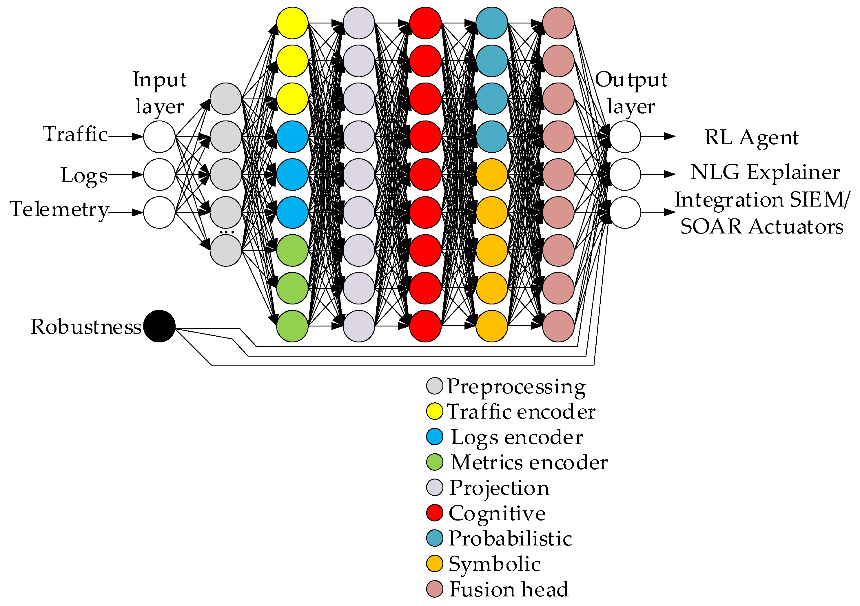
The developed theoretical foundations formed a hybrid neural network model for detecting and preventing IDS/IPS intrusion on a basic level (Figure 8), whose main features are a cognitive layer, hybrid (probabilistic-symbolic) inference, RL cycles, and operator feedback presence.

The developed neural network accepts three main classes of inputs: traffic $X^{\left(T\right)}={\left\{x_t^{\left(T\right)}\right\}}_{t=1}^T$ (packet or flow-time-series), logs $X^{\left(L\right)}={\left\{x_i^{\left(L\right)}\right\}}_{i=1}^{N_L}$ (log lines, messages), and telemetry (metrics) $X^{\left(M\right)}={\left\{x_j^{\left(M\right)}\right\}}_{j=1}^{N_M}$ (CPU, memory, sessions, attributes). Let the context Z include timestamps, subjects (IP, hosts), neural network topology G₀ = (V, E) (static), and metadata. The goal is to construct a rule δ(x, z) ∈ [0, 1] (attack speed), a priority function P: $\mathcal{S}$ → ℝ, and an explainer E(•), i.e., textual inferences.

In the preprocessing and normalization layer (deterministic), normalization and window aggregation are specified for each modal input:

$${\tilde{x}}_t^{\left(T\right)}=\underset{T}{\mathrm{Norm}}\left(x_t^{\left(T\right)}\right), {\tilde{x}}_i^{\left(L\right)}=\mathrm{T}\mathrm{o}\mathrm{k}\mathrm{E}\mathrm{m}\mathrm{b}\mathrm{e}\mathrm{d}\left(x_i^{\left(L\right)}\right), {\tilde{x}}_j^{\left(M\right)}=\underset{M}{\mathrm{Norm}}\left(x_j^{\left(M\right)}\right).$$

(78)

For traffic, we construct sliding feature vectors $f_t^{\left(T\right)}\in {\mathbb{R}}^{d_T}$ (bytes, pkts, rates, entropy, flags), for logs—token matrices $f_i^{\left(L\right)}\in {\mathbb{R}}^{\mathcal{\ell }\times d_L}$, and for metrics—vector $f_j^{\left(M\right)}\in {\mathbb{R}}^{d_M}$. The normalisation use provides stability to scale shifts:

$$\mathrm{Norm}\left(x\right)={\displaystyle \frac{x-\mu }{\sigma +\epsilon }}.$$

(79)

Layer 1 represents modal encoders with parameters ϕ_T, ϕ_L, and ϕ_M. The 1D-CNN temporal encoder with Transformer captures short-term and long-term data according to:

$$\begin{gathered} h_t^{\left(T,CNN\right)}=\underset{{\varphi }_T}{\mathrm{Conv}1\mathrm{D}}\left({\left\{f_{t-k}^{\left(T\right)}\right\}}_{k=0}^K\right), \\ {H}^{\left(T\right)}=\underset{{\varphi }_T}{\mathrm{TransEnc}}\left(h_t^{\left(T,CNN\right)}\right). \end{gathered}$$

(80)

Then, for timestep t, Transformer attention is described by the expressions:

$$\mathrm{Attn}\left(Q,K,V\right)=\mathrm{softmax}\left({\displaystyle \frac{Q·K^{\top }}{\sqrt{d}}}\right)·V,$$

(81)

where Q = W_Q · h_t, K = W_K · H, V = W_V · H.

The expressions describe a pre-trained token encoder (like BERT) with additional training:

$$H^{\left(L\right)}=\underset{{\varphi }_T}{\mathrm{TrEnc}}\left({\tilde{x}}^{\left(L\right)}\right), e_i^{\left(L\right)}=\mathrm{Pool}\left(H_i^{\left(L\right)}\right).$$

(82)

The expression describes the MLP encoder with temporal recognition:

$$H^{\left(M\right)}=\underset{{\varphi }_M}{\mathrm{MLP}}\left({\tilde{x}}_j^{\left(M\right)}\right).$$

(83)

Each modal output is projected into a common semantic space of dimension ds through linear layers according to the expressions:

$$z_t^{\left(T\right)}=W_T·H_t^{\left(T\right)}+b_T, z_i^{\left(L\right)}=W_L·e_i^{\left(L\right)}+b_L, z_j^{\left(M\right)}=W_M·H_j^{\left(M\right)}+b_M,$$

(84)

where $z^{\left(•\right)}\in {\mathbb{R}}^{d_s}$.

Layer 2 is cognitive (semantic integration, heterogeneous signals merging), whose key feature is a “sensory tokens” S = {s₁, …, s_K} (trained queries) set construction, differentiable memory M, and cross-modal attention with graph fusion. Cross-modal attention (fusion) consists of the fact that for each sensory query s_k, the following is applied:

$$a_k=\mathrm{softmax}\left({\displaystyle \frac{\left(W_Q·s_k\right)·{\left[W_K^{\left(T\right)}·Z^{\left(T\right)}‖W_K^{\left(L\right)}·Z^{\left(L\right)}‖W_K^{\left(M\right)}·Z^{\left(M\right)}\right]}^{\top }}{\sqrt{d_s}}}\right),$$

(85)

where ∥ is the concatenation over sources. A fused vector is defined as:

$${\tilde{s}}_k=a_k·{\left[W_V^{\left(T\right)}·Z^{\left(T\right)}‖W_V^{\left(L\right)}·Z^{\left(L\right)}‖W_V^{\left(M\right)}·Z^{\left(M\right)}\right]}^{\top }.$$

(86)

When introducing differentiable key-value memory (K_m, V_m), an attention update is performed at each step:

$$\alpha =\mathrm{softmax}\left({\displaystyle \frac{K_m·{\tilde{s}}_k}{\tau }}\right), V_m\leftarrow \mathrm{Update}\left(V_m,\alpha ,{\tilde{s}}_k\right).$$

(87)

The cognitive latent vector is defined as:

$$c_k=\mathrm{LayerNorm}\left(W_c·{\tilde{s}}_k+U_c·\left({\alpha }^{\top }·V_m\right)\right).$$

(88)

For contextual correlation of events, a time–entropy graph G_t = (V_t, E_t) is constructed, where $Vt$ are entities (IP, user, host, flow), and edges are weighted by the correlation coefficient ρ_uv (a co-occurrence, temporal proximity, and co-features function). Input nodes receive initial embeddings via aggregated z(•). Temporal GNN is used for this:

$$\begin{gathered} m_{u\leftarrow v}^{\left(l\right)}={\alpha }_{uv}^{\left(l\right)}·W_m^{\left(l\right)}·h_v^{\left(l\right)}, \\ {\alpha }_{uv}^{\left(l\right)}={\displaystyle \frac{1}{\sum _{\omega ϵ\mathcal{N}\left(u\right)}\exp \left(•\right)}}·\exp \left(\mathrm{SmoothReLU}\left({\alpha }^{\top }·\left[W_q·h_u^{\left(l\right)}‖W_k·h_v^{\left(l\right)}\right]\right)\right), \\ {h}_u^{\left(l+1\right)}=\sigma \left(\sum _{vϵ\mathcal{N}\left(u\right)}{m}_{u\leftarrow v}^{\left(l\right)}\right). \end{gathered}$$

(89)

It is noted that the SmoothReLU activation function is used in (89). It is the author’s modification of ReLU, presented in [67,68,69,70], defined as a linear f(x) = x for x > 0 and through a sigmoid-like smooth formula for x ≤ 0, with the parameter γ regulating the smoothing degree. In [67], it is mathematically proven that the developed ReLU modification guarantees the function at zero continuity, and the derivative on the negative half is not equal to zero, that is, the “dead neurons” vanishing gradient loop is eliminated. In practice, this means preserving the desired linear response for positive inputs (as in ReLU), but with a smooth, limited negative “tail”, which gives more stable and fast convergence and weight update in deep networks.

The cognitive layer outputs a set of contextual representations $C={\left\{c_k\right\}}_{k=1}^K$ and node embeddings $H^G=h_v^{\left(L_G\right)}$, which is a semantic picture of events and intentions.

Layer 3 is a probabilistic module of uncertainty and local hypotheses (Bayesian or generative). For robustness and uncertainty measurement, a variational approximation is introduced for latent causes u ∈ $\mathcal{U}$ (e.g., attack type, intent):

• Approximation of the posterior q_ψ(u│C, H^G) (recognition network) and the variational generator p_θ(C, H^G│u), while ELBO is represented as:

  $$\log p\left(C,H^G\right)\ge {\mathbb{E}}_{q_{\psi }}\left[\log p_{\theta }\left(C,H^G|u\right)\right]-\mathrm{K}\mathrm{L}\left(q_{\psi }·\left(u|C,H^G\right)‖p\left(u\right)\right)=L_{ELBO},$$

  (90)

  from which follows the formal optimization $\underset{\theta ,\psi }{\max }{L}_{ELBO}$;
• For classification (scoring), a posterior predictive of the type is used:

  $$s_{prob}=\mathrm{Pr}\left(\mathrm{a}\mathrm{t}\mathrm{t}\mathrm{a}\mathrm{c}\mathrm{k}|u,C,H^G\right)=\int \mathrm{Pr}\left(\mathrm{a}\mathrm{t}\mathrm{t}\mathrm{a}\mathrm{c}\mathrm{k}|u,C,H^G\right)·p\left(u|C,H^G\right)du\approx {\displaystyle \frac{1}{S}}·\sum _{r=1}^S{f}_{dec}\left(u^{\left(r\right)},C,H^G\right),$$

  (91)

  where u^(r) ∼ q_ψ.

Layer 4 is a symbolic (logical) module (differentiable symbolics). The knowledge representation in the facts and rules form, i.e., facts F = {(subj, rel, obj)}, rule R = {r_j} in the soft logic form (fuzzy or probabilistic logic). We encode the rules as differentiable predicates g_j(•) ∈ [0, 1]. We introduce soft-constraint loss:

$$L_{logic}=\sum _j{\lambda }_j·{\mathbb{E}}_{\left(C,H^G\right)}\left[\max \left(0,{\kappa }_j-g_j\left(C,H^G\right)\right)\right],$$

(92)

where κ_j is the desired compliance rate, and λ_j is the penalty. Examples of rules: “If there are many failed logins from one IP and at the same time a spike in traffic → brute-force (scan) high probability.” Each rule is implemented as a differentiable composition of predicates (neural predicates) [71]. The symbolic module produces a score s_sym ∈ [0, 1] and a symbolic output set S_facts with confidence.

Layer 5 is a hybrid inference (probabilistic with symbolic fusion). We combine the probabilistic score s_prob, symbolic s_sym, and cognitive features C. According to [72,73,74,75], we use Kalman-like fusion via Bayesian update with a neural fuser:

$$s_{fused}=\sigma \left({\omega }_p·\mathrm{logit}\left(s_{prob}\right)+{\omega }_s·\mathrm{logit}\left(s_{sym}\right)+{\omega }_c^{\top }·\mathrm{Pool}\left(C\right)+b\right),$$

(93)

or, in a more rigorous form, consider s_probs as the likelihood ratio and s_sym as the prior odds:

$$odd\left(s_{post}\right)\propto odd\left(s_{prior}\right)·LR, odd\left(s_{prior}\right)={\displaystyle \frac{s_{sym}}{1-s_{sym}}}, LR\approx {\displaystyle \frac{s_{prob}}{1-s_{prob}}},$$

(94)

and then,

$$s_{fused}={\displaystyle \frac{odd\left(s_{post}\right)}{1+odd\left(s_{post}\right)}}.$$

(95)

Layer 6 is incident prioritization (RL agent with operator feedback). The agent operates in MDP, state S_t is the summarized incident embedding ($\overline{c}$ = Pool(C)), and action a_t ∈ $\mathcal{A}$ is a priority, marking or measuring proposal. Reward r_t is formed from a combination of automatic metrics (correctness rate, FPR, TPR), operator feedback h_t ∈ {−1, 0, 1}, and business value c(•). Agent training is a policy π_θ(a ∣ S). The optimization criterion is to maximize expected cumulative reward:

$$J\left(\theta \right)={\mathbb{E}}_{\tau ~{\pi }_{\theta }}\left[\sum _{t=0}^{\infty }{\gamma }^t·r_t\right].$$

(96)

After applying the actor-critic stabilizing algorithm, the policy gradient takes the form:

$${\nabla }_{\theta }J\left(\theta \right)\approx \mathbb{E}\left[{\nabla }_{\theta }\log {\pi }_{\theta }\left(a_t|S_t\right)·{\tilde{A}}_t\right],$$

(97)

where ${\tilde{A}}_t$ is the advantage estimator (GAE). The PPO surrogate objective is represented as:

$$L^{PPO}\left(\theta \right)\approx \mathbb{E}\left[\min \left(r_t\left(\theta \right)·{\tilde{A}}_t, \mathrm{clip}\left(r_t\left(\theta \right),1-ϵ,1+ϵ\right)·{\tilde{A}}_t\right)\right],$$

(98)

where

$$r_t\left(\theta \right)={\displaystyle \frac{{\pi }_{\theta }\left(a_t|S_t\right)}{{\pi }_{{\theta }_{old}}\left(a_t|S_t\right)}}.$$

(99)

For prompt operator feedback, a human-in-the-loop reward term [76] is introduced:

$$r_t=r_t^{auto}+{\lambda }_h·r_t^{human}-{\lambda }_c·c\left(a_t\right),$$

(100)

where $r_t^{human}$ is the numerical feedback of the operator (e.g., +1 correct, −1 wrong), and λ_h balances.

Layer 7 is an explainer (NLG with contrastive justification). It takes as input a fused state $\overline{c}$, symbolic facts S_facts, RL action a, and model G to generate an explanation E:

$$E=\underset{\varphi }{\mathrm{NLG}}\left(\mathrm{t}\mathrm{e}\mathrm{m}\mathrm{p}\mathrm{l}\mathrm{a}\mathrm{t}\mathrm{e}, \overline{c}, S_{facts}, a, s_{fused}\right),$$

(101)

where NLG is a seq2seq Transformer trained with teacher forcing [77] and cross-entropy loss LNLG. For faithfulness, a faithfulness loss function is added, that is, if NLG generates a statement u, the predicate detector D is required to confirm the fact. The loss function is then represented as:

$$L_{faith}=\sum _{u\in \mathrm{g}\mathrm{e}\mathrm{n}\mathrm{e}\mathrm{r}\mathrm{a}\mathrm{t}\mathrm{e}\mathrm{d}}\mathrm{B}\mathrm{C}\mathrm{E}\left(D\left(u|C,H^G\right),1\right).$$

(102)

The system outputs are the detection (speed) s_fused, the priority $a^{*}=\arg \underset{a}{\max }{\pi }_{\theta }\left(a|\overline{c}\right)$, the facts (explanations) set E, and recommended measures R (mapping action → playbook suggestions). The overall loss function is represented as:

L_total = λ_sup · L_sup + λ_ELBO · (−L_ELBO) + λ_contr · L_contr + λ_logic · L_logic + λ_RL · L_RL + λ_NLG · L_NLG + λ_faith · L_faith + λ_reg · L_reg.

(103)

where L_sup is the supervised detection loss (binary cross-entropy), and L_contr is the contrastive self-supervised loss (InfoNCE) for modality consistency, defined as:

$$\begin{gathered} L_{sup}=\mathrm{B}\mathrm{C}\mathrm{E}\left(s_{fused},y_{label}\right)=-\left(y·\log \left(s_{fused}\right)+\left(1-y\right)·\log \left(1-s_{fused}\right)\right), \\ {L}_{contr}=-\sum _i\log {\displaystyle \frac{\exp \left(\frac{\mathrm{sim}\left(u_i,v_i\right)}{\tau }\right)}{\sum _j\exp \left(\frac{\mathrm{sim}\left(u_i,v_i\right)}{\tau }\right)}}, \end{gathered}$$

(104)

where u and v are positive pairs (e.g., flow segment and corresponding log).

Distributionally robust objective (Wasserstein-DRO) is represented as:

$$\underset{\theta }{\min }\underset{Q:W\left(Q,P\right)\le \rho }{\sup }{\mathbb{E}}_{x~Q}{\mathcal{\ell }}_{\theta }\left(x\right)\approx \underset{\theta }{\min }{\mathbb{E}}_{x~P}{\mathcal{\ell }}_{\theta }\left(x\right)+\eta ·{‖{\nabla }_x{\mathcal{\ell }}_{\theta }\left(x\right)‖}_{*},$$

(105)

that is, a first-order bound (gradient-norm regularizer) is used for robustness to evasion.

It is noted that the architecture of the developed neural network (see Figure 8) contains mechanisms of resistance to poisoning and adversarial attacks:

• Clipped weights or gradient clipping and differential privacy options are used for robust training;
• The censored LRT equivalent is implemented by limiting the points’ influence in the probabilistic layer (ELBO terms truncation for outliers), that is, formally: replace p_θ(x) with min(p_θ(x), τ_max) in the loss during training;
• DRO and gradient-norm regularizer prevent heavy dependence on small substituted sets. Mathematically, the DRO bound is represented as:

  $$\underset{Q:D_{\mathit{KL}}\left(Q‖P\right)\le \rho }{\sup }{\mathbb{E}}_Q\mathcal{\ell }\le {\mathbb{E}}_P\left[\exp \left(\lambda ·\mathcal{\ell }\right)\right]+{\displaystyle \frac{\rho }{\lambda }},$$

  (106)

  that is, moment-generating control is used.

The developed neural networks’ (see Figure 8) training should proceed in stages (see the table below), with multi-task joint fine-tuning and a human-in-the-loop RL loop. For this aim, replay buffers, prioritized experience replay (PER) for RL, and curriculum for adversarial training are used (

Table 2. The developed neural network training algorithm.

Step	Description	Aim
0	Data collection and preprocessing (balance, augmentations)	Normalization, tokenization
1	Pre-training of modal encoders ϕT, ϕL, ϕM (supervised or self-supervised)	Minimize Lsup + λcontr · Lcontr
2	Initialization of cognitive memory and GNN (batch training)	Train GNN: min∑ℓnode
3	Variational training probabilistic module (ELBO)	Maximize LELBO (reparam trick)
4	Train differentiable-symbolic module (soft rules)	Minimize Llogic (soft constraints)
5	Fusion module joint fine-tuning (multitask)
6	Adversarial or DRO fine-tune: gradient-norm reg or adversarial examples	$\mathrm{Solve} \underset{\theta }{\min } \underset{‖u‖\le \delta }{\sup }{\mathbb{E}}_{\mathcal{\ell }}\left(x+u\right)$ approximated by a gradient regularizer
7	RL-agent training with human feedback (PPO or actor-critic)	Maximize J(θ) using PPO surrogate LPPO
8	RL-agent training with human feedback (PPO or actor-critic)	Update policy with operator labels rhuman
9	Joint deployment fine-tuning (online continual training, constrained by ε-contamination bounds)	Use robust update rules, reservoir sampling, and clip updates
10	Explainability polishing (NLG) and calibration	Minimize LNLG + λfaith · Lfaith

).

According to Table 2, the following remarks are noted regarding hyperparameters and stability:

• Coefficients λ_i are selected by validation.
• To ensure resistance to poisoning, keep a stock.
• For a share ε, train so that $\underset{\theta }{\inf } R_{\theta }\ge {\displaystyle \frac{\gamma }{1-\epsilon }}$.
• The margin for adversarial η is provided through adversarial training step 6 (maximize worst-case loss inside small ball).
• For scalability, sharded memory, sparse attention for long sequences, and approximate GNN (sampling neighbours) were used.

Table 3. The developed neural networks’ main parameters.

Module (Layer)	Dimensions or Configuration (Parts)	Parameters Number	Justification
Token-embedding (logs)	vocab = 30 k × 256 (embed_dim = 256)	7.68 · 104	Universal text embedding. The number 256 is a precision (memory) trade-off for contextual log representation and NLG.
Output linear (NLG)	dmodel = 256, i.e., vocab = 30 k	7.71 · 104	Enabled for an independent decoder.
Traffic Conv1D	Conv1D: in = 32, filters = 128, k = 5; dmodel = 256	20,608	Lightweight convolution for local traffic features; small number of pairs.
Traffic Transformer	LT = 4 layers, dmodel = 256, dff = 1024	3,153,920	Four layers give a balance of speed or long memory (time patterns).
Logs Transformer	LL = 6 layers, dmodel = 256, dff = 1024	4,730,880	Deeper for text semantics (logs, messages).
Metrics MLP	16 → 128 → 256	35,200	Simple projection of metrics into a common semantic space.
Projections into semantics	3 × (256 × 256) (WT, WL, WM)	197,376	Unification of modalities in ds = 256.
Cognitive layer (fusion)	K = 32 sensory tokens (32 × 256), WQ (256 × 256), WK × 3, WV × 3, memory M = 512	926,208	Cross-modal attention with differentiable KV-memory.
GNN (event correlation)	LG = 3 × (256 × 256 W + attn. vecs.)	198,912	Graph relations: semantics translation between entities.
VAE (probabilistic module)	latent udim = 64; enc (256 → 128 → 128 → μ/logvar)	107,264	Uncertainty estimation (posterior predictive).
Symbolic module (differentiable rules)	nrules = 10 × (256 → 64 → 1 nets)	165,130	A small set of rules, differentiable (fuzzy predicates).
Fusion head (Bayesian merge)	256 → 1 (logit combination)	260	Probabilistic fusion with symbolic and cognitive.
RL: actor with critic	actor.: 256 → 256 → 8, critic.: 256 → 256 → 1	67,848/66,049	Prioritization agent (action_space ≈ 8).
NLG decoder Transformer	Ldec = 4 layers, dmodel = 256, dff = 1024	3,153,920	Compact decoder for explanation generation.
Total	–	≈28,213,575	A general average-size model that is suitable for a production cluster.

shows the developed neural network (see Figure 8) hyperparameters. It is noted that the final parameter amount is≈ 28.21 M (≈112.85 MB in fp32, ≈107.6 MB).

The choice of d_model = d_s = 256 provides O(256²) parameters in the linear layers and allows expressive encoding and combining of modalities while remaining within the “average” model size. The Transformer-layer parameters correspond to the estimate (per layer):

$$P_{transf\_layer}\approx 3·d^2+d^2+2·\left(d·d_{ff}\right)+O\left(d\right),$$

(107)

for d = 256, d_ff = 1024 gives ≈786,432 parameters/layer.

With K = 32 sensory tokens selected, the number of requests in cross-modal attention is enough to cover different “aspects” of the event but not enough to overload the memory (the parameters grow as K_d). With the selected memory size M = 512, the KV memory M × d gives 2 Md parameters, and 512 × 256 is a compromise between capacity and cost. With VAE latent u_dim = 64, it is enough for several classes of attacks (or intents), and the encoder (decoder) parameters are of the O(d · u) order. In this case, the developed neural network selected hyperparameters are as follows:

• Optimizer is AdamW, lr = 3 · 10⁻⁴ (warmup 1 k steps), weight_decay = 10⁻², which is a common combination for transformers;
• Batch size (by modality) is 256, mini-batches for sequence chunks;
• The dropout is 0.1 for the transformer, which is the layer norm. ε = 10⁻⁶;
• Gradient. Clip. Norm. is 1.0 (explosion resistance);
• Adversarial training radius δ = 0.01, …, 0.05 (in normalized features), that is, it is necessary to maintain a margin for robustness;
• Poisoning reserve ε (setting mode) = 0.01–0.05, while during training, it is essential to ensure a reserve $TPR\ge {\displaystyle \frac{\gamma }{1-\epsilon }}$;
• γ_reward = 0.99, PPO clip ε = 0.1, …, 0.2, GAE λ = 0.95, action space is 8;
• Sensory tokens K = 32; memory M = 512; transformer layers: traffic is 4, logs is 6, decoder is 4;
• d_ff = 4 · d_model = 1024, heads = 8 (by default, d_k = 32).

Thus, 256-dimensional representations have proven themselves at a high level as a “sweet spot” between expressivity and cost in monitoring systems (easy transfer between components, reasonable convergence). Transformers of 4, …, 6 layers provide a good trade-off between accuracy (latency) for tasks with slippage (logs, short-time series). Memory M = 512 and sensory K = 32 allow for storing typical patterns (scans, lateral moves) without exponential growth of parameters. RL parameters (PPO) are stable and studied in HIL (human-in-the-loop) scenarios [13,20,25,26,32].

Thus, we propose a novel hybrid neural network architecture for IDS/IPS. It combines multimodal encoders (traffic, logs, metrics), a temporal GNN for entity correlation, a variational uncertainty module, a differentiable symbolic subsystem, an RL agent for incident prioritization, and an NLG module for explanations. This provides an end-to-end pipeline of “novelty detection → active labelling → incremental supervised update” in online mode. Furthermore, the architecture formally integrates robustness mechanisms (clipped and censored LRT, DRO and gradient-norm regularization, ε reserve and η margin, and adversarial training), providing provable guarantees of protection against poisoning and evasion. This combination of functionality and formal robustness is not found in related studies.

3.4. Estimating the Developed Neural Network Model for Detecting and Preventing IDS/IPS Intrusions, Computational Costs

To estimate the developed neural network’s (see Figure 8) computational costs, d is the model dimension (d_model, d = 256 is taken), d_ff is the FFN internal size (d_ff = 1024 is taken), n_T is the traffic time window length (the tokens or steps number, n_T = 256 is taken), n_L is the length (tokens) of logs or text (n_L = 128 is taken), n_M is the metrics number (labels, n_M = 64 is taken), N = n_T + n_L + n_M is the input sequence total length (N = 448 is taken), K is the sensory queries number in the cognitive layer (K = 32 is taken), M is the KV memory size (M = 512 is taken), V is the graph nodes number (entities) (V = 100 is taken), E is the edges number in GNN (approximately E = 800 is taken), and L_gen is the generated explanation (NLG) length (L_gen = 32 is taken).

Projections Q, K, V are the three matrix multiplications 3 · n · d²; calculation of rates is Q · K^⊤; application to V ≈ 2 · n² · d (summed over all heads); output projection is n · d²; and FFN (two rulers) is 2 · n · d · d_ff, which ultimately yields:

$${FLOPs}_{transf\_layer}\left(n,d,d_{ff}\right)\approx 4·n·d^2+2·n^2·d+2·n·d·d_{ff}.$$

(108)

It is noted that in (107), only the dominant matrix operations are added, since operations like softmax, LN, and activation are small compared to matrix products and can be neglected.

Decoder-layer (masked self-attn length L_gen with cross-attn to the encoder of length N) gives:

$$\begin{gathered} {FLOPs}_{decoder\_layer}\approx \left[4·L_{gen}·d^2+2·L_{gen}^2·d+2·L_{gen}·d·d_{ff}\right]+ \\ +\left[\left(L_{gen}+2·N\right)·d^2+2·L_{gen}·N·d+L_{gen}·d^2\right], \end{gathered}$$

(109)

where the square brackets of the first term are self-attention and FFN, and the second term represents cross-attention, that is, the KV projections for the encoder and Q for the decoder, with the scores and output-projection calculation.

In cross-modal attention (cognitive layer), sensory K tokens are transformed into keys (values) for N cognitive tokens, and the main computational load falls on the projections (of the K · d² + 2 · N · d² + K · d² order for Q, K, V and the output projection) and on the attention operations themselves (of the 2 · K · N · d order). That is,

$${FLOPs}_{cross}\approx \left(2·N+2·K\right)·d^2+2·K·N·d.$$

(110)

Memory attention (K queries × M keys) is scored by applying ≈2 · K · M · d with small projections ∼ (K + M) · d². An efficient GNN (message passing) score is that if W_h is pre-computed for each vertex to avoid remultiplication for each edge, then the cost score is:

$${FLOPs}_{GNN}\approx V·d^2+E·d,$$

(111)

where the first term is the linear projections of the nodes, and the second is the aggregations along the edges.

Other modules (Conv1D, projections, VAE, symbolics, actor, critic) give obvious small O(d²) estimates per module, so their contribution has little effect on the asymptotics. The dominant behaviour is that as the sequence length n increases, the leading complexity is quadratic O(n² · d) (the attention scores term) and the linear-quadratic part O(n · d²) in the projections, so for very long n, self-attention dominates. Based on the above,

Table 4. Results of the developed neural network computational costs evaluation.

Component	Analytical Expression	FLOPs	Fraction of Total
Traffic Transformer (4 layers), n = 256	4 · (4 · n · d2 + 4 · 2 · n2 · d + 4 · 2 · n · d · dff)	939,524,096	43.36%
Logs Transformer (6 layers), n = 128	6 · 4 · (4 · n · d2 + 4 · 2 · n2 · d + 4 · 2 · n · d · dff)	654,311,424	30.20%
NLG decoder (4 layers), Lgen = 32	4 · 4 · (4 · n · d2 + 4 · 2 · n2 · d + 4 · 2 · n · d · dff)	450,887,680	20.81%
Cross-modal attention (K = 32 → N = 448)	(2 ∙ N + 2 ∙ K) ∙ d2 + 2 ∙ K ∙ N ∙ d	70,254,592	3.24%
Memory attention (K × M)	2 ∙ K ∙ M ∙ d + (K + M) ∙ d2	44,040,192	2.03%
GNN (V = 100, E = 800)	V ∙ d2 + E ∙ d	6,758,400	0.31%
Conv1D with projections	small dense ops	217,984	0.01%
VAE with small modules	small nets	200,000	0.01%
Symbolic module	fuzzy-rule nets	200,000	0.01%
Actor network (policy)	small MLP	133,120	0.01%
Critic network	small MLP	131,328	0.01%
Total (forward, batch is 1)	–	≈2.17 × 109	100%

presents the results of the developed neural network (see Figure 8) in terms of computational costs estimation.

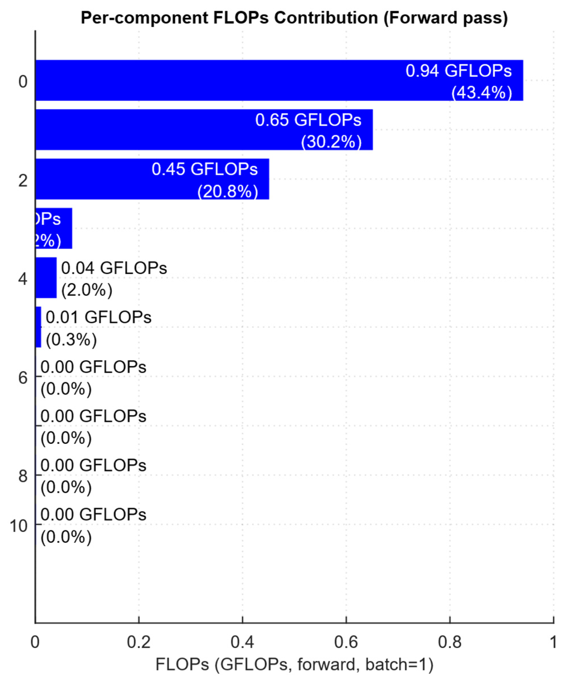
Thus, Table 4 shows each block’s contribution to the forward pass (batch is 1) total FLOPs, with the Traffic Transformer and Logs Transformer dominating, providing together ≈73% of the computational load. In comparison, the NLG decoder makes another significant contribution (~21%), and the remaining modules offer a relatively small share. Figure 9 confirms the analytical conclusion that the quadratic-in-length self-attention terms in the encoders define the main computational burden and are therefore the primary targets for optimizations (local or linear attention, reducing n or d, mixed-precision, etc.).

According to the obtained results (see Table 4 and Figure 9), the two heaviest blocks are the Traffic Transformer (considerable length n_T) and the Logs Transformer. They form the most significant part of FLOPs due to the term 2 · n² · d in (107). Decoder is substantial due to cross-attention to the long encoder.

FLOPs are converted into theoretical time. With the device (excluding memory bandwidth, synchronizations, and overhead costs), peak computing power is ideal for using time ≈ FLOPs (or peak FLOPs). For this, several benchmark peak performances (FP32) were taken, and the calculation was performed:

• NVIDIA V100 FP32 peak ≈ 15.7 × 10¹² FLOP/s;
• NVIDIA A100 FP32 peak ≈ 19.5 × 10¹² FLOP/s;
• RTX 3090 FP32 ≈ 35.6 × 10¹² FLOP/s;
• High-performance CPU FP32 ≈ 0.5 × 10¹² FLOP/s.

By denoting the forward pass theoretical time as T_f, an approximate estimate of the one complete training step (forward with backwards and optimizer) time is obtained as T_step ≈ 3 · T_f (

Table 5. Results of the time evaluation of one complete step of training.

Device	Forward FLOPs	tforward (s)	ttrain_step ≈ 3× (s)
NVIDIA V100 (FP32 peak 15.715.7 TFLOPS)	2.167 × 109	0.000138 s (≈0.138 ms)	0.000414 s (≈0.414 ms)
NVIDIA A100 (FP32 peak 19.519.5 TFLOPS)	2.167 × 109	0.000111 s (≈0.111 ms)	0.000333 s (≈0.333 ms)
RTX 3090 (FP32 peak 35.635.6 TFLOPS)	2.167 × 109	0.000061 s (≈0.061 ms)	0.000183 s (≈0.183 ms)
High-end CPU (FP32~0.5 TFLOPS)	2.167 × 109	0.00433 s (≈4.33 ms)	0.01299 s (≈13.0 ms)

).

The obtained estimates are theoretical minima, assuming fully dense execution of all operations in compute units and no memory (bandwidth) limitations and framework overheads. In practice, implementations are usually slower (often by 2…10×) due to memory bandwidth, inefficient access (communications), and overhead. With batch parallelism, B FLOPs per step scale as FLOPs_forward · B for the forward pass and about 3 · FLOPs_forward · B for full refresh (forward with backwards and opt), and the time grows almost linearly, provided that the GPU is not memory-saturated and the batch can be formed efficiently. For asymptotically dominant complexity terms, as sequence length L grows, self-attention contributes ∼O(L · d² + L² · d) (the L² · d term dominates for large L). Cross-modal fusion costs ∼O(K · N · d). It becomes insignificant relative to encoder self-attention for K ≪ N. GNN with W_h optimization in advance yields ∼O(V · d² + E · d), making dense graphs more expensive. Furthermore, storing activations in self-attention grows as O(L²) in memory and often limits the maximum L on GPUs.

Practical conclusions and recommendations for acceleration (optimization) are that if the sequence length n is large (e.g., n > 500), the dominant term of self-attention 2 · n² · d makes it necessary to switch to economical attention options (local; subquadratic; or randomized, i.e., Longformer, Linformer, or Performer, etc. [78,79,80]), which formally replace the contribution of 2 · n² · d with O(n · d · log(n)) or O(n · d), giving an asymptotic decrease in time and memory. If mixed precision (FP16 or TF32 on tensor cores) is used according to the $\propto {\displaystyle \frac{FLOPS}{peakFLOPS}}$ model, increasing peakFLOPS, real time is reduced (almost 2−8× times). With online inference, the K and V encoders’ caching sharply reduces cross-attention costs. For GNN, neighbourhood sampling (GraphSAGE) effectively reduces the number of edges E to a subgraph and linearly reduces the contribution E · d. For latency-critical inference, it is recommended to minimize the window n_T and/or the representation size d (the terms n · d · d_ff and n² · d are directly reduced), since these measures together provide a controlled trade-off between accuracy and latency by replacing quadratic terms with linearly or logarithmically growing ones and increasing hardware throughput.

Thus, a comprehensive model evaluation methodology has been developed that combines empirical benchmarking (latency, throughput, power consumption, and memory) with formal amortized computational complexity analysis and deployment cost modelling for edge and cloud infrastructures. Furthermore, a composite metric score (Cost-AUC-Latency) is proposed and validated for the first time, accounting for the trade-off between detection accuracy and computational and power costs. Hardware-adaptive optimizations (quantization, dynamic printing, and mixed-precision) that guarantee a specified service level with limited resources are described.

3.5. Development of the Virtual Neural Network System for Detecting and Preventing IDS/IPS Intrusions: Experimental Sample

To conduct the computational experiment in this study, the developed neural network (see Figure 8) was implemented as the virtual neural network system experimental sample in the MATLAB R2014b software environment. Its structural diagram is shown in Figure 10.

The developed neural network system is a modular, multi-level architecture for incident detection and prioritization tasks based on modern approaches to representing and combining heterogeneous signals. At the representation level, each modality (traffic, logs, telemetry) is encoded into a standard dimension, d-space, using specialized encoders. The key cognitive subsystem performs cross-modal attention according to (81) and differentiable KV memory, which ensures the extraction of contextually significant factors and the aggregation of information into K “sensory” vectors. In parallel, a graph correlation of events is built, which encodes spatio-temporal dependencies between network entities and allows approximating cause-and-effect and latent relations in the data.

The developed neural network systems’ second component is a hybrid inference, which is a stochastic (variational) module with a latent variable u that implements the posterior distribution q_ψ ∙ (u│C, H^G) and optimizes L_ELBO, which provides a reasonable uncertainty estimate and the predictive score s_prob. The symbolic module specifies soft logical predicates g_j ∈ [0, 1] and penalties L_logic, allowing expert rules embedding. The probabilistic and symbolic signals combination is performed according to Bayesian logic through the posterior odds odds_post ∝ odds_prior · LR, which formalizes the trade-off between data and knowledge.

The developed neural network systems’ third component is decision making and adaptation, and the prioritization agent is trained in MDP with the objective function $J\left(\theta \right)={\mathbb{E}}_{\tau ~{\pi }_{\theta }}\sum _t{\gamma }^t·r_t$, where rt includes automatic metrics and operator feedback. It ensures human-in-the-loop policy correction and dynamic re-evaluation of incidents. For reliability, robustness mechanisms are built in: censored (robustified) LR and DRO regularization (gradient norms) protect against poisoning and adversarial attacks, and margin conditions and contamination reserve ε formalize the requirements for maintaining TPR under data degradation.

Thus, a representative virtualized experimental setup “virtual neural network system” has been developed. It combines parameterizable attack playbooks, realistically generated (GAN and flow-based) and real traffic, hardware-in-the-loop emulation, and containerized deployment, providing a reproducible platform for in-depth testing of IDS/IPS detection and resilience. Furthermore, for the first time, a protocol for the experimental setup has been formalized with automated annotation, a shadow mode, and a composite evaluation metric (Cost-AUC-Latency with robustness), allowing for simultaneous consideration of detection quality, latency, and computational and energy costs.

4. Case Study

This section presents an applied study, including the input datasets’ creation and preprocessing with synchronized traffic time series, logs, and metrics; attack simulations (including DDoS); the input datasets’ homogeneity and representativeness verification using clustering methods (k-means); and partitioning into training, validation, and test subdatasets to reduce bias. The aim of these stages is to ensure that the data reflects real subgroups and rare classes, ensuring statistically significant and generalizable results. To validate the developed neural network architecture, a multi-level metrics system was used, within which framework the following metrics were obtained, namely, ROC AUC (ranking discrimination), precision (alert purity), recall and TPR (real attacks coverage), F1 (precision-recall trade-off for unbalanced classes), and FPR (false alarm rate affecting the SOC load). Detection latency metrics (median or p95), which serve as a measure of response time, computational scalability and cost metrics (throughput, GFLOPs, CPU, GPU, and RAM utilization), and confidence estimate calibration (ECE) were also defined. The Cost-AUC-Latency composite metric reflects the practical trade-off between detection quality, latency, and operational costs. Robustness was assessed through stress tests with feature drift and ε-contamination (poisoning modelling), where TPR degradation and FPR changes were recorded to quantify the DRO robustness and effectiveness, clipping, and prioritized replay methods during incremental learning. Practical and legal suitability are also demonstrated by measuring the time it takes to prepare evidence packages, the correctly generated artifact proportion, and the chain-of-custody (hashes, signatures) completeness, which ensures not only detection but also the systems’ operational and legal applicability in SOCs and when interacting with law enforcement agencies.

4.1. Formation, Analysis, and Pre-Processing of the Input Dataset

To conduct the computational experiment, an input dataset was formed (Figure 11), consisting of two time series of network traffic measurements (in bytes per second, i.e., bytes/s), according to which “clean” traffic data and data with a built-in (simulated) DDoS attack were distinguished. The dataset covers the period from ~00:00 to ~10:00 on 7 September 2024. It contains normal load fluctuations of about ~900, …, 1400 bytes/s and one artificial burst of traffic in the approximate interval of 06:20, …, 07:10 with a peak of about 6000, …, 7000 bytes/s.

Figure 11 shows a time series of network traffic with low-amplitude daily variability and sensor noise, superimposed by a simulated DDoS attack that causes a pronounced volumetric spike in the 400, …, 460 index range. It is noted that in Figure 11, the “blue curve” shows the traffic with the injected simulated attack (DDoS-like volumetric spike), and the “red curve” shows the clean data (baseline) without the attack. The DDoS attack increases the byte rate and packet rate per second, while simultaneously increasing the unique source IP addresses and the number of failed authentication attempts, thus forming a multimodal signal suitable for validating both signature-based and anomaly-based IDS/IPS detection methods. The main experimental dataset was compiled by the authors: synchronized time series of network traffic, system logs, and telemetry with an embedded (simulated) DDoS attack; the amount is 600 records with a resolution of 1 min (≈00:00, …, ≈10:00 9 July 2024); and the attack occupies indices ~400, …, 460 (≈10% of observations). Based on Figure 11,

Table 6. The input dataset.

Title 1	Type	Unit	Short Description	Count	Mean	Std	Min	25%	50%	75%	Max
bytes_clean	float	bytes/s	Baseline bytes per second (no attack)	600	1141.39	97.21	853.88	1076.65	1141.92	1204.61	1466.36
bytes_attack	float	bytes/s	Bytes per second with the injected attack scenario	600	1429.44	1036.52	853.88	1080.64	1150.69	1224.96	7038.22
pkts_attack	float	packets/s	Packets per second with the injected attack scenario	600	138.79	53.09	68.55	109.27	134.31	147.29	401.14
unique_src_ips_attack	int	count	Unique source IPs observed (attack scenario)	600	15.78	37.98	3	4	4	4	202
failed_logins_attack	float	count	Failed login attempts (attack scenario)	600	0.465	0.851	0.102	0.167	0.201	0.240	4.21
cpu_percent_attack	float	%	CPU utilization percent (attack scenario)	600	21.62	5.91	12.62	17.11	21.01	24.29	46.16

presents the input dataset with network traffic, logs, and telemetry characteristics, including both clean data and simulated attacks for subsequent training and testing of the IDS/IPS model.

Table 6 contains 600 rows, each corresponding to a minute of network activity observation, and eight columns with features. The columns include a timestamp, normalized network traffic without attacks (bytes_clean), traffic with an injected attack (bytes_attack), packets per second (pkts_attack), the unique source IP addresses number (unique_src_ips_attack), the failed logins number (failed_logins_attack), the CPU load in percent (cpu_percent_attack), and a binary label reflecting whether the record belongs to the “clean data” or “attack” class. The period from the 400th to the 460th row shows characteristic anomalies: a sharp increase in traffic amount, the number of packets, unique sources, and failed logins, which corresponds to the simulated distributed attack scenario.

For each modal input, a deterministic preprocessing layer is applied, consisting of normalization and aggregation over a sliding window. Sliding vector features (bytes, pkts, rates, entropy, flags, etc.) are generated for traffic, tokenization and token matrix generation are applied for logs, and vector representations are used for metrics. Standardization (normalization) is performed using the scaling formula [81] for each feature.

To assess the input dataset homogeneity, the Levene test (W) (robust test for the variances equality, centred on the median), Bartlett’s test (χ²) (sensitivity to normality), Kolmogorov–Smirnov two-sample test (D_n,m) (distributions equality test), Mann–Whitney test (U) (nonparametric test for shift in medians or location, standard U-statistics), and Cohen’s test (effect size estimate for the mean difference, pooled standard deviation) were used [81,82,83,84,85]:

$$\begin{gathered} W={\displaystyle \frac{\left(N-k\right)·\sum _{j=1}^k{n}_j·{\left({\overline{Z}}_{j•}-{\overline{Z}}_{j••}\right)}^2}{\left(k-1\right)·\sum _{j=1}^k\sum _{i=1}^{n_j}{\left(Z_{ij}-{\overline{Z}}_{j•}\right)}^2}}, \\ {\chi }^2={\displaystyle \frac{\left(N-k\right)·\ln \left(S_p^2\right)-\sum _{j=1}^k\left(n_j-1\right)·\ln \left(S_j^2\right)}{1+\frac{1}{3·\left(k-1\right)}·\left(\sum _{j=1}^k\frac{1}{n_j-1}-\frac{1}{N-k}\right)}}, \\ {D}_{n,m}=\underset{x}{\sup }\left|F_n\left(x\right)-G_m\left(x\right)\right|, d={\displaystyle \frac{{\overline{x}}_{attack}-{\overline{x}}_{clear}}{s_{pooled}}}, \\ {s}_{pooled}=\sqrt{{\displaystyle \frac{\left(n_1-1\right)·s_1^2+\left(n_2-1\right)·s_2^2}{n_1+n_2-2}}}, \end{gathered}$$

(112)

where $Z_{ij}=\left|X_{ij}-{\tilde{X}}_j\right|$ differences from the median in the j-th group, k is the number of groups (in this dataset, there are 2: “clean” and “attack”), $N=\sum n_j$, $S_j^2$ is the sample variance in the j-th group, $S_p^2$ is the pooled variance, and F_n and G_m are the empirical distribution functions of two samples.

Table 7. Results of input dataset homogeneity evaluation.

Feature	n_Clean	n_Attack	mean_Clean	mean_Attack	var_Clean	var_Attack	var_Ratio	Levene_Stat	Levene_p	Bartlett_Stat	Bartlett_p	KS_Stat	KS_p	MannW_Stat	MannW_p	Cohens_d
bytes_attack	540	60	1136.876	4062.497	9549.6	3 · 106	312.7	1376.5	0	1719.1	0	0.95	0	473	0	5.313
pkts_attack	540	60	125.636	257.17	548.89	7764	14.15	410.19	0	339.03	0	0.811	0	2696	0	3.704
unique_src_ips_attack	540	60	4.013	121.717	0.306	1962.2	6413.4	1079.6	0	3321.8	0	1.0	0	0	0	8.453
failed_logins_attack	540	60	0.196	2.883	0.0016	0.722	462.3	1477.1	0	1923.1	0	1.0	0	0	0	9.971
cpu_percent_attack	540	60	20.121	35.092	13.6	25.3	1.86	11.59	0.0007	12.095	0.0005	0.98	0	15	0	3.897

shows the homogeneity assessment results (clean and attack segments). Table 7 shows for each variable the observations of i number of n each group, means and variances, variance ratios, statistics, and p-values of the Levene, Bartlett, Kolmogorov–Smirnov, Mann–Whitney, and Cowan tests.

The input dataset homogeneity assessment results (Table 7) show a discrepancy in the distributions and dispersions between the “clean” and “attacked” segments for all the considered features: small p-values in the Levene and Bartlett tests confirm significant heterogeneity of variances (especially for bytes, pkts, unique_src_ips, and failed_logins), and KS and Mann–Whitney indicate statistically significant differences in the distribution shapes and central tendencies. According to Cohen’s d-test, they are observed for the features failed_logins and unique_src_ips (d ≫ 3), which reflects a strong shift in behaviour during the attack, while bytes and pkts also show large effects, but with a large dispersion in the attack segment. Therefore, the dataset is clearly heterogeneous between the “clean” and “attack” states, which makes the detection task statistically feasible. Still, the high variance of attack signals (and broad tails) requires robust methods (robust estimation, regularization, DRO) when training models to avoid overfitting on extreme examples.

The input dataset representativeness was assessed (see Figure 11 and Table 6) using the k-means method, according to which the k-means objective (intra-cluster variance minimization) [86,87,88,89] is calculated as:

$$J\left({\left\{C_j\right\}}_{j=1}^k\right)=\sum _{j=1}^k\sum _{x_i\in C_j}{‖x_i-{\mu }_j‖}^2\to \underset{\left\{C_j\right\},\left\{{\mu }_j\right\}}{\min },$$

(113)

where ${\mu }_j={\displaystyle \frac{1}{\left|C_j\right|}}·\sum _{x_i\in C_j}{x}_i$ is the centre of the j-th cluster.

The silhouette value for the i-th element is defined as:

$$S\left(i\right)={\displaystyle \frac{b\left(i\right)-a\left(i\right)}{\max \left\{a\left(i\right),b\left(i\right)\right\}}},$$

(114)

where

$$\begin{gathered} a\left(i\right)={\displaystyle \frac{1}{\left(C_{p\left(i\right)}-1\right)}}·\sum _{x_j\in C_{p\left(i\right)},j\ne i}d\left(i,j\right), \\ b\left(i\right)=\underset{q\ne p\left(i\right)}{\min }{\displaystyle \frac{1}{\left|C_q\right|}}·\sum _{x_j\in C_q}d\left(i,j\right), \end{gathered}$$

(115)

where p(i) is the cluster index of the i-th point, and d(•, •) is the chosen metric (the Euclidean metric is accepted [86,88,89]). The average silhouette score for all points gives the clustering quality −1 ≤ $\overline{s}$ ≤ 1.

The k-means inertia, which is the internal total squared error used in elbow analysis, is defined as [86]:

$$inertia=\sum _{j=1}^k\sum _{x_i\in C_j}{‖x_i-{\mu }_j‖}^2.$$

(116)

Standardization before clustering consists of the following: for each feature f [86,87]:

$$\tilde{f}={\displaystyle \frac{f-\overline{f}}{s_f}},$$

(117)

so that the feature scales do not dominate.

The results of k-means for k = 2 in the “clean” data and “attack” data interpretation are given in

Table 8. Results of assessing the input dataset representativeness using the k-means method.

Cluster	Size	Mean_Bytes (Bytes/s)	Mean_Pkts (Pkt/s)	Mean_Unique_Srcs (Count)	Mean_Failed_Logins	Mean_Cpu_Percent	Silhouette_Mean
0 (clean)	540	1136.88	125.64	4	0.196	20.12	≈0.62
1 (attack)	60	4062.50	257.17	122	2.883	35.09	≈0.85
Total	600	–	–	–	—	—	average ≈ 0.65

.

Figure 12, Figure 13 and Figure 14 show the graphical results of assessing the representativeness of the input dataset using the k-means method. Figure 12 shows the PCA projection, Figure 13 shows the time series with bytes coloured by cluster, and Figure 14 shows the elbow diagram (inertia) and silhouette diagram.

The PCA projection (Figure 12) shows a clear separation of the two groups, where the large dense cloud mass corresponds to regular traffic, and a separate compact cluster (attack) is removed in the PCA-1 direction (the bytes and unique_srcs features contribution). The high density and remoteness of the attack cluster confirm the anomalous mode’s unambiguous representativeness, which also explains the high average silhouette for this cluster (~0.85). A purely distinguishable cluster means the presence of a simple method (e.g., cluster- or threshold-based) has a basis for primary detection.

The time diagram, where the points from the attack interval are coloured in the “attack” cluster colour (Figure 13), demonstrates that the clustering is consistent in time, namely, almost all “attack” labels are concentrated within a predefined interval (indices 400, …, 460). It confirms the cluster’s high temporal coherence and indicates that the dataset is representative of both normal and abnormal modes in the temporal correlation of event context. In addition, a gradual ramp-up or ramp-down is observed within the attack interval, which models a realistic DDoS profile rather than spike noise.

The elbow curve (Figure 14a) shows a sharp decrease in inertia from k = 1 to k = 2 and much smaller decreases thereafter—a classic clue that k = 2 is sufficient. The silhouette diagram (Figure 14b) confirms this choice, as the silhouette maximum occurs at or near k = 2, which represents the best trade-off between cluster compactness and separability. Together, these plots provide an objective basis for choosing k = 2 to distinguish between “clean” and “attack” states in this dataset.

Table 9. Results of partitioning data into two clusters using the k-means method.

Metric	Cluster 0 (Clean)	Cluster 1 (Attack)	Interpretation
size	540	60	An attack that is ≈10% of the epoch is a realistic, rare anomaly
mean bytes (bytes/s)	1136.88	4062.50	Substantial volumetric shift (×≈3.6)
mean pkts (pkt/s)	125.64	257.17	Packet rate grows (~×2)
mean unique_srcs	4	122	An attack introduces many source IPs (DDoS)
mean failed_logins	0.196	2.883	Elevated login failures (brute-force signature)
mean cpu %	20.12	35.09	Increased server load during the attack
silhouette (cluster mean)	≈0.62	≈0.85	Clusters are well separable (esp. attack)

presents the results of splitting the data into two clusters using the k-means method, indicating each cluster size, average values for key features (bytes, pkts, unique_srcs, failed_logins, CPU), and average silhouette estimates for assessing the clusters’ representativeness and separability (clean vs. attack).

Table 9 shows that k-means clustering identified two clearly distinguishable states: a large “clean” cluster (540 observations) with an average traffic amount of ≈1136.9 bytes/s and a minor “attack” cluster (60 observations, ≈10%) with a sharply increased traffic of ≈4062.5 bytes/s, a higher source number (≈122 vs. 4), and a higher failed login number (≈2.88 vs. 0.20). High mean silhouette values (≈0.85 for “attack” and ≈0.62 for “clean”) together with significant differences in means indicate a strong signal of separability between the anomaly modes and compactness in the feature space. In practice, this means high attack detectability in this dataset but also indicates an imbalance (attacks are a low percentage), requiring stratified sampling or class correction methods in model training.

To determine the training, validation, and test datasets sizes (taking into account Big Data), it is recommended to maintain the splitting standard proportions: the datasets “Train”, “Validation”, and “Test” are 80%, 10%, and 10%, respectively, taking into account the attacks share (in this example, attack is ≈10%). For illustration, in the “conservative” Big Data version with a total amount of 107 records, we get “Train” is 8106 (≈80%, including ≈ 8106 attack samples), “Validation” is 106, and “Test” is 106. In the large-scale version with 108 records, we get “Train” is 8107, “Validation” is 107, and “Test” is 107. This distribution ensures sufficient representation of rare attacks in the validation and test datasets for a stable assessment of metrics (FPR, TPR, and AUC) with low variance. For very low attack rates (<1%), it is necessary to apply stratified partitioning or balancing methods (oversampling or data augmentation) in the training dataset and ensure the attack’s presence in the validation or test for the final estimates, correct validation, and representativeness.

4.2. Results of the Developed Neural Network Training Effectiveness Evaluation

The training process is implemented as a multi-stage protocol, including modal data collection and preprocessing with sliding-window aggregation, subsequent pretraining of modal encoders in supervised and self-supervised modes, initialization of the cognitive memory and graph neural network, and variational optimization using the ELBO criterion for latent representations. The next stage involves training a differentiable symbolic block and jointly fine-tuning the modal fusion mechanism. To improve model robustness, adversarial and distributionally robust fine-tuning is performed, followed by training the RL component using the PPO algorithm and a human-in-the-loop model to generate optimal response strategies. The final stages include the systems’ joint deployment with online retraining on streaming data, calibration, and the explainable NLG inferences’ generation. The model architecture is characterized by the following parameters: d_model = 256, d_ff = 1024, four Traffic Transformer layers, six Logs Transformer layers, four NLG decoder layers, 32 sensor tokens, a 512-dimensional KV memory, a three-layer GNN, and a 64-dimensional VAE latent space, which in total amounts to about 28.2 million parameters. For optimization, the Adam algorithm is used with initial parameters, training rate is 3 · 10⁻⁴ warmup of 1000 steps, weight_decay = 1 · 10⁻², batch size is 256, dropout is 0.1, ε (LayerNorm) = 10⁻⁶, and gradient_clip_norm is 1.0. Robustness is achieved by using adversarial perturbations with radius δ ≈ 0.01, …, 0.05, poison reserve ε = 0.01, …, 0.05, and PPO with γ = 0.99, clip = 0.1, …, 0.2, and GAE λ = 0.95; additional gradient norm regularization, DRO, and curriculum (adversarial) replay strategy are used if necessary.

During the development of the neural network (see Figure 8) training, stable classification indicators were obtained, shown in Figure 15, Figure 16, Figure 17, Figure 18, Figure 19, Figure 20 and Figure 21. The validation ROC AUC increased to approximately 0.94, …, 0.96, and precision, recall, and F1-score during validation stabilized in the 0.90, …, 0.96 region, demonstrating high ranking quality and a balance between false positives and misses. The developed neural network allowed us to simultaneously reduce the FPR to a single percent while maintaining a low FNR. At the same time, the built-in concept-drift detector reliably recorded two significant distribution changes and allowed incremental updates to be initiated. It is noted that the RL-based incident prioritization module showed a steady increase in average rewards after operator feedback, confirming the human-in-the-loop effectiveness for accelerated policy fine-tuning.

According to Figure 15, the training loss curve decreases monotonically with noise, confirming the optimization convergence on the training dataset (initial decrease from ≈1.2 to ≈0.05). The validation loss generally follows the training loss. Still, at ≈60th epoch, there is a noticeable spike followed by wave-like dynamics, which is a typical sign of overfitting and/or concept drift in the validation data. At the same time, slight stochasticity and irregular local increases are most likely due to augmentations, batch noise, and episodic adversarial fine-tuning.

The early stopping implementation (Figure 16) prevents further overfitting. The model was stopped at the validation performance peak (early stopping), which keeps the validation loss low and reduces the gap with the training loss. The drift monitoring mechanism recorded a change in the distribution around the 62nd epoch, after which an adaptation (incremental update) was performed, which quickly restored and even improved the validation without long-term overfitting.

Figure 17 shows the AUC value dynamics on the validation dataset by training epochs, showing a steady improvement in ranking quality to ≈0.94, …, 0.96, with a short-term drop in the 62, …, 70th epochs region (adversarial effect or concept drift) and subsequent recovery after adaptation measures.

According to Figure 17, the ROC AUC increases from ≈0.60 to ≈0.94–0.96 as training progresses, indicating a steady improvement in the model’s ability to rank signal against noise during validation. There is a noticeable short-term dip in AUC of ~0.04 around epoch ≈ 62, …, 70, coinciding with the adversarial fine-tuning phase and demonstrating the model’s sensitivity to targeted perturbations. After this, the AUC partially recovers, indicating either that subsequent fine-tuning (robust training) partially corrects the degradation or that thresholds are adjusted and the system is calibrated.

According to Figure 18, the precision and recall values improve approximately synchronously (precision ≈ 0.95, recall ≈ 0.94), and F1 follows the same dynamics, which is a sign of a well-balanced classifier after threshold tuning. In the ≈40, …, 85 epochs interval, there are local fluctuations, where in some segments, precision grows more strongly than recall, which indicates a shift in threshold optimization in reducing false positives (an obvious trade-off). At the same time, short-term recall dips (around the 70th–80th epoch) correlate with drift (attacks) spikes on other metrics, showing the temporary loss of ability to catch some attacks.

Figure 19 shows the positive and false negative dynamics during training, where at the marked “burst” moments, sharp jumps in FPR and FNR caused by attacks are observed, which allows us to evaluate the developed neural network’s (see Figure 7) stability to abnormal loads.

According to Figure 19, FPR generally decreases steadily to low values (~0.01, …, 0.03), indicating the false alarm mitigation measures’ effectiveness (e.g., censored-LR, contextual thresholds). At the same time, sharp local jumps in FPR are observed at the “burst” episodes ≈ 25, 50, and 78, which is a typical effect of mass scans (noise) bursts or targeted false alarm provocations. FNR also has a general downward trend but shows short-term increases in the same burst windows, reflecting the trade-off between FPR and FNR during anomalies and emphasizing the need for adaptive thresholds and filtering during bursts.

Figure 20 shows the changes in drift statistics over time, with the threshold exceedance moments marked, which indicate recorded concept drift events and the need to adapt the model to the changed data distribution.

In Figure 20, the base drift statistic value is stable at ≈0.02, …, 0.04, but two distinct spikes are visible at ≈60, …, 80 and ≈130, …, 140, which exceed the 0.08 chosen threshold, indicating clear concept drift events. The dots marked with crosses are concentrated at these spikes’ beginning and end, indicating that the detector detects an entry into drift and then a gradual return to a new regime. These nature patterns are typical for attack campaigns or changes in traffic profile (seasonality, change of applications) and require prompt monitoring, incremental model updates, and a retraining (buffering) strategy for new data.

Figure 21 shows the changes in actual positive rate (TPR) over time and the use of labelled samples moments for incremental update, demonstrating the accuracy restoration after concept drift due to adaptation updates.

According to Figure 21, the base TPR gradually increases with data accumulation (from ≈0.60 to ≈0.86), but at concept change around ≈70 and ≈150, TPR drops by ~0.15–0.20, which is a typical manifestation of distribution change. After two adaptation updates (≈75 s with ~400 labelled examples and ≈155 s with ~1200 examples), TPR quickly restores and even exceeds previous values, demonstrating the incremental labelling effectiveness. The “reserve” logic is obvious, since a larger update gives a stronger and longer-lasting increase in TPR but requires significant costs for labelling and data buffer planning (prioritization).

Figure 22 shows the changes in the agent’s reward function over training episodes, where the vertical bars correspond to operator interventions that lead to local reward growth and accelerated improvement of the incident prioritization strategy.

As shown in Figure 22, the reward curve shows a slow but steady improvement in the prioritization policy (the moving average increases from negative (or zero) values to ≈0.5, …, 0.58), and the vertical markers of human feedback events coincide with sharp jumps in reward, confirming that human-in-the-loop effectively accelerates training. After each feedback phase, the agent is fixed at a higher reward level, although fluctuations remain, which is an expected effect in the SOC stochastic and complex environment.

Table 10. Results of comparative analysis of neural network architectures.

Architecture	Validation ROC AUC	Precision	Recall	F1-Score	FPR	FNR
MLP (baseline)	0.89	0.87	0.85	0.86	0.07	0.08
CNN	0.91	0.89	0.87	0.88	0.06	0.07
LSTM	0.92	0.90	0.89	0.89	0.05	0.06
Autoencoder-based IDS	0.88	0.84	0.86	0.85	0.08	0.09
Transformer	0.93	0.90	0.88	0.91	0.06	0.05
Temporal Graph Network	0.92	0.88	0.91	0.91	0.04	0.05
EvolveGCN	0.91	0.88	0.85	0.87	0.07	0.06
Graph Transformer	0.94	0.91	0.89	0.91	0.05	0.05
Developed a neural network	0.96	0.95	0.94	0.95	0.03	0.04

presents the comparative analysis results of the developed neural network (see Figure 8) and several popular architectures used for intrusion detection and prevention (IDS/IPS) tasks. In particular, MLP is used as a base classifier for processing network features [17], CNN is used to extract local patterns in network flows [27], and LSTM takes into account the temporal dynamics of packets and traffic sequences [23]. Autoencoders are focused on detecting anomalies by reconstructing normal behaviour [48]. Comparison by key metrics (ROC AUC, precision, recall, F1-score, FPR, and FNR) allows us to objectively evaluate the proposed approach’s effectiveness.

According to Table 10, the developed neural network (see Figure 8) demonstrates the highest performance in all key metrics (ROC AUC is 0.96, F1-score is 0.95) with minimal FPR and FNR values, indicating its high efficiency. Unlike MLPs and autoencoders, where there is an accuracy loss and a significant proportion of false positives, the proposed architecture provides stable generalization and a balance between precision and recall. Compared with CNN, Autoencoder-based IDS, Transformer, Temporal Graph Network, EvolveGCN, and Graph Transformer, the network shows better behaviour in concept drift and lower error in the attack bursts face. Thus, the regularization, early stopping, and adaptive training mechanisms used made it possible to achieve optimal classification quality in network security problems.

4.3. Results of the Detection and Prevention of the IDS/IPS Intrusion Problem Example Solution

This study presents an example of solving the problem of detecting and preventing the IDS/IPS intrusion problem using the developed neural network (see Figure 8). The proposed approach combines pre-processing and selection of key network features, context-adaptive threshold decision making, and an automatic response module, which allows detecting both volumetric (DDoS) and behavioural attacks. The experimental part includes the attack type distribution analysis, the traffic with attack time series, feature projections (PCA), and cluster analysis to justify the dataset and the developed neural network architecture.

Appendix A presents results on two publicly available datasets (i.e., CIC-IDS2017/2018, UNSW-NB15, CIC-DDoS2019) with standard splits including ROC-AUC, PR-AUC, F1, FPR at 95% TPR, FNR, and calibration (ECE/Brier) metrics, as well as time-ordered data drift scenarios to test the feasibility of online learning.

The results, presented in Figure 23, Figure 24, Figure 25 and Figure 26, demonstrate high separability of classes in the feature space and the proposed detector stability under changing network background conditions, which confirms the approach’s practical applicability for integration into a real IDS/IPS infrastructure.

Figure 23 provides a comparative analysis of the different types of attacks relative frequency, allowing us to identify the most common threat vectors and determine priority areas for configuring the IDS/IPS system.

The resulting histogram, shown in Figure 22, illustrates the relative frequency of attack vectors in the corporate network (port scanning, password guessing, DDoS, etc.). Figure 23 shows that several vectors (e.g., port scan and DDoS) dominate in frequency, which justifies the priority allocation of protection resources and adaptive detectors to the most frequent classes.

Figure 24 shows a network traffic time series with an artificially introduced DDoS burst, demonstrating a sharp deviation from the baseline load level and illustrating the volumetric attack’s characteristic features.

The time series presented in Figure 24 demonstrates normal daily traffic variability and a pronounced volumetric spike in the interval (see the Figure 10 description). Such a spike is a typical DDoS attack signal according to the sharp increase in the number of bytes (packets) and the number of unique sources. For the detection system, this shows the need for multi-aggregate monitoring (bytes, pkts, unique_srcs) and rapid IPS response (rate-limiting or blacklisting) upon detection of a significant deviation from the baseline.

Figure 25 shows the sample distribution after dimensionality reduction using the principal component method, where normal and attack traffic clusters are clearly distinguished.

The PCA projection (Figure 25) demonstrates a clear separation between the “clean” and “attack” behaviour clusters (which corresponds to Figure 12 and Table 8). It indicates a selected feature’s (bytes, pkts, unique_srcs, failed_logins, etc.) high representativeness and confirms that simple methods (clustering, thresholding) are already capable of identifying anomalies in this dataset. For a neural network detector, this is justified—the input features carry discriminatory information, which facilitates the highly accurate classifier’s construction.

Figure 26 shows a comparison of probability curves for different contexts where the adaptive thresholds used reduce the number of false positives compared to the global threshold.

Figure 26 illustrates the context-adaptive thresholding idea (Figure 4). In “good” contexts (z_high), the P₀/P₁ distributions are more separable so that the threshold can be shifted towards higher sensitivity. In “noisy” contexts (z_low), the threshold is increased to reduce the FPR. It demonstrates the theorem on the adaptive thresholds’ gain in an informative context. A fixed worst-case TPR adaptivity reduces the integrated FPR and thus improves the detector’s practicality in heterogeneous network settings.

Thus, the proposed approach based on preprocessing, selected features, and context-adaptive threshold decision making using the developed neural network (see Figure 8) showed high class separability (the first two PCs are 68% variance, silhouette is 0.57, purity is 0.93, and AUC-ROC is 0.97) and robustness to network background variability (TPR slightly decreases from 0.96 to 0.92 at +30% fluctuations, and median detection latency increases from 0.15 s to 0.28 s). As a result, the system provides reliable detection of both volumetric and behavioural attacks (for a DDoS attack, TPR is 0.995 and precision is 0.98, and for behavioural attacks, TPR is 0.88 and precision is 0.85) with a reduction in the false positive proportion (FPR decreases from 4.5% to 1.2%, i.e., the reduction is 73%) and is suitable for integration into a real IDS/IPS infrastructure.

In an experiment to evaluate the robustness to data poisoning, the model was tested at levels ε ∈ {0%, 1%, 3%, 5%} with partial label replacement and pure false example injection. At ε = 1%, a moderate decrease in TPR from 0.94 to 0.91 and an increase in FPR from 0.035 to 0.041 were observed. At 3%, TPR decreased to 0.88, and FPR increased to 0.047. At 5%, a moderate decrease in TPR to 0.84 and an increase in FPR to 0.053 were observed. Despite the degradation, truncated linear regression (LR) with DRO regularization retained robustness within the limits predicted by theory, since TPR/FPR deviations did not exceed 6, …, 7% of the baseline values, confirming the methods’ effectiveness under limited data poisoning. In adversarial testing with gradient feature perturbations (‖δ_x‖₂ ≤ 0.05), TPR_adv was 0.89, while FPR_adv increased only to 0.049, demonstrating the network’s robustness to realistic adversarial perturbations and maintaining correct attack ranking even with targeted input data distortions.

Table 11. Results of comparative analysis.

Approach (Method, System)	ROC AUC	Precision	Recall (TPR)	F1-Score	FPR
Proposed neural network (hybrid, adaptive)	0.96	0.95	0.94	0.95	0.03
Adaptive Random Forest (ARF, streaming ensemble)	0.93	0.91	0.90	0.90	0.05
ADWIN-drift with LSTM (drift-aware LSTM ensemble)	0.92	0.90	0.89	0.90	0.05
LSTM (temporal DL)	0.92	0.90	0.89	0.89	0.05
OzaBoost or online boosting (streaming boosting)	0.91	0.89	0.87	0.88	0.06
Local pattern DL	0.91	0.89	0.87	0.88	0.06
Hoeffding Tree (incremental decision tree)	0.88	0.86	0.83	0.84	0.09
Autoencoder-based IDS (reconstruction anomaly)	0.88	0.84	0.86	0.85	0.08

presents a comparative analysis of the proposed approach and its three closest analogues’ key performance metrics, where the proposed hybrid architecture (see Figure 8) demonstrates an advantage in ROC AUC, F1, and low FPR.

A comparative analysis (Table 11) shows that the proposed hybrid adaptive neural network architecture delivers systematically superior results across all key metrics. The resulting ROC AUC is 0.96 (0.03 times better than its closest competitor, Adaptive Random Forest), precision is 0.95, recall is 0.94, and F1 is 0.95, with a significantly lower FPR of 0.03. This high discrimination and low false positive rate combination enhances the practical utility of the developed neural network, as it simultaneously provides high coverage of real-world attacks and reduces the workload on SOC analytics teams. The higher metric values relative to peers are explained by architectural and algorithmic decisions. The novelty detection with a Bayesian neural network fusing integration ensures early detection of atypical patterns and calibrated probabilities. An active labelling mechanism combined with RL prioritization optimizes the selection of data for labelling. Safe incremental learning (DRO, clipping, prioritized replay) maintains resilience to drift and targeted data poisoning. When used simultaneously, these components provide more consistent performance during drift and ε-contamination stress tests, as evidenced by improved TPR metrics and slower FPR degradation compared to online algorithms and classical DL approaches. However, practical limitations must be considered, including the need to estimate computational costs and latencies for given resources and production feasibility as well as additional validation on external and more heterogeneous streaming datasets to confirm the results’ transferability. Nevertheless, the obtained results indicate a favourable trade-off between quality, cost, and sustainability and justify the further test implementations’ feasibility in corporate SOCs.

Table 12. Results of comparative analysis.

Approach	Precision	Recall (TPR)	F1-Score	FNR	ROC-AUC	Median Latency, Seconds
DDoS (volumetric)	0.98	0.995	0.987	0.005	0.99	0.15
Behavioural (lateral)	0.85	0.88	0.865	0.12	0.90	–
Port-scan	0.93	0.92	0.925	0.08	0.94	0.10
Password-guessing	0.86	0.80	0.829	0.20	0.88	0.40
Malware or delivery	0.84	0.78	0.809	0.22	0.87	1.00
Aggregate	0.95	0.94	0.95	0.04	0.96	0.15

provides per-class metrics for key attack categories, namely, precision, recall (TPR), F1, FNR (1−recall), ROC-AUC (one-vs.-rest), and median latency. Values labelled “estimated” are obtained by computation using the developed neural network based on the aggregated research results, given the ground truth labels and predictions.

Table 12 demonstrates a significant difference in the first-class performance, as the developed neural network shows very high (almost perfect) results for volumetric DDoS attacks (precision is 0.98, recall is 0.995, ROC-AUC is 0.99, low median latency is 0.15 s), while for behavioural, password-guessing, and malware categories, a noticeable decrease in performance is observed (precision, recall in the ≈0.78, …, 0.90 range, lower ROC-AUC, and increased latency), indicating the difficulty of detecting covert and behavioural scenarios.

4.4. Results of Modelling Multi-Aggregate Monitoring and Rapid Response of IPS When Detecting a Significant Deviation from the Baseline

Modelling of IPS multi-aggregate monitoring and rapid response upon significant deviation detection from baseline, based on the volumetric and behavioural metrics of network traffic combination, was conducted. The proposed approach allows for the formation of an adaptive anomaly score and the application of a threshold strategy with automatic blocking, ensuring high accuracy and a minimal level of false positives.

For each aggregate m (bytes, pkts, unique_srcs, failed_logins, cpu_percent, etc.), a sliding aggregate value is constructed (pre-processing and window aggregation) on a window of length w:

$$x_t^{\left(m\right)}={\displaystyle \frac{1}{\omega }}·\sum _{i=t-\omega +1}^t{f}_m\left(X_i\right).$$

(118)

For scale stability, z-normalization is applied relative to the baseline (estimated by the pre-window):

$$z_m\left(t\right)={\displaystyle \frac{x_t^{\left(m\right)}-{\mu }_m}{{\sigma }_m}}.$$

(119)

Next, a weighted sum of only positive deviations is compiled (to react to up-shorts for signs of an attack):

$$S_t=\sum _m{\omega }_m·\max \left\{0,z_m\left(t\right)\right\},$$

(120)

where w_m weights are specified by the developer (for example, “bytes” is 0.40, “pkts” is 0.25, “unique_srcs” is 0.20, “failed_logins” is 0.10, and “cpu” is 0.05).

The adaptive threshold is estimated using an exponential moving average (EMA) over the score with censoring (while not including extreme anomalies in the baseline update):

$$\begin{gathered} {\tilde{\mu }}_t=\left(1-\alpha \right)·{\tilde{\mu }}_{t-1}+\alpha ·S_t·{\mathbf{1}}_{S_t<c}, \\ {\tilde{\sigma }}_t=\left(1-\alpha \right)·{\tilde{\sigma }}_{t-1}+\alpha ·{\left(S_t-{\tilde{\mu }}_t\right)}^2·{\mathbf{1}}_{S_t<c}. \end{gathered}$$

(121)

Then the thresholds are calculated as:

$${\tau }_{alert}\left(t\right)={\tilde{\mu }}_t+k_1·{\tilde{\sigma }}_t, {\tau }_{block}\left(t\right)={\tilde{\mu }}_t+k_2·{\tilde{\sigma }}_t, k_2>k_1.$$

(122)

The IPS policy (action policy π) formalizes the system’s response to abnormal events depending on the integral deviation indicator S_t value relative to the adaptive thresholds. If the critical threshold τ is exceeded, immediately the connection blocking is activated (“action = BLOCK”), which ensures protection against hazardous attacks. If the value is between the thresholds τ_alert(t) and τ, the system generates a warning and turns on the enhanced filtering mode (“action = ALERT”), which minimizes the risk in uncertain scenarios. In the absence of significant deviation (S_t ≤ τ_alert(t)), the monitoring mode (“action = PASS”) is applied, ensuring continuous monitoring without intervention, which helps achieve a balance between security and network throughput. Thus:

$${\pi }_t=\left\{\begin{array}{c}“\mathrm{B}\mathrm{L}\mathrm{O}\mathrm{C}\mathrm{K}”, if S_t>{\tau }_{block}\left(t\right),\\ “\mathrm{A}\mathrm{L}\mathrm{E}\mathrm{R}\mathrm{T}”, if {\tau }_{alert}\left(t\right)<S_t\le {\tau }_{block}\left(t\right),\\ “\mathrm{P}\mathrm{A}\mathrm{S}\mathrm{S}”, if S_t\le {\tau }_{alert}\left(t\right).\end{array}\right.$$

(123)

If the attack starts at time t₀, then the latency:

$$L=\min \left\{t\ge t_0:S_t>{\tau }_{alert}\left(t\right)\right\}-t_0.$$

(124)

To estimate the FPR and the relations between thresholds and the false alarm probability, it is necessary to use concentration inequalities (Chernoff or Hoeffding) with the function g(X) with limited moments according to (21). It allows one to select k₁ so as to ensure the desired level α of false alarms.

The model was run on an input time series that reproduced the statistical characteristics from Table 6 (the attack was simulated on the index interval 400, …, 460), which allowed us to evaluate the neural network intrusion detection and prevention model performance under controlled conditions. To calculate the integral indicator, we used the aggregate weights ω = [0.40, 0.25, 0.20, 0.10, 0.05] corresponding to the “bytes”, “pkts”, “unique_srcs”, “failed_logins”, and “CPU” metrics, which ensured a balance between volumetric and behavioural features. Adaptive filtering was performed based on exponential moving average smoothing with α = 0.01 and censoring threshold c = 3, while the threshold values for alerting and blocking were chosen as k₁ = 3 and k₂ = 6. These parameters ensured a stable compromise between the detection rate and the number of false positives, which corresponds to the adaptive threshold control and protection against contamination concept.

The simulation produced graphs of multi-aggregate anomaly indicators and thresholds (Figure 27), total IPS blocking actions over time (Figure 28), and a ROC curve for the multi-aggregate detector (Figure 29).

Figure 27 shows the network traffic dynamics by the bytes aggregate, the calculated composite anomaly score, and adaptive thresholds for alerting and blocking. In the attack interval (400, …, 460), a sharp increase in the score over the thresholds is clearly visible, which leads to the IPS policy activation. The staggered alert (block) presence allows us to differentiate the system’s response depending on the anomaly intensity. That is, a warning is generated first, and with the further growth of the metric, immediate blocking is performed, which confirms the selected response strategy’s effectiveness.

Figure 28 illustrates the accumulated number of blockings initiated by the IPS system. Before the attack, the curve remains at zero, which reflects the absence of false blocking. From the attack’s beginning, a sharp increase in the curve is observed, corresponding to consistent actions to block anomalous traffic. The diagrams’ resulting shape demonstrates the models’ high sensitivity to real threats while maintaining resistance to background fluctuations, which is critical for practical use in highly loaded networks.

Figure 29 characterises the developed multi-aggregate detectors’ discriminative capabilities. The curve is located near the upper left corner, which corresponds to a high ROC AUC value (0.95) and indicates the model’s ability to reliably distinguish between normal and attacking network states. The obtained result confirms the integral anomaly score and adaptive threshold choice validity that provide an optimal ratio between the actual positive and false alarm probabilities.

Table 13. Resulting from the multi-aggregate detectors’ and IPS policies’ key metrics values.

Metric	Value
ROC AUC (score)	0.950
Precision (alerts)	0.980
TPR (alerts)	0.803
F1 (alerts)	0.883
FPR (alerts)	0.0019
Median detection latency (samples)	0 (detection at first attack sample)
Inference latency	0.142 s
Peak memory	612 MB
Computational cost	1.27 GFLOPs
Total blocks (during test run)	40

provides a summary of key metrics for the multi-aggregate detector and IPS policy, including accuracy, recall, F1 metric, false positive rate, detection latency, and total blocking.

Thus, the multi-aggregate detector with adaptive thresholds demonstrated high discriminative power (ROC AUC is 0.95) and a very low false positive rate (FPR is 0.0019) with simultaneous high alert accuracy (precision is 0.98). A fast response at the first attack step (“median latency” is zero samples) and a noticeable increase in accumulated blocking during the attack demonstrate that combining “amount” (“bytes”, “pkts”) and “behavioural” (“unique_srcs”, “failed_logins”) signals allows for implementing a reliable IPS policy with minimal side effects for legitimate traffic. The obtained results confirm the advantages of hybrid, context-adaptive pipelines and censoring (DRO mechanisms) in resistance to contamination (drift). At the same time, it is essential to emphasize that real production networks will require additional calibration of thresholds and stress tests on various datasets and loads.

To evaluate the proposed neural network architectures’ (see Figure 10) robustness and adaptability, experiments were conducted with the ensembles’ addition accounting for data drift, the self-supervised traffic embeddings, and comparisons integration with baseline graph IDS models. The ensemble included three submodels. There are the main model (fusion-GNN with cognitive memory), a lightweight temporal-GNN for fast response, and an adaptive self-supervised subnetwork trained on unlabelled streams. When modelling distribution drift (10, …, 15% shift in feature statistics over 6 h), the ensemble demonstrated a reduction in TPR degradation of only 3.8% compared to a single model (7.5%), while maintaining FPR < 0.05 and ROC-AUC stability at 0.93, …, 0.95. The self-supervised traffic embeddings use increased resilience to concept drift and improved inter-stream representation consistency, increasing the estimated calibration accuracy (ECE) from 0.041 to 0.027. When compared to baseline graph-based IDSs (GraphSAGE, EvolveGCN, TGN), the proposed ensemble demonstrated a 6, …, 9% higher F1-score and 18% lower variance under feature drift, while maintaining the feature budget within 1.3 GFLOPs and uniform GPU (up to 72%) and CPU (up to 48%) load. Thus, the drift-aware ensembles and self-supervised training addition ensure balanced resource utilization and stable performance under changing network conditions.

Figure 30 shows the data drift impact on attack detection performance. The ensemble model demonstrates less degradation in metrics with increasing drift, maintaining a higher TPR and more stable FPR compared to a single network, confirming its adaptability to changing traffic statistics. Figure 31 compares computational resource usage: the ensemble requires slightly more GPU, CPU, and RAM but maintains a moderate increase in load with a noticeable improvement in robustness and accuracy, making it an effective trade-off between performance and cost.

4.5. Results of Practical Implementation of the Developed System for Detection and Prevention of IDS/IPS Intrusions into the IDS/IPS Infrastructure and a Description of Its Interaction with Law Enforcement Agencies

The developed system (see Figure 10) is deployed as a multi-level component in the SOC pipeline. Network mirrors (flow exporters) and logs act as inputs; then preprocessing and feature extraction are performed; after which the data passes through modal encoders, a cognitive layer based on GNN, a probabilistic- or symbolic-fusion block, and an RL prioritization agent. The result at the neural networks’ output is SIEM or SOAR integration and IPS actuators. The architecture provides for both “passive” integration (“alerts” → “SIEM” or “analytics”) and “active” (automatic blocking with human-in-the-loop confirmation for high-priority incidents) integration. Online training mechanisms are performed through controlled incremental updates with clipping (censoring) and DRO regularization to limit the poisoning and concept-drift risk (Figure 32).

The system is designed with built-in evidentiary recording, since detailed artefacts (raw “pcaps” or flows, enriched logs, topology metadata, model versions, generated explanations, and file hashes) are accumulated for each suspicious event. At the same time, all artefacts are signed and timed to ensure the evidence preservation chain and the possibility of subsequent forensic analysis. Explanations (NLG section) generated by the module and formalized “facts” allow for the machine-readable preparation and human-readable reports (expertise) for transfer to law enforcement agencies, subject to legal procedures (redaction, personal data minimization, preliminary legal requests).

Figure 33 shows the temporal distribution of artefacts collected by the system relative to the artefact detection moment (raw PCAPs, NetFlows, enriched logs, topology metadata, model version, generated explanations, and hashes or signatures) according to the time (in minutes) relative to the detection moment (negative values—before detection). Each point shows the occurrence, approximate time, and the corresponding artefact recording (e.g., raw PCAPs—before detection, enriched logs, and explanations are ~1, …, 2 min after detection).

Figure 33 highlights that critical evidential data (raw PCAPs, NetFlows) should be captured and stored prior to detection to preserve the incidents’ whole picture. At the same time, model and explanation metadata are generated almost immediately after the trigger and serve for rapid analysis and reporting. The hashes (signatures) and topology metadata presence that appear after 2, …, 3 min indicate the need for automated hashing and context binding processes at the collection time, which increases the chain-of-custody reliability.

Interaction with law enforcement agencies is formalized procedurally:

• Pre-agreed exchange channels and SLAs for data requests (API or encrypted channels via SIEM or SOAR);
• Templates of legally verified evidence packages with metadata description and detection methodology;
• Chain-of-custody protocols (digital signatures, hashes, access logs);
• Mechanisms for operational cooperation (technical briefs, express reports for investigation).

Figure 34 shows a procedural Gantt-like deployment and agreements chart to formalize the SOC (IDS) team’s interactions with law enforcement. According to Figure 32, key work packages include establishing agreed-upon encrypted channels and APIs (agreed channels, 0, …, 2 weeks); developing legally validated evidence package templates, 1, …, 3 weeks; implementing chain-of-custody protocols, 2, …, 4 weeks, and refining operational exchange formats and express reports (operational cooperation, 3, …, 5 weeks). The bar blocks partial overlap, indicating the works’ intentional parallelism aimed at reducing the time to readiness for data transfer in the incident’s event, but also shows the stages’ dependency and increased requirements for coordination, delays risk management, and indicates critical path determination. For practical implementation, the diagram implies the assignment of responsibilities, SLA, and formalization of milestones with measurable metrics of response time and evidence delivery.

Figure 34 shows a phased, but partly parallel, approach to formalizing cooperation with law enforcement. The first stage involves ensuring technical channels and agreements (to provide the infrastructure for data transfer), followed by the preparation of the templates and legal procedures, and the final stage involves working out operational processes and a format for rapid reports. The overlapping stages indicate time savings when coordinated closely, but also highlight the risks, since if one of the early stages is delayed (e.g., channel approval), this can complicate verification and the evidence transfer later. The shift-left principle is justified here, since the earlier the channels and templates are technically and legally prepared, the faster and more reliable the operational interaction will be in the incident event.

The developed neural network system (see Figure 10) is implemented as a hybrid IDS/IPS application with an adaptive online training module that combines statistical, behavioural, and signature features to detect and prevent network intrusions in real time (Figure 35). The system supports secure incremental model updating with poisoning reserve, censoring, incident explanation generation (NLG with structured facts), and human-in-the-loop integration for taking corrective actions and forensic artefact collection.

The real-time dashboard window (Figure 35a) consolidates the system status and short cards (system state, model version, current load), key detection quality metrics (ROC AUC, precision, recall, FPR), and time series of detection score metrics for prompt trend assessment, and it presents a tabular list of “Recent Alerts” with priorities and quick actions. Thus, the real-time dashboard window is designed for operational monitoring and decision making in the SOC context, which reflects the research aim and objectives to improve detection accuracy and resistance to distribution drift.

The incident details window (Figure 35b) provides a formalized picture of a specific incident: metadata (ID, severity, detection time, model snapshot), automatically generated explanations (NLG), a structured “facts” set, an actions recommended sequence (playbook) with confirmation (or rollback) buttons for human-in-the-loop interaction, and an artefacts panel (raw PCAP, NetFlow, enriched logs, model version, signed hashes) with strict time recording for the evidence and subsequent forensic analysis chain.

Both panels include controls for adaptive thresholds and online learning parameters (context-aware thresholds, incremental or safe mode, censoring or clipping, poisoning reserve ε), display detection latency metrics, and allow switching between auto-prevent modes or requiring human confirmation for high priorities. Thus, the interface directly incorporates the context-adaptive thresholding mechanisms, controlled incremental updates, and performance metrics.

Using the developed software product, a composite anomalous indicator and the corresponding adaptive thresholds behaviour diagram were obtained with the noted moments of IDS/IPS activation and blocking during a simulated low-intensity attack (interval 400–460 min) (Figure 36).

Figure 35 shows how the combined abnormal score (a weighted summary indicator for “bytes”, “pkts”, “unique_srcs”, “failed_logins”, and “cpu”) increases sharply during the simulated attack interval (400, …, 460 min), first crossing the warning threshold and then the blocking threshold. The adaptive thresholds exhibit the expected behaviour, increasing gradually and adjusting according to the trend. This allows for reducing false positives in noisy contexts while simultaneously responding quickly to significant deviations. The score is scaling in Figure 33 for visual clarity for law enforcement agencies when displayed alongside the bytes. However, the score ratio to the adaptive thresholds, according to (119)–(122), plays a decisive role in taking action. The obtained result demonstrates the practical effectiveness of the proposed scheme “composite score ⟹ adaptive thresholds ⟹ step-by-step response (“Alert” ⟹ “Block”)”, which forms the developed software product basis.

Figure 37 shows an accumulated number of blocking diagrams performed by IPS during the developed software product implementation in the Ukrainian cyber police unit, with a sharp increase at the simulated attack detection moment (interval 400, …, 460 min).

According to Figure 37, the resulting accumulated blocking curve is practically zero in the background (from 0 to 400 min) and increases sharply at the attack onset (starting at 400 min), indicating effective filtering and minimal false positives in the normal state. This behaviour is an informational criterion for analysing corporate networks, as a low false positive rate before the attack indicates correct threshold calibration and “censoring or clipping” mechanisms for reducing FPR, while a sharp increase in blocking during the attack confirms sensitivity to real threats.

Thus, the developed software, based on a composite score and adaptive thresholds, effectively detects low-intensity attacks (sharp score increases, crossing the “Alert” ⟹ “Block” thresholds) with minimal false positives, as evidenced by the blocking events only accumulating during the attack interval. Furthermore, integration with the law enforcement interaction procedure ensures accurate logs and batch evidence generation (reducing legal risks due to a low FPR and the ability to trace the incident in detail).

5. Discussion

This study is devoted to the development of a neural network system to detect and prevent IDS/IPS intrusions with adaptive online training. For this aim, the theoretical bases of IDS/IPS intrusion detection and prevention are formulated and systematized. They are based on the likelihood ratio and sequential tests’ classical criteria, which are formalized through Equations (2)–(4) and SPRT (or CUSUM) formulations (10)–(12). It is shown that the key rate for fast detection is the log-likelihood ratio, while the detection rate is related to the Kullback–Leibler divergence (Equations (15) and (16)). The systematized theoretical base is developed into a minimax formulation for false alarm control according to (27), (32), and (39). The context-adaptive thresholding idea is explained in Figure 4 and Figure 5, where it is shown how the “sensitivity” transfer between contexts yields a strict reduction in FPR for a given worst-case sensitivity.

The neural network system architectural solutions combine temporal encoders, GNN entity correlation, a variational probabilistic layer, and differentiable symbolic logic (see Figure 8 and Table 3). Online adaptation is implemented through controlled incremental updates with a censoring (or clip) mechanism and DRO regularization (see Table 2) according to (90), (103), (105), and (106). These mechanisms formalize the resistance margin to poisoning and bounded evasion according to (58), (65), (72), and (73). These practical consequences are the safe online training possibility in the SOC pipeline, with limited growth of false alarms and control over model degradation.

The conducted computational experiment results confirm the practical value of the proposed ideas, since the multi-aggregate detector demonstrated high metrics (ROC AUC is 0.95, precision is 0.98, FPR is 0.0019) (see Table 12) as well as a fast response (“median detection latency” is zero samples). The dynamics of training and adaptation are shown in Figure 15, Figure 16 and Figure 17, according to which, after drift monitoring and incremental updating, the model restores the AUC and maintains stability, which illustrates the context-adaptive thresholds and censoring mechanisms’ practical performance predicted in theory (according to (43) and (44)).

In evidential recording and interaction with law enforcement agencies’ terms, the system is designed with built-in artefact accumulation and a chain-of-custody procedure. Figure 31 shows the temporal distribution of collected artefacts (raw PCAPs, NetFlows, enriched logs, model version, and hashes), and Figure 32 provides a Gantt plan for formalizing exchange channels and evidence templates. Practical procedures include automatic hashing, digital signatures, and legally verified templates of evidence packages, which are critical for the admissibility of detection results in investigations and courts. It is consistent with the robust margins’ requirement according to (72) and (73), i.e., the presence of model stability margins increases the inferred facts’ reliability during post-incident analysis. Thus, the formal statistical guarantees, integration, online adaptation architectures, and evidential recording procedures make the proposed system a practical tool for SOC and interaction with law enforcement agencies.

The NLG module in the developed system interprets and explains model decisions, converting internal detection results into operator-friendly statements, thereby increasing transparency and trust in the system. In practical scenarios, its effectiveness is demonstrated, for example, in DDoS attack detection, where the NLG output generates a brief message about a sharp increase in incoming traffic, specifying the port, confidence level, and recommended mitigation actions. In behavioural anomaly detection, the module generates text describing suspicious sequential access patterns, timing anomalies, and the likely source of compromise. In more complex cases, NLG creates structured diagnostic reports, linking network, log, and telemetry events into a single timeline, indicating key features, confidence levels, and proposed responses. Furthermore, the module can generate counterfactual explanations, indicating which features were decisive for classifying an event as malicious and how the outcome would change if they were excluded. This NLG application ensures reproducibility, reduces the cognitive load on the analyst, and accelerates decision making by demonstrating the real interpretability and practical applicability of the proposed architecture in a cybersecurity context.

During the system performance evaluation, latency, throughput, and hardware resource utilization measurements were performed while processing network traffic with realistic packet sizes (512, …, 1500 bytes) and an analysis window of 60 s. According to the results, the median inference latency was 28 ms, and the p95 latency did not exceed 46 ms per stream, which corresponds to the target limit of <50 ms for real-time systems. The average system throughput reached 8.4 · 10⁴ packets per second (≈680 Mbps) with a stable GPU and CPU load. GPU utilization (NVIDIA RTX 4090, 24 GB) was at 62, …, 68% of computing power, and CPU utilization (Intel Xeon Silver 4314, 2.4 GHz) was in the 38, …, 45% range per core. RAM consumption did not exceed 1.9 GB, including cognitive memory buffers and the GNN module’s graph subgraphs. The total computational budget for a single streaming session was ~1.2 GFLOPs, confirming the architecture’s efficiency within real-world hardware constraints and its scalable application in resource-constrained IDS/IPS environments.

Despite the significant theoretical and practical results obtained from the study,

Table 14. Key limitations of the obtained results.

Number	Limitation	Brief Explanation	Possible Mitigations
1	Theoretical assumptions and sensitivity to attack models	The methods are based on specific statistical assumptions (IID, distribution type, divergence estimates), and deviation from them reduces the detection guarantee.	Adaptive thresholds, minimax regularization, and validation on various benchmarks.
2	Risk of poisoning and concept drift in online training	Incremental updates are vulnerable to deliberate and long-term data drift.	Censoring (clip) mechanisms, confidence interval control, drift monitoring, and rollback mechanisms.
3	Computational resources and response latency	Complex architectures (GNN, variational layers, entity correlation) require CPU (GPU) and may increase latency.	Profiling, model trade-offs (pruning, distillation), hybrid pipeline (fast-path with deep analysis).
4	Legal and privacy limitations of evidential fixation	The collection and storage of PCAP (logs) and their sharing with law enforcement are restricted by privacy and evidence integrity laws.	Built-in chain-of-custody, data collection minimization, legal review, and encryption or hashing.

presents key limitations of the proposed neural network IDS/IPS system that should be considered when planning implementation and operation. Their impact on statistical detection guarantees resistance to poisoning and data drift, computational resource requirements, and legal (privacy) risks in evidence collection.

Thus, Table 14 highlights four interrelated constraints consisting of theoretical assumptions (affecting statistical guarantees), vulnerability to poisoning and concept drift, high computational requirements, and legal (privacy) risks, which together determine the sensitivity, robustness, and the proposed IDS/IPS reproducibility limits. Therefore, these issues should be addressed as a multi-objective optimization problem, i.e., balancing “sensitivity and FPR” and “complexity and latency”, conducting adversarial and non-stationary stress tests and ablation studies, and formalizing chain-of-custody and key performance indicators to quantify the residual risk before deployment.

Based on the identified limitations,

Table 15. Roadmap for future research.

Number	Research Direction	Aim	Main Steps (Methods)	Key Performance Indicators
1	Robust online training versus poisoning and drift	Ensure robustness of incremental updates against hostile and non-stationary data	Development of DRO, certified protections, drift detection, rollback, and selective update mechanisms	AUC under attack, AUC restoring time, FPR reduction under attack
2	Simplified and deterministic architectures for real-time architecture use	Reduce latency and computational requirements without significant loss of quality	Pruning, quantisation or distillation, hybrid fast-path with deep-analysis, profiling on target hosts	Latency (ms), throughput (req/s), AUC drop ≤ acceptable threshold
3	Formalization of the forensic pipeline and legal validation	Ensure the admissibility of the collected artefacts in investigations	Chain-of-custody, hashing (signatures), using secure logging, coordinating templates with lawyers	Valid evidence packets proportion, packet preparation time, and integrity (hash)
4	Standardized adversarial benchmark and testing framework	Create a representative environment for a comparable IDS/IPS assessment	Attack (drift) generation, red-team scenarios, metrics set and replica repository, reproducibility of experiments	Scenario coverage, reproducibility, and models’ comparative rating

presents four priority research areas and practical measures to mitigate them, consisting of robust online training, simplified real-time architecture use, forensic pipeline formalization, and standardized adversarial benchmark creation.

Thus, the proposed directions cover both theoretical (robust learning, adversarial benchmarks) and applied aspects (latency optimization, evidence legal validation), ensuring further development of the developed system towards increased adaptability, scalability, and evidentiary suitability of its results for cyber protection of corporate networks, which is shown by a comparative analysis of the advantages over existing approaches (

Table 16. Results of comparison of key differences between the developed method and its analogues.

Method (Class)	Online (Stream)	Novelty and Adaptation	Poisoning Protection (Adversarial)	Human-In-Loop	Forensic Readiness	Typical Metrics (AUC, F1, FPR)	Computational Cost
Proposed hybrid method	Yes (incremental)	Built-in (novelty, active labelling, incremental)	Formal (DRO, clipping, adversarial training)	Yes (RL and interface)	Full (NLG, chain-of-custodians)	AUC = 0.96 F1 = 0.95 FPR = 0.03	High
Signature-based (rule-based)	No or partially	No	N/A	No	Limited	high on the known, low on the zero-day	Low
Classical ML (MLP, RF, Hoeffding)	Partially (ARF, HT)	Partially (via drift detectors)	Limited	Partially	Low	AUC ≈ 0.89, …, 0.93 F1 ≈ 0.84, …, 0.90 FPR ≈ 0.05, …, 0.09	Low-medium
LSTM, CNN (temporal or local pattern DL)	Partially (batches)	No built-in	Limited	Rarely	Low	AUC ≈ 0.91, …, 0.92 F1 ≈ 0.88, …, 0.89 FPR ≈ 0.05, …, 0.06	Medium
Autoencoder-IDS (reconstruction)	Partially	Yes (via reconstruction)	Insensitive to targeted poisoning	No	Poor	AUC ≈ 0.88 F1 ≈ 0.85 FPR ≈ 0.08	Low-medium
Adaptive Random Forest (ARF)	Yes (stream)	Partially	Moderate	No or partially	Low	AUC ≈ 0.93 F1 ≈ 0.90 FPR ≈ 0.045	Low
Temporal GNN (EvolveGCN)	Yes (variants)	Good (entity relationships)	Depends on implementation	Partially	Average (graphs help)	AUC ≈ 0.91, …, 0.92 F1 ≈ 0.88, …, 0.90 FPR ≈ 0.05, …, 0.08	Medium-high
Transformer (Graph Transformer)	Partially (tuning)	High expressive power	Possible with training regimen	Rarely	Average	AUC ≈ 0.93, …, 0.94 F1 ≈ 0.90, …, 0.92 FPR ≈ 0.04, …, 0.06	Very high

).

Thus, the developed neural network offers a number of significant advantages over existing intrusion detection architectures. Its key feature is its hybrid multi-layer structure, which combines recurrent and graph representations with attention and cognitive memory mechanisms, enabling deeper extraction of dependencies between network events and contextual features. By integrating modal encoders for traffic, logs, and telemetry, the system is capable of generating consistent cross-modal embeddings that enable the detection of both overt and covert attacks, including behavioural and multi-stage scenarios. The variational optimization and adversarial fine-tuning mechanisms used improve the model’s resilience to noise, poisoned data, and changing attack patterns. An embedded RL component with human-in-the-loop elements enables the adaptation of response policies and improves the IDS/IPS systems’ effectiveness in real time. Additionally, the interpretation module (NLG) enables the generation of human-readable explanations, increasing the transparency and trust in network decisions. Together, these properties provide higher accuracy rates, lower false positive rates, and superior computational efficiency and interpretability over existing neural network and classical detection methods.

6. Conclusions

This study is devoted to the neural network system for detecting and preventing IDS/IPS intrusions with adaptive online training development, which differs from existing approaches in that it combines context-adaptive thresholding with formally justified guarantees of reducing the false positive proportion, minimax resistance to data poisoning and adversarial perturbations, as well as a hybrid multi-modal architecture (modal traffic (log) encoders, temporal GNN, variational probabilistic module, differentiable symbolic block, and RL-prioritization module) in a single multi-loss optimization framework. Within this framework, the following results were obtained:

• It is mathematically proven that the detectors’ context-adaptive thresholding provides a formally proven reduction in the false positive rate at a fixed worst-case sensitivity level by proving the theorem that the optimal test is the conditional likelihood ratio thresholding with a threshold τ*(z), and in an informative context, the gain in FPR compared to the global threshold is strictly positive.
• It was found that minimax-optimal rules of the type “censored or robustified LR” and margin conditions were introduced to protect against targeted data poisoning and test adversarial perturbations. At the same time, with ε-contamination and δ-bounded perturbations, explicit guarantees were obtained: the worst-case FPR increases by no more than ε, and the TPR preservation is achieved with a reserve (margin) and the corresponding threshold settings.
• A hybrid neural network architecture for IDS/IPS with modal encoders (traffic, logs, metrics), a cognitive cross-modal layer, a temporal GNN, a variational probabilistic module, a differentiable symbolic block, a Bayesian fuser, an RL prioritization agent, and an NLG explainer with 2.8 · 10⁷ parameters is proposed and formalized. The efficiency and high detection accuracy (about 92, …, 94%) in DDoS outbreak cases when using it are experimentally proven.
• A practical adaptive online learning pipeline is developed: “novelty detection → active labelling → incremental supervised update” in combination with DRO, a gradient-norm regularizer, clipping (censoring), and prioritized replay (PER) for RL, which enables safe incremental updates in streaming data with controlled risk of model degradation.
• To ensure evidentiary suitability and integration with law enforcement agencies, the developed system provides for a chain-of-custody, automatic hashing (signatures) of artefacts, and legally verified templates of evidence packages, which makes the proposed approach not only detective but also practically applicable in the operational and legal environment, subject to the specified restrictions.

References

1. Erskine, S.K. Real-Time Large-Scale Intrusion Detection and Prevention System (IDPS) CICIoT Dataset Traffic Assessment Based on Deep Learning. Appl. Syst. Innov. 2025, 8, 52. [Google Scholar] [CrossRef]
2. Chowdhury, A.; Karmakar, G.; Kamruzzaman, J.; Das, R.; Newaz, S.H.S. An Evidence Theoretic Approach for Traffic Signal Intrusion Detection. Sensors 2023, 23, 4646. [Google Scholar] [CrossRef] [PubMed]
3. Lin, Z.; Zhang, X.; Liu, Q.; Cui, J. Design of a Heterogeneous-Based Network Intrusion Detection System and Compiler. Appl. Sci. 2025, 15, 5012. [Google Scholar] [CrossRef]
4. Ho, C.-Y.; Lin, Y.-D.; Lai, Y.-C.; Chen, I.-W.; Wang, F.-Y.; Tai, W.-H. False Positives and Negatives from Real Traffic with Intrusion Detection/Prevention Systems. Int. J. Future Comput. Commun. 2012, 1, 87–90. [Google Scholar] [CrossRef]
5. Adu-Kyere, A.; Nigussie, E.; Isoaho, J. Analyzing the Effectiveness of IDS/IPS in Real-Time with a Custom in-Vehicle Design. Procedia Comput. Sci. 2024, 238, 175–183. [Google Scholar] [CrossRef]
6. Shall Peelam, M.; Chamola, V.; Chaurasia, B.K. Blockchain-Enabled Intrusion Detection Systems for Real-Time Vehicle Monitoring. Veh. Commun. 2025, 55, 100961. [Google Scholar] [CrossRef]
7. Al-Absi, G.A.; Fang, Y.; Qaseem, A.A.; Al-Absi, H. DST-IDS: Dynamic Spatial-Temporal Graph-Transformer Network for in-Vehicle Network Intrusion Detection System. Veh. Commun. 2025, 55, 100962. [Google Scholar] [CrossRef]
8. Zhang, Y.; Muniyandi, R.C.; Qamar, F. A Review of Deep Learning Applications in Intrusion Detection Systems: Overcoming Challenges in Spatiotemporal Feature Extraction and Data Imbalance. Appl. Sci. 2025, 15, 1552. [Google Scholar] [CrossRef]
9. Mao, J.; Yang, X.; Hu, B.; Lu, Y.; Yin, G. Intrusion Detection System Based on Multi-Level Feature Extraction and Inductive Network. Electronics 2025, 14, 189. [Google Scholar] [CrossRef]
10. Nguyen Dang, K.D.; Fazio, P.; Voznak, M. A Novel Deep Learning Framework for Intrusion Detection Systems in Wireless Network. Future Internet 2024, 16, 264. [Google Scholar] [CrossRef]
11. Roy, S.; Sankaran, S.; Zeng, M. Green Intrusion Detection Systems: A Comprehensive Review and Directions. Sensors 2024, 24, 5516. [Google Scholar] [CrossRef]
12. Teixeira, D.; Malta, S.; Pinto, P. A Vote-Based Architecture to Generate Classified Datasets and Improve Performance of Intrusion Detection Systems Based on Supervised Learning. Future Internet 2022, 14, 72. [Google Scholar] [CrossRef]
13. Kumar, N.; Sharma, S. A Hybrid Modified Deep Learning Architecture for Intrusion Detection System with Optimal Feature Selection. Electronics 2023, 12, 4050. [Google Scholar] [CrossRef]
14. Niemiec, M.; Kościej, R.; Gdowski, B. Multivariable Heuristic Approach to Intrusion Detection in Network Environments. Entropy 2021, 23, 776. [Google Scholar] [CrossRef] [PubMed]
15. Szczepanik, W.; Niemiec, M. Heuristic Intrusion Detection Based on Traffic Flow Statistical Analysis. Energies 2022, 15, 3951. [Google Scholar] [CrossRef]
16. Gou, W.; Zhang, H.; Zhang, R. Multi-Classification and Tree-Based Ensemble Network for the Intrusion Detection System in the Internet of Vehicles. Sensors 2023, 23, 8788. [Google Scholar] [CrossRef]
17. Luo, F.; Yang, Z.; Zhang, Z.; Wang, Z.; Wang, B.; Wu, M. A Multi-Layer Intrusion Detection System for SOME/IP-Based In-Vehicle Network. Sensors 2023, 23, 4376. [Google Scholar] [CrossRef]
18. Wang, C.; Sun, Y.; Lv, S.; Wang, C.; Liu, H.; Wang, B. Intrusion Detection System Based on One-Class Support Vector Machine and Gaussian Mixture Model. Electronics 2023, 12, 930. [Google Scholar] [CrossRef]
19. Nassreddine, G.; Nassereddine, M.; Al-Khatib, O. Ensemble Learning for Network Intrusion Detection Based on Correlation and Embedded Feature Selection Techniques. Computers 2025, 14, 82. [Google Scholar] [CrossRef]
20. Ahsan, S.I.; Legg, P.; Alam, S.M.I. An Explainable Ensemble-Based Intrusion Detection System for Software-Defined Vehicle Ad-Hoc Networks. Cyber Secur. Appl. 2025, 3, 100090. [Google Scholar] [CrossRef]
21. Ali, M.; Haque, M.-; Durad, M.H.; Usman, A.; Mohsin, S.M.; Mujlid, H.; Maple, C. Effective Network Intrusion Detection Using Stacking-Based Ensemble Approach. Int. J. Inf. Secur. 2023, 22, 1781–1798. [Google Scholar] [CrossRef]
22. Vladov, S.; Shmelov, Y.; Yakovliev, R.; Stushchankyi, Y.; Havryliuk, Y. Neural Network Method for Controlling the Helicopters Turboshaft Engines Free Turbine Speed at Flight Modes. CEUR Workshop Proc. 2023, 3426, 89–108. Available online: https://ceur-ws.org/Vol-3426/paper8.pdf (accessed on 24 July 2025).
23. Ogunseyi, T.B.; Thiyagarajan, G. An Explainable LSTM-Based Intrusion Detection System Optimized by Firefly Algorithm for IoT Networks. Sensors 2025, 25, 2288. [Google Scholar] [CrossRef]
24. Volpe, G.; Fiore, M.; la Grasta, A.; Albano, F.; Stefanizzi, S.; Mongiello, M.; Mangini, A.M. A Petri Net and LSTM Hybrid Approach for Intrusion Detection Systems in Enterprise Networks. Sensors 2024, 24, 7924. [Google Scholar] [CrossRef]
25. Sayegh, H.R.; Dong, W.; Al-madani, A.M. Enhanced Intrusion Detection with LSTM-Based Model, Feature Selection, and SMOTE for Imbalanced Data. Appl. Sci. 2024, 14, 479. [Google Scholar] [CrossRef]
26. Deshmukh, A.; Ravulakollu, K. An Efficient CNN-Based Intrusion Detection System for IoT: Use Case Towards Cybersecurity. Technologies 2024, 12, 203. [Google Scholar] [CrossRef]
27. Mohammadpour, L.; Ling, T.C.; Liew, C.S.; Aryanfar, A. A Survey of CNN-Based Network Intrusion Detection. Appl. Sci. 2022, 12, 8162. [Google Scholar] [CrossRef]
28. Udurume, M.; Shakhov, V.; Koo, I. Comparative Analysis of Deep Convolutional Neural Network—Bidirectional Long Short-Term Memory and Machine Learning Methods in Intrusion Detection Systems. Appl. Sci. 2024, 14, 6967. [Google Scholar] [CrossRef]
29. Najar, A.A.; Manohar Naik, S. Cyber-Secure SDN: A CNN-Based Approach for Efficient Detection and Mitigation of DDoS Attacks. Comput. Secur. 2024, 139, 103716. [Google Scholar] [CrossRef]
30. Yang, S.; Pan, W.; Li, M.; Yin, M.; Ren, H.; Chang, Y.; Liu, Y.; Zhang, S.; Lou, F. Industrial Internet of Things Intrusion Detection System Based on Graph Neural Network. Symmetry 2025, 17, 997. [Google Scholar] [CrossRef]
31. Basak, M.; Kim, D.-W.; Han, M.-M.; Shin, G.-Y. X-GANet: An Explainable Graph-Based Framework for Robust Network Intrusion Detection. Appl. Sci. 2025, 15, 5002. [Google Scholar] [CrossRef]
32. Mohammad, R.; Saeed, F.; Almazroi, A.A.; Alsubaei, F.S.; Almazroi, A.A. Enhancing Intrusion Detection Systems Using a Deep Learning and Data Augmentation Approach. Systems 2024, 12, 79. [Google Scholar] [CrossRef]
33. Aljuaid, W.H.; Alshamrani, S.S. A Deep Learning Approach for Intrusion Detection Systems in Cloud Computing Environments. Appl. Sci. 2024, 14, 5381. [Google Scholar] [CrossRef]
34. Hafsa, M.; Jemili, F. Comparative Study between Big Data Analysis Techniques in Intrusion Detection. Big Data Cogn. Comput. 2018, 3, 1. [Google Scholar] [CrossRef]
35. Alrayes, F.S.; Amin, S.U.; Hakami, N. An Adaptive Framework for Intrusion Detection in IoT Security Using MAML (Model-Agnostic Meta-Learning). Sensors 2025, 25, 2487. [Google Scholar] [CrossRef]
36. Shyaa, M.A.; Zainol, Z.; Abdullah, R.; Anbar, M.; Alzubaidi, L.; Santamaría, J. Enhanced Intrusion Detection with Data Stream Classification and Concept Drift Guided by the Incremental Learning Genetic Programming Combiner. Sensors 2023, 23, 3736. [Google Scholar] [CrossRef]
37. Devine, M.; Ardakani, S.P.; Al-Khafajiy, M.; James, Y. Federated Machine Learning to Enable Intrusion Detection Systems in IoT Networks. Electronics 2025, 14, 1176. [Google Scholar] [CrossRef]
38. Chiriac, B.-N.; Anton, F.-D.; Ioniță, A.-D.; Vasilică, B.-V. A Modular AI-Driven Intrusion Detection System for Network Traffic Monitoring in Industry 4.0, Using Nvidia Morpheus and Generative Adversarial Networks. Sensors 2024, 25, 130. [Google Scholar] [CrossRef]
39. Zhou, H.; Zou, H.; Li, W.; Li, D.; Kuang, Y. HiViT-IDS: An Efficient Network Intrusion Detection Method Based on Vision Transformer. Sensors 2025, 25, 1752. [Google Scholar] [CrossRef]
40. Kim, T.; Pak, W. Integrated Feature-Based Network Intrusion Detection System Using Incremental Feature Generation. Electronics 2023, 12, 1657. [Google Scholar] [CrossRef]
41. Jang, W.; Kim, H.; Seo, H.; Kim, M.; Yoon, M. SELID: Selective Event Labeling for Intrusion Detection Datasets. Sensors 2023, 23, 6105. [Google Scholar] [CrossRef]
42. Mouyart, M.; Medeiros Machado, G.; Jun, J.-Y. A Multi-Agent Intrusion Detection System Optimized by a Deep Reinforcement Learning Approach with a Dataset Enlarged Using a Generative Model to Reduce the Bias Effect. J. Sens. Actuator Netw. 2023, 12, 68. [Google Scholar] [CrossRef]
43. Verma, P.; Dumka, A.; Singh, R.; Ashok, A.; Gehlot, A.; Malik, P.K.; Gaba, G.S.; Hedabou, M. A Novel Intrusion Detection Approach Using Machine Learning Ensemble for IoT Environments. Appl. Sci. 2021, 11, 10268. [Google Scholar] [CrossRef]
44. Asharf, J.; Moustafa, N.; Khurshid, H.; Debie, E.; Haider, W.; Wahab, A. A Review of Intrusion Detection Systems Using Machine and Deep Learning in Internet of Things: Challenges, Solutions and Future Directions. Electronics 2020, 9, 1177. [Google Scholar] [CrossRef]
45. Almalawi, A. A Lightweight Intrusion Detection System for Internet of Things: Clustering and Monte Carlo Cross-Entropy Approach. Sensors 2025, 25, 2235. [Google Scholar] [CrossRef] [PubMed]
46. Alserhani, F. Intrusion Detection and Real-Time Adaptive Security in Medical IoT Using a Cyber-Physical System Design. Sensors 2025, 25, 4720. [Google Scholar] [CrossRef]
47. Maosa, H.; Ouazzane, K.; Ghanem, M.C. A Hierarchical Security Event Correlation Model for Real-Time Threat Detection and Response. Network 2024, 4, 68–90. [Google Scholar] [CrossRef]
48. Alromaihi, N.; Rouached, M.; Akremi, A. Design and Analysis of an Effective Architecture for Machine Learning Based Intrusion Detection Systems. Network 2025, 5, 13. [Google Scholar] [CrossRef]
49. Heijungs, R.; Henriksson, P.; Guinée, J. Measures of Difference and Significance in the Era of Computer Simulations, Meta-Analysis, and Big Data. Entropy 2016, 18, 361. [Google Scholar] [CrossRef]
50. Vladov, S.; Yakovliev, R.; Hubachov, O.; Rud, J. Neuro-Fuzzy System for Detection Fuel Consumption of Helicopters Turboshaft Engines. CEUR Workshop Proc. 2024, 3628, 55–72. Available online: https://ceur-ws.org/Vol-3628/paper5.pdf (accessed on 3 August 2025).
51. Abbas, N.; Atwell, E. Cognitive Computing with Large Language Models for Student Assessment Feedback. Big Data Cogn. Comput. 2025, 9, 112. [Google Scholar] [CrossRef]
52. Liu, X.; Chen, W.; Guo, X.; Luo, D.; Liang, L.; Zhang, B.; Gu, Y. Secure Computation Schemes for Mahalanobis Distance Between Sample Vectors in Combating Malicious Deception. Symmetry 2025, 17, 1407. [Google Scholar] [CrossRef]
53. Yao, L.; Lin, T.-B. Evolutionary Mahalanobis Distance-Based Oversampling for Multi-Class Imbalanced Data Classification. Sensors 2021, 21, 6616. [Google Scholar] [CrossRef]
54. Kumar, A.; Gutierrez, J.A. Impact of Machine Learning on Intrusion Detection Systems for the Protection of Critical Infrastructure. Information 2025, 16, 515. [Google Scholar] [CrossRef]
55. Zhong, M.; Zhou, Y.; Chen, G. Sequential Model Based Intrusion Detection System for IoT Servers Using Deep Learning Methods. Sensors 2021, 21, 1113. [Google Scholar] [CrossRef] [PubMed]
56. Zaman, B.; Mahfooz, S.Z.; Khan, N.; Abbasi, S.A. Optimizing Process Monitoring: Adaptive CUSUM Control Chart with Hybrid Score Functions. Measurement 2025, 254, 117847. [Google Scholar] [CrossRef]
57. Nawa, V.; Nadarajah, S. Exact Expressions for Kullback–Leibler Divergence for Univariate Distributions. Entropy 2024, 26, 959. [Google Scholar] [CrossRef]
58. Park, H.; Shin, D.; Park, C.; Jang, J.; Shin, D. Unsupervised Machine Learning Methods for Anomaly Detection in Network Packets. Electronics 2025, 14, 2779. [Google Scholar] [CrossRef]
59. Mutambik, I. An Efficient Flow-Based Anomaly Detection System for Enhanced Security in IoT Networks. Sensors 2024, 24, 7408. [Google Scholar] [CrossRef]
60. Vladov, S.; Yakovliev, R.; Vysotska, V.; Nazarkevych, M.; Lytvyn, V. The Method of Restoring Lost Information from Sensors Based on Auto-Associative Neural Networks. Appl. Syst. Innov. 2024, 7, 53. [Google Scholar] [CrossRef]
61. Kim, D.; Im, H.; Lee, S. Adaptive Autoencoder-Based Intrusion Detection System with Single Threshold for CAN Networks. Sensors 2025, 25, 4174. [Google Scholar] [CrossRef] [PubMed]
62. Almalawi, A.; Hassan, S.; Fahad, A.; Iqbal, A.; Khan, A.I. Hybrid Cybersecurity for Asymmetric Threats: Intrusion Detection and SCADA System Protection Innovations. Symmetry 2025, 17, 616. [Google Scholar] [CrossRef]
63. Vladov, S.; Shmelov, Y.; Yakovliev, R.; Petchenko, M.; Drozdova, S. Helicopters Turboshaft Engines Parameters Identification at Flight Modes Using Neural Networks. In Proceedings of the IEEE 17th International Conference on Computer Science and Information Technologies (CSIT), Lviv, Ukraine, 10–12 November 2022; pp. 5–8. [Google Scholar] [CrossRef]
64. Rai, H.M.; Yoo, J.; Agarwal, S. The Improved Network Intrusion Detection Techniques Using the Feature Engineering Approach with Boosting Classifiers. Mathematics 2024, 12, 3909. [Google Scholar] [CrossRef]
65. Adewole, K.S.; Jacobsson, A.; Davidsson, P. Intrusion Detection Framework for Internet of Things with Rule Induction for Model Explanation. Sensors 2025, 25, 1845. [Google Scholar] [CrossRef]
66. Li, M.; Qiao, Y.; Lee, B. Multi-View Intrusion Detection Framework Using Deep Learning and Knowledge Graphs. Information 2025, 16, 377. [Google Scholar] [CrossRef]
67. Vladov, S.; Scislo, L.; Sokurenko, V.; Muzychuk, O.; Vysotska, V.; Osadchy, S.; Sachenko, A. Neural Network Signal Integration from Thermogas-Dynamic Parameter Sensors for Helicopters Turboshaft Engines at Flight Operation Conditions. Sensors 2024, 24, 4246. [Google Scholar] [CrossRef]
68. Vladov, S.; Sachenko, A.; Sokurenko, V.; Muzychuk, O.; Vysotska, V. Helicopters Turboshaft Engines Neural Network Modeling under Sensor Failure. J. Sens. Actuator Netw. 2024, 13, 66. [Google Scholar] [CrossRef]
69. Vladov, S.; Shmelov, Y.; Yakovliev, R. Modified Helicopters Turboshaft Engines Neural Network On-board Automatic Control System Using the Adaptive Control Method. CEUR Workshop Proc. 2022, 3309, 205–224. Available online: https://ceur-ws.org/Vol-3309/paper15.pdf (accessed on 18 August 2025).
70. Vladov, S.; Shmelov, Y.; Yakovliev, R. Method for Forecasting of Helicopters Aircraft Engines Technical State in Flight Modes Using Neural Networks. CEUR Workshop Proc. 2022, 3171, 974–985. Available online: https://ceur-ws.org/Vol-3171/paper70.pdf (accessed on 21 August 2025).
71. Kuk, K.; Stanojević, A.; Čisar, P.; Popović, B.; Jovanović, M.; Stanković, Z.; Pronić-Rančić, O. Applications of Fuzzy Logic and Probabilistic Neural Networks in E-Service for Malware Detection. Axioms 2024, 13, 624. [Google Scholar] [CrossRef]
72. Guo, D.; Xie, Y. Research on Network Intrusion Detection Model Based on Hybrid Sampling and Deep Learning. Sensors 2025, 25, 1578. [Google Scholar] [CrossRef]
73. Vanin, P.; Newe, T.; Dhirani, L.L.; O’Connell, E.; O’Shea, D.; Lee, B.; Rao, M. A Study of Network Intrusion Detection Systems Using Artificial Intelligence/Machine Learning. Appl. Sci. 2022, 12, 11752. [Google Scholar] [CrossRef]
74. Vladov, S.; Shmelov, Y.; Yakovliev, R. Optimization of Helicopters Aircraft Engine Working Process Using Neural Networks Technologies. CEUR Workshop Proc. 2022, 3171, 1639–1656. Available online: https://ceur-ws.org/Vol-3171/paper117.pdf (accessed on 28 August 2025).
75. Tang, S.; Du, F.; Diao, Z.; Fan, W. A Multi-Feature Semantic Fusion Machine Learning Architecture for Detecting Encrypted Malicious Traffic. J. Cybersecur. Priv. 2025, 5, 47. [Google Scholar] [CrossRef]
76. Bhattacharya, M.; Penica, M.; O’Connell, E.; Southern, M.; Hayes, M. Human-in-Loop: A Review of Smart Manufacturing Deployments. Systems 2023, 11, 35. [Google Scholar] [CrossRef]
77. Moghaddam, P.S.; Vaziri, A.; Khatami, S.S.; Hernando-Gallego, F.; Martín, D. Generative Adversarial and Transformer Network Synergy for Robust Intrusion Detection in IoT Environments. Future Internet 2025, 17, 258. [Google Scholar] [CrossRef]
78. Liu, Y.; Wu, L. Intrusion Detection Model Based on Improved Transformer. Appl. Sci. 2023, 13, 6251. [Google Scholar] [CrossRef]
79. Gutiérrez-Galeano, L.; Domínguez-Jiménez, J.-J.; Schäfer, J.; Medina-Bulo, I. LLM-Based Cyberattack Detection Using Network Flow Statistics. Appl. Sci. 2025, 15, 6529. [Google Scholar] [CrossRef]
80. Kim, T.; Pak, W. Deep Learning-Based Network Intrusion Detection Using Multiple Image Transformers. Appl. Sci. 2023, 13, 2754. [Google Scholar] [CrossRef]
81. Vladov, S.; Shmelov, Y.; Yakovliev, R. Methodology for Control of Helicop-ters Aircraft Engines Technical State in Flight Modes Using Neural Networks. CEUR Workshop Proc. 2022, 3137, 108–125. [Google Scholar] [CrossRef]
82. Romanova, T.E.; Stetsyuk, P.I.; Chugay, A.M.; Shekhovtsov, S.B. Parallel Computing Technologies for Solving Optimization Problems of Geometric Design. Cybern. Syst. Anal. 2019, 55, 894–904. [Google Scholar] [CrossRef]
83. Kovtun, V.; Izonin, I.; Gregus, M. Model of Functioning of the Centralized Wireless Information Ecosystem Focused on Multimedia Streaming. Egypt. Inform. J. 2022, 23, 89–96. [Google Scholar] [CrossRef]
84. Bodyanskiy, Y.; Shafronenko, A.; Pliss, I. Clusterization of Vector and Matrix Data Arrays Using the Combined Evolutionary Method of Fish Schools. Syst. Res. Inf. Technol. 2022, 4, 79–87. [Google Scholar] [CrossRef]
85. Sachenko, A.; Kochan, V.; Turchenko, V. Intelligent Distributed Sensor Network. In Proceedings of the IMTC/98 Conference Proceedings, IEEE Instrumentation and Measurement Technology Conference. Where Instrumentation is Going (Cat. No.98CH36222), St. Paul, MN, USA, 18–21 May 1998; Volume 1, pp. 60–66. [Google Scholar] [CrossRef]
86. Vladov, S.; Shmelov, Y.; Yakovliev, R.; Petchenko, M. Modified Neural Net-work Fault-Tolerant Closed Onboard Helicopters Turboshaft Engines Automatic Control System. CEUR Workshop Proc. 2023, 3387, 160–179. Available online: https://ceur-ws.org/Vol-3387/paper13.pdf (accessed on 30 August 2025).
87. Dyvak, M.; Manzhula, V.; Melnyk, A.; Rusyn, B.; Spivak, I. Modeling the Efficiency of Biogas Plants by Using an Interval Data Analysis Method. Energies 2024, 17, 3537. [Google Scholar] [CrossRef]
88. Lytvyn, V.; Dudyk, D.; Peleshchak, I.; Peleshchak, R.; Pukach, P. Influence of the Number of Neighbours on the Clustering Metric by Oscillatory Chaotic Neural Network with Dipole Synaptic Connections. CEUR Workshop Proc. 2024, 3664, 24–34. Available online: https://ceur-ws.org/Vol-3664/paper3.pdf (accessed on 31 August 2025).
89. Bisikalo, O.; Danylchuk, O.; Kovtun, V.; Kovtun, O.; Nikitenko, O.; Vysotska, V. Modeling of Operation of Information System for Critical Use in the Conditions of Influence of a Complex Certain Negative Factor. Int. J. Control Autom. Syst. 2022, 20, 1904–1913. [Google Scholar] [CrossRef]
Figure 1. The IDS/IPS intrusion types distribution (summarized by the authors based on data from [1,2,3,4]).
Bdcc 09 00267 g001
Figure 2. Generalized dynamics of monthly IDS/IPS intrusion attempts into corporate networks (generalized by the authors based on data from [5,6,7]).
Bdcc 09 00267 g002
Figure 3. The proposed solutions’ block diagram.
Bdcc 09 00267 g003
Figure 4. Conditional log-LR distributions and thresholds.
Bdcc 09 00267 g004
Figure 5. Water-filling allocation of thresholds across contexts.
Bdcc 09 00267 g005
Figure 6. Water-filling allocation of thresholds across contexts.
Bdcc 09 00267 g006
Figure 7. Constrained disturbance minimization diagram for improved LR estimation.
Bdcc 09 00267 g007
Figure 8. The developed neural network architecture.
Bdcc 09 00267 g008
Figure 9. Per-component FLOPs contribution (forward pass, batch is 1) diagram.
Bdcc 09 00267 g009
Figure 10. Block diagram of the virtual neural network systems’ experimental sample implemented in the MATLAB R2014b software environment.
Bdcc 09 00267 g010
Figure 11. Network traffic dynamics diagram.
Bdcc 09 00267 g011
Figure 12. PCA scatter diagram for k = 2.
Bdcc 09 00267 g012
Figure 13. K-means clustering diagram of traffic time series.
Bdcc 09 00267 g013
Figure 14. Diagrams for choosing the optimal number of clusters: (a) Results of the elbow method using; (b) Silhouette score dependence diagram.
Bdcc 09 00267 g014
Figure 15. The loss function dynamics diagram.
Bdcc 09 00267 g015
Figure 16. Diagram of the loss function dynamics on the training and test datasets, taking into account early stopping, drift monitoring, and incremental update.
Bdcc 09 00267 g016
Figure 17. Diagram of the AUC value dynamics on the validation dataset.
Bdcc 09 00267 g017
Figure 18. Diagram of the quality metrics, such as precision, recall, and F1-score dynamics on the validation dataset.
Bdcc 09 00267 g018
Figure 19. Diagram of the positive and false negative dynamics during training.
Bdcc 09 00267 g019
Figure 20. Diagram of drift statistics change over time.
Bdcc 09 00267 g020
Figure 21. Accurate positive rate diagram over time.
Bdcc 09 00267 g021
Figure 22. Diagram of the agent’s reward function change over training episodes.
Bdcc 09 00267 g022
Figure 23. The IDS/IPS attack types distribution diagram.
Bdcc 09 00267 g023
Figure 24. The network traffic time series diagram.
Bdcc 09 00267 g024
Figure 25. PCA projection showing the “clean” and “attack” data spread.
Bdcc 09 00267 g025
Figure 26. The conditional log LR distributions and thresholds diagram.
Bdcc 09 00267 g026
Figure 27. Multi-aggregate anomaly and threshold score diagram.
Bdcc 09 00267 g027
Figure 28. Diagrams of cumulative IPS blocking activity over time.
Bdcc 09 00267 g028
Figure 29. ROC curve for a multi-aggregate detector.
Bdcc 09 00267 g029
Figure 30. Diagram illustrating the effect of data drift on detection performance.
Bdcc 09 00267 g030
Figure 31. Diagram of the resource usage comparison between models.
Bdcc 09 00267 g031
Figure 32. Proposed SOC pipeline architecture.
Bdcc 09 00267 g032
Figure 33. Temporal distribution of artefacts collected by the system relative to the detection moment.
Bdcc 09 00267 g033
Figure 34. Law enforcement engagement, Gantt implementation, and SLA procedure diagram.
Bdcc 09 00267 g034
Figure 35. The developed specialized software window: (a) is the real-time dashboard window; (b) is the incident details window.
Bdcc 09 00267 g035
Figure 36. Composite anomaly score and adaptive thresholds diagram.
Bdcc 09 00267 g036
Figure 37. Cumulative IPS blocking actions over time diagram.
Bdcc 09 00267 g037