DTS-MixNet: Dynamic Spatiotemporal Graph Mixed Network for Anomaly Detection in Multivariate Time Series
Abstract
1. Introduction
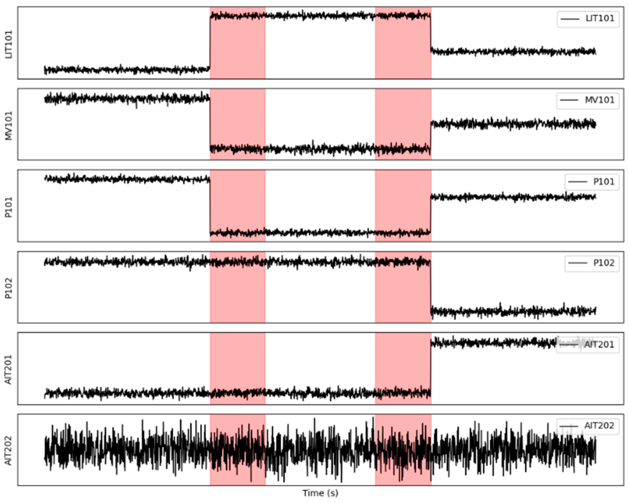
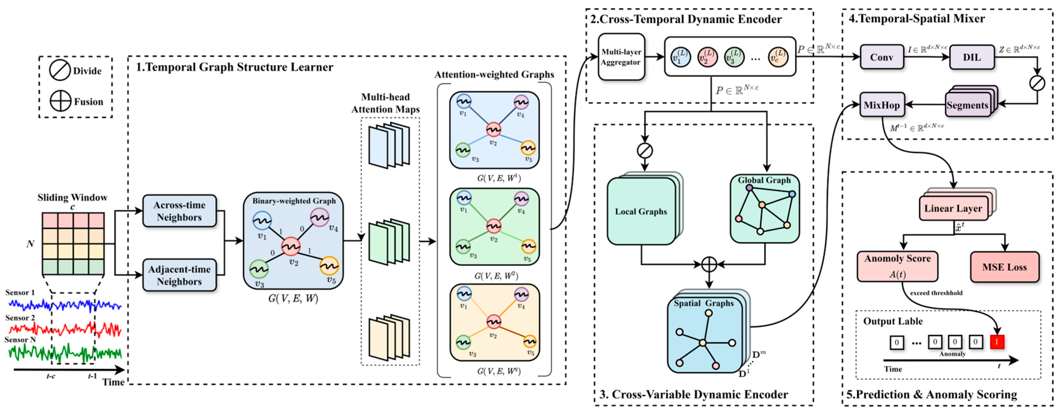
- We propose a novel deep learning architecture, called DTS-MixNet, for multivariate time series anomaly detection. It uniquely integrates dynamic graph learning across both temporal dimension and spatial (variable) one.
- Temporal Graph Structure Learner (TGSL) discovers evolving temporal dependencies by identifying across-time and adjacent-time neighbors and assigning attention-based edge weights via multi-head attention.
- The framework further includes the Cross-Temporal Dynamic Encoder (CTDE) and the Cross-Variable Dynamic Encoder (CVDE). The CTDE aggregates temporal dependencies within the sliding window to generate a proxy multivariate sequence (PMS), whereas the CVDE integrates both local and global inter-sensor dependencies to construct a spatial graph sequence (SGS).
- Spatiotemporal Mixer (TSM) is designed to effectively fuse the learned dynamic temporal features and the dynamic spatial graph structures. This enables the model to capture higher-order interaction patterns across both time and variables and lead to a more comprehensive representation for downstream tasks.
2. Related Works
2.1. Anomaly Detection
2.2. Multivariate Time Series
2.3. Graph Neural Network
3. Methodology
3.1. Problem Statement
3.2. Temporal Graph Structure Learner
- (1)
- Capture Neighbor Relationship
- (2)
- Evaluate Neighbor Degree
3.3. Cross-Temporal Dynamic Encoder
3.4. Cross-Variable Dynamic Encoder
3.5. Spatiotemporal Mixer
- (1)
- Generating Hidden Representations
- (2)
- Mixing Temporal and Spatial Information
3.6. Neural Network Prediction
| Algorithm 1: Pseudo-code of Training Phase |
| Input: Input signal: , Sliding window size: , Ground truth data at time : . Initialize model parameters end for Backpropagate loss and update model parameters using Adam optimizer. Output: Epoch loss end for Return trained model parameters |
4. Discussion
4.1. Anomaly Scoring
| Algorithm 2: Pseudo-code of Testing Phase |
| Input: Input signal: , Sliding window size: , Ground truth data at time t: . Output: Anomaly detection result . Initialize trained model parameters . The detection threshold is calibrated on a held-out validation set by sweeping candidate values and selecting the one that maximizes the F1-score. Append to end for Return |
4.2. Time Complexity Analysis
4.3. Scalability and Optimization
- Sparse/dilated temporal neighbors. In temporal modules, restrict attention to adjacent time steps plus at most across-time links (e.g., dilated offsets). This replaces dense interactions with .
- Approximate similarity for CVDE. When CVDE relies on DTW, employ a Sakoe–Chiba band or soft-DTW with a small bandwidth , optionally preceded by piecewise aggregate approximation (PAA). This changes per-pair cost from to with .
- Low-rank/linear attention. Replace quadratic attention with kernelized/low-rank variants so a layer scales as with small rank , rather than
- Group-level mixing. Cluster sensors into functional groups (via long-term correlation/MI or domain taxonomy), perform mixing at the group level (), then refine within groups.
4.4. Domain Applicability and Adaptation
- Domain priors for spatial graphs. Augment dynamically learned graphs with prior structure (e.g., clinical ontologies, market sector/industry taxonomies) via Laplacian or edge-level regularization, yielding prior-regularized dynamic graphs that respect domain knowledge while remaining adaptive.
- Shift-robust thresholding. Instead of a single fixed threshold, employ validation-based quantile calibration or conformal prediction for per-deployment calibration; update thresholds online with a small sliding validation buffer to accommodate regime changes.
- Self-supervised pretraining. Pretrain TGSL/CTDE with masked forecasting/reconstruction on large heterogeneous MTS, then fine-tune on the target domain; this preserves the architecture and improves data efficiency under limited labels.
4.5. Threshold Calibration and Adaptation
- (1)
- Rolling quantile calibration (lightweight).
- (2)
- Conformal prediction with a sliding calibration set.
4.6. Real-Time Deployment and Challenges
5. Experiments
5.1. Dataset
- SWaT is a model of a small-scale water treatment plant, simulating six stages of a real-world water treatment process, including chemical treatment, filtration, and purification. The plant is equipped with various sensors and actuators. The dataset consists of time series data from multiple sensors and actuators, capturing both non-anomalous operations and attack scenarios.
- WADI is a model of a water distribution network that simulates the water distribution process in the real world, covering multiple stages from water storage to distribution. This system is more complex than SWaT and involves larger-scale operations. The WADI dataset records sensor readings and actuator states, with the data also being time series, encompassing both non-anomalous operations and intentionally injected attack behaviors.
5.2. Baseline Methods
- LSTM-VAE (Long Short-Term Memory Variational Autoencoder) [46]: This model combines Long Short-Term Memory (LSTM) networks with a Variational Autoencoder (VAE), primarily used for anomaly detection in time series data. The model leverages LSTM’s ability to capture temporal dependencies and VAE’s capability in generating and modeling complex data distributions.
- DAGMM (Deep Autoencoding Gaussian Mixture Model) [47]: A deep learning method for anomaly detection that integrates an Autoencoder with a Gaussian Mixture Model (GMM). It is effective in detecting anomalies in high-dimensional data.
- MAD-GAN (Multivariate Anomaly Detection using Generative Adversarial Networks) [48]: A GAN-based method for anomaly detection in multivariate time series. MAD-GAN uses a generator-discriminator architecture to learn the distribution of time series data, detecting anomalies based on the discriminator’s ability to distinguish between non-anomalous and anomalous data.
- MTAD-GAT (Multivariate Time-series Anomaly Detection using Graph Attention Networks) [49]: This method uses Graph Attention Networks (GAT) for multivariate time series anomaly detection. It efficiently captures the complex dependencies between variables in time series data and detects anomalies by modeling dynamic changes over time.
- GDN (Graph Deviation Network) [12]: A multivariate time series anomaly detection method based on Graph Neural Networks (GNN). GDN builds and learns a relational graph between different variables in time series data, capturing the dependencies between them to detect anomalies. It identifies anomalies by learning deviations from non-anomalous behavior using GNNs.
- GRN (GRU-based Interpretable Multivariate Time Series Anomaly Detection Model) [50]: GRN is a deep learning model that combines GRU (Gated Recurrent Unit) and interpretability techniques, designed to handle multivariate time series data from multiple sensors in industrial control systems. The model learns the temporal dependencies within the time series to capture non-anomalous patterns and identifies anomalies by calculating the prediction error.
- ECNU-GNN (Edge Conditional Node Update Graph Neural Network) [51]: This model is a graph neural network-based model for multivariate time series anomaly detection, which captures complex temporal and relational dependencies by conditionally updating node states. The model represents time series data as a graph, where each node corresponds to a time step or sensor, and edges represent the relationships between them. By conditionally updating node states based on edge features, ECNU-GNN can more accurately learn non-anomalous behavior patterns and effectively detect anomalies in systems, making it particularly useful for anomaly detection in complex environments like sensor networks and industrial control systems.
5.3. Evaluation Metrics
5.4. Experimental Setup
- (1)
- Parameter Selection
- (2)
- Baseline Setup.
5.5. Comparative Study
5.6. Ablation Study
- w/o Temporal Attention: The multi-head attention mechanism (Equations (7) and (8)) within TGSL was removed. Instead, the aggregation in CTDE (Equation (10)) used simpler, non-learned weights (e.g., uniform weights based on the binary graph from Equation (6)).
- w/o Across-Time Neighbors: The learned across-time neighbors (, Equation (3)) were excluded from TGSL. Only the adjacent-time neighbors (, Equation (4)) were used to construct the temporal graph.
- w/o Temporal Graph Modeling: The entire TGSL and CTDE pipeline was bypassed. The raw input sequence was directly fed into subsequent modules, isolating the contribution of dynamic temporal graph learning and encoding.
- w/o Spatial Graphs: Local and global spatial graph ( and , Equations (12)–(14)) were replaced. Instead, a single, static graph (e.g., -Nearest Neighbors approach,) was used for the spatial mixing in TSM.
- w/o TSM Feature Enhancement: The initial feature enhancement steps within the TSM specifically the Convolution and the Dilated Inception Layer (DIL) were removed. Consequently, the Proxy Multivariate Sequence , after being segmented into , was directly fed into the MixHop component.
5.7. Interpretability of Model
- (1)
- Interpretability of Embedding Vectors for Sensors
- (2)
- Interpretability of Attacks
- (3)
- Practical Implications and Future Work
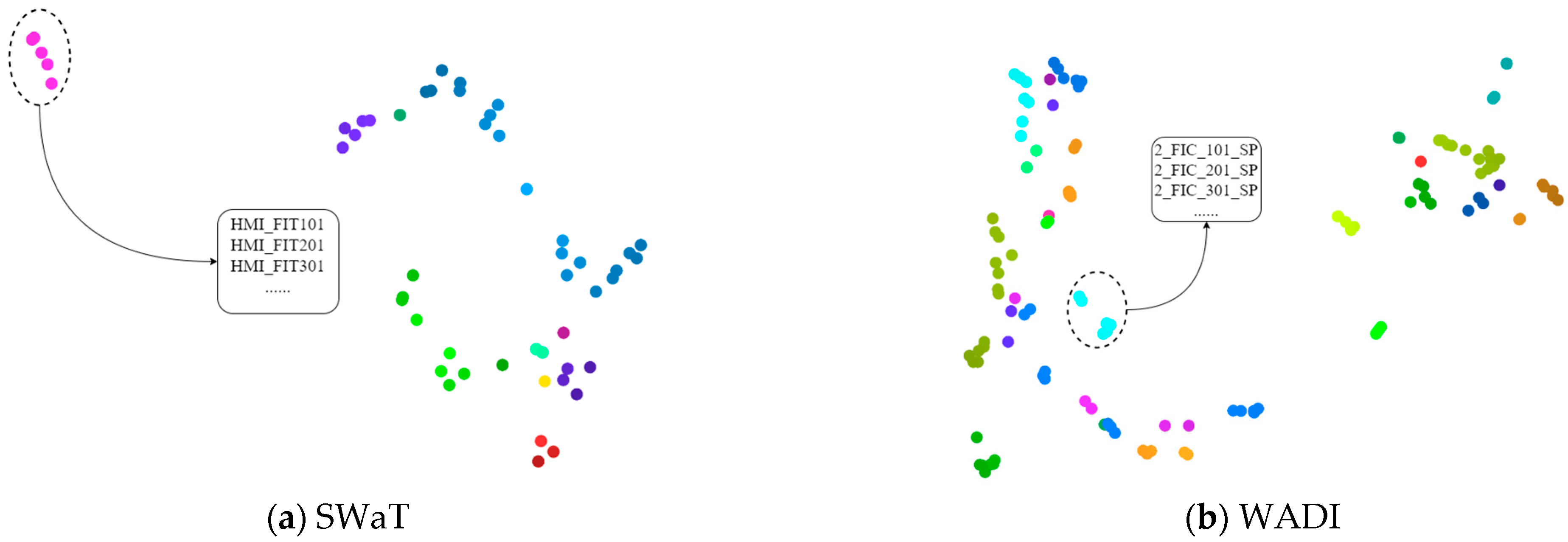
- Sensor Role Identification: By examining the clusters in the sensor embedding space, we can classify sensors based on their functional roles in the system. This could help practitioners understand which sensors are crucial for the overall system health, and prioritize them for
- Real-time Anomaly Monitoring: To improve the practical utility of our model, we are exploring ways to incorporate these interpretability features into a real-time monitoring dashboard. This would allow operators to visualize sensor embeddings, track anomalies, and identify critical sensors in the context of their system, making anomaly detection more actionable and transparent.
5.8. Correlation Heatmap Analysis
- Strong Correlations: Distinct blocks of strong positive (deep red) and negative (deep blue) correlations are clearly evident between various sensor pairs. For example, notable correlations exist within the AIT501-FIT503 sensor block. This signifies strong mutual influence or dependency between these sensors, highlighting that they cannot be effectively modeled in isolation.
- Group Structures: Clusters of sensors often exhibit similar correlation patterns when compared to other groups. For instance, the sensors in the PIT501-P603 group demonstrate cohesive behavior in their correlations. These groupings may hint at underlying functional modules or subsystems within the monitored physical process.
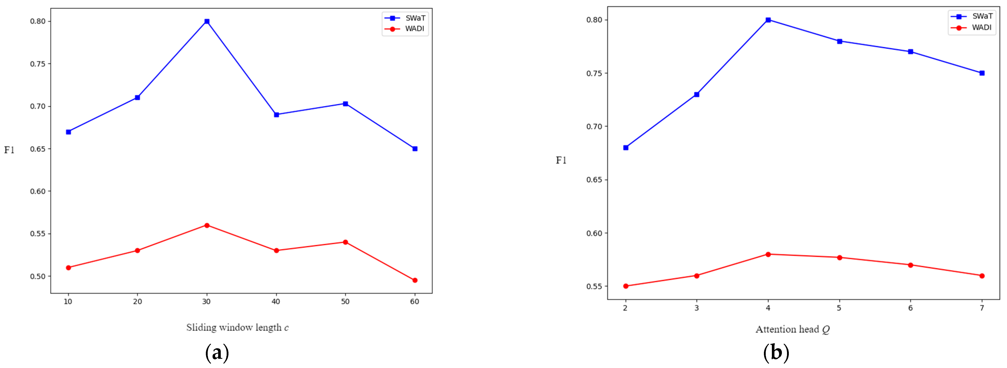
5.9. Sensitivity
- (1)
- Sliding Window Length
- (2)
- Number of Attention Heads
6. Conclusions
Author Contributions
Funding
Data Availability Statement
Conflicts of Interest
References
- Tax, D.M.J.; Duin, R.P.W. Support vector data description. Mach. Learn. 2004, 54, 45–66. [Google Scholar] [CrossRef]
- Kim, S.; Choi, Y.; Lee, M. Deep learning with support vector data description. Neurocomputing 2015, 165, 111–117. [Google Scholar] [CrossRef]
- Zhai, S.; Cheng, Y.; Lu, W.; Zhang, Z. Deep structured energy based models for anomaly detection. In Proceedings of the 33rd International Conference on Machine Learning, New York, NY, USA, 19–24 June 2016; Volume 48, pp. 1100–1109. [Google Scholar]
- Angiulli, F.; Pizzuti, C. Fast Outlier Detection in High Dimensional Spaces. In Principles of Data Mining and Knowledge Discovery; Springer: Berlin/Heidelberg, Germany, 2002; pp. 15–27. [Google Scholar]
- Keogh, E.; Lin, J.; Fu, A. HOT SAX: Efficiently finding the most unusual time series subsequence. In Proceedings of the Fifth IEEE International Conference on Data Mining (ICDM’05), Houston, TX, USA, 27–30 November 2005. [Google Scholar]
- Mathur, A.P.; Tippenhauer, N.O. SWaT: A water treatment testbed for research and training on ICS security. In Proceedings of the 2016 International Workshop on Cyber-Physical Systems for Smart Water Networks (CySWater), Vienna, Austria, 11 April 2016; pp. 31–36. [Google Scholar]
- Choi, K.; Yi, J.; Park, C.; Yoon, S. Deep learning for anomaly detection in time-series data: Review, analysis, and guidelines. IEEE Access 2021, 9, 120043–120065. [Google Scholar] [CrossRef]
- Wen, T.; Keyes, R. Time series anomaly detection using convolutional neural networks and transfer learning. arXiv 2019, arXiv:1905.13628. Available online: https://arxiv.org/abs/1905.13628 (accessed on 13 July 2025). [CrossRef]
- An, J.; Cho, S. Variational autoencoder based anomaly detection using reconstruction probability. Spec. Lect. IE 2015, 2, 1–18. [Google Scholar]
- Akcay, S.; Atapour-Abarghouei, A.; Breckon, T.P. GANomaly: Semi-supervised anomaly detection via adversarial training. In Computer Vision—ACCV 2018; Springer: Cham, Switzerland, 2019; pp. 622–637. [Google Scholar]
- Lin, S.; Clark, R.; Birke, R.; Schönborn, S.; Trigoni, N.; Roberts, S. Anomaly detection for time series using VAE-LSTM hybrid model. In Proceedings of the ICASSP 2020—2020 IEEE International Conference on Acoustics, Speech and Signal Processing (ICASSP), Barcelona, Spain, 4–8 May 2020; pp. 4322–4326. [Google Scholar]
- Deng, A.; Hooi, B. Graph neural network-based anomaly detection in multivariate time series. In Proceedings of the AAAI Conference on Artificial Intelligence, Virtual, 2–9 February 2021; Volume 35, pp. 4027–4035. [Google Scholar]
- Zhang, W.; Zhang, C.; Tsung, F. GRELEN: Multivariate time series anomaly detection from the perspective of graph relational learning. In Proceedings of the Thirty-First International Joint Conference on Artificial Intelligence, Vienna, Austria, 23–29 July 2022; pp. 2390–2397. [Google Scholar]
- Chen, K.; Feng, M.; Wirjanto, T.S. Multivariate time series anomaly detection via dynamic graph forecasting. arXiv 2023, arXiv:2302.02051. Available online: https://arxiv.org/abs/2302.02051 (accessed on 13 July 2025). [CrossRef]
- Yin, S.; Ding, S.X.; Haghani, A.; Hao, H.; Zhang, P. A comparison study of basic data-driven fault diagnosis and process monitoring methods on the benchmark Tennessee Eastman process. J. Process Control 2012, 22, 1567–1581. [Google Scholar] [CrossRef]
- MacGregor, J.F.; Jaeckle, C.; Kiparissides, C.; Koutoudi, M. Process monitoring and diagnosis by multiblock PLS methods. AIChE J. 1994, 40, 826–838. [Google Scholar] [CrossRef]
- Russell, E.L.; Chiang, L.H.; Braatz, R.D. Fault detection in industrial processes using canonical variate analysis and dynamic principal component analysis. Chemom. Intell. Lab. Syst. 2000, 51, 81–93. [Google Scholar] [CrossRef]
- Schlegl, T.; Seebock, P.; Waldstein, S.M.; Langs, G.; Schmidt-Erfurthb, U. f-AnoGAN: Fast unsupervised anomaly detection with generative adversarial networks. Med. Image Anal. 2019, 54, 30–44. [Google Scholar] [CrossRef]
- Zhou, C.; Paffenroth, R.C. Anomaly detection with robust deep autoencoders. In Proceedings of the 23rd ACM SIGKDD International Conference on Knowledge Discovery and Data Mining, Halifax, NS, Canada, 13 August 2017; pp. 665–674. [Google Scholar]
- Jang, J.; Lee, H.H.; Park, J.A.; Kim, H. Unsupervised anomaly detection using generative adversarial networks in 1H-MRS of the brain. J. Magn. Reson. 2021, 325, 106936. [Google Scholar] [CrossRef]
- Staar, B.; Lütjen, M.; Freitag, M. Anomaly detection with convolutional neural networks for industrial surface inspection. Procedia CIRP 2019, 79, 484–489. [Google Scholar] [CrossRef]
- Zivot, E.; Wang, J. Vector autoregressive models for multivariate time series. In Modeling Financial Time Series with S-PLUS®; Springer: New York, NY, USA, 2006; pp. 385–429. [Google Scholar]
- Box, G.E.; Pierce, D.A. Distribution of residual autocorrelations in autoregressive-integrated moving average time series models. J. Am. Stat. Assoc. 1970, 65, 1509–1526. [Google Scholar] [CrossRef]
- Cao, L.J.; Tay, F.E.H. Support vector machine with adaptive parameters in financial time series forecasting. IEEE Trans. Neural Netw. 2003, 14, 1506–1518. [Google Scholar] [CrossRef]
- Connor, J.T.; Martin, R.D.; Atlas, L.E. Recurrent neural networks and robust time series prediction. IEEE Trans. Neural Netw. 1994, 5, 240–254. [Google Scholar] [CrossRef]
- Zhao, B.; Lu, H.; Chen, S.; Liu, J.; Wu, D. Convolutional neural networks for time series classification. J. Syst. Eng. Electron. 2017, 28, 162–169. [Google Scholar] [CrossRef]
- Borovykh, A.; Bohte, S.; Oosterlee, C.W. Conditional time series forecasting with convolutional neural networks. arXiv 2018, arXiv:1703.04691. Available online: https://arxiv.org/abs/1703.04691 (accessed on 16 July 2025). [CrossRef]
- Wen, Q.; Zhou, T.; Zhang, C.; Chen, W.; Ma, Z.; Yan, J.; Sun, L. Transformers in time series: A survey. In Proceedings of the Thirty-Second International Joint Conference on Artificial Intelligence, IJCAI-23, Macao, China, 19–25 August 2023; pp. 6778–6786. [Google Scholar]
- Hochreiter, S.; Schmidhuber, J. Long short-term memory. Neural Comput. 1997, 9, 1735–1780. [Google Scholar] [CrossRef]
- Chung, J.; Gulcehre, C.; Cho, K.; Bengio, Y. Empirical evaluation of gated recurrent neural networks on sequence modeling. arXiv 2014, arXiv:1412.3555. [Google Scholar] [CrossRef]
- Wu, Z.; Pan, S.; Chen, F.; Long, G.; Zhang, C.; Yu, P.S. A comprehensive survey on graph neural networks. IEEE Trans. Neural Netw. Learn. Syst. 2021, 32, 4–24. [Google Scholar] [CrossRef]
- Zhang, R.; Zhou, Z.; Zuo, Y.; Cui, Y.; Zhang, Z. Multivariate time series anomaly detection based on graph neural network and grated neural network. In Proceedings of the International Conference on Cyber Security, Artificial Intelligence, and Digital Economy (CSAIDE 2023), Nanjing, China, 3–5 March 2023; Volume 12718, p. 127180R. [Google Scholar]
- Xu, K.; Li, Y.; Li, Y.; Xu, L.; Li, R.; Dong, Z. Masked graph neural networks for unsupervised anomaly detection in multivariate time series. Sensors 2023, 23, 7552. [Google Scholar] [CrossRef]
- Lee, J.; Park, B.; Chae, D.K. DuoGAT: Dual time-oriented graph attention networks for accurate, efficient and explainable anomaly detection on time-series. In Proceedings of the 32nd ACM International Conference on Information and Knowledge Management, Birmingham, UK, 21–25 October 2023; pp. 1188–1197. [Google Scholar]
- Zhou, J.; Cui, G.; Hu, S.; Zhang, Z.; Yang, C.; Liu, Z.; Wang, L.; Li, C.; Sun, M. Graph neural networks: A review of methods and applications. AI Open 2020, 1, 57–81. [Google Scholar] [CrossRef]
- Scarselli, F.; Gori, M.; Tsoi, A.C.; Hagenbuchner, M.; Monfardini, G. The graph neural network model. IEEE Trans. Neural Netw. 2009, 20, 61–80. [Google Scholar] [CrossRef]
- Bruna, J.; Zaremba, W.; Szlam, A.; LeCun, Y. Spectral networks and locally connected networks on graphs. arXiv 2013, arXiv:1312.6203. Available online: https://arxiv.org/abs/1312.6203 (accessed on 16 July 2025).
- Henaff, M.; Bruna, J.; LeCun, Y. Deep convolutional networks on graph-structured data. arXiv 2015, arXiv:1506.05163. Available online: https://arxiv.org/abs/1506.05163 (accessed on 16 July 2025). [CrossRef]
- Defferrard, M.; Bresson, X.; Vandergheynst, P. Convolutional neural networks on graphs with fast localized spectral filtering. In Advances in Neural Information Processing Systems; MIT Press: Cambridge, MA, USA, 2016; p. 29. [Google Scholar]
- Kipf, T.N.; Welling, M. Semi-supervised classification with graph convolutional networks. arXiv 2016, arXiv:1609.02907. Available online: https://arxiv.org/abs/1609.02907 (accessed on 16 July 2025).
- Velickovic, P.; Cucurull, G.; Casanova, A.; Romero, A.; Lio, P.; Bengio, Y. Graph attention networks. Stat 2017, 1050, 10–48550. [Google Scholar]
- Müller, M. Dynamic time warping. In Information Retrieval for Music and Motion; Springer: Berlin/Heidelberg, Germany, 2007; pp. 69–84. [Google Scholar]
- Wu, Z.; Pan, S.; Long, G.; Jiang, J.; Chang, X.; Zhang, C. Connecting the dots: Multivariate time series forecasting with graph neural networks. In Proceedings of the 26th ACM SIGKDD International Conference on Knowledge Discovery & Data Mining, Virtual, 6–10 July 2020; pp. 753–763. [Google Scholar]
- Abu-El-Haija, S.; Perozzi, B.; Kapoor, A.; Alipourfard, N.; Lerman, K.; Harutyunyan, H.; Steeg, G.V.; Salstyan, A. MixHop: Higher-order graph convolutional architectures via sparsified neighborhood mixing. In Proceedings of the 36th International Conference on Machine Learning, Long Beach, CA, USA, 9–15 June 2019; Volume 97, pp. 21–29. [Google Scholar]
- Ahmed, C.M.; Palleti, V.R.; Mathur, A.P. WADI: A water distribution testbed for research in the design of secure cyber physical systems. In Proceedings of the 3rd International Workshop on Cyber-Physical Systems for Smart Water Networks, Pittsburgh, PA, USA, 21 April 2017; pp. 25–28. [Google Scholar]
- Park, D.; Hoshi, Y.; Kemp, C.C. A multimodal anomaly detector for robot-assisted feeding using an LSTM-based variational autoencoder. IEEE Robot. Autom. Lett. 2018, 3, 1544–1551. [Google Scholar] [CrossRef]
- Zong, B.; Song, Q.; Min, M.R.; Cheng, W.; Lumezanu, C.; Cho, D.; Chen, H. Deep autoencoding gaussian mixture model for unsupervised anomaly detection. In Proceedings of the 6th International Conference on Learning Representations, Vancouver, BC, Canada, 30 April–3 May 2018; pp. 1–19. [Google Scholar]
- Li, D.; Chen, D.; Jin, B.; Shi, L.; Goh, J.; Ng, S.K. MAD-GAN: Multivariate anomaly detection for time series data with generative adversarial networks. In Artificial Neural Networks and Machine Learning—ICANN 2019: Text and Time Series; Springer: Cham, Switzerland, 2019; pp. 703–716. [Google Scholar]
- Zhao, H.; Wang, Y.; Duan, J.; Huang, C.; Cao, D.; Tong, Y.; Xu, B.; Bai, J.; Zhang, Q. Multivariate time-series anomaly detection via graph attention network. In Proceedings of the 2020 IEEE International Conference on Data Mining (ICDM), Sorrento, Italy, 17–20 November 2020; pp. 841–850. [Google Scholar]
- Tang, C.; Xu, L.; Yang, B.; Tang, Y.; Zhao, D. GRU-based interpretable multivariate time series anomaly detection in industrial control system. Comput. Secur. 2023, 127, 103094. [Google Scholar] [CrossRef]
- Jo, H.; Lee, S.W. Edge conditional node update graph neural network for multivariate time series anomaly detection. Inf. Sci. 2024, 679, 121062. [Google Scholar] [CrossRef]
- Maaten, L.V.D.; Hinton, G. Visualizing data using t-SNE. J. Mach. Learn. Res. 2008, 9, 2579–2605. [Google Scholar]


| Notations | Descriptions | Notations | Descriptions |
|---|---|---|---|
| Training data sampled on N sensors and T time steps | Proxy Multivariate Sequence (PMS) | ||
| Test data sampled on N sensors and U time steps | The i-th locality with w = c/m | ||
| Sensor data at time t in a sliding window of size c | The j-th row in the i-th locality | ||
| Sensor data at time t | Local spatial adjacency matrix for the i-th locality | ||
| Predicted data at time t | Global spatial adjacency matrix | ||
| Binary-weighted graph | Fused spatial adjacency matrix for the i-th locality | ||
| Attention-weighted graph under multi-head attention | Spatial Graph Sequence (SGS) | ||
| Learnable vectors for nodes | d | Number of channels | |
| Relationship matrix for measuring the time closeness | Feature representation after Conv in TSM | ||
| K | Number of nearest neighbors | Hidden representation in TSM | |
| Across-time neighbors of node | The i-th segment of hidden representation Z | ||
| Adjacent-time neighbors of node | The i-th feature matrix by mixing and | ||
| Neighbors of node | Final representation of sliding window | ||
| Learnable mapping matrix for the q-th attention head | , | Hyperparameter scaling DTW distance | |
| Learnable vector for scoring neighbors in q-th attention head | Learnable parameters |
| Module | Complexity Per Window | Description |
|---|---|---|
| TGSL | Constructing the temporal graph structure | |
| CTDE (L layers) | Encoding temporal dependencies | |
| CVDE | Encoding cross-variable dependencies | |
| TSM and Predict | Mixing temporal and spatial information | |
| Whole DTS-MixNet | Total complexity of the entire model | |
| Training Phase Total | Total complexity of the entire training | |
| Testing Phase Total | Total complexity of the entire testing |
| Datasets | # Features | # Train | # Test | Anomalies |
|---|---|---|---|---|
| SWaT | 51 | 47,520 | 44,991 | 12.22% |
| WADI | 127 | 76,297 | 17,280 | 5.84% |
| Hyperparameter | Search Range |
|---|---|
| Window length | |
| Attention heads | |
| Across-time neighbors | SWaT: ; WADI: |
| Hidden channels | |
| DTW scaling | |
| Learning rate | |
| DIL kernel set |
| SWaT | WADI | |||||
|---|---|---|---|---|---|---|
| Methods | Pre | Rec | F1 | Pre | Rec | F1 |
| LSTM-VAE [46] | 96.24 | 59.91 | 0.7384 | 84.79 | 14.45 | 0.2469 |
| DAGMM [47] | 27.46 | 69.52 | 0.3936 | 54.44 | 26.99 | 0.3608 |
| MAD-GAN [48] | 96.58 | 57.50 | 0.7206 | 87.33 | 14.87 | 0.2541 |
| MTAD-GAT [49] | 95.15 | 61.87 | 0.7495 | 62.10 | 18.57 | 0.2645 |
| GDN [12] | 88.03 | 62.75 | 0.7280 | 66.25 | 31.10 | 0.4206 |
| GRN [50] | 98.37 | 61.09 | 0.7537 | 35.84 | 73.98 | 0.4828 |
| ECNU-GNN [51] | 98.45 | 68.91 | 0.8089 | 76.52 | 46.10 | 0.5730 |
| DTS-MixNet (Ours) | 98.59 | 69.58 | 0.8158 | 87.34 | 43.65 | 0.5821 |
| Settings | SWaT | WADI |
|---|---|---|
| DTS-MixNet | 98.59 | 87.34 |
| DTS-MixNet w/o. Temporal Attention | 87.58 | 80.78 |
| DTS-MixNet w/o. Across-Time Neighbors | 93.14 | 84.34 |
| DTS-MixNet w/o. Temporal Graph Modeling | 83.29 | 72.36 |
| DTS-MixNet w/o. Spatial Graphs | 86.78 | 76.57 |
| DTS-MixNet w/o. TSM Feature Enhancement | 83.37 | 78.43 |
Disclaimer/Publisher’s Note: The statements, opinions and data contained in all publications are solely those of the individual author(s) and contributor(s) and not of MDPI and/or the editor(s). MDPI and/or the editor(s) disclaim responsibility for any injury to people or property resulting from any ideas, methods, instructions or products referred to in the content. |
© 2025 by the authors. Licensee MDPI, Basel, Switzerland. This article is an open access article distributed under the terms and conditions of the Creative Commons Attribution (CC BY) license (https://creativecommons.org/licenses/by/4.0/).
Share and Cite
Tan, C.; Hu, J.; Li, J.; Miao, M.; Hu, W.; Wang, S. DTS-MixNet: Dynamic Spatiotemporal Graph Mixed Network for Anomaly Detection in Multivariate Time Series. Big Data Cogn. Comput. 2025, 9, 245. https://doi.org/10.3390/bdcc9100245
Tan C, Hu J, Li J, Miao M, Hu W, Wang S. DTS-MixNet: Dynamic Spatiotemporal Graph Mixed Network for Anomaly Detection in Multivariate Time Series. Big Data and Cognitive Computing. 2025; 9(10):245. https://doi.org/10.3390/bdcc9100245
Chicago/Turabian StyleTan, Chengxun, Jiayi Hu, Jian Li, Minmin Miao, Wenjun Hu, and Shitong Wang. 2025. "DTS-MixNet: Dynamic Spatiotemporal Graph Mixed Network for Anomaly Detection in Multivariate Time Series" Big Data and Cognitive Computing 9, no. 10: 245. https://doi.org/10.3390/bdcc9100245
APA StyleTan, C., Hu, J., Li, J., Miao, M., Hu, W., & Wang, S. (2025). DTS-MixNet: Dynamic Spatiotemporal Graph Mixed Network for Anomaly Detection in Multivariate Time Series. Big Data and Cognitive Computing, 9(10), 245. https://doi.org/10.3390/bdcc9100245


