Efficient Data Augmentation Methods for Crop Disease Recognition in Sustainable Environmental Systems

Abstract

Crop diseases significantly threaten agricultural productivity, leading to unstable food supply and economic losses. The current approaches to automated crop disease recognition face challenges such as limited datasets, restricted coverage of disease types, and inefficient feature extraction, which hinder their generalization across diverse crops and disease patterns. To address these challenges, we propose an efficient data augmentation method to enhance the performance of deep learning models for crop disease recognition. By constructing a new large-scale dataset comprising 24 different classes, including both fruit and leaf samples, we intend to handle a variety of disease patterns and improve model generalization capabilities. Geometric transformations and color space augmentation techniques are applied to validate the efficiency of deep learning models, specifically convolution and transformer models, in recognizing multiple crop diseases. The experimental results show that these augmentation techniques improve classification accuracy, achieving F1 scores exceeding 98%. Feature map analysis further confirms that the models effectively capture key disease characteristics. This study underscores the importance of data augmentation in developing automated, energy-efficient, and environmentally sustainable crop disease detection solutions, contributing to more sustainable agricultural practices.

1. Introduction

Sustainable agricultural ecosystems that promote economic growth and environmental protection require a paradigm shift toward green-technology-based approaches. In this regard, the integration of ICT with AI plays a pivotal role in advancing sustainable green growth within agricultural systems [1,2]. Specifically, AI-driven methods for crop pest and disease detection can automate pest management in agricultural ecosystems and significantly reduce the usage of chemical pesticides, thus preventing environmental pollution and enhancing resource efficiency. According to the 21st Century Guidebook to Fungi [3], approximately 16% of global crops are afflicted by pests and diseases, with most agricultural areas currently relying on pesticides for pest control. Moreover, a study published in Nature Geoscience [4] reported that the 92 chemical substances found in pesticides used across 168 countries have contaminated 64% of the agricultural land. Notably, the countries with the largest shares of contaminated land are those considered the breadbaskets of Asia, which are responsible for a substantial portion of the world’s food supply.

It is crucial to reduce the use of traditional pesticides and apply machine learning technologies capable of automatically recognizing and analyzing pest patterns to resolve these issues. Machine learning, particularly deep learning, is an example of radical digital innovation in that it enables a shift from the fixed generation patterns of power plants, originally designed to supply base load power, to more flexible generation patterns [5]. With the increase in computing resources, research on pest and disease recognition using deep learning is being actively conducted [6]. Deep learning models automatically extract features from images during the training process, thus achieving high performance, necessitating large datasets. However, most current research has involved small datasets and been limited to a few types of crops infected by pests. Moreover, rather than effectively extracting various pest features, the focus has predominantly been on creating models capable of classifying three to five diseases in the same crop species. Particularly in Asia, crops affected by pests display a range of symptoms such as browning, spotting, and fine-thread formations; yet, research accurately identifying and recognizing these characteristics remains inadequate. While deep learning models optimized for maximum performance can achieve high accuracy for up to 10 types of diseases, they struggle to maintain this performance for a more extensive array of disease types [7].

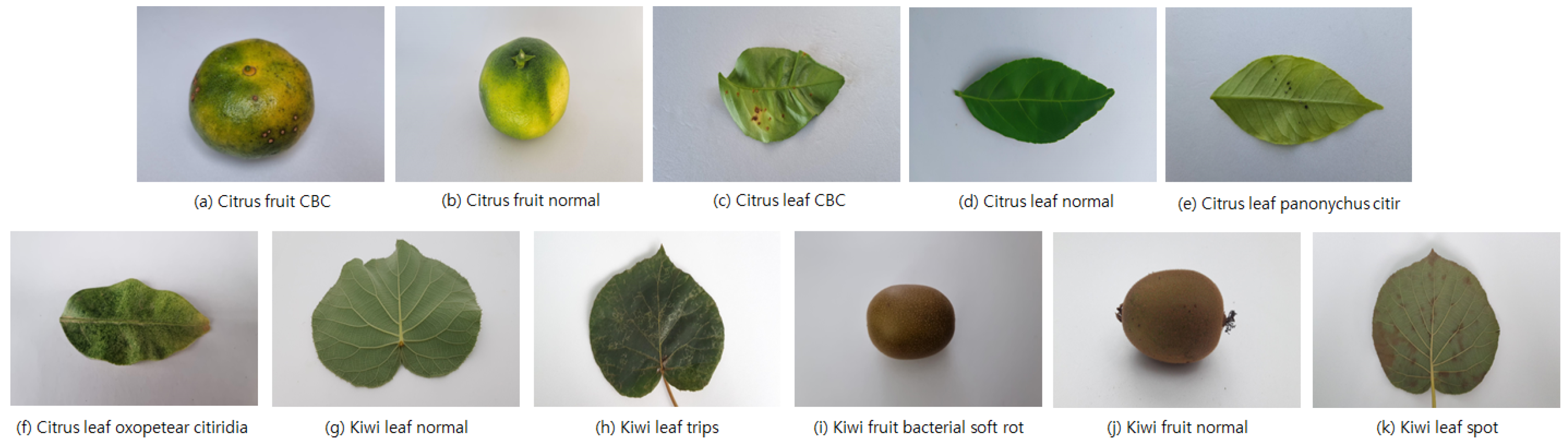
In this paper, we propose a data augmentation method that enables deep learning models to effectively extract patterns of pests and diseases, thereby addressing these issues and enabling the development of sustainable green technologies. We compared and evaluated six different deep learning models, including convolution and transformer models, for the recognition of 24 diseases across five distinct crops, creating a comprehensive pest and disease classification model. The data used in these models were augmented with over 60,000 new images, combining publicly available data from PlantVillage [8] with data on citrus and kiwi varieties collected in Asia. Our comprehensive pest and disease classification model was utilized in meticulous experiments with data augmentation techniques, subdivided into detailed categories of geometric transformations and color space transformations. The results demonstrate that considering the color distribution is crucial as the diversity in data patterns increases, as evidenced by the experimental outcomes and feature maps.

The contributions of this work are threefold:

• We collected private data on citrus and kiwi varieties and enhanced the validity of our experimental results by including the PlantVillage dataset, a public dataset. The constructed dataset comprises a total of 60,165 images, representing a large-scale dataset; however, the classes are imbalanced. We addressed the data bias problem by employing stratified cross-validation for verification.
• The data used in the experiments included 24 diseases across five types of crops. Some of these diseases are common to different crops or are the same disease affecting multiple crops. We developed a data augmentation method combining geometric and color space transformations designed to enable models to efficiently extract data patterns even for diseases across different domains.
• To validate the performance of the data augmentation methods, we compared and evaluated six deep learning models, including convolution-based and transformer-based models. The experimental results confirmed the prominence of the disease patterns in the data through feature maps, emphasizing the importance of color distribution.

The remainder of this paper is organized as follows: Section 2 provides a brief review of the related works. Section 3 discusses the data acquisition methods, preprocessing steps, and data augmentation techniques used in this study. Section 4 introduces the proposed network architecture for crop disease classification, while Section 5 presents the corresponding experimental results. In the final two sections, we present the visualizations of the feature maps based on the experimental results and discuss potential future research directions.

2. Related Work

With the exponential development of computer technology, machine learning and deep learning have been widely applied across various research fields. In particular, the agricultural sector has integrated these technologies to promote digital ecology and sustainable green practices through crop disease diagnosis [9]. While machine learning models based on user-defined features allow for shorter training times, they face challenges in handling low-quality images or ambiguous disease characteristics. In contrast, deep learning models automatically extract features, offering superior classification performance by directly analyzing data [10]. Recent advancements in lightweight models and GPU technology have significantly reduced the processing times of deep learning models, positioning them as a promising solution in sustainable agriculture [11]. As a result, deep learning is emerging as a key approach for advancing digital ecology and fostering sustainable green technology in modern agriculture.

2.1. A Study on Crop Disease Diagnosis Based on ML

Machine learning refers to algorithms that allow computer programs to automatically learn rules from data without requiring explicit programming. Machine learning techniques, as listed in

Table 1. Studies on ML-based crop disease classification methods.

Dataset	Total Images	Method	Accuracy	Reference
Corps	500	Support Vector Machines (SVMs)	90%	[12]
Pepper bacterial spot	997	K-Nearest Neighbor (KNN)	80.5%	[13]
Pepper healthy	360	Naïve Bayes (NB)	89.83%
Potato early blight	1000	Decision Tree (DT)	79.5%
Potato late blight	1000	K-Nearest Neighbor (KNN)	71%
Potato healthy	152	Artificial Neural Networks (ANNs)	51.61%

, have been adopted in agriculture to automatically classify and detect crop diseases. Santosh et al. [12] used Support Vector Machines (SVMs) to classify crop pests and diseases, achieving over 90% accuracy with 500 crop images. Appalanaidu et al. [13] analyzed the automatic classification of crop diseases using various machine learning algorithms, including Naïve Bayes (NB), Decision Tree (DT), Artificial Neural Networks (ANNs), K-Nearest Neighbor (KNN), and SVM, on the PlantVillage dataset. Their experimental results demonstrated an average accuracy of 84.31% for bell pepper and 59.83% for potato. Research on machine-learning-based crop disease recognition has achieved high performance in cases where images have clear features, as this approach requires the extraction and selection of specific characteristics from the data. In contrast, when images lack prominent features, it is not possible to expect high performance. This is a representative example of why the model did not achieve optimal performance with the PlantVillage dataset used in this study. Crop diseases can appear in different patterns, such as dot-like formations, clusters of pests, or twisted threads, depending on the type of crop and specific type of pest or disease. Therefore, given the limitations of machine-learning-based crop disease recognition research, it is necessary to pursue deep-learning-based methods that automatically extract patterns from images and learn from them [14].

2.2. A Study on Crop Disease Diagnosis Based on DL

Deep-learning-based research on crop disease recognition, a subset of machine learning, has been reported to be effective, as listed in

Table 2. Studies on DL-based crop disease classification methods.

Dataset	Total Images	Method	Accuracy	Reference
Apple	2086	VGGNet-16	90.4%	[15]
		Inception-v3	83.0%
Paddy Doctor	16,225	ResNet-34	97.50%	[16]
		MobileNet	92.42%
Maize Disease	9279	EfficientNet-b0 Transfer Learning	98.52%	[17]
Potato Late Blight	1000	DenseNet	97.8%	[18]
Potato Early Blight	1000		97.6%
Potato Leaf Roll	750		96.8%

. Deep learning involves the sequential passage of data through the layers of a neural network, which automatically extracts features from images based on the decisions made at each layer. This ability to learn from deep networks allows deep learning to achieve higher performance than traditional machine learning methods. Recent studies have focused on various aspects, including image resizing, normalization, standardization, deep learning frameworks, and optimization algorithms. Dhaka et al. [15] classified diseases in apples using the PlantVillage dataset. The experimental results demonstrated that the multilayer CNN models achieved accuracies of 90.4% for VGG16, 83% with Inception-v3 and 80.0% with ResNet50. Verma et al. [16] introduced the Paddy Doctor dataset with 16,225 annotated paddy leaf images across 13 classes to enable automated disease identification, achieving the highest accuracy of 97.50% using ResNet-34, addressing challenges in paddy disease detection. Liu et al. [17] recognized maize leaf diseases using a fine-tuned EfficientNet model based on transfer learning, achieving a maximum accuracy of 98.52% and outperforming VGG-16, Inception-v3, and ResNet-50 in both training speed and recognition performance. Mahum et al. [18] proposed an improved Efficient DenseNet model for detecting and classifying five potato leaf classes, achieving 97.2% accuracy, addressing imbalanced data challenges and outperforming existing models.

Many previous studies on crop disease diagnosis have utilized various machine learning and deep learning models but have primarily focused on detecting diseases on the leaves and addressing disease recognition in single crops. However, pests and diseases can affect multiple organs of crops, necessitating datasets that include both leaves and fruits. To achieve this, it is essential to build datasets that account for various crop types and domains while considering the specific background elements of each crop. Although high performance is typically obtained for the disease classification of single crops due to their shared domain, developing multiple models for individual diseases significantly increases energy consumption and carbon emissions. Therefore, developing a single model that can achieve high performance is crucial. To address these issues, this study expanded the PlantVillage dataset, originally containing only leaves, by incorporating citrus and kiwi varieties with both leaves and fruits, resulting in a new large dataset consisting of 24 new classes. Additionally, to assess the capability of a single model in efficiently processing a large dataset, this study employed deep learning models such as VGGNet [19], ResNet [20], DenseNet [21], EfficientNet [22], ViT [23], and DeiT [24] to conduct an experimental analysis on the effectiveness of data augmentation.

3. Data Augmentation Methods for Crop Disease Recognition

3.1. Image Acquisition

In this research, we constructed a dataset for experimental use by integrating a public dataset with private data collected from farmlands. The public dataset PlantVillage consists of crops such as potatoes, bell peppers, and tomatoes. This dataset comprises over 40,000 images of leaves. We also collected a new dataset from citrus and kiwi crops. The images were obtained from farms located in Jeju City [25], South Korea (${126}^{\circ }{08}^{\prime }{43}^{″}$∼${126}^{\circ }{58}^{\prime }{20}^{″}$ E, ${33}^{\circ }{11}^{\prime }{27}^{″}$∼${33}^{\circ }{33}^{\prime }{50}^{″}$ N). Figure 1 displays the geographic map of the study area, indicating the locations of the citrus and kiwi farms with red and blue pinpoints, respectively. All the collected images were in-field images captured directly by agricultural experts on the farms. To maintain consistent image quality, the experts adjusted the shooting height, angle, and lighting distance according to the disease types of each crop and carefully avoided shadows and light reflections during the capturing process.

The data collected were confined to the year 2021, thereby limiting the available dataset. The stages of fruit development encompass nine phases: eye formation, leaf development, branch elongation, pre-flowering, flowering, fruit enlargement, fruit ripening, senescence, and dormancy. Data were obtained from the fruit growth and ripening stages, where disease incidence is most pronounced. The data collected during the fruit growth phase, from June to October, represent 60% of the total dataset, comprising 12,000 images. During the fruit ripening phase, from November to December, an additional 8000 images were collected, accounting for 40% of the total dataset. The dataset from the ripening stage underwent two rounds of expert validation and was exclusively utilized for the test dataset. Figure 2 illustrates representative image samples from the acquired dataset.

3.2. Crop Disease Images and Dataset

To enhance the reproducibility and credibility of our study, we did not rely exclusively on the data we collected; we also incorporated the publicly available PlantVillage dataset. Information regarding the constructed dataset is presented in

Table 3. Crop disease dataset details before data cleaning. Bold denotes classes containing fewer than 1000 images.

Crop Name	Disease Name	Number of Images
Citrus	citrus fruit healthy	2545
	citrus fruit CBC	1716
	citrus leaf healthy	2455
	citrus leaf CBC	9552
	citrus leaf Panonychus citri	1814
	citrus leaf Toxoptera citricida	1918
Kiwi	kiwi fruit healthy	2124
	kiwi fruit bacterial soft rot	1737
	kiwi leaf healthy	2876
	kiwi leaf Thysanoptera	5585
	kiwi leaf spot	7678
bell pepper	bell pepper bacteria spot	997
	bell pepper healthy	1478
Potato	potato early blight	1000
	potato late blight	1000
	potato healthy	152
Tomato	tomato target spot	1404
	tomato early blight	1000
	tomato late blight	1909
	tomato leaf mold	952
	tomato septoria leaf spot	1771
	tomato spider mites	1676
	tomato mosaic virus	373
	tomato yellow leaf virus	3209
	tomato healthy	1591
	tomato bacterial spot	2127

. As shown in Table 3, the PlantVillage dataset consists of 15 classes. Among these 15 classes, there is a severe data imbalance, as the ’potato healthy’ and ’tomato mosaic virus’ classes have fewer than 500 data samples each. To address this imbalance, these two classes were excluded from this study. Subsequently, the original dataset described in Table 3 was randomly partitioned into training and test datasets in a 70:30 ratio. The test dataset was verified to contain at least 200 images after partitioning. There were a total of 5 classes in these 200 images, namely, ‘bell pepper bacteria spot’, ‘potato early blight’, ‘potato late blight’, ‘tomato leaf mold’, and ‘tomato early blight’. Following the exclusion of these 5 classes, 7 classes, including ’potato healthy’ and ’tomato mosaic virus’, were excluded due to insufficient sample size. In this study, each test dataset class was required to contain a minimum of 200 images to classify more than ten diseases. Additionally, to address the data imbalance, it was ensured that each disease class contained a minimum of 1000 images. Therefore, new images were added to the ‘bell pepper bacteria spot’ and ‘tomato leaf mold’ classes, with fewer than 800 images in the training dataset.

3.3. Generation of Insufficient Dataset

The training dataset for the ‘bell pepper bacteria spot’ class consisted of 797 images, whereas the ‘tomato leaf mold’ class consisted of 752 images. As a result, additional images were generated and incorporated into the dataset. In this study, we employed a data augmentation strategy by generating new images through the application of realistic noise to the existing dataset. Common types of noise that occur in real-world scenarios include impulse noise [26], Gaussian noise [27], multiplicative Gaussian noise [28], Poisson noise [29], uniform noise [30], and Laplacian noise [31]. Figure 3 presents representative samples of the training images with six different types of applied noise.

As shown in Figure 3, of the six types of noise, (b) and (e) exhibited significant noise levels. These two noise types pose a risk of misclassification by deep learning models and were, therefore, unsuitable for this study. Noise type (c) was excluded from the final selection due to the use of Gaussian blur [32] during the data preprocessing stage to remove noise from the field images. In contrast, (d), (f), and (g) are applicable to crop disease images. Noise type (g) affects edge intensity detection in an image, while type (f) uniformly distributes noise across the entire image. Noise type (d) applies random noise to an image and has the advantage of averaging signals collected from various positions within the wavelength range, thereby improving object detection. This method has been applied in biology and agriculture [33]. The ‘bell pepper bacteria spot’ and ‘tomato leaf mold’ classes were processed with noise type (d) to generate new images, resulting in the final dataset. The number of generated images was 3 for the ‘bell pepper bacteria spot’ disease and 48 for the ‘tomato leaf mold’ disease. The black box in Figure 3 shows the sample images generated by applying noise type (d). After data refinement, the final dataset consisted of 24 crop classes and 60,165 images. The numbers of data samples corresponding to each class are listed in

Table 4. Crop disease dataset details after data cleaning.

Disease Name	Training	Test	Total
citrus fruit healthy	2035	510	2545
citrus fruit CBC	1372	344	1716
citrus leaf healthy	1965	490	2455
citrus leaf CBC	7642	1910	9552
citrus leaf Panonychus citri	1452	362	1814
citrus leaf Toxoptera citricida	1534	384	1918
kiwi fruit healthy	1698	426	2124
kiwi fruit bacterial soft rot	1389	348	1737
kiwi leaf healthy	2300	576	2876
kiwi leaf Thysanoptera	4467	1118	5585
kiwi leaf spot	6142	1536	7678
bell pepper bacteria spot	800	200	1000
bell pepper healthy	1182	296	1478
potato early blight	800	200	1000
potato late blight	800	200	1000
tomato target spot	1095	309	1404
tomato early blight	800	200	1000
tomato late blight	1555	354	1909
tomato leaf mold	800	200	1000
tomato septoria leaf spot	1432	339	1771
tomato spider mites	1319	357	1676
tomato yellow leaf virus	2578	631	3209
tomato healthy	1269	322	1591
tomato bacterial spot	1687	440	2127

.

3.4. Data Augmentation Methods for Crop Disease Recognition

Data augmentation methods address the fundamental issue of insufficient datasets in deep learning without modifying the model structure. This straightforward technique can enhance model performance through fundamental operations. In the agricultural domain, where collecting disease data is challenging, data augmentation methods are frequently employed during data preprocessing. Choosing an appropriate data augmentation method is crucial due to the complex and diverse patterns of diseases caused by pests and pathogens in agriculture. However, existing research has focused more on optimizing models rather than investigating preprocessing approaches that enable deep learning models to better learn the characteristics of pests and crop diseases. These methods encounter limitations as the number of disease types in crops increases, making it challenging to improve model performance. Therefore, there is a need for research on data augmentation fusion approaches that effectively extract disease patterns from images while preserving important objects and avoiding excessive mixing of augmentation techniques.

There are two main categories of data augmentation methods: geometric transformations and color space transformations. Geometric transformations include horizontal and vertical flipping, rotation, resized cropping and flipping, affine transformations, and perspective transformations. Figure 4 shows sample images from all classes in the dataset created for this study. Affine and perspective transformations modify the spatial configuration of the images. These two techniques introduce the risk of image distortion as they further transform the spatial perspective of images that are already viewed from various angles. Therefore, we utilized only the geometric transformations of horizontal and vertical flipping, rotation, and resized cropping and flipping, excluding affine and perspective transformations.

Color space transformation is a data augmentation method that alters the colors of the original image. Data augmentation methods that only modify the geometric structure of the image without introducing color variations can lead to reduced representation quality, as the network focuses on identifying color combinations rather than the intrinsic visual features of the original image. Therefore, in this study, the applicability of color space transformations to the constructed crop disease images was evaluated to determine their effectiveness.

Similar to other techniques, color inversion and grayscale transformations are intended to highlight the patterns of diseases found in the image. However, they may not be suitable for cases in which the contrast levels of colors, as indicated by the red box in Figure 4, do not display substantial differences. In contrast, the color jitter augmentation method allows users to adjust the brightness, contrast, saturation, and hue of the image, thereby enabling controlled color distortions within a range that avoids blurring disease-related objects. Particularly, brightness and contrast adjustments can mimic the different environmental conditions found in actual agricultural settings. For example, reducing the brightness can simulate images captured in darker environments, whereas increasing the brightness can simulate images captured in well-lit areas during daylight hours. Therefore, this study conducted experiments by gradually increasing the intensity from 0% to 50%. As a result, randomly applying brightness, contrast, and saturation within a range of up to 35% resulted in optimal performance. Additionally, to preserve the original colors of the images and avoid abrupt color transitions that could lead to the loss of disease features, hue intensity was modified within a range of up to 10%. Sample images with these intensity adjustments are shown in Figure 5.

The citrus and kiwi datasets had comparatively clean and high-resolution images compared to the other datasets. In addition, disease images in the citrus and kiwi datasets were captured indoors, where indoor lighting was more prominent than sunlight. However, the potato, bell pepper, and tomato datasets were captured under sunlight, which resulted in noticeable shadows in the images. The blue boxes highlight images with solid shadows in Figure 4. Therefore, in this study, Gaussian blur using a kernel filter was applied to remove the noise caused by indoor lighting and sunlight. Upon examining all plant disease images of the citrus, kiwi, bell pepper, potato, and tomato crops, the final selected data augmentation methods were horizontal flipping, vertical flipping, rotation, resizing and cropping, Gaussian blur, and color jitter. Combining all six data augmentation methods could lead to a loss of patterns in leaf texture and veins. Therefore, this study selected four data augmentation methods for combination. The selection criteria were as follows: strategy (a) employs all geometric transformation techniques, whereas strategy (b) reduces the reliance on geometric transformations and focuses on employing color jitter and Gaussian blur. Strategies (a) and (b) are illustrated in the network architecture depicted in Figure 6.

4. Network Architecture

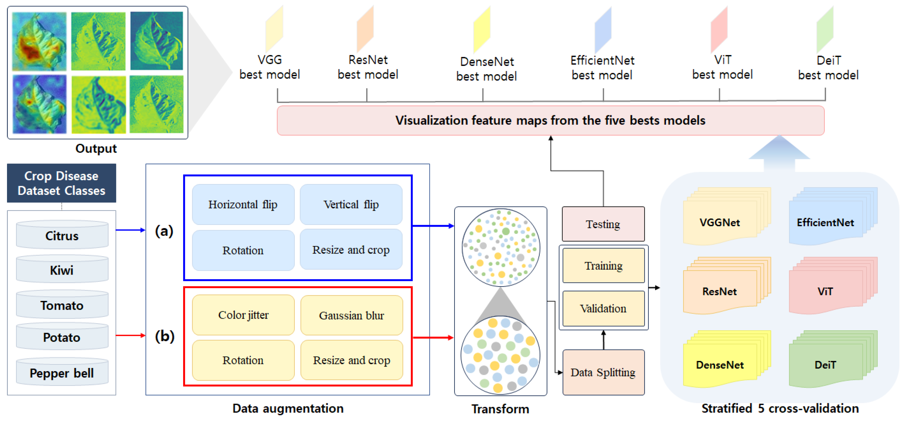
This section describes the network architecture for crop disease recognition proposed in this paper. This network architecture saves the weights of the model that yield the highest performance and uses them for model testing and feature map visualization. The network architecture is depicted in Figure 6. It is divided into three main sections: data transformation, model training, and model testing with feature map visualization. During the data transformation process, it is essential to standardize the sizes of the images originating from different sources. The images in the public dataset are formatted at $224\times 224$ pixels, while those in the private dataset are $1920\times 1920$ pixels in size. Therefore, after resizing the input images to $224\times 224$, we conducted experiments by dividing the data augmentation methods into strategy (a) and strategy (b) based on the disease patterns in the images. The methods employed for data augmentation included noise removal, color transformations, and geometric transformations. The criteria for selecting strategies (a) and (b) are explained in detail in Section 3.

In the model training stage, the network was trained using the VGGNet, ResNet, DenseNet, EfficientNet, ViT, and DeiT models pretrained on the ImageNet dataset. As the pretrained models had 1000 output nodes, this study modified the model architecture by removing the existing output layer of each pretrained model and replacing it with 24 new output layers to match the constructed dataset. Furthermore, the model training followed a fine-tuning approach in which the pretrained model’s architectures were utilized and trained with the new dataset. Training and validation were conducted using stratified k-fold cross-validation, considering the data distribution.  Stratified k-fold cross-validation helped alleviate the dataset imbalance issue. The weights of the model that achieved the highest F1 score during the training process were validated using the test dataset and utilized to extract feature maps. The experimental results of the network structure are explained in Section 5. The workflow of the network architecture is summarized in Algorithm 1.

Algorithm 1 Network architecture.

Input: Crop Classification Data ⁡  x = input_data()  x = data_augmentation(x) ⁡  k_fold = initialize_k_fold()  epochs = initialize_epochs() ⁡  for fold in $k\_fold$ do      train_data = stratified_xth_fold_train_data(x, fold)      validation_data = stratified_xth_fold_validation_data(x, fold)      models = load_model()      for model in models do          max_f1_score = 0          for epoch in $epochs$ do             train_model(model, train_data)             f1_score = validate_model(model, validation_data)             if max_f1_score < f1_score then                 max_f1_score = f1_score             end if          end for      end for      save_states(model)      show_feature_map(model)  end for

VGGNet [19], proposed by the Oxford University research team, highlights the critical role of network depth in improving CNN performance. By significantly deepening the architecture, VGGNet reduced the error rate from 16.4% to 7.3% in the ImageNet Large Scale Visual Recognition Challenge (ILSVRC) [34]. A key innovation of VGGNet is the consistent use of a $3\times 3$ filter size across all convolutional layers, optimizing computational efficiency and reducing the parameter space, enabling deeper and more expressive architectures. VGGNet16 consists of 13 convolutional layers and 3 fully connected layers, utilizing ReLU activation to accelerate training by addressing saturation issues. Dropout mitigates overfitting, and the final softmax layer outputs a probability distribution. These features showcase VGGNet’s ability to capture hierarchical representations while maintaining computational efficiency.

ResNet [20] addresses the gradient vanishing and exploding problems in deep neural networks by introducing the residual block, which leverages skip connections to directly incorporate the input x into the output. This reformulates the optimization objective to minimize the residual function $F\left(x\right)=H\left(x\right)-x$, preserving stable gradient flow during backpropagation and mitigating the vanishing gradient problem. Unlike plain architectures such as CNN, AlexNet [35], and VGGNet, which degrade as depth increases, ResNet enables the construction of much deeper networks, reaching up to 152 layers, without performance loss due to its residual learning paradigm. Additionally, ResNet employs a bottleneck design with $1\times 1$ convolutional layers to enhance computational efficiency while maintaining strong representational capacity. These innovations allow ResNet to surpass models like VGGNet and GoogleNet [36] in both efficiency and predictive performance, verifying its impact on deep learning architecture design.

DenseNet [21] is a neural network architecture that connects all layers directly via concatenation, enabling each layer to access the feature maps of all preceding layers. This design achieves superior performance with fewer parameters than ResNet. Unlike ResNet, which uses skip connections through element-wise addition, DenseNet employs concatenation, progressively increasing feature channels as layers are added. To manage this growth, DenseNet reduces the number of channels per layer and standardizes feature map dimensions for efficient concatenation. The architecture uses dense blocks to facilitate feature reuse and pooling operations. Bottleneck layers further enhance efficiency by limiting inputs to the $3\times 3$ convolutional layers to $4k$, where each layer generates k feature maps. DenseNet supports 121-, 169-, 201-, and 264-layer configurations, providing deeper networks with greater parameter efficiency than ResNet.

EfficientNet [22] is a state-of-the-art architecture for image classification that optimizes the balance between network depth, width, and input resolution to improve performance. Traditional models like VGGNet, GoogleNet, ResNet, and DenseNet primarily focus on increasing depth, with manual adjustments to width and resolution based on computational constraints. This heuristic approach often overlooks the interdependence of these dimensions. EfficientNet addresses this limitation by introducing a compound scaling method that systematically balances depth, width, and resolution, preventing the performance saturation observed in independent scaling. By using constants determined through grid search and user-defined computation budgets, EfficientNet scales performance proportionally to resources. This design allows EfficientNet to extract salient image features efficiently, maintaining parameter efficiency and enabling faster inference compared to earlier architectures.

ViT [23] is a paradigm-shifting model that extends the transformer architecture, originally developed for natural language processing, to computer vision tasks. Departing from traditional CNN-based architectures, ViT employs transformers to overcome the limitations of conventional attention mechanisms, achieving state-of-the-art performance with modest computational overhead. The training pipeline involves segmenting an image into fixed-size patches, which are linearly embedded with positional encodings and fed into the transformer encoder. Since transformers operate on 1D sequences, the flattened patches are projected into a sequential representation suitable for processing. The transformer encoder’s output is passed through a multilayer perceptron (MLP) head for image classification. ViT demonstrates exceptional computational efficiency and scalability, achieving superior performance on large-scale datasets without degradation or saturation, and can handle up to 100 billion parameters. However, its reliance on extensive pretraining with large datasets remains a significant constraint.

DeiT [24] is a model proposed by Facebook AI that enhances the efficiency of ViT by significantly reducing data and computational requirements while achieving comparable accuracy. In contrast to ViT, which necessitates pretraining on extensive datasets like JFT-300M, DeiT attains state-of-the-art performance using only the ImageNet dataset, with training completed in three days on a single 8 GPU setup. DeiT leverages hard-label knowledge distillation, transferring informative representations from a CNN teacher model to imbue the transformer with inductive bias, thereby improving generalization and performance. In hard-label distillation, the model minimizes the cross-entropy loss as

$${\mathcal{L}}_{\mathrm{distillation}}=-\sum _{i=1}^N{y}_{i}log{\widehat{y}}_i$$

(1)

where $y_i$ represents the label predicted by the teacher model, and ${\widehat{y}}_i$ is the predicted probability of the student model for class i. This approach avoids the use of temperature scaling and additional hyperparameters, making it computationally efficient. Furthermore, DeiT incorporates a distillation token, [DIST], analogous to the class token in ViT, which interacts with other embeddings via self-attention. The output of the distillation token is jointly optimized with the ground truth labels through the combined loss function:

$${\mathcal{L}}_{\mathrm{total}}=\alpha {\mathcal{L}}_{\mathrm{distillation}}+(1-\alpha ){\mathcal{L}}_{\mathrm{ground}\mathrm{truth}}$$

(2)

where $\alpha$ balances the contributions of the distillation and ground truth losses. This methodology establishes DeiT as a computationally efficient and data-effective transformer-based architecture for image classification tasks, overcoming the heavy reliance on large-scale datasets and high-specification hardware required by ViT.

5. Experiments

In this section, we present empirical evidence regarding the performance of the crop disease recognition network, which is based on the combination of data augmentation methods proposed in this study. Specifically, we report the experimental results, and we analyzed the feature maps of the proposed model. The experiments in this study were conducted on a PC with an Intel^® Core^™ i9-9900KF CPU @ 3.60 GHz, NVIDIA TITAN RTX, and Windows 10, using the Python 3.8 environment to validate the performance of the DeiT model. The remaining models were evaluated on a PC with an Intel^® Xeon^® Silver 4208 CPU @ 2.10 GHz, NVIDIA TESLA V100 32 GB, and Ubuntu 18.04.6 LTS, using the Python 3.10 environment to assess the performance of the proposed network.

5.1. Experimental Settings

The crop disease classification model utilized six pretrained deep learning models: VGGNet, ResNet, DenseNet, EfficientNet, ViT, and DeiT. The input sizes of the models varied depending on their size and type. To examine the performance differences of the combined data augmentation methods in the same environment, the input size for all six models was standardized to $224\times 224$. The images, resized to $224\times 224$ pixels as described in Section 5, underwent data preprocessing based on strategies (a) and (b). The test dataset, which was used for model validation, underwent only resizing, tensor conversion, and normalization without data augmentation for image transformation.

The training and validation datasets were divided into five folds per class for cross-validation, with the model trained on the corresponding fold for each class. The crop pest and disease classification model was trained and validated for 100 epochs per fold. Model performance was evaluated using four metrics commonly applied in classification tasks: accuracy, recall, precision, and F1 score. Recall measures the proportion of correctly predicted positive instances among all actual positives, while precision evaluates the proportion of correctly classified positive predictions among all instances predicted as positive. Accuracy represents the ratio of correctly classified instances to the total instances. The F1 score, the harmonic mean of recall and precision, is particularly useful for handling imbalanced datasets. These metrics were calculated at each epoch to assess model performance comprehensively.

Equations (3)–(6) provide the equations for these metrics. True positive (TP) refers to the number of correctly identified positive cases, false negative (FN) is the number of positive cases that were incorrectly identified as negative, false positive (FP) is the number of negative cases that were incorrectly identified as positive, and true negative (TN) refers to the number of correctly identified negative cases. The experiments employed cross-entropy loss [37] as the objective function, which was optimized using the Adam optimizer [38]. The learning rate was also dynamically adjusted using CosineAnnealingLR [39] to guide the model toward an optimal solution.

$$Recall={\displaystyle \frac{TP}{TP+FN}}$$

(3)

$$Precision={\displaystyle \frac{TP}{TP+FP}}$$

(4)

$$Accuracy={\displaystyle \frac{TP+TN}{TP+TN+FP+FN}}$$

(5)

$$F1score={\displaystyle \frac{2\times Precision\times Recall}{Precision+Recall}}$$

(6)

5.2. Results on Validation Dataset

The performance evaluation results showed that both strategy (a), which used only geometric transformation data augmentation, and strategy (b), which combined geometric transformation and color space transformation data augmentation, achieved F1 scores of over 95% fpr all six models.

Table 5. The validation performance of the crop disease classification models was compared using two strategies: (a) employing only geometric data augmentation methods and (b) combining geometric with color space transformation data augmentation methods.

Strategy	(a)			(b)
Model	F1 Score	Accuracy	Training Time	F1 Score	Accuracy	Training Time
VGGNet	95.8 ± 1.3024	97.47 ± 0.0841	29:56	97.8 ± 0.2074	99.06 ± 0.1161	52:36
ResNet	96.2 ± 0.3536	97.71 ± 0.0727	23:05	98.6 ± 0.1517	98.28 ± 0.1215	57:14
DenseNet	97.5 ± 0.2121	98.14 ± 0.0857	50:28	98.9 ± 0.0837	99.39 ± 0.0673	59:11
EfficientNet	97.0 ± 0.2345	97.4 ± 0.1389	22:02	98.7 ± 0.1789	99.16 ± 0.0811	57:03
ViT	97.6 ± 0.1095	98.16 ± 0.0661	63:08	98.7 ± 0.0837	99.17 ± 0.0778	64:21
DeiT	95.5 ± 0.0234	95.35 ± 0.0287	75:38	95.9 ± 0.024	95.64 ± 0.029	75:47

presents the performance results of the models using strategies (a) and (b). Both strategies demonstrated high performance in classifying the 24 classes. However, as shown in Table 5, under the same conditions, strategy (b) showed a maximum F1 score difference of over 3%, and, except for the VGGNet and DeiT models, all models achieved an F1 score of over 98%. As shown in strategy (a), the top three performing models among the six were DenseNet, EfficientNet, and ViT. All three models achieved an F1 score of over 97%, with the ViT model achieving the highest F1 score of 97.68% and a low standard deviation across the five folds.

For strategy (b), except for the VGGNet and DeiT models, the remaining four models all achieved F1 scores of over 98%. Furthermore, excluding the DeiT model, all models achieved accuracies of over 99% and showed lower standard deviations across the five folds compared to the results for strategy (a), indicating a more uniform distribution. This suggests that a combination of geometric transformation and color space transformation data augmentation is effective for both convolution-based and transformer-based models. However, it is worth noting that the training times of strategy (b), which incorporated both data augmentation techniques, were longer than those of strategy (a). An interesting observation was that the DeiT model, which combines the convolution and transformer model architectures, showed minimal improvement with data augmentation. The DeiT model achieved F1 scores of 95.54% (strategy (a)) and 95.90% (strategy (b)). Despite being a distillation model designed to transfer knowledge from a teacher model to a student network for optimal performance, the combination of convolution and transformer model structures did not align well with the agricultural dataset and had the least impact on the effectiveness of the data augmentation techniques.

5.3. Results on Test Dataset

The test performance of the models revealed that strategy (b), which combined geometric and color space transformation data augmentation, allowed the models to recognize agricultural disease patterns more prominently than strategy (a), which only used geometric transformation data augmentation.

Table 6. The test performance of the crop disease classification models was compared using two strategies: (a) employing only geometric data augmentation methods and (b) combining geometric with color space transformation data augmentation methods.

Strategy	(a)				(b)
Model	F1 Score	Accuracy	Recall	Precision	F1 Score	Accuracy	Recall	Precision
VGGNet	95.7	97.3	96.59	95.86	98	97.9	98.06	97.87
ResNet	96	96.9	96.5	96.07	98.4	98.3	98.40	98.46
DenseNet	97	98	97.85	97.16	98.9	98.8	98.97	98.90
EfficientNet	95.8	96.9	95.70	96.96	98.9	98.7	98.8	98.92
ViT	97.4	98.2	97.42	98.45	99.1	98.9	98.96	99.13
DeiT	97.6	98.37	97.61	98.52	98.4	98.19	98.31	98.38

presents the test results obtained using the models with the highest performances. As observed in Table 6, when strategy (a) was used, the performance was similar to or slightly lower than the cross-validation results. However, when strategy (b) was used, the performance improved compared to the cross-validation results, and all six models achieved an F1 score of 98%. Therefore, when constructing a crop disease classification network, it is important to analyze the disease patterns, which can vary depending on the type of disease, and consider the corresponding color distribution to enhance the model’s performance.

6. Visualization Feature Maps

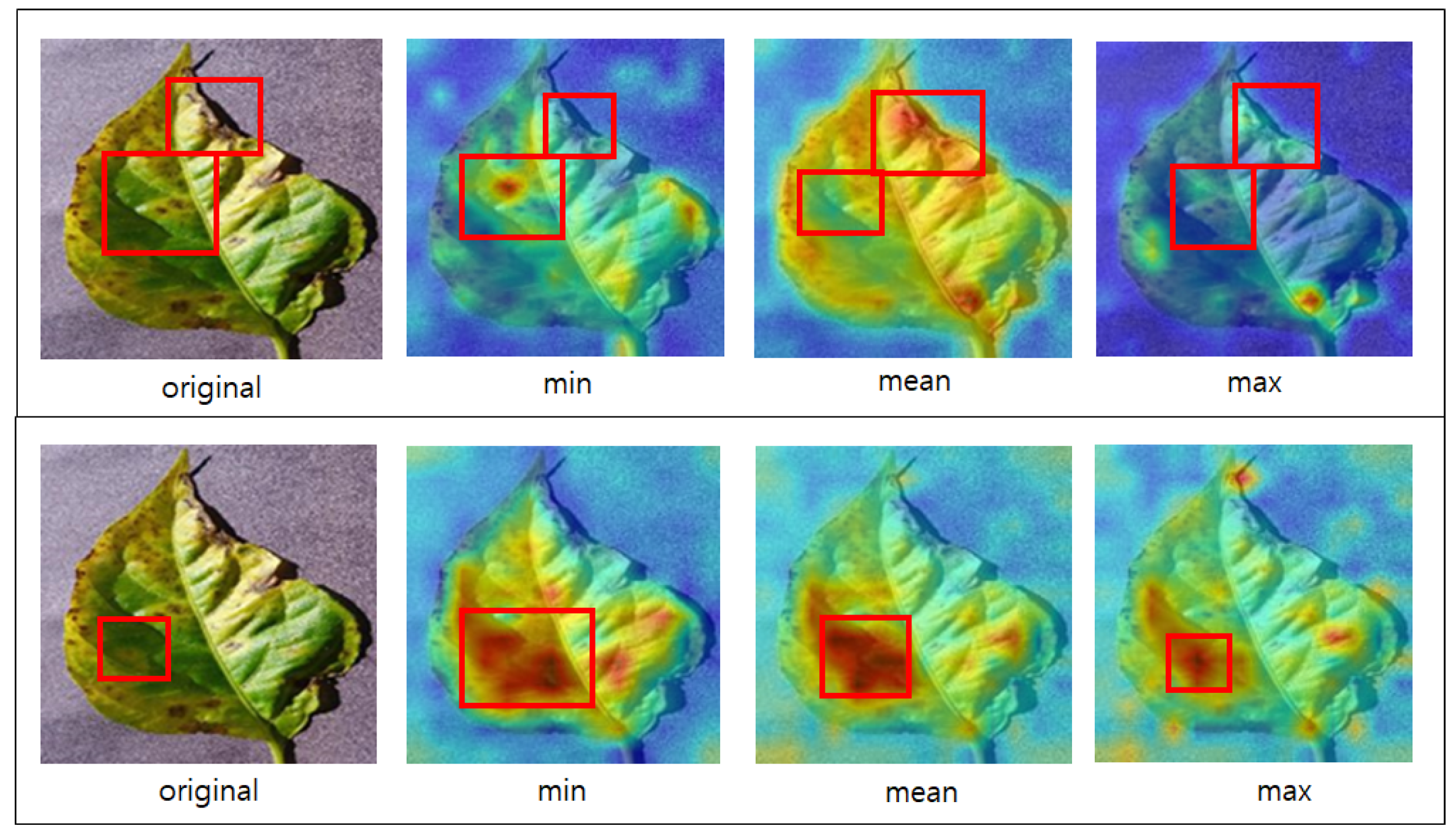
To better understand the six models and crop diseases, we loaded the weights of the model that achieved the highest F1 score according to Table 5 and visualized the feature maps. The feature maps represent the process of extracting patterns as the models pass through the layers and capture the characteristics of crop diseases. By examining the feature maps, we saw how the models perceived the features of agricultural pests and diseases. The red bounding box highlights regions within the feature map where the disease object is prominently represented, providing an analytical visualization of its salient characteristics.

Figure 7 shows the images from which the feature maps were extracted using the VGGNet and ResNet models. The VGGNet model appears to focus on the edges of the leaves as it progresses through the convolution layers. Additionally, since VGGNet employs only 16 layers, its feature maps maintain the shape of the original image even after passing through the convolutions, unlike those of the other models. In contrast, the ResNet model emphasizes the bottom of the leaves to locate the disease. The first right row in Figure 7 shows images from the higher layers of the ResNet model. In all three images, the disease is observable in the exact location. Although the VGGNet and ResNet models identified the disease in different locations, both accurately recognized the objects associated with the disease.

Figure 8 shows the images from which the feature maps were extracted using the DenseNet model. Unlike the previous two models, the DenseNet model detects the disease in the center of the leaves. It can be observed that the DenseNet model consistently maintains the recognition of disease patterns as it passes through the dense blocks without losing them. Similar to DenseNet, the EfficientNet model recognizes the disease in the exact location. The EfficientNet model appears to have uniform intensity in the images and detects the brightness of the background more rapidly than the previous three models.

Figure 9 shows an image from which the attention map was extracted using the ViT model and Deit, specifically the multihead attention’s minimum (min), mean, and maximum (max) values. The above attention map corresponds to the ViT model, and the one below corresponds to the DeiT model. When the mean value is emphasized, each head focuses on a different position, allowing the model to recognize diseases at the edges of the image. However, the minimum and maximum values are concentrated in the localized areas of the image. The attention map of DeiT exhibits a pattern different from that of ViT. ViT’s attention map shows a wide distribution when emphasizing the mean value but that of DeiT shows variations in distribution based on the minimum, mean, and maximum values but still focuses on common areas. By visually examining the image, the model may seem to focus on normal leaf regions rather than diseased parts. However, upon closer examination of the attention maps for mean and maximum values, it becomes apparent that the model recognizes the diseases.

7. Discussion and Conclusions

In this section, we compare the proposed approach with prior methods using the same crop disease data from the PlantVillage dataset employed in our experiments.

Table 7. Comparison of the performance of the proposed model with that of other models on the PlantVillage dataset.

Type	Disease Name	Method	Performance
ML-Based [13]	Pepper Bacterial Spot	K-Nearest Neighbor (KNN)	80.5%
	Pepper Healthy	Naïve Bayes (NB)	89.83%
	Potato Early Blight	Decision Tree (DT)	79.5%
	Potato Late Blight	K-Nearest Neighbor (KNN)	71%
	Potato Healthy	Artificial Neural Networks (ANNs)	51.61%
DL-based	Potato Early Blight	DenseNet [18]	97.8%
	Potato Late Blight		97.6%
	Tomato (10 classes)	Darknet53 + Densenet201 + EfficientNetb0 [40]	98.08%
Proposed	Pepper (2 classes)	ResNet	98.28%
	Potato (2 classes)	DenseNet	99.39%
	Tomato (10 classes)	ViT	99.17%

presents a comparative analysis between our method and prior methods leveraging the same dataset. As shown in Table 7, ML-based models exhibited a notable decline in performance on identical crop data, while DL-based models demonstrated performance comparable to or marginally superior to our results. However, our study employed a unified model capable of addressing multiple crop types simultaneously, unlike prior studies that optimized distinct models for individual crops. Naturally, such crop-specific models achieved higher performance. Moreover, while the PlantVillage dataset includes only leaf images, our study incorporated both leaf and fruit images, which introduced additional complexity but enhanced the model’s generalizability. If separate classification tasks had been conducted for leaf and fruit images, our model’s performance would likely have improved further. Despite these challenges, our model achieved nearly 99% accuracy, underscoring its effectiveness across diverse data types.

This study analyzed data augmentation techniques to develop a method that enables deep learning models to perform disease diagnosis efficiently. A novel dataset comprising 24 classes significantly enhanced the model’s generalization capability across diverse crop types. The integration of geometric transformations and color space modifications resulted in deep learning architectures, including VGGNet, ResNet, DenseNet, EfficientNet, ViT, and DeiT, achieving F1 scores exceeding 98%. Furthermore, our approach emphasizes the potential for reducing energy consumption and carbon emissions by employing a single model for multiple crop types, contributing to sustainable agriculture through scalable disease detection methods. However, reliance on image data alone imposes limitations on broader applicability. To address this, future research will explore integrating image and text data to develop multimodal classification systems, further enhancing robustness and versatility.

References

1. Piscicelli, L. The sustainability impact of a digital circular economy. Curr. Opin. Environ. Sustain. 2023, 61, 101251. [Google Scholar] [CrossRef]
2. Andersen, A.D.; Frenken, K.; Galaz, V.; Kern, F.; Klerkx, L.; Mouthaan, M.; Piscicelli, L.; Schor, J.B.; Vaskelainen, T. On digitalization and sustainability transitions. Environ. Innov. Soc. Transit. 2021, 41, 96–98. [Google Scholar] [CrossRef]
3. Moore, D.; Robson, G.D.; Trinci, A.P. 21st Century Guidebook to Fungi; Cambridge University Press: Cambridge, UK, 2020. [Google Scholar]
4. Tang, F.H.; Malik, A.; Li, M.; Lenzen, M.; Maggi, F. International demand for food and services drives environmental footprints of pesticide use. Commun. Earth Environ. 2022, 3, 272. [Google Scholar] [CrossRef]
5. Mäkitie, T.; Hanson, J.; Damman, S.; Wardeberg, M. Digital innovation’s contribution to sustainability transitions. Technol. Soc. 2023, 73, 102255. [Google Scholar] [CrossRef]
6. Caserta, R.; Teixeira-Silva, N.; Granato, L.; Dorta, S.; Rodrigues, C.; Mitre, L.; Yochikawa, J.; Fischer, E.; Nascimento, C.; Souza-Neto, R.; et al. Citrus biotechnology: What has been done to improve disease resistance in such an important crop? Biotechnol. Res. Innov. 2019, 3, 95–109. [Google Scholar] [CrossRef]
7. Agarwal, M.; Gupta, S.K.; Biswas, K. Development of Efficient CNN model for Tomato crop disease identification. Sustain. Comput. Inform. Syst. 2020, 28, 100407. [Google Scholar] [CrossRef]
8. Hughes, D.; Salathé, M. An open access repository of images on plant health to enable the development of mobile disease diagnostics. arXiv 2015, arXiv:1511.08060. [Google Scholar]
9. Dhiman, P.; Kukreja, V.; Manoharan, P.; Kaur, A.; Kamruzzaman, M.; Dhaou, I.B.; Iwendi, C. A novel deep learning model for detection of severity level of the disease in citrus fruits. Electronics 2022, 11, 495. [Google Scholar] [CrossRef]
10. Verma, B.; Zhang, L.; Stockwell, D. Roadside Video Data Analysis: Deep Learning; Springer: Berlin/Heidelberg, Germany, 2017. [Google Scholar]
11. Luaibi, A.R.; Salman, T.M.; Miry, A.H. Detection of citrus leaf diseases using a deep learning technique. Int. J. Electr. Comput. Eng. 2021, 11, 1719. [Google Scholar] [CrossRef]
12. Jagtap, S.T.; Phasinam, K.; Kassanuk, T.; Jha, S.S.; Ghosh, T.; Thakar, C.M. Towards application of various machine learning techniques in agriculture. Mater. Today Proc. 2022, 51, 793–797. [Google Scholar] [CrossRef]
13. Appalanaidu, M.V.; Kumaravelan, G. Classification of Plant Disease using Machine Learning Algorithms. In Proceedings of the 2024 Sixth International Conference on Computational Intelligence and Communication Technologies (CCICT), Sonepat, India, 19–20 April 2024; pp. 1–7. [Google Scholar]
14. Dananjayan, S.; Tang, Y.; Zhuang, J.; Hou, C.; Luo, S. Assessment of state-of-the-art deep learning based citrus disease detection techniques using annotated optical leaf images. Comput. Electron. Agric. 2022, 193, 106658. [Google Scholar] [CrossRef]
15. Dhaka, V.S.; Meena, S.V.; Rani, G.; Sinwar, D.; Ijaz, M.F.; Woźniak, M. A survey of deep convolutional neural networks applied for prediction of plant leaf diseases. Sensors 2021, 21, 4749. [Google Scholar] [CrossRef]
16. Petchiammal; Kiruba, B.; Murugan; Arjunan, P. Paddy doctor: A visual image dataset for automated paddy disease classification and benchmarking. In Proceedings of the 6th Joint International Conference on Data Science & Management of Data (10th ACM IKDD CODS and 28th COMAD), Mumbai, India, 4–7 January 2023; pp. 203–207. [Google Scholar]
17. Liu, J.; Wang, M.; Bao, L.; Li, X. EfficientNet based recognition of maize diseases by leaf image classification. J. Phys. Conf. Ser. 2020, 1693, 012148. [Google Scholar] [CrossRef]
18. Mahum, R.; Munir, H.; Mughal, Z.U.N.; Awais, M.; Sher Khan, F.; Saqlain, M.; Mahamad, S.; Tlili, I. A novel framework for potato leaf disease detection using an efficient deep learning model. Hum. Ecol. Risk Assess. Int. J. 2023, 29, 303–326. [Google Scholar] [CrossRef]
19. Simonyan, K.; Zisserman, A. Very deep convolutional networks for large-scale image recognition. arXiv 2014, arXiv:1409.1556. [Google Scholar]
20. He, K.; Zhang, X.; Ren, S.; Sun, J. Deep residual learning for image recognition. In Proceedings of the IEEE Conference on Computer Vision and Pattern Recognition, Las Vegas, NV, USA, 27–30 June 2016; pp. 770–778. [Google Scholar]
21. Huang, G.; Liu, Z.; Van Der Maaten, L.; Weinberger, K.Q. Densely connected convolutional networks. In Proceedings of the IEEE Conference on Computer Vision and Pattern Recognition, Honolulu, HI, USA, 21–26 July 2017; pp. 4700–4708. [Google Scholar]
22. Tan, M.; Le, Q. Efficientnet: Rethinking model scaling for convolutional neural networks. In Proceedings of the International Conference on Machine Learning, Long Beach, CA, USA, 9–15 June 2019; pp. 6105–6114. [Google Scholar]
23. Dosovitskiy, A.; Beyer, L.; Kolesnikov, A.; Weissenborn, D.; Zhai, X.; Unterthiner, T.; Dehghani, M.; Minderer, M.; Heigold, G.; Gelly, S.; et al. An image is worth 16 × 16 words: Transformers for image recognition at scale. arXiv 2020, arXiv:2010.11929. [Google Scholar]
24. Touvron, H.; Cord, M.; Douze, M.; Massa, F.; Sablayrolles, A.; Jégou, H. Training data-efficient image transformers & distillation through attention. In Proceedings of the International Conference on Machine Learning, Virtual, 18–24 July 2021; pp. 10347–10357. [Google Scholar]
25. Jun, B.; Kim, I.; Shin, J.; Kwon, H. Development of landscape conservation value map of Jeju island, Korea for integrative landscape management and planning using conservation value of landscape typology. PeerJ 2021, 9, e11449. [Google Scholar] [CrossRef] [PubMed]
26. Henderson, D.; Hamernik, R. Impulse noise: Critical review. J. Acoust. Soc. Am. 1986, 80, 569–584. [Google Scholar] [CrossRef] [PubMed]
27. Kassam, S.A. Signal Detection in Non-Gaussian Noise; Springer Science & Business Media: Berlin/Heidelberg, Germany, 2012. [Google Scholar]
28. Meyers, R.A. Encyclopedia of Physical Sciences and Technology; Academic Press: San Diego, CA, USA, 1992. [Google Scholar]
29. Hasinoff, S.W. Photon, Poisson Noise. Comput. Vis. Ref. Guide 2014, 4, 1. [Google Scholar]
30. Boyat, A.K.; Joshi, B.K. A review paper: Noise models in digital image processing. arXiv 2015, arXiv:1505.03489. [Google Scholar] [CrossRef]
31. Shao, H.; Beaulieu, N.C. Block coding for impulsive laplacian noise. In Proceedings of the 2010 IEEE International Conference on Communications, Cape Town, South Africa, 23–27 May 2010; pp. 1–6. [Google Scholar]
32. Gedraite, E.S.; Hadad, M. Investigation on the effect of a Gaussian Blur in image filtering and segmentation. In Proceedings of the ELMAR-2011, Zadar, Croatia, 14–16 September 2011; pp. 393–396. [Google Scholar]
33. Jhawar, J.; Morris, R.G.; Guttal, V. Deriving mesoscopic models of collective behavior for finite populations. In Handbook of Statistics; Elsevier: Amsterdam, The Netherlands, 2019; Volume 40, pp. 551–594. [Google Scholar]
34. Deng, J.; Dong, W.; Socher, R.; Li, L.J.; Li, K.; Fei-Fei, L. Imagenet: A large-scale hierarchical image database. In Proceedings of the 2009 IEEE Conference on Computer Vision and Pattern Recognition, Miami, FL, USA, 20–25 June 2009; pp. 248–255. [Google Scholar]
35. Krizhevsky, A.; Sutskever, I.; Hinton, G.E. ImageNet classification with deep convolutional neural networks. In Proceedings of the 26th Annual Conference on Neural Information Processing Systems (NIPS 2012), Lake Tahoe, NV, USA, 3–6 December 2012. [Google Scholar]
36. Szegedy, C.; Liu, W.; Jia, Y.; Sermanet, P.; Reed, S.; Anguelov, D.; Erhan, D.; Vanhoucke, V.; Rabinovich, A. Going deeper with convolutions. In Proceedings of the IEEE Conference on Computer Vision and Pattern Recognition, Boston, MA, USA, 7–12 June 2015; pp. 1–9. [Google Scholar]
37. Zhang, Z.; Sabuncu, M. Generalized cross entropy loss for training deep neural networks with noisy labels. In Proceedings of the 32nd Conference on Neural Information Processing Systems (NeurIPS 2018), Montreal, QB, Canada, 3–8 December 2018. [Google Scholar]
38. Kingma, D.P.; Ba, J. Adam: A method for stochastic optimization. arXiv 2014, arXiv:1412.6980. [Google Scholar]
39. Gotmare, A.; Keskar, N.S.; Xiong, C.; Socher, R. A closer look at deep learning heuristics: Learning rate restarts, warmup and distillation. arXiv 2018, arXiv:1810.13243. [Google Scholar]
40. Chouchane, A.; Ouamanea, A.; Himeur, Y.; Amira, A. Deep learning-based leaf image analysis for tomato plant disease detection and classification. In Proceedings of the 2024 IEEE International Conference on Image Processing (ICIP), Abu Dhabi, United Arab Emirates, 27–30 October 2024; pp. 2923–2929. [Google Scholar]
Figure 1. Geographic map of the data acquisition area (red pinpoint: citrus, blue pinpoint: kiwi).
Bdcc 09 00008 g001
Figure 2. Sample images of data collected from farmland.
Bdcc 09 00008 g002
Figure 3. Sample images with multiplicative Gaussian noise.
Bdcc 09 00008 g003
Figure 4. Dataset image samples. The red box indicates samples with minimal color contrast, making disease feature identification difficult. The blue box highlights samples with strong shadows caused by sunlight, which can introduce noise and obscure disease patterns.
Bdcc 09 00008 g004
Figure 5. Image with color jitter data augmentation method.
Bdcc 09 00008 g005
Figure 6. The overall workflow of the proposed network architecture.
Bdcc 09 00008 g006
Figure 7. The left side shows the feature map obtained with VGGNet, and the right side shows the feature map obtained with ResNet.
Bdcc 09 00008 g007
Figure 8. The left side shows the feature map obtained with DenseNet, and the right side shows the feature map obtained with EfficientNet.
Bdcc 09 00008 g008
Figure 9. The top image shows the feature map obtained with ViT, while the bottom image shows the feature map obtained with DeiT.
Bdcc 09 00008 g009