Article

Stock Trend Prediction with Machine Learning: Incorporating Inter-Stock Correlation Information through Laplacian Matrix

1
LSEC, ICMSEC, NCMIS, Academy of Mathematics and Systems Science, Chinese Academy of Sciences, Beijing 100190, China
2
School of Mathematical Sciences, University of Chinese Academy of Sciences, Beijing 100049, China
*
Author to whom correspondence should be addressed.
Big Data Cogn. Comput. 2024, 8(6), 56; https://doi.org/10.3390/bdcc8060056
Submission received: 12 April 2024 / Revised: 25 May 2024 / Accepted: 28 May 2024 / Published: 30 May 2024
(This article belongs to the Special Issue Big Data Analytics and Edge Computing: Recent Trends and Future)

Abstract

:
Predicting stock trends in financial markets is of significant importance to investors and portfolio managers. In addition to a stock’s historical price information, the correlation between that stock and others can also provide valuable information for forecasting future returns. Existing methods often fall short of straightforward and effective capture of the intricate interdependencies between stocks. In this research, we introduce the concept of a Laplacian correlation graph (LOG), designed to explicitly model the correlations in stock price changes as the edges of a graph. After constructing the LOG, we will build a machine learning model, such as a graph attention network (GAT), and incorporate the LOG into the loss term. This innovative loss term is designed to empower the neural network to learn and leverage price correlations among different stocks in a straightforward but effective manner. The advantage of a Laplacian matrix is that matrix operation form is more suitable for current machine learning frameworks, thus achieving high computational efficiency and simpler model representation. Experimental results demonstrate improvements across multiple evaluation metrics using our LOG. Incorporating our LOG into five base machine learning models consistently enhances their predictive performance. Furthermore, backtesting results reveal superior returns and information ratios, underscoring the practical implications of our approach for real-world investment decisions. Our study addresses the limitations of existing methods that miss the correlation between stocks or fail to model correlation in a simple and effective way, and the proposed LOG emerges as a promising tool for stock returns prediction, offering enhanced predictive accuracy and improved investment outcomes.

1. Introduction

The accurate prediction of stock trends has long been a vital focus of financial analysis and investment decision making. In today’s volatile and increasingly complex financial market, precise stock price forecasts can significantly improve investment strategies, risk management, and portfolio optimization.
The application of advanced computational methods, coupled with the abundance of financial data, has facilitated the evolution of intricate predictive models adept at capturing the hidden patterns within stock price fluctuations. Over time, a spectrum of techniques, spanning from classical time series analysis to modern machine learning algorithms, has been deployed to address the formidable challenge of forecasting stock trends (see Section 2).
Correlation is a widely employed metric in the realm of financial markets. It has been a fundamental component in financial analysis dating back to Markowitz’s pioneering portfolio theory [1], where the goal of minimizing the variance of investment portfolios was achieved by calculating the correlation between different asset returns. Markowitz’s groundbreaking work established the basis for modern portfolio theory (MPT) and earned him the Nobel Prize in 1990. To this day, financial analysts routinely conduct assessments of correlations among a wide range of asset returns. These assessments include the returns of different sectors, industries, and indices from a macroscopic perspective, as well as the correlations between individual stocks from a more microscopic viewpoint. It is evident that correlation can furnish vital information. For example, quantifying the correlation between industry sectors may carry important implications for asset pricing and sector diversification [2]. The correlation between stock indices over time reflects the cyclical characteristics of the real sector economy [3].
In the task of stock trend prediction, the integration of correlation information between stock prices also holds significant importance. Notably, various stocks exhibit discernible positive or negative correlations, as depicted in Figure 1. This correlation information presents an opportunity to enhance prediction accuracy when forecasting stock returns. Some correlations can be rationalized by stocks belonging to the same industry, exemplified by the strong positive correlation between 000825.SZ (Shanxi Taigang Stainless Steel, Taiyuan, China) and 000898.SZ (Angang Steel Company Limited, Anshan, China), both representing steel companies, with a Pearson correlation coefficient of 0.90 for the period from 1 January 2016 to 30 June 2020. In some instances, the relationships between strongly correlated stocks are less intuitive. For example, 600027.SH (Huadian Power International Corporation Limited, Jinan, China) and 002230.SZ (iFLYTEK, Hefei, China) are different types of companies, which belong to distinct industries, and are not even listed on the same exchange. Intuitively, the correlation coefficient should be very close to 0 as they lack evident fundamental connections. However, they exhibit a substantial negative correlation. Their Pearson correlation coefficient for the period from 1 January 2016 to 30 June 2020 is −0.77. This diversity in correlation sources, some grounded in fundamental factors while others not, underscores the motivation to devise an approach that captures stock correlations solely through historical price data, without relying on fundamental properties.
In this paper, we delve into the prediction of stock returns using neural networks with an emphasis on leveraging graph-based methodologies. We use the information of correlation between stock prices in a quite simple but effective way. We built a graph for the chosen stock pool in which correlations serve as edge weights and stock return predictions are represented as signals on the graph. Utilizing the Laplacian matrix of this graph, we computed the signal’s smoothness. By incorporating this smoothness measure into the loss function, our model accommodates the correlation between stock prices. These techniques have shown promising results in capturing the interdependencies and correlations among stocks within a dynamic market environment. By exploiting the inherent structure of financial markets, as encapsulated by stock correlation graphs, we endeavor to augment the precision and robustness of predictions concerning stock returns.
To demonstrate the effectiveness of our proposed approach, we conduct extensive experiments on two highly representative stock pools in the Chinese stock market: the constituent stocks of the CSI100 and CSI300 indices. These stock pools provide fertile ground for evaluating the practical applicability of our method, given their status as reflections of the most influential companies traded in the Shanghai and Shenzhen stock exchanges. Through comprehensive analysis and rigorous evaluation, our method exhibits a higher information coefficient (IC) relative to conventional neural network methods, resulting in superior annualized returns and an enhanced information ratio (IR).
The remaining structure of this paper is organized as follows. Section 2 provides an overview of related work in stock price prediction and portfolio investment methodologies. Section 3 gives a detailed explanation of our problem and the definition of the target to be predicted. In Section 4, we present the methodology underpinning our graph-based approach to stock price trend prediction. Section 5 outlines our experimental setup and presents the results and analysis. We conclude in Section 6 by summarizing our findings, discussing their implications, and providing suggestions for future research.

2. Related Work

Stock price prediction has been a subject of enduring interest within the fields of finance and machine learning. Numerous approaches have been explored to enhance predictive accuracy and inform investment strategies. This section provides an overview of the pertinent literature and research efforts.
The predicting techniques used in the literature can be categorized into two principal classes: statistical methods and artificial intelligence models [4].

2.1. Statistical Methods

Statistical methods in investment do not consider real-world events or fundamental analysis [5] but purely employ historical data, such as prices, trading volumes, and other available data to predict price trends that are believed to persist into the future [6]. It is also called technical analysis. The simplest statistical methods used in the early days include simple moving average (SMA), weighted moving average (WMA) [7], and exponential smoothing [8]. SMA computes the unweighted mean of a specific number of preceding data points to estimate the value for the subsequent day. In contrast, WMA employs a weighted average of prior data to forecast future values. Exponential smoothing, on the other hand, utilizes a smoothing constant denoted as α to iteratively refine the prediction value based on the preceding forecast, with the aim of optimizing prediction accuracy in relation to the most recent prediction. Although these techniques provide a foundational understanding, the intricacies of stock markets often necessitate more sophisticated models. The autoregressive integrated moving average (ARIMA) [9] model emerges as a more complicated and robust statistical approach for stock price forecasting. In the ARIMA model, the future value of the stock price is a linear combination of past prices and past errors. Additionally, the generalized autoregressive conditional heteroskedasticity (GARCH) model is often used for forecasting stock market volatility [10].

2.2. Artificial Intelligence Models

Although these advanced statistical models, such as ARIMA and GARCH, are better equipped to capture the complexities of stock markets, the linearity of these traditional statistical models hampers the prediction performances in the case of sudden rise or fall of stock prices [8]. To better extract profitable patterns from historical stock data, artificial intelligence-based methods including machine learning methods and deep learning methods are vital.

2.2.1. Machine Learning Methods

The decision tree algorithm is often used for stock trend prediction. Nair et al. build a C4.5 decision tree to select the relevant features and design a rough set-based system from the extracted features to predict the next-day trend [11]. Wang and Chan introduce a two-layer bias decision tree with technical indicators to create a rule that decides to buy or not buy [12]. Support vector machines (SVMs) are also successfully applied in the time series prediction domain due to their ability to achieve a high generalization performance and testing accuracy [13]. Tay et al. introduce the application of SVM for financial time series forecasting and show effective applications in the stock markets [14]. Grigoryan proposes an SVM model with independent component analysis (ICA) for stock market prediction [13].
Compared with these single classifiers, classifier ensembles have been shown to perform better [15]. Khaidem et al. show the applications of random forest in stock trend prediction. The learning model used is an ensemble of multiple decision trees and achieves impressive and robust results [16]. Tsai et al. consider the hybrid methods of majority voting and bagging. The results show that multiple classifiers outperform single classifiers in terms of prediction accuracy and returns on investment [17].

2.2.2. Deep Learning Methods

In addition to the traditional machine learning methods mentioned above, deep learning techniques have received widespread attention in various fields, including the investment field. The simplest model is multi-layer perceptron (MLP) [18,19,20]. To further model the long-term dependency in the time domain, recurrent neural networks (RNN), especially long short-term memory (LSTM) networks, have also been employed in financial prediction [21,22,23]. In particular, Nelson et al. study the usage of LSTM networks on the prediction of future trends of stock prices based on the price history, alongside technical analysis indicators [22]. Chen et al. demonstrate the power of LSTM in stock market prediction in China [21]. Roondiwala et al. present an RNN and LSTM approach to predict stock market indices [23].
These methods primarily focus on modeling the time series of individual stocks in isolation, often disregarding the interdependencies and correlations between stocks. It is essential to recognize that individual stocks are interconnected, and more useful patterns appear when the relationship between stocks is considered. Researchers explore the relationship between subjects as prior knowledge to improve the fitting ability of deep learning models [24]. To mine the cross-stock shared information and improve the stock trend forecasting performance, many cross-stock methods employ the graph neural network (GNN) [25]. Li et al. propose an LSTM relational graph convolutional network to model the connection among stocks with their correlation matrix. They build the connection between two stocks when the absolute value of their correlation is above a threshold [26]. Long et al. utilize the knowledge graph and graph embedding techniques to select the relevant stocks of the target for constructing the market and trading information [27]. Wu et al. treat trading days as nodes and use graph embeddings to represent the association between time points as input and use node weights as a priori knowledge to enhance the learning of temporal attention [28].

3. Problem Formulation

This section elucidates the problem statements and related concepts. Because the exact price of a stock is extremely hard to predict accurately [29], we predict the stock price movement instead.
Definition 1
(Stock returns). It is common to define the stock price trend as stock returns, namely the change rate of the stock price at the next time step. If we consider the close price of stock i at time t as p i t , then the stock return of stock i at time t is defined as the following:
r i t = p i t + 2 p i t + 1 p i t + 1 .
Much of the literature in academic research use P t + 1 P t P t to represent the returns r t at time t. However, the reason for using the change rate from time t + 1 to time t + 2 rather than that from time t to time t + 1 lies in the fact that, when making investments, knowledge of the close price of time t implies that the stock market has already closed on that day, and hence purchasing stocks at that close price of day t is unrealistic. In practice, most asset management companies such as hedge funds or proprietary trading firms use the price of the next time period, because we cannot buy at the current close price in reality, and the use of price for the next time will result in a more realistic accurate rate of return. It is sometimes called the actual return [30,31]. Therefore, it becomes imperative to forecast the change rate for the next day, which would enable us to buy stocks at the close price of day t + 1 and eventually sell them on day t + 2 .
Problem 1
(Stock Trend Prediction). Given a set of stock features of stock i at time t, the objective of stock trend prediction is to forecast the stock return r i t .

4. Our Framework

In this section, we present fundamental concepts and our framework. We begin by introducing the correlation matrix, followed by an explanation of the graph Laplacian. Finally, we outline the construction of our Laplacian correlation graph (LOG) and the design of the associated loss function to optimize neural network parameters.

4.1. Correlation Matrix

Let r i t denote the return of stock i at time t. Then, given the window size of a time period T, we can calculate the Pearson’s correlation coefficient ρ i j between any stock pairs. First, we calculate the mean and the variance value of the stock return of stock i during this time period as follows:
r ¯ i = 1 T t = 0 T r i t ,
Var i = 1 T t = 0 T r i t r ¯ i 2 .
Then, we define the Pearson’s correlation coefficient ρ i j between stock i and stock j as follows:
ρ i j = 1 T t = 0 T r i t r ¯ i r j t r ¯ j Var i · Var j .
Let W R n × n , where n is the number of stocks in the stock pool and W i j = ρ i j , then W is the correlation matrix of the stock pool under investigation.

4.2. Laplacian Matrices of Graphs

Let G = ( V , E ) be a graph on n vertices, with its vertex set V = V ( G ) = { v 1 , , v n } and edge set E = E ( G ) = { e 1 , , e m } . Suppose G is an undirected graph without loops or multiple edges.
We can then define an adjacency matrix A ( G ) and a degree matrix D ( G ) as follows:
A i j = 0 if ( v i , v j ) E , 1 if ( v i , v j ) E ,
and D = diag ( D 1 , , D n ) , where D i is the degree of vertex i, D i = j = 1 n A i j . The adjacency matrix is a means of representing which vertices of a graph are adjacent to which other vertices [32]. And the degree of a vertex reflects the number of other vertices it is connected to.
Given A ( G ) and D ( G ) , the Laplacian matrix L ( G ) is defined as L ( G ) = D ( G ) A ( G ) . Let X = ( x 1 , , x n ) be a signal on V, the Laplacian matrix G has the following quadratic form property:
x T L x = i , j L i j x i x j = i = 1 n D i x i 2 i j A i j x i x j = 1 2 i = 1 n D i x i 2 2 i j A i j x i x j + j = 1 n D j x j 2 = 1 2 j i A i j x i 2 2 i j A i j x i x j + i j A j i x j 2 = 1 2 i j A i j x i 2 2 x i x j + x j 2 = 1 2 i j A i j x i x j 2 = 1 2 ( v i , v j ) E ( x i x j ) 2 .
Consider a more general situation where edges have weights. The above is a special case where all edge weights are 0 or 1. Define the weight matrix W = ( w i j ) , where w i j is the weight of edge ( v i , v j ) . The W is similar to the adjacency matrix but with arbitrary values. We similarly define the degree matrix D = diag ( D 1 , , D n ) , where D i = j = 1 n w i j , let L ( G ) = D ( G ) W ( G ) , we have the following quadratic form property by simply substitute W for A in the above formula:
x T L x = 1 2 i j W i j x i x j 2
This quadratic form can be used to measure the smoothness of the signal X on the graph. The closer the signal values on the two vertices connected by edges with higher weights, the smaller the quadratic form, and the smoother the signal. Through this property, the Laplacian matrix connects the similarity of two vertices with the similarity of signals on the vertices. This is the main idea we will use to formulate that positively correlated stocks will have similar price trends in the future.

4.3. Laplacian Correlation Graph

We consider a correlation-based graph G = ( V , E ) . Individual stock is considered as a node. It is common practice to construct stock market graphs using Pearson’s correlation coefficient [33], as this can measure the similarity between nodes. Both weighted and unweighted edges can be used. For an unweighted graph, there will be an edge between the node i and j if ρ i j ρ thres  [26].
For weighted graphs, various methods can be employed to determine weights based on the correlation between stock pairs. One way is to take the absolute value, w i j = | ρ i j |  [34]. However, this method has the limitation of assigning a positive similarity to negatively correlated stocks. Alternatively, the correlation can be transformed into a distance measure, w i j = 2 ( 1 ρ i j )  [35]. This distance is inversely related to the correlation coefficient, and when the correlation is close to 1, this distance is too small to display the close similarity, thus this is an improper method for our use. In our work, we directly use the correlation coefficients as the weight of edges without transformation. This approach ensures that in subsequent calculations of the Laplacian matrix quadratic form, greater weights are automatically assigned to the differences between stocks with higher similarities. The correlation coefficients are dynamically updated by training sets because our dataset is rolled forward for six months each time.
To build a LOG, we first apply a modification to the correlation matrix to form a weight matrix that is more compatible with graph theory. Let W ˜ denote the adjusted weight matrix, where W ˜ is defined as follows:
W ˜ i j = 0 if i = j , W i j if i j ,
where W ˜ is symmetric because W is symmetric.
Let G = ( S , E , W ˜ ) be a weighted graph where S denotes the stock pool and E represents the set of stock pairs. We define a diagonal matrix of node degrees D as follows:
D i j = k i W ˜ i k if i = j , 0 if i j ,
and the graph Laplacian is defined as
L = D W ˜ , L i j = k i W ˜ i k if i = j , W ˜ i j if i j .
This graph is formed based on correlations and draws inspiration from the Laplacian matrix, thus referred to as a Laplacian correlation graph (LOG). The graph Laplacian can be used to measure the smoothness of a signal on a graph.
For a signal on a graph x : S R , x R n , x i is the signal on vertex i, and the smoothness of x can be measured with a quadratic form of the graph Laplacian,
x T L x = 1 2 i j W ˜ i j x i x j 2 .
Inspired by this property of graph Laplacian, we can design the loss function to characterize stock correlation.

4.4. Training Loss Design

The loss function consists of two parts after we construct the LOG.
Improve estimate. First, we choose a base model, such as LSTM. The experiments we conduct in Section 5 choose five base models. The base model uses the mean squared error (MSE) loss function that depicts the accuracy of the original neural network.
L 1 ( θ ) = t T MSE t = t T i S t ( r ^ i t r i t ) 2 | S t | .
Here, T is the set of trading days in the training period; MSE t is the MSE loss on trading day t; S t is the stock pool considered on trading day t; r ^ i t and r i t represent the prediction and the ground truth of return of stock i at day t, respectively; θ is the parameter of the neural network in the base model.
Maintain correlation. Then, we add our LOG. We conduct a second term to evaluate the prediction of correlations between stocks. We refer to this term as the correlation penalty.
L 2 ( θ ) = t T i , j S t W ˜ i j ( r ^ i t r ^ j t ) 2 2 | S t | .
Here, W ˜ i j is the entry ( i , j ) of the adjusted weight matrix. It represents the correlation between stock i and stock j; therefore, we employ it as a weight coefficient. Although some studies indicate that correlations may not be fully maintained in the long run, researchers found that short-term correlations of assets exhibit relatively little change. Let W t = β W t 1 + F ( ε t 1 ) be an autoregression model to formulate the dynamic evolution of correlations. Empirical results [36,37] show that the β is always within [ 0.9 , 1 ] , thus showing that the correlation of adjacent time periods is very close. Therefore. it is expected that stocks with positive correlations in the past will maintain the correlation in the near future. The greater the correlation coefficient between two stocks, the more similar their future trends will be. This term can be computed in a vectorized manner by the Laplacian matrix of the graph, and the matrix form can improve computational efficiency. Let r ^ t = ( r ^ 1 t , , r ^ | S t | t ) be the prediction vector on day t. The second loss term can be then formulated as
L 2 ( θ ) = t T 1 | S t | ( r ^ t ) L ( r ^ t ) .
By formulating the loss into the matrix form, it will save a lot of time compared to calculating term by term, thus improving computational efficiency. It also provides a simpler model representation. The construction of the correlation graph, as well as the calculation of its Laplacian matrix, leads to the quadratic form, which automatically assigns a larger weight to the difference of stocks with higher similarities.
The total loss function is
L ( θ ) = L 1 ( θ ) + λ L 2 ( θ ) .
Here, λ is a hyper-parameter that regulates the effect of the correlation penalty. The set of neural network parameters θ is iteratively updated using Adam algorithms to solve the following optimization problem:
θ 0 = arg min θ Θ L ( θ ) .
Figure 2 shows the framework of our LOG structure. Algorithm 1 shows the overall algorithm.
Algorithm 1 LOG framework.
Input: Stock pool S , Features F, base model M ( θ ) , n e p o c h ;
Output: M ( θ ) ;
 Calculate W , W ˜ , D , L
for all i = 1 , 2 , , n e p o c h  do
   R ^ = M ( F ) ;
   L 1 ( θ ) = MSE ( R ^ , R ) ;
   L 2 ( θ ) = Mean ( R ^ T L R ^ ) ;
   L ( θ ) = L 1 ( θ ) + λ L 2 ( θ ) ;
  Optimizing algorithms to update θ by minimizing L ( θ ) ;
end for
return  M ( θ ) .

5. Experiments

We conduct multiple sets of experiments with real-world data to validate the effectiveness of our proposed method in practical applications.

5.1. Datasets

Stock pools. We evaluate our method on two highly representative stock pools in the Chinese stock market: constituent stocks of CSI100 and CSI300 indices. CSI100 and CSI300 consist of the top 100 and top 300 stocks traded in the Shanghai and Shenzhen stock exchanges. Therefore, CSI100 reflects the performances of the most influential large-cap A-shares market, whereas CSI300 is regarded as the Chinese counterpart of the S&P 500 and serves as a comprehensive gauge of the overall performance of the Chinese stock market.
Stock features. We use the stock features of Alpha158 in the open-source, AI-oriented quantitative investment platform Qlib [38]. Alpha158 contains 158 features, or, in quantitative investment terms, factors. All of these factors are derived from six fundamental components of stock data, namely, the opening price, closing price, highest price, lowest price, volume-weighted average price (VWAP), and trading volume for each trading day, as commonly employed in quantitative investment analysis.

5.2. Data Processing

We conduct several pre-processing steps for the data before training. There are three steps to get the input format for the features.
Step 1. Normalizing original data. The original data are price and volume data, namely the six fundamental components mentioned above. These price data are adjusted prices to account for corporate actions affecting stock prices, such as stock splits, dividends, and rights offerings. Qlib normalizes the adjusted prices on the first trading day for each stock to a value of 1, ensuring that the initial price for each stock is standardized to 1.
Step 2. Calculating feature values. The normalized original data are then used to calculate 158 features for the stock pool.
Step 3. Processing the feature values. To get the final input format, further processing is required. First, we fill in missing values with 0. Then, we conduct the cross-sectional rank normalization method to normalize the features, which is an operation that groups the data by each day and ranks across all the stocks in each day. The operations across different stocks are often called cross-sectional operations.

5.3. Experiment Settings

Baselines. We add our LOG module to the following base models: MLP, GRU, LSTM, GATs, and Transformer. We test the predicting ability of these models with and without our LOG module.
  • MLP: a multi-layer perceptron (MLP) with two layers. The number of units on each layer is 64. The dropout probability of each layer is 0.5.
  • GRU [39]: a two-layer gated recurrent unit (GRU) network. The number of units on each layer is 64.
  • LSTM [40]: a two-layer long short-term memory (LSTM) network. The number of units on each layer is 64.
  • GAT [41]: a two-layer graph attention network (GAT). We use a GRU network as the embedding module. Each stock is a node and the attention coefficient between stock i and stock j is a linear transformation of their hidden representations obtained by the embedding GRU. The coefficients are then normalized using the softmax function.
    e i j = a ( W h i , W h j ) , α i j = exp ( e i j ) k exp ( e i k )
  • Transformer [7,42,43]: A transformer network with a two-layer encoder. We adopt four heads in the multi-head attention models and dropout probability 0.5 in the encoder layer.
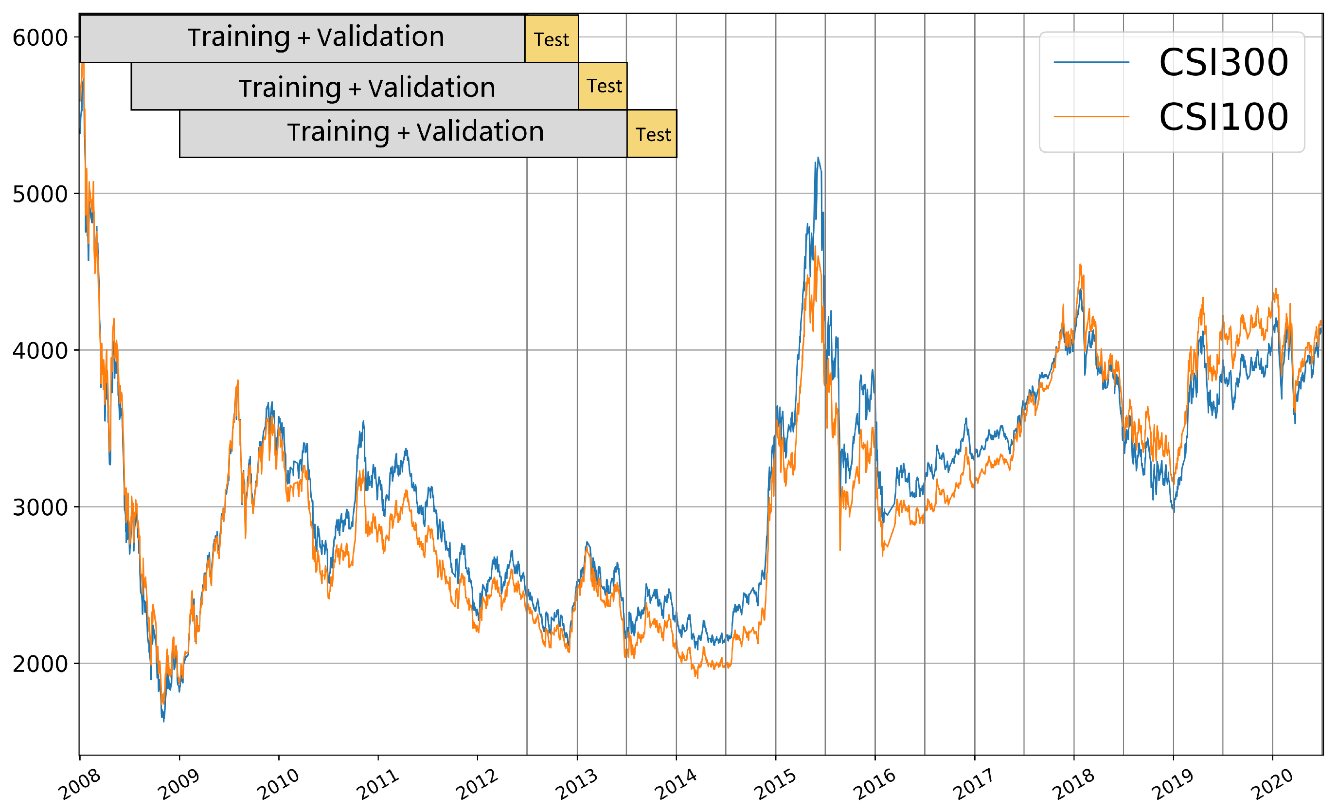
Dataset arrangement. Our dataset contains the historical data for constituent stocks of CSI100 and CSI300 indices from 1 January 2008 to 30 June 2020. Our training approach is conducted in a rolling way. Specifically, we use a 4.5-year dataset to predict the subsequent 0.5-year periods. Thus, the test period is from 1 July 2012 to 30 June 2020 and contains 16 training phases. The training set is also employed to calculate the correlation matrix for the corresponding test set. To prevent overfitting, we randomly sample 15 % of the training set as the validation set at each phase of training.
Figure 3 shows the temporal evolution of the CSI 100 and CSI 300 indices over the period from 1 January 2008 to 30 June 2020, as well as our division of training and testing sets. This time frame encompasses various market styles, including sharp rises, sharp falls, and minor fluctuations. This diversity in market styles can check our model’s performance under different market conditions, ensuring that our model has good generality and robustness.
Evaluation metrics. We first employ three widely used evaluation metrics in the quantitative investment field: the information coefficient (IC), rank IC, and long position cumulative return (CR). Since we cannot short stocks in the Chinese stock market, the prediction of long positions is more vital than short positions, making the evaluation of returns for long positions a more pragmatic indicator.
The information coefficient is the correlation between the security’s actual returns and the investor’s forecasts of returns on those securities [44]. Simulated ICs can help investment managers make determinations for choosing their models. In the actual investment process, stocks with the highest predicted values are selected. Therefore, IC, an indicator that represents the correlation between predicted values and true values, is more useful than MSE, an indicator of absolute error. It might be volatile across time but can still be very useful if carried out carefully [45]. The information coefficient of day t is
I C t = corr ( r t , r ^ t ) .
Here, corr is the Pearson correlation coefficient; r t = ( r 1 t , r 2 t , ) is the real return of stocks of day t, and r ^ t = ( r ^ 1 t , r ^ 2 t , ) is the predicted return of day t. We use the average value of each I C t to represent the I C of the entire period of time.
Similarly, we replace the Pearson correlation coefficient with the Spearman correlation coefficient and obtain R a n k I C of day t.
R a n k I C t = corr ( r a n k r t , r a n k r ^ t ) .
Averaging the daily R a n k I C , we obtain the R a n k I C of the entire test set.
A cumulative return (CR) is the total amount of return generated by an investment within a specified time frame.
CR = current capital initial capital initial capital .
When calculating the long position cumulative return, we simulated buying k stocks with the highest predicted value on each trading day and calculated the cumulative return from the beginning to the end of the test period. We chose k = 50 . We consider excess returns rather than absolute returns. Excess returns, also known as Alpha in the investment field, refer to the returns achieved above and beyond the return of a benchmark index, namely the CSI 100 and CSI 300 indices in this paper. Excess returns are an important metric that helps an investor gauge performance in comparison to other investment alternatives. We use CRexcess in the following results.
CR excess = CR CR benchmark index .
Additionally, given our objective of practical applicability in real-world investment scenarios, we consider the impact of transaction fees, price limits, and suspension of trading. We adopt an initial account capital of 100 million CNY. The commission fee for purchasing stocks is set at 0.05 % , whereas the fee for selling stocks is 0.15 % , with a minimum commission charge of 5 CNY. Stocks are traded in units of 100 shares. The stocks that cannot be traded due to price limits or trading suspensions are excluded while simulating the trading. We use our predictions to build real-world investment portfolios and conduct backtesting, and we compare the annualized excess return (AER), maximum drawdown (MDD), and information ratio (IR) with transaction costs of our backtesting results.
The annualized excess return is the geometric average of an investment’s excess cumulative return in a year.
AER = ( 1 + CR excess ) 365 Days Held 1 .
Here, CRexcess is calculated considering the transaction costs and restrictions mentioned above.
Maximum drawdown is the maximum cumulative loss from a market peak to the following trough [46].
MDD = max { peak value trough value peak value } .
MDD is a metric that tracks the most significant potential percentage decline in the value of a portfolio over a given period. It is a commonly used indicator to measure the risk control ability of a strategy. A lower absolute value of MDD implies a smaller possible maximum loss amplitude.
The information ratio is the average excess return per unit of volatility in excess return [44]. Rooted in the Markowitz mean-variance framework, it aims to provide a single metric that encapsulates the mean-variance characteristics of a portfolio.
IR = E R ¯ t σ ^ ER .
where E R t is the excess return from the benchmark index on day t, and σ ^ ER is the standard deviation of E R t .
Among the above metrics, AER measures the profitability of investment by quantifying the returns generated above a benchmark or risk-free rate. MDD evaluates risk by identifying the largest peak-to-trough decline in the value of an investment, thus providing insights into potential losses and the risk of significant downturns. The information ratio offers a comprehensive metric that balances both returns and risks, as it is calculated by dividing the excess returns by the tracking error, thus indicating how effectively the portfolio generates returns relative to its risk. Collectively, these three metrics provide a multifaceted understanding of an investment portfolio’s performance. By analyzing these indicators in conjunction, one can gain a more nuanced perspective on the portfolio’s profitability and its capacity to manage and mitigate risks effectively.
In order to eliminate the impact of different initializations, we repeat each experiment 10 times and record the average value and standard deviation for all evaluation metrics.

5.4. Predictive Ability of Our Model

Table 1 shows the main results of the five base models with and without our LOG module. All these base models achieve a higher IC, rank IC, and cumulative return with the incorporation of our LOG framework in both the CSI100 and CSI300 markets. In models exclusively focusing on individual stocks, such as MLP, GRU, and LSTM, our module takes into consideration inter-stock correlations, consequently leading to improved performance.
In models such as GAT and Transformer, relationships between stocks have been considered. For example, GAT models rely on the attention mechanism to weigh the importance of neighboring nodes. When the LOG module is integrated, the pre-existing attention mechanism might overshadow the benefits introduced by the correlation weights from the LOG module. This could result in less marginal performance improvements. Similar to GAT, the self-attention mechanism in Transformers may reduce the additional benefit gained from the LOG module as well. However, these models only consider the relationships at the feature level and primarily focus on assessing the similarity between stock features. On this basis, our model directly incorporates the correlation between prices, which is the prediction target. Consequently, our model demonstrates enhanced performance in predictive tasks.

5.5. Backtesting Results

To validate the practical efficacy of our model in real investments, we implemented an investment strategy based on our predictions and conducted backtesting throughout the test period (1 July 2012 to 30 June 2020). The investment strategy is referred to as top-K-strategy. Similar to the calculation of long position return, on each trading day t, we rank all the stocks in the stock pool (CSI100 or CSI300) in descending order of their predicted return values. Then, we select the top k stocks to form the portfolio, wherein an equal allocation of investment capital is made, while any currently held stocks not included in the top k are liquidated. In our experiments, we set k = 50 .
To simulate real-world trading, we assume the buying price to be the closing price of day t + 1 , given that the inclusion of the closing price of day t among the 158 features implies the closure of the stock market on day t, thereby necessitating the purchase of stocks on the next trading day.
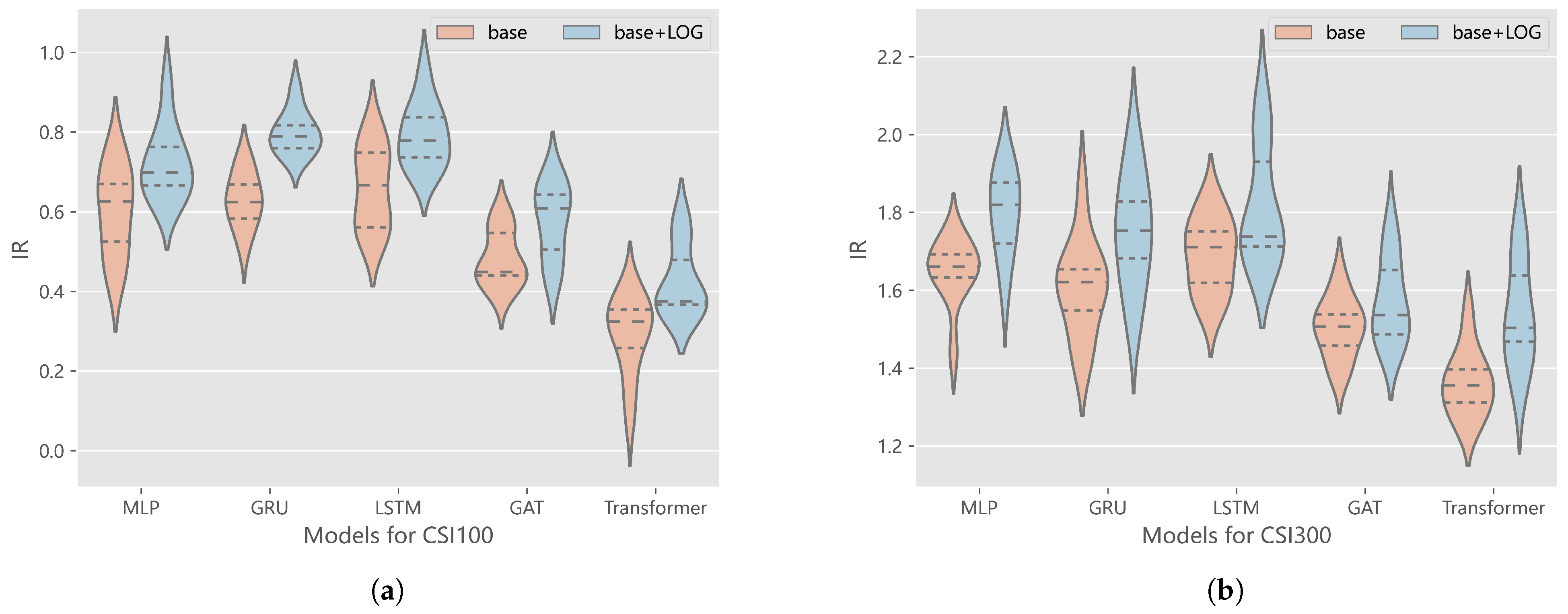
Table 2 shows the results of excess returns with costs, including annualized excess return (AER), maximum drawdown (MDD), and information ratio (IR). Across both the CSI100 and CSI300 markets, the integration of our LOG framework consistently leads to higher annualized excess returns, reduced maximum drawdown, and elevated information ratios for all base models. Figure 4 presents a visualization of the IR results, showing the distribution of IR obtained from the trained models during backtesting. Since we conducted 10 times of experiments for each model, the violin boxplots present outcomes from all the experiments and mark out the 0.25th, 0.5th, and 0.75th quantiles. After adding our LOG, the IR of the backtesting has significantly improved, underscoring the practical value of our method in real-world investment scenarios.

5.6. Statistical Tests on Profitability Improvements

We conducted several statistical tests to demonstrate that the LOG module significantly enhances the profitability of the base models. Let μ 1 be the mean value of profit indicators obtained from the base model, and μ 2 be the mean value of profit indicators obtained from LOG. The null hypothesis is H 0 : μ 1 μ 2 and the alternative hypothesis is H 1 : μ 1 < μ 2 . Our objective is to reject the null hypothesis, thereby substantiating the improvement in profitability introduced by the LOG module. Let x 1 ¯ , x 2 ¯ be the sample average of models without and with LOG, respectively, and s 1 , s 2 be the sample standard deviation of models without and with LOG, respectively. Then, the Welch’s t-test [47] statistic can be formulated as follows:
t w = x 1 ¯ x 2 ¯ s 1 2 n 1 + s 2 2 n 2 .
The degree of freedom is given by
d f = s 1 2 n 1 + s 2 2 n 2 ( s 1 2 / n 1 ) 2 n 1 1 + ( s 2 2 / n 2 ) 2 n 2 1
Welch came up with
t w ˙ t d f
where ˙ means approximately following the distribution, and t d f is the Student’s t distribution with degree of freedom d f .
We take the test on the three profitability metrics, namely CR, AER, and IR, in Table 1 and Table 2. We choose significance level α = 0.1 . The critical value is referred to as t d f , α , where P ( t w t d f , α | H 0 ) = α , and the null hypothesis will be rejected if t w t d f , α .
Table 3, Table 4 and Table 5 show the results of Welch’s t-test on CR, AER, and IR. At the level of significance α = 0.1 , the null hypotheses can be rejected for all cases in CSI100 and for most cases in CSI300, showing that our method improves profitability.

6. Conclusions

In this paper, we propose a LOG framework that characterizes the direct correlation between stock returns to better predict future trends. The integration of our LOG with all base models consistently produced substantial performance improvements. Across the spectrum of evaluation metrics, the incorporation of our framework led to enhanced performance in various evaluation metrics, offering the promise of higher returns coupled with reduced risk in real investment scenarios. These findings underscore the utility and versatility of our approach in the context of stock return prediction, making it a useful addition to the toolkit of practitioners and researchers in the field of financial modeling to build more effective portfolio management strategies. An intriguing future work involves further exploring the applications of graph theory in stock investment, particularly in enhancing the exploration of correlations between individual stocks and devising investment portfolios based on graph-based methodologies.
There are still some limitations to be considered in further studies. First, it is not necessary to use the next two days’ close prices. Various other pricing metrics, such as open price, or VWAP, could be explored to enhance forecasting accuracy and better align with actual trading scenarios. Second, the current experiments are confined to the Chinese financial markets. Extending this research to other financial markets would provide a broader validation of the method’s applicability and robustness. Third, experiments can be conducted on more state-of-the-art models with and without this LOG module to demonstrate its effectiveness. Finally, a potential limitation in calculating correlation coefficients is the dependence on the time scale selected. Different lengths of training set duration introduce variability and uncertainty in the computed correlations, leading to possible pseudo-correlations. Future research could explore how to select time scales to calculate coefficients.

Author Contributions

Conceptualization, W.Z. and B.L.; methodology, W.Z. and B.L.; software, W.Z.; validation, W.Z. and B.L.; formal analysis, W.Z.; investigation, W.Z. and B.L.; resources, W.Z.; data curation, W.Z. and B.L.; writing—original draft preparation, W.Z.; writing—review and editing, B.L.; visualization, W.Z.; supervision, B.L.; project administration, B.L.; funding acquisition, B.L. All authors have read and agreed to the published version of the manuscript.

Funding

This research was funded by the National Natural Science Foundation of China (Grant No. 12371413, No. 22073110) and the Strategic Priority Research Program of Chinese Academy of Sciences (Grant No. XDB0500000).

Institutional Review Board Statement

Not applicable.

Informed Consent Statement

Not applicable.

Data Availability Statement

All data for this research are available at https://github.com/microsoft/qlib (accessed on 1 March 2023).

Acknowledgments

We would like to thank Sheng Gui for his valuable comments and suggestions.

Conflicts of Interest

The authors declare no conflicts of interest.

References

  1. Markowitz, H. Portfolio Selection. J. Financ. 1952, 7, 77–91. [Google Scholar]
  2. Sukcharoen, K.; Leatham, D.J. Dependence and extreme correlation among US industry sectors. Stud. Econ. Financ. 2016, 33, 26–49. [Google Scholar] [CrossRef]
  3. Cao, D.; Long, W.; Yang, W. Sector indices correlation analysis in China’s stock market. Proc. Comput. Sci. 2013, 17, 1241–1249. [Google Scholar] [CrossRef]
  4. Wang, J.J.; Wang, J.Z.; Zhang, Z.G.; Guo, S.P. Stock index forecasting based on a hybrid model. Omega 2012, 40, 758–766. [Google Scholar] [CrossRef]
  5. Kim, R.; So, C.H.; Jeong, M.; Lee, S.; Kim, J.; Kang, J. Hats: A hierarchical graph attention network for stock movement prediction. arXiv 2019, arXiv:1908.07999. [Google Scholar]
  6. Dai, Z.; Zhu, H.; Kang, J. New technical indicators and stock returns predictability. Int. Rev. Econ. Financ. 2021, 71, 127–142. [Google Scholar] [CrossRef]
  7. Liu, M.; Xiao, L.; Jiang, H.; He, Q. CCAT-NET: A Novel Transformer Based Semi-Supervised Framework for COVID-19 Lung Lesion Segmentation. In Proceedings of the 2022 IEEE 19th International Symposium on Biomedical Imaging (ISBI), Kolkata, India, 28–31 March 2022; pp. 1–5. [Google Scholar]
  8. Bhattacharjee, I.; Bhattacharja, P. Stock price prediction: A comparative study between traditional statistical approach and machine learning approach. In Proceedings of the 2019 4th International Conference on Electrical Information and Communication Technology, Khulna, Bangladesh, 20–22 December 2019; pp. 1–6. [Google Scholar]
  9. Ariyo, A.A.; Adewumi, A.O.; Ayo, C.K. Stock price prediction using the ARIMA model. In Proceedings of the 2014 UKSim—AMSS 16th International Conference on Computer Modelling and Simulation, Cambridge, UK, 26–28 March 2014; pp. 106–112. [Google Scholar]
  10. Franses, P.H.; Ghijsels, H. Additive outliers, GARCH and forecasting volatility. Int. J. Forecast. 1999, 15, 1–9. [Google Scholar] [CrossRef]
  11. Nair, B.B.; Mohandas, V.; Sakthivel, N. A decision tree-rough set hybrid system for stock market trend prediction. Int. J. Comput. Appl. 2010, 6, 1–6. [Google Scholar] [CrossRef]
  12. Wang, J.L.; Chan, S.H. Stock market trading rule discovery using two-layer bias decision tree. Expert Syst. Appl. 2006, 30, 605–611. [Google Scholar] [CrossRef]
  13. Grigoryan, H. A Stock Market Prediction Method Based on Support Vector Machines (SVM) and Independent Component Analysis (ICA). Database Syst. J. 2016, 7, 12–21. [Google Scholar]
  14. Tay, F.E.; Cao, L. Application of support vector machines in financial time series forecasting. Omega 2001, 29, 309–317. [Google Scholar] [CrossRef]
  15. Ho, T.K.; Hull, J.J.; Srihari, S.N. Decision combination in multiple classifier systems. IEEE Trans. Pattern Anal. Mach. Intell. 1994, 16, 66–75. [Google Scholar]
  16. Khaidem, L.; Saha, S.; Dey, S.R. Predicting the direction of stock market prices using random forest. arXiv 2016, arXiv:1605.00003. [Google Scholar]
  17. Tsai, C.F.; Lin, Y.C.; Yen, D.C.; Chen, Y.M. Predicting stock returns by classifier ensembles. Appl. Soft Comput. 2011, 11, 2452–2459. [Google Scholar] [CrossRef]
  18. Pan, H.; Tilakaratne, C.; Yearwood, J. Predicting the Australian stock market index using neural networks exploiting dynamical swings and intermarket influences. In Proceedings of the AI 2003: Advances in Artificial Intelligence, Perth, Australia, 3–5 December 2003; pp. 327–338. [Google Scholar]
  19. Situngkir, H.; Surya, Y. Neural network revisited: Perception on modified Poincare map of financial time-series data. Phys. A Stat. Mech. Its Appl. 2004, 344, 100–103. [Google Scholar] [CrossRef]
  20. Turchenko, V.; Beraldi, P.; De Simone, F.; Grandinetti, L. Short-term stock price prediction using MLP in moving simulation mode. In Proceedings of the 6th IEEE International Conference on Intelligent Data Acquisition and Advanced Computing Systems, Prague, Czech Republic, 15–17 September 2011; Volume 2, pp. 666–671. [Google Scholar]
  21. Chen, K.; Zhou, Y.; Dai, F. A LSTM-based method for stock returns prediction: A case study of China stock market. In Proceedings of the 2015 IEEE International Conference on Big Data, Santa Clara, CA, USA, 29 October–1 November 2015; pp. 2823–2824. [Google Scholar]
  22. Nelson, D.M.; Pereira, A.C.; De Oliveira, R.A. Stock market’s price movement prediction with LSTM neural networks. In Proceedings of the 2017 International Joint Conference on Neural Networks, Anchorage, AL, USA, 14–19 May 2017; pp. 1419–1426. [Google Scholar]
  23. Roondiwala, M.; Patel, H.; Varma, S. Predicting stock prices using LSTM. Int. J. Sci. Res. 2017, 6, 1754–1756. [Google Scholar]
  24. Qu, G.; Hu, W.; Xiao, L.; Wang, J.; Bai, Y.; Patel, B.; Zhang, K.; Wang, Y.P. Brain Functional Connectivity Analysis via Graphical Deep Learning. IEEE Trans. Biomed. Eng. 2022, 69, 1696–1706. [Google Scholar] [CrossRef] [PubMed]
  25. Xu, W.; Liu, W.; Wang, L.; Xia, Y.; Bian, J.; Yin, J.; Liu, T.Y. Hist: A graph-based framework for stock trend forecasting via mining concept-oriented shared information. arXiv 2021, arXiv:2110.13716. [Google Scholar]
  26. Li, W.; Bao, R.; Harimoto, K.; Chen, D.; Xu, J.; Su, Q. Modeling the stock relation with graph network for overnight stock movement prediction. In Proceedings of the 29th International Joint Conference on Artificial Intelligence, Yokohama, Japan, 11–17 July 2020; pp. 4541–4547. [Google Scholar]
  27. Long, J.; Chen, Z.; He, W.; Wu, T.; Ren, J. An integrated framework of deep learning and knowledge graph for prediction of stock price trend: An application in Chinese stock exchange market. Appl. Soft Comput. 2020, 91, 106205. [Google Scholar] [CrossRef]
  28. Wu, J.; Xu, K.; Chen, X.; Li, S.; Zhao, J. Price graphs: Utilizing the structural information of financial time series for stock prediction. Inf. Sci. 2022, 588, 405–424. [Google Scholar] [CrossRef]
  29. Ding, Q.; Wu, S.; Sun, H.; Guo, J.; Guo, J. Hierarchical Multi-Scale Gaussian Transformer for Stock Movement Prediction. In Proceedings of the 29th International Joint Conference on Artificial Intelligence, Yokohama, Japan, 11–17 July 2020; pp. 4640–4646. [Google Scholar]
  30. Zhong, X.; Enke, D. Forecasting daily stock market return using dimensionality reduction. Expert Syst. Appl. 2017, 67, 126–139. [Google Scholar] [CrossRef]
  31. Zhong, X.; Enke, D. Predicting the daily return direction of the stock market using hybrid machine learning algorithms. Financ. Innov. 2019, 5, 24. [Google Scholar] [CrossRef]
  32. Singh, H.; Sharma, R. Role of adjacency matrix & adjacency list in graph theory. Int. J. Comput. Technol. 2012, 3, 179–183. [Google Scholar]
  33. Tumminello, M.; Aste, T.; Di Matteo, T.; Mantegna, R.N. A tool for filtering information in complex systems. Proc. Natl. Acad. Sci. USA 2005, 102, 10421–10426. [Google Scholar] [CrossRef] [PubMed]
  34. Dees, B.S.; Stanković, L.; Constantinides, A.G.; Mandic, D.P. Portfolio cuts: A graph-theoretic framework to diversification. In Proceedings of the ICASSP 2020—2020 IEEE International Conference on Acoustics, Speech and Signal Processing (ICASSP), Virtual, 4–9 May 2020; pp. 8454–8458. [Google Scholar]
  35. Mantegna, R.N. Hierarchical structure in financial markets. Eur. Phys. J. Condens. Matter Complex Syst. 1999, 11, 193–197. [Google Scholar] [CrossRef]
  36. Engle, R. Dynamic Conditional Correlation. J. Bus. Econ. Stat. 2002, 20, 339–350. [Google Scholar] [CrossRef]
  37. Karanasos, M.; Paraskevopoulos, A.G.; Menla Ali, F.; Karoglou, M.; Yfanti, S. Modelling stock volatilities during financial crises: A time varying coefficient approach. J. Empir. Financ. 2014, 29, 113–128. [Google Scholar] [CrossRef]
  38. Yang, X.; Liu, W.; Zhou, D.; Bian, J.; Liu, T.Y. Qlib: An ai-oriented quantitative investment platform. arXiv 2020, arXiv:2009.11189. [Google Scholar]
  39. Chung, J.; Gulcehre, C.; Cho, K.; Bengio, Y. Empirical evaluation of gated recurrent neural networks on sequence modeling. arXiv 2014, arXiv:1412.3555. [Google Scholar]
  40. Hochreiter, S.; Schmidhuber, J. Long short-term memory. Neural Comput. 1997, 9, 1735–1780. [Google Scholar] [CrossRef]
  41. Veličković, P.; Cucurull, G.; Casanova, A.; Romero, A.; Lio, P.; Bengio, Y. Graph attention networks. arXiv 2017, arXiv:1710.10903. [Google Scholar]
  42. Vaswani, A.; Shazeer, N.; Parmar, N.; Uszkoreit, J.; Jones, L.; Gomez, A.N.; Kaiser, Ł.; Polosukhin, I. Attention is all you need. In Advances in Neural Information Processing Systems; Neural Information Processing Systems Foundation, Inc. (NeurIPS): La Jolla, CA, USA, 2017; Volume 30. [Google Scholar]
  43. Wang, C.; Chen, Y.; Zhang, S.; Zhang, Q. Stock market index prediction using deep Transformer model. Expert Syst. Appl. 2022, 208, 118128. [Google Scholar] [CrossRef]
  44. Goodwin, T.H. The Information Ratio. Financ. Anal. J. 1998, 54, 34–43. [Google Scholar] [CrossRef]
  45. Zhang, F.; Guo, R.; Cao, H. Information Coefficient as a Performance Measure of Stock Selection Models. arXiv 2020, arXiv:2010.08601. [Google Scholar]
  46. Magdon-Ismail, M.; Atiya, A.F. Maximum drawdown. Risk Mag. 2004, 17, 99–102. [Google Scholar]
  47. Lu, Z.; Yuan, K.H. Welch’s t Test; Sage: Thousand Oaks, CA, USA, 2010; pp. 1620–1623. [Google Scholar]
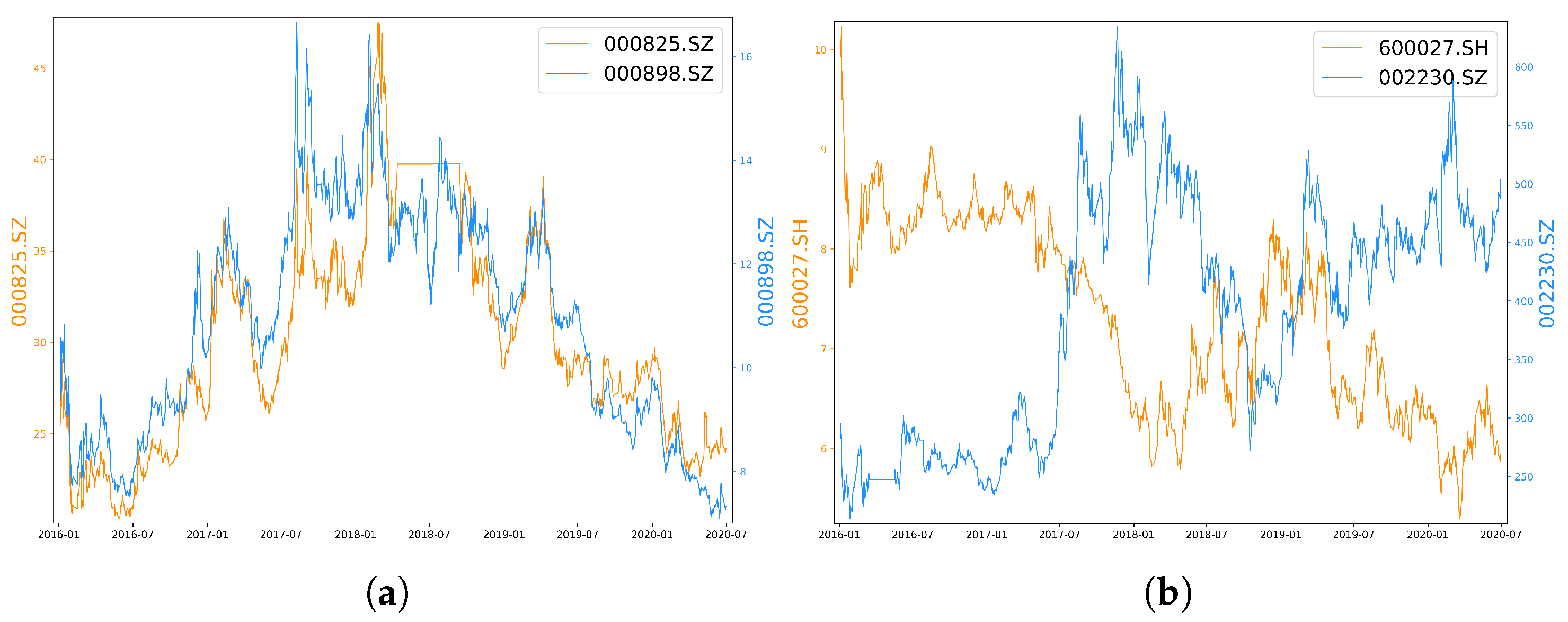
Figure 1. Correlations in stock prices (both positive and negative correlations). (a) Trend chart of 000825.SZ and 000898.SZ (unit: CNY). (b) Trend chart of 600027.SH and 002230.SZ (unit: CNY).
Bdcc 08 00056 g001
Figure 2. The framework of our LOG.
Bdcc 08 00056 g002
Figure 3. The indices tendency (unit: point) and dataset arrangement.
Bdcc 08 00056 g003
Figure 4. Results of IR and quantiles (0.25/0.5/0.75 quantiles). (a) Distribution of IR for CSI100. (b) Distribution of IR for CSI300.
Bdcc 08 00056 g004
Table 1. Predictive ability (and its standard deviation) on CSI100 and CSI300.
MethodsCSI100CSI300
ICRank ICCRICRank ICCR
MLP0.0649
(1.60 × 10 3 )
0.0628
(1.69 × 10 3 )
0.9836
(1.05 × 10 1 )
0.0747
(1.22 × 10 3 )
0.0717
(1.23 × 10 3 )
3.6233
(2.75 × 10 1 )
MLP + LOG0.0666
(8.96 × 10 4 )
0.0645
(1.26 × 10 3 )
1.1015
(9.14 × 10 2 )
0.0752
(8.70 × 10 4 )
0.0727
(8.82 × 10 4 )
3.9937
(2.94 × 10 1 )
GRU0.0653
(8.31 × 10 4 )
0.0625
(8.74 × 10 4 )
1.0086
(6.80 × 10 2 )
0.0761
(8.58 × 10 4 )
0.0733
(9.16 × 10 4 )
3.4192
(2.98 × 10 1 )
GRU + LOG0.0680
(1.23 × 10 3 )
0.0655
(1.47 × 10 3 )
1.1753
(5.92 × 10 2 )
0.0770
(1.27 × 10 3 )
0.0740
(1.15 × 10 3 )
3.7135
(3.80 × 10 1 )
LSTM0.0654
(1.75 × 10 3 )
0.0632
(1.69 × 10 3 )
1.0387
(9.44 × 10 2 )
0.0735
(1.16 × 10 3 )
0.0706
(1.14 × 10 3 )
3.6282
(2.40 × 10 1 )
LSTM + LOG0.0666
(1.58 × 10 3 )
0.0641
(1.65 × 10 3 )
1.1634
(8.00 × 10 2 )
0.0737
(1.06 × 10 3 )
0.0710
(9.41 × 10 4 )
3.8031
(4.08 × 10 1 )
GAT0.0594
(2.64 × 10 3 )
0.0573
(2.22 × 10 3 )
0.8648
(6.03 × 10 2 )
0.0713
(1.36 × 10 3 )
0.0690
(1.16 × 10 3 )
3.1322
(1.97 × 10 1 )
GAT + LOG0.0615
(2.20 × 10 3 )
0.0592
(2.33 × 10 3 )
0.9552
(8.58 × 10 2 )
0.0716
(1.74 × 10 3 )
0.0693
(1.82 × 10 3 )
3.2590
(2.60 × 10 1 )
Transformer0.0561
(1.76 × 10 3 )
0.0555
(1.90 × 10 3 )
0.7026
(7.95 × 10 2 )
0.0665
(1.74 × 10 3 )
0.0653
(1.67 × 10 3 )
2.9362
(2.59 × 10 1 )
Transformer + LOG0.0573
(2.22 × 10 3 )
0.0574
(1.69 × 10 3 )
0.8176
(7.75 × 10 2 )
0.0700
(1.56 × 10 3 )
0.0683
(1.45 × 10 3 )
3.1703
(3.14 × 10 1 )
Table 2. Backtesting results (and their standard deviation) on CSI100 and CSI300.
MethodsCSI100CSI300
AERMDDIRAERMDDIR
MLP0.0412
(7.24 × 10 3 )
−0.1371
(1.22 × 10 2 )
0.6013
(1.05 × 10 1 )
0.1624
(9.34 × 10 3 )
−0.1800
(1.86 × 10 2 )
1.6493
(7.92 × 10 2 )
MLP + LOG0.0491
(5.88 × 10 3 )
−0.1299
(1.03 × 10 2 )
0.7217
(8.71 × 10 2 )
0.1741
(9.10 × 10 3 )
−0.1719
(7.16 × 10 3 )
1.8003
(1.04 × 10 1 )
GRU0.0432
(4.62 × 10 3 )
−0.1284
(1.33 × 10 2 )
0.6299
(6.60 × 10 2 )
0.1556
(1.01 × 10 2 )
−0.1956
(1.82 × 10 2 )
1.6079
(1.16 × 10 1 )
GRU + LOG0.0542
(3.67 × 10 3 )
−0.1212
(8.43 × 10 3 )
0.7985
(5.15 × 10 2 )
0.1652
(1.21 × 10 2 )
−0.1771
(1.30 × 10 2 )
1.7529
(1.39 × 10 1 )
LSTM0.0455
(6.20 × 10 3 )
−0.1246
(7.48 × 10 3 )
0.6606
(9.62 × 10 2 )
0.1628
(7.89 × 10 3 )
−0.1776
(1.44 × 10 2 )
1.6899
(8.95 × 10 2 )
LSTM + LOG0.0540
(4.98 × 10 3 )
−0.1257
(6.62 × 10 3 )
0.7923
(7.70 × 10 2 )
0.1681
(1.27 × 10 2 )
−0.1750
(2.40 × 10 2 )
1.8163
(1.43 × 10 1 )
GAT0.0334
(4.28 × 10 3 )
−0.1344
(1.68 × 10 2 )
0.4820
(6.55 × 10 2 )
0.1457
(7.06 × 10 3 )
−0.1815
(1.08 × 10 2 )
1.5031
(7.30 × 10 2 )
GAT + LOG0.0398
(5.95 × 10 3 )
−0.1308
(1.31 × 10 2 )
0.5763
(8.76 × 10 2 )
0.1501
(9.02 × 10 3 )
−0.1794
(1.75 × 10 2 )
1.5731
(1.03 × 10 1 )
Transformer0.0203
(6.39 × 10 3 )
−0.1469
(2.47 × 10 2 )
0.2910
(9.25 × 10 2 )
0.1380
(9.51 × 10 3 )
−0.1870
(1.28 × 10 2 )
1.3612
(8.10 × 10 2 )
Transformer + LOG0.0292
(5.64 × 10 3 )
−0.1342
(1.22 × 10 2 )
0.4251
(8.35 × 10 2 )
0.1466
(1.12 × 10 2 )
−0.1741
(2.42 × 10 2 )
1.5373
(1.29 × 10 1 )
Table 3. Welch’s t-test for cumulative return (CR).
MethodsCSI100CSI300
twdftdf,αtwdftdf,α
MLP−2.5418−1.330−2.7618−1.330
GRU−5.5518−1.330−1.8217−1.333
LSTM−3.0318−1.330−1.1318−1.330
GAT−2.5916−1.337−1.1818−1.330
Transformer−3.1118−1.330−1.7217−1.333
Table 4. Welch’s t-test for annualized excess return (AER).
MethodsCSI100CSI300
twdftdf,αtwdftdf,α
MLP−2.5517−1.333−2.6818−1.330
GRU−5.5917−1.333−1.8317−1.333
LSTM−3.2117−1.333−1.1618−1.330
GAT−2.6316−1.337−1.2217−1.333
Transformer−3.1118−1.330−1.7418−1.330
Table 5. Welch’s t-test for information ratio (IR).
MethodsCSI100CSI300
twdftdf,αtwdftdf,α
MLP−2.6417−1.333−3.4717−1.333
GRU−6.0417−1.333−2.3917−1.333
LSTM−3.2117−1.333−2.2515−1.341
GAT−2.5917−1.333−1.6616−1.337
Transformer−3.2318−1.330−3.4715−1.341
Disclaimer/Publisher’s Note: The statements, opinions and data contained in all publications are solely those of the individual author(s) and contributor(s) and not of MDPI and/or the editor(s). MDPI and/or the editor(s) disclaim responsibility for any injury to people or property resulting from any ideas, methods, instructions or products referred to in the content.