Abstract
This research aims at applying the Artificial Organic Network (AON), a nature-inspired, supervised, metaheuristic machine learning framework, to develop a new algorithm based on this machine learning class. The focus of the new algorithm is to model and predict stock markets based on the Index Tracking Problem (ITP). In this work, we present a new algorithm, based on the AON framework, that we call Artificial Halocarbon Compounds, or the AHC algorithm for short. In this study, we compare the AHC algorithm against genetic algorithms (GAs), by forecasting eight stock market indices. Additionally, we performed a cross-reference comparison against results regarding the forecast of other stock market indices based on state-of-the-art machine learning methods. The efficacy of the AHC model is evaluated by modeling each index, producing highly promising results. For instance, in the case of the IPC Mexico index, the R-square is 0.9806, with a mean relative error of . Several new features characterize our new model, mainly adaptability, dynamism and topology reconfiguration. This model can be applied to systems requiring simulation analysis using time series data, providing a versatile solution to complex problems like financial forecasting.
1. Introduction
The handling of risk and uncertainty across various financial domains has prompted the development of diverse models and methodologies. As exposed by Elliot and Timmermann [1], asset allocation requires real-time stock return forecasts, and improved predictions contribute to enhanced investment performance. Consequently, the ability to forecast returns holds crucial implications for testing market efficiency and developing more realistic asset pricing models that better reflect the available data. Furthermore, Elliot and Timmermann [1] state that stock returns inherently contain a sizable unpredictable component, so the best forecasting models can only explain a relatively small part of stock returns.
In this respect, we propose a new algorithm, called Artificial Halocarbon Compounds (AHC), or the AHC algorithm for short, to tackle the Index Tracking Problem (ITP). The efficacy is evaluated by forecasting eight stock market indices. The outcomes obtained using the AHC model, as an alternative topology rooted in the Artificial Organic Network (AON), are compared to the results obtained using genetic algorithms (GAs) as a benchmark. Additionally, we performed a cross-reference comparison against results regarding the forecast of other stock market indices based on state-of-the-art machine learning methods. The efficacy of the AHC model is evaluated by modeling each index, producing highly promising results. For instance, in the case of the IPC Mexico index, the R-square is 0.9806, with a mean relative error of . From this perspective, the objective is aligned with the aim previously outlined in [2], centered on crafting a novel, efficient algorithm based on the AON framework that is capable of producing short-term forecasts for market trends.
The AON is a supervised machine learning framework. It comprises a collection of graphs constructed using heuristic rules to assemble organic compounds, enabling the modeling of systems in a gray-box manner. Each graph within this framework represents a molecule, essentially acting as information packages that offer partial insights into understanding the behavior of the system. The rationale behind considering GAs as a benchmark is that, although GAs are not traditionally categorized as a distinct subdivision of machine learning and are often associated with stochastic optimization, they have been extensively applied in financial forecasting tasks [3,4]. Moreover, as illustrated in Section 2.2.1, Artificial Hydrocarbon Networks, or AHN, the formally defined topology of the AON, has been subject to comparison with various other methods. Hence, building upon the previous fact, and given that the GA has been used in financial forecasting with success, it was selected as the benchmark for comparison.
The rest of the article is structured as follows. In Section 2, we present a literature review concerning stock mark index prediction using machine learning methods. Additionally, the main concepts of the AHC algorithm are illustrated, as well as some details about the machine learning class by which it was inspired, the AON framework, including some previously reported implementations. This section also provides some main concepts about GAs. Next, in Section 3, we give details about the data used and how data were preprocessed. We also describe the methodology followed to perform the experiments. Afterward, Section 4 explains how the methods were implemented describing the parameter tuning process. Section 5 presents the results of each method as well as a cross-reference comparison. Finally, Section 6 gives the conclusions of the study and presents insights into possible future investigation lines.
2. Background
In this section, a contextual theoretical framework is presented. Specifically, Section 2.1 provides a literature review. Further, Section 2.2 explains the Artificial Halocarbon Compounds method as a novel topology based on AON principles. This section also shares a comparison of Artificial Hydrocarbon Networks (the initially defined AON topology), to other existing methods. Later, Section 2.3 provides a brief overview of genetic algorithms.
2.1. Literature Review
Several works can be found across the literature explaining the complexity of forecasting stock market indices, due to their noisy, unpredictable, nonlinear dynamics as main characteristics of their behavior, and considering the application of different machine learning techniques as state-of-the-art predicting tools. In this respect, Ayyıldız [5] offers a literature review of machine learning algorithms applied to the prediction of stock market indices. Saboor et al. [6] delivered the forecast of the KSE 100 (Karachi Stock Exchange), the DSE 30 (Dhaka Stock Exchange) and the BSE Sensex (Bombay Stock Exchange) using methods such as Support Vector Regression (SVR), Random Forest Regression (RF) and Long Short-Term Memory (LSTM). In contrast, Aliyev et al. [7], offer the prediction of the RTS Index (Russian Stock Exchange), applying an ARIMA-GARCH model and an LSTM model. Ding et al. [8], performed similar work while producing the projection of the SSE (Shanghai Stock Exchange) using ARIMA and LSTM models. In their work, Haryono et al. [9] present the forecast of the IDX (Indonesia Stock Exchange) by applying different combinations of architectures using Convolutional Neural Networks (CNNs), Gated Recurrent Units (GRUs) and LSTM, implemented through TensorFlow (TF). Similarly to Haryono, Pokhrel et al. [10] performed the forecast of the NEPSE (Nepal Stock Exchange), employing CNN, GRU and LSTM architectures. Further, Singh [11] forecast the Nifty 50 (Indian Stock Market Index) using eight machine learning models, including Adaptive Boost (AdaBoost), k-Nearest Neighbors (KNN) and Artificial Neural Networks (ANNs), among others. As a final example, Harahap et al. [12] present the usage of Deep Neural Networks (DNNs), Back Propagation Neural Networks (BPNNs) and SVR techniques for the forecast of the N225. A summary and a brief discussion of the results presented in this section are given in Section 5.3.
2.2. Artificial Halocarbon Compounds
Artificial Halocarbon Compounds (AHC) or the AHC algorithm, as a learning method, is a new topology based on the AON framework inspired by chemical halocarbon compounds. The AON is a supervised metaheuristic bio-inspired machine learning class introduced by Ponce et al. [13,14]. As defined, the AON is based on heuristic rules inspired by chemistry to create a set of graphs that represent molecules with atoms as vertices and chemical bonds as edges; the molecules interact through chemical balance to form a mixture of compounds. In this regard, the AON builds organic compounds and defines their interactions; the structure of molecules produced can be seen as packages of information that allow us to model nonlinear systems.
As stated by Ponce et al. [13,14], the implementation of the AON requires the utilization of a functional group. These functional groups act as the kinds of molecules that dictate the topological configuration of the AON during its application. Consequently, the AON has been instantiated using a specific existing topology known as Artificial Hydrocarbon Networks (AHN). Therefore, the AHN model is the initial and sole formally defined topology for the AON thus far. The AHN algorithm is conceptualized as biochemically inspired by the formation of chemical hydrocarbon compounds. It was designed to optimize a cost–energy function, employing two mechanisms for the creation of organic compounds. These mechanisms aim to generate an efficient number of molecules to construct the desired structures. These tools are as follows:
- Least-squares regression (LSR) to define the structure of each molecule.
- Gradient descent (GD) to optimize the position and number of molecules in the feature space.
While AHN has demonstrated enhanced predictive power and interpretability when compared to other prominent machine learning models like neural networks and random forests, it does have certain limitations. As explained in [15], big data is primarily characterized by the volume of information to be processed, the velocity of data generation and the diversity of data types involved. Existing machine learning algorithms must be adapted to harness the advantages of big data and efficiently handle larger amounts of information. In this context, AHN faces a drawback as it is notably time-consuming and struggles to cope with big data requirements. The model employs gradient descent (GD), which, due to its inherent complexity, poses challenges to the scalability of the AHN model.
2.2.1. Formerly Reported Comparison and Implementations of AHN
Previously, Ponce [13,14] delineated a comprehensive comparison between the AHN algorithm and various conventional machine learning and optimization methods. This evaluation encompassed considerations of computational complexity, attributes of learning algorithms and features of the constructed models, alongside the types of problems addressed. In this regard, Table 1 illustrates part of the comparison performed by Ponce, showing the computational complexity of learning algorithms and some of their characteristics, such as being supervised or unsupervised, among other attributes. Additionally, Table 1 provides insights into some of the specific problem types that each algorithm can effectively tackle, including approximation or prediction, classification and optimization. In this regard, the AHN algorithm is noteworthy for constructing a continuous, nonlinear and static model within a given system.

Table 1.
Some identified attributes for certain learning algorithms compared by Ponce [13,14].
Numerous applications of the AHN algorithm across diverse fields have been documented since its proposition by Ponce [13]. Some of the reported applications are as follows:
- Online sales prediction: The AHN algorithm has been applied in forecasting online retail sales, employing a simple AHN topology featuring a linear and saturated compound. The implementation involved a comparative analysis with other well-established learning methods, including cubic splines (CSs), model trees (MTs), random forest (RF), linear regression (LR), Bayesian regularized neural networks (BNs), support vector machines with a radial basis function kernel (SVM), among others. Performance evaluation in the experiments was conducted based on the accuracy of the models, measured by the root-mean squared error (RMSE) metric. Notably, the results revealed that AHN outperformed the other models, demonstrating superior performance in this context [16].
- Forecast of exchange rate currencies: the effectiveness of the AHN model in generating forecasts for the exchange rates of BRICS currencies to USD was assessed. Specifically, the work focused on the exchange rate of the Brazilian Real to USD (BRL/USD). Following the execution of experiments, the model yielded a favorable chart behavior, accompanied by an error rate of 0.0102 [17].
- The AHN algorithm was employed in an intelligent diagnosis system using a double-optimized Artificial Hydrocarbon Network to identify mechanical faults in the In-Wheel Motor (IWM). The implementation aimed to validate enhanced performance across multiple rotating speeds and load conditions for the IWM. Comparative analysis was conducted against other methods, including support vector machines (SVMs), a particle swarm optimization-based SVM (PSO-SVM), among others. The double-optimized AHN method exhibited superior performance, achieving a diagnosis accuracy surpassing 80% [18].
These instances represent just a few examples of the diverse applications where AHN has demonstrated favorable outcomes. For readers seeking more in-depth information on specific cases mentioned here or desiring a broader understanding of the varied purposes for which AHN has been employed, it is recommended to explore the lectures by Ponce et al. referenced in this work [13,14,15,16,17,18,19,20,21,22].
2.2.2. Artificial Halocarbon Compounds Approach
Artificial Halocarbon Compounds (AHC) or the AHC algorithm for short, represents a novel supervised machine learning algorithm rooted in the AON framework, drawing inspiration from chemical halocarbon compounds. As a distinctive AON arrangement, its primary emphasis is on forgoing the gradient descent (GD) mechanism to optimize the position and/or number of molecules. This strategic choice aims to mitigate time consumption during the creation of an AON structure. In this hybrid approach, the feature space undergoes segmentation, or clustering, utilizing K-means based on the required number of molecules. This segmentation determines the position of each molecule. Consequently, with each iteration, the data are segmented as many times as the specified number of molecules to be created. Subsequently, the structure of each molecule is computed for the corresponding segment. Rather than employing a conventional least-squares regression (LSR) method to directly define the structure of each molecule, a dynamic topology is introduced as a significant feature shaping the new AON arrangement.
In this context, the dynamic topology provides flexibility by allowing a broader range of options to construct organic structures for a compound. This selection is based on the cost–energy function, ensuring the overall low error of the produced models. These dynamic options involve decisions such as substituting the type of curve or choosing among different fitting methods, including the multiple nonlinear regressive (MNLR) model [2], among others. This involves replacing the method used to characterize each molecule. These replacements are analyzed during the computation of the algorithm, simulating a chemical reaction. At the end of the reaction, the arrangement with the most favorable final substitution from the compared structures is presented.
2.2.3. AHC Algorithm Implementation
The AHC algorithm is implemented through the routine presented in Algorithm 1. In addition, Figure 1 shows a flowchart with the phases of the AHC algorithm. The corresponding input variables that the algorithm receives to produce a model are (a) the dataset (denoted as the system), (b) the maximum number of molecules allowed for the compound structure, (c) the tolerance value for the error and (d) the regularization factor considered along the computations. The maximum number of molecules and the tolerance value are used as criteria for the stopping condition of the algorithm; in this sense, the routine stops once one of the two is met. The outputs of the algorithm are (a) the structure of the compound and (b) the type of halogenation (the chemical reaction) produced in each molecule. The coefficients of the model are held inside the compound structure. The entropy-rule considered in the algorithm is a characteristic of the AHC model, whose objective is to maintain the lowest entropy (level of energy) of the model system, taking into account the output error.
| Algorithm 1 AHC Algorithm (): Implementation of the Artificial Halocarbon Compounds using the AHC algorithm. |
Input: the system , the maximum number of molecules , the tolerance value and the regularization factor . Output: the structure of the compound C and the type of halogenation for each molecule in C. The coefficients are included within the structure C.
|
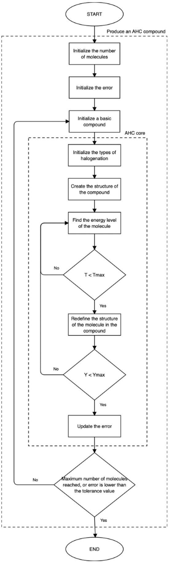
Figure 1.
Flowchart illustrating the phases of the AHC algorithm to produce a compound to model a system.
2.3. Genetic Algorithms
Genetic algorithms (GAs), as explained in [3,4], are metaheuristic, nature-inspired algorithms that are classified under evolutionary algorithms (EAs), that work by imitating the evolutionary process of natural selection and genetics. In contrast, as Ponce [23] recalls, the GA functions as a mathematical object that transforms a set of mathematical entities over time through a series of genetic operations, notably including sexual recombination. These operations adhere to patterned procedures based on the Darwinian principle of reproduction and the survival of the fittest. Typically, each mathematical object takes the form of a string of characters (letters or numbers) of a fixed length, resembling chains of chromosomes. These entities are associated with a defined fitness function that gauges their aptitude. To elaborate, a genetic algorithm operates within a given population, subjecting it to an evolutionary process to generate new generations. Usually, the algorithm concludes when most individuals in a population become nearly identical or when a predefined termination criterion is met; while GAs are not typically considered a specific subdivision of machine learning (ML), they can be utilized in various aspects of ML. They are particularly used in stochastic optimization and search problems and have been widely used in financial forecasting tasks.
3. Methodology
Distinct experiments have been conducted to validate the efficacy of the AHC algorithm, put forth as a suggested supervised machine learning algorithm, and can successfully conduct short-term forecasts of market price trends, as initially specified in [2]. In this context, Section 3.1 details the utilized data and outlines the preprocessing steps undertaken for the experiments. Subsequently, Section 4 provides insight into the selection of the parameters for the implementation of the AHC algorithm for forecasting eight stock market indices, as well as the parameters used in GA models for the same forecasting purpose.
3.1. Data
For these experiments, we used the existing data of the closing price of eight indices, from six countries. The indices are IPC, S&P 500, DAX, DJIA, FTSE, N225, NDX and CAC; Table 2 shows some descriptive statistics for the closing price of the stock market indices used in this research.
Table 2.
Descriptive statistics of the closing price of the corresponding stock market indices.
For each index model, the variables included in the dataset are the daily reported stock market index closing price, the quarterly reported gross domestic product (GDP), the daily reported foreign exchange rate (FX), the monthly reported consumer price index (CPI), the monthly risk-free rate (RFR), the monthly unemployment rate (UR), the monthly reported current account to GDP rate (BOP) and the monthly reported investment rate (GFCF). The time period is from the 1st of June 2006 to the 31st of May 2023. We chose this time period to ensure that at least one short economic cycle was used for the analysis and prediction [2]. The indices and the FX data were sourced from Yahoo Finance, and the rest of the variables were retrieved from the OECD. The data are available at [24] and were preprocessed as follows:
- 1
- For each input, we applied an approximation using least-squares polynomial (LSP) regression; in this regard, the macroeconomic variables (MEVs) are treated as “continuous signals” instead of discrete information.
- 2
- The data were standardized by removing the mean so it could be scaled.
- 3
- We used principal component analysis (PCA) to reduce the dimensionality of the data; it was carried out by considering three principal components (PCs).
It is crucial to emphasize that, although eight may be considered a relatively small number of features, the utilization of PCA plays an essential role in the implementation of AHC; this arises from the fact that the computational complexity of the original AHN topology was dependent on the number of features. The models are evaluated by applying an out-of-sample forecast. The criteria for employing an out-of-sample forecast instead of a one-day-ahead forecast (despite the latter method being a more common forecast practice) pertain to the progress achieved for the ongoing investigation at the moment these results were collected. Out-of-sample forecasting refers to the practice of testing the performance of a financial model or forecasting method on data that were not used in the model’s development. Essentially, the idea is to evaluate how well a model generalizes to new, unseen data. This is a crucial step in assessing the reliability and effectiveness of a forecasting model, as it provides insights into how well the model is likely to perform in real-world scenarios. In contrast, a one-day-ahead forecast involves predicting the financial market’s conditions or the price of an asset for the next trading day. This short-term forecast is used by investors and traders to make informed decisions on buying or selling securities based on expected market movements within the next day.
To avoid overfitting, besides the consideration that the AHC algorithm uses the parameter as a regularization factor, the data were preprocessed accordingly as mentioned above. The procedure to fine-tune the value is explained in Section 4.1. In addition, the data were split in two: the initial 85% for training and the remaining 15% for testing. This split size was chosen because, as outlined in Section 5.1, we conducted a comparison of the performance of the AHC algorithm vs. the GA. In this regard, after conducting parameter tuning for the GA, that included different values of the split size, the best results for the GA were obtained using a testing size of 15%.
3.2. Forecast of the Stock Market Indices
To produce the forecast of the stock market indices, first, all data were preprocessed as described in Section 3.1; subsequently, the dataset was passed to each algorithm. The training parameters for the AHC algorithm and GA methods were established by carrying out a grid search, explained with further detail in Section 4. Once we established the training parameters, the models were fitted using the training set. Afterward, the models were used to conduct a forecast with the testing sets. The performance of each method is compared in Section 5; the section also contains a comparison of the AHC algorithm against some of the results found across the literature review. The described methodology is illustrated in Figure 2.

Figure 2.
Methodology to compare the results of the forecast of stock market indices with different methods.
For the interested reader, the code used in this work is available at [25] and the complete dataset at [24].
4. Experimental Setup
At this point, it is crucial to clarify that both models (AHC and GA), were implemented to compute a model with 16 coefficients for benchmarking reasons. This is because, by default, the AHC algorithm performs this computation owing to its chemical reaction properties.
4.1. AHC Parameter Tuning
To forecast the eight indices, we implemented the AHC algorithm via hyperparameter tuning. For this purpose, we trained the AHC model with an initial set of different parameters; then, a grid search was conducted. The parameters are the tolerance , with values in {, }; the maximum number of molecules , with values in {2, 4, 8, 12}; and the regularization factor , with values in {0, , 0.95, 1}. The fine-tuned parameters for the AHC model are illustrated in Table 3. These fine-tuned parameters are employed for the forecast of the eight indices.
Table 3.
Final set of fine-tuned parameters for the AHC experiments.
4.2. GA Parameter Tuning
To obtain the forecast of the eight stock market indices, the GA was implemented by applying hyperparameter tuning. On this subject, the GA was trained with an initial set of different parameters; then, a grid search was conducted. The parameters are the training size, with values in {0.80, 0.85, 0.90, 0.95}; population size, with values in {300, 500, 700}; mutation probability, with values in {0.25, 0.5, 0.75}; and the number of generations, with values in {25, 30}. The GA experiments involved 50 iterations.
To improve the outcomes derived from the first approach, a second instance of hyperparameter tuning was conducted; subsequently, the parameters were the population size, with values in {650, 800}; mutation probability, with values in {0.25, 0.5, 0.75}; and the genetic operator probability, with values in {0.1, 0.3, 0.6}. For these cases, the GA experiments involved 35 iterations. The fine-tuned parameters are shown in Table 4.
Table 4.
Final set of fine-tuned parameters for the GA experiments.
5. Results and Analysis
Using the fine-tuned parameters for the AHC and GA models defined in Section 4, we conducted the forecast of the closing price of the eight stock market indices. This section presents some of the results of the forecast of the eight indices. Particular attention is given to the IPC results. For the interested reader, the results of the other indices have been included in Sections S1 and S2 of the Supplementary Material.
5.1. AHC Forecast
The main properties in the design of the AHC algorithm are adaptability, dynamic characteristics and a topology that is reconfigurable. The AHC algorithm achieves these characteristics by creating an organic structure while producing a model. In this respect, Table 5 shows 16 coefficients computed for each molecule, that conform to the computed organic compound that models the IPC. For the interested reader, the coefficients of the organic structures that model the rest of the indices are included in Section S1 of the Supplementary Material. By analyzing all the computed AHC compounds, the differences among each structure can be observed, reinforcing the capability of the AHC algorithm to be adaptable and reconfigurable. Thus, as examples, it can be remarked that the AHC compound to model the IPC has two molecules (Table 5), while the AHC compound to model the S&P 500 is defined with 12 molecules; the AHC compound to model the S&P 500 has seven Cl molecules and five T molecules, in contrast, the AHC compound to model the DAX has nine Cl molecules and three T molecules (Table 6).
Table 5.
Structure of the computed AHC compound for the IPC model: two Cl molecules and 16 coefficients per molecule.
Table 6.
Comparison of the structures of the computed AHC compounds for the eight stock market indices.
The AHC model offers notable results obtained from the forecast of the IPC using the testing set:
- 1
- Figure 3 shows a comparison between the original values of the IPC from the testing set displayed in blue and the forecast values displayed in red. From this graph, it can be noticed that the obtained forecast from the AHC algorithm replicates the behavior of the original IPC very well.
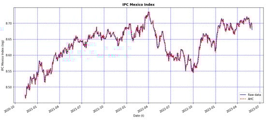 Figure 3. Graphs depicting the AHC model’s forecast using the testing set of the closing price of the IPC (red line) and the original data (blue line).
 - 2
- Figure 4 shows the residuals of the model. The residuals display a satisfactory homogeneous distribution, reinforcing the claim that the model is behaving well.
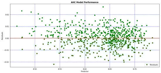 Figure 4. Residuals of the AHC model.
 - 3
- Figure 5 illustrates the behavior of the relative error with a mean and a SD; this shows how the results of the test data have kept a low error rate and low noise or residual variation.
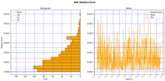 Figure 5. Behavior of the relative error of the AHC model.
We determined the R-square, which measures the performance of a model, based on how well the original output was replicated. In this sense, Table 7 shows the sum of squares and the R-square using the testing set of all the indices. From this table, we can observe that not all the values of the R-square are as good as expected, like the cases of the DAX and the NDX. Nevertheless, for the rest of the indices, the R-square of the testing model is satisfactory and for some cases is high, as in the cases of CAC, the DJIA and the IPC. Table 8 shows some descriptive statistics of the relative error of the testing set. From this table, we can see that, in general, the results of these statistics are good; in the cases of the DJIA and IPC, they have the smallest mean of the relative error with a value.
Table 7.
Statistical measures of the sum of squares and the R-square of the AHC model for the eight indices.
Table 8.
Descriptive statistics of the relative error of the AHC model for the eight indices.
5.2. Model Comparison with GA
Similarly to the previous Section 5.1, some of the results are included here, specifically the results of the IPC index. The complete results for the rest of the indices are provided in Section S2 of the Supplementary Material. In this regard, Table 9 presents the coefficients computed for the IPC model using the GA. In addition, Figure 6 depicts the error behavior through the computation of the 25 generations. Figure 7 shows the forecast using the testing set and compares the original values against the predicted values. Table 10 shows the sum of squared and the R-square of the model performance using the testing set of all the indices. Furthermore, Table 11 illustrates some descriptive statistics of the relative error of the testing sets.
Table 9.
Computed GA genotype with the coefficients (genes) for the IPC model.
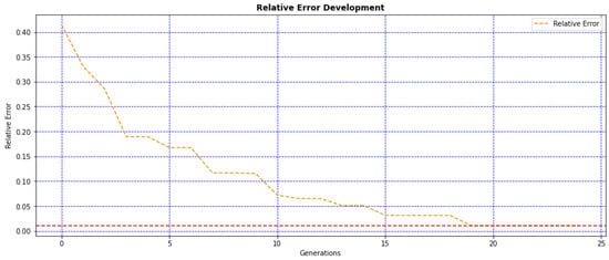
Figure 6.
IPC error behavior through 25 generations.
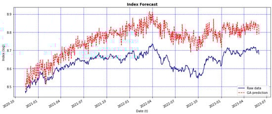
Figure 7.
Graphs depicting the GA model’s forecast using the testing set of the closing price of the IPC (red line) and the original data (blue line).
Table 10.
Statistical measures of the sum of squares and the R-square of the GA model for the eight indices.
Table 11.
Descriptive statistics of the relative error of the GA model for the eight indices.
By contrasting the results obtained from the AHC and the GA models, it can be remarked that, at first hand, the GA has the following advantages over the AHC algorithm:
- It has the capacity to perform a global search, since this method can explore the entire search space and can find global optima in complex spaces.
- It can find a solution via exploration, searching new areas of the solution space and thus focusing on specific areas.
- Its stochastic characteristic allows it to escape local optima.
On the other hand, despite these advantages, the performance of the AHC algorithm makes evident some of the disadvantages of the GA:
- It requires a high computational intensity and thus can be computationally expensive for complex problems and large solution spaces, requiring a significant amount of computational resources and time.
- It can converge prematurely to suboptimal solutions.
- Its performance is sensitive to the choice of parameters, making it susceptible improper tuning, and its optimal parameter tuning can be challenging.
- Due to its stochastic nature, the results can be more susceptible to white noise.
Finally, considering these disadvantages and the results summarized in Table 12 (columns extracted from Table 7, Table 8, Table 10 and Table 11), we can conclude that for the objectives of this research, the AHC algorithm has proven to be a preferable alternative to the GA method.
Table 12.
Comparison of the statistics of the relative error for the eight indices.
Using the data from Table 12, a Wilcoxon signed-rank test was conducted. The p-values are smaller than an alpha of 5%; therefore, statistical significant differences exist between the two methods. This further strengthens the assertion that the AHC algorithm outperforms the GA model. The outcomes of the Wilcoxon signed-rank test are presented in Table 13.
Table 13.
Results of the Wilcoxon signed-rank test for the two methods.
5.3. Cross-Reference Comparison
In addition to the evaluation made in Section 5.2, a further cross-reference [6,7,8,9,10,11,12] comparison against the results obtained in Section 5.1 is presented here. In this respect, Table 14 summarizes some of the results found in the literature and compares them to the results of the forecast using our AHC algorithm.
Table 14.
Cross-reference comparison against the AHC model’s results from the testing sets.
From Table 14, we can state that the AHC algorithm offers promising results. The forecasts reported in the references use the index historical data as input. In our case, to produce the stock market index forecasts, the AHC algorithm makes use not only of the historical data but also considers, for each index, seven country-specific macroeconomic variables. Moreover, our models used a large data size of 17 years (the third largest), besides being tested for eight indices of six different countries. In the cases of the IPC, the DJIA and the CAC, the obtained R-square using the AHC algorithm is comparable to the R-square obtained using the LSTM method, which provided one of the highest R-squares for the DSE with a value of 0.99.
5.4. Complementary Analysis
A complementary analysis is presented here to illustrate the feasibility of using the AHC algorithm forecast in the financial domain. In this sense, the computed forecast of the stock market indices, using the testing set of the closing prices, is used as input to implement a Buy-and-Hold strategy and to compute the Sharpe ratio. The Buy-and-Hold approach uses two moving averages for the index historical data with different time periods: a slow moving average (SMA) and a fast moving average (FMA). There are many common combinations used [26]: 5-day and 20-day averages, 12 and 24, 10 and 30, 10- and 50-day and so forth. For the development of the current experiments, we used the pair 10-day FMA and 30-day SMA. Figure 8 shows the frames of the Buy-and-Hold strategy for the model of the IPC forecast computed in Section 5.1. From this figure, it is possible to see the intersects between the SMA and FMA frames. The outcomes for the Buy-and-Hold strategy for the rest of the indices are included in Section S3 of the Supplementary Material. In addition, Table 15 shows the values of the computed return, volatility and the Sharpe ratio for the forecast period of each index.
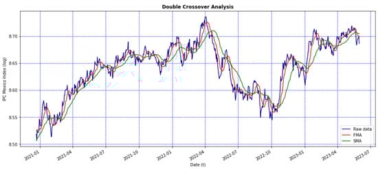
Figure 8.
Curves of the IPC forecast (blue line), with the 10-day FMA (red line) and 30-day SMA frames (green line).
Table 15.
Financial analysis with the computed return, volatility and Sharpe ratio for the forecast of the stock market indices using the testing set of the closing price.
6. Conclusions and Future Work
Through this research, different experiments are offered to evaluate the capabilities of the AHC algorithm as a new supervised machine learning algorithm that can effectively satisfy the objective stated in [2]. The final forecast models obtained by the AHC algorithm provide very encouraging results; for example, in the case of the IPC Mexico stock market index, the R-square is 0.9806, with a mean relative error of . Moreover, the experiments surpass the objective, considering that, among the results, we obtained a series of good forecasts covering months and in some cases even years. Additionally, we worked on eight different stock market indices from six countries, using 17 years of historical data to cover at least one short economic cycle, employing eight MEVs (including the corresponding index) to produce the prediction model of each rate.
As a main contribution, the new algorithm complies with the following properties: it is adaptable and dynamic, and its topology is reconfigurable. Given these properties, the new algorithm can be applied to different approaches or systems that require simulation analysis using time series. Thus, the AHC algorithm provides an alternative tool to financial analysts to produce forecasting scenarios comparable to existing state-of-the-art methods. The AHC algorithm, as a new machine learning technique, opens new research windows in the following directions:
- Improving financial forecasts. Taking into account that our results are evaluated by applying an out-of-sample forecast, changing this approach to a one-day-ahead forecast can improve the performance of the predictions.
- Extending the comparison with other state-of-the-art methods. An extensive assessment of the performance of the new AHC algorithm against other techniques, such as random forest, neural networks, multilayer perceptrons, long short-term memory neural networks and genetic programming, can be carried out.
- Exploring other types of substitutions for the AHC halogenations. Specific kinds of polynomial expressions are used to produce the halogenations for the AHC algorithm; these expressions were chosen based on empirical reasons, leaving space to explore other types of substitutions to yield the halogenations while forming the compounds.
- Increasing and diversifying the application of the AHC algorithm to other fields. One immediate natural application is electricity load forecasting, considering that this task is also based on time series prediction [27]. Another usage that in recent years has gained importance due to its relevance in the medical field is image and pattern recognition, such as cancer detection or kidney stone identification [28]. Further applications where the original AHN algorithm proved to be efficient can be tested, such as signal processing, facial recognition, motor controller and intelligent control systems for robotics, among many other possibilities.
- Extending the analysis of the results. An exhaustive examination of the results can be undertaken regarding more specific aspects, such as model robustness, variation in the results over time and consistency across countries.
The main challenge along our research was to design a new algorithm based on the AON framework, keeping the main attributes of the former AHN topology and, at the same time, introducing new properties to eliminate the usage of gradient descent (used to optimize the position and/or number of molecules), hence reducing the computational time. In this regard, we present a solution that includes two key elements: (a) a new topology inspired by a different functional group by which AHN was originally motivated, and (b) the inclusion of PCA, which plays a key role in the implementation of AHC, since it makes the new algorithm’s time complexity independent of the number of features.
Supplementary Materials
The following supporting information can be downloaded at: https://www.mdpi.com/article/10.3390/bdcc8040034/s1.
Author Contributions
Conceptualization, E.G.-N.; methodology and validation, E.G.-N., L.A.T. and M.K.; formal analysis, E.G.-N., L.A.T. and M.K.; investigation, E.G.-N.; resources and data curation, E.G.-N. and L.A.T.; writing—original draft preparation, E.G.-N.; writing—review and editing, E.G.-N., L.A.T. and M.K.; visualization, E.G.-N.; supervision and project administration, L.A.T.; funding acquisition, E.G.-N. and L.A.T. All authors have read and agreed to the published version of the manuscript.
Funding
The authors would like to acknowledge the financial support of Tecnologico de Monterrey, Mexico, in the production of this work.
Institutional Review Board Statement
Not applicable.
Informed Consent Statement
Not applicable.
Data Availability Statement
Data sharing is available at: https://ieee-dataport.org/documents/datasets-stock-market-indices (accessed on 1 March 2024); https://dx.doi.org/10.21227/yvfx-n484 (accessed on 1 March 2024).
Acknowledgments
Supported by ITESM-CEM and CONAHCyT.
Conflicts of Interest
The authors declare no conflicts of interest. The funders had no role in the design of the study; in the collection, analyses, or interpretation of data; in the writing of the manuscript; or in the decision to publish the results.
References
- Elliott, G.; Timmerman, A. Handbook of Economic Forecasting; Elsevier: Oxford, UK, 2013; Volume 1. [Google Scholar]
- González, E.; Trejo, L.A. Artificial Organic Networks Approach Applied to the Index Tracking Problem. In Advances in Computational Intelligence, Proceedings of the 20th Mexican International Conference on Artificial Intelligence, MICAI 2021, Mexico City, Mexico, 25–30 October 2021; LNCS (LNAI); Springer: Cham, Switzerland, 2021. [Google Scholar]
- Salman, O.; Melissourgos, T.; Kampouridis, M. Optimization of Trading Strategies Using a Genetic Algorithm under the Directional Changes Paradigm with Multiple Thresholds. In Proceedings of the 2022 IEEE Congress on Evolutionary Computation (CEC), Padua, Italy, 18–23 July 2022. [Google Scholar] [CrossRef]
- Salman, O.; Kampouridis, M.; Jarchi, D. Trading Strategies Optimization by Genetic Algorithm under the Directional Changes Paradigm. In Proceedings of the 2022 IEEE Congress on Evolutionary Computation (CEC), Padua, Italy, 18–23 July 2022. [Google Scholar] [CrossRef]
- Ayyıldız, N. Predicting Stock Market Index Movements With Machine Learning; Ozgur Press: Şehitkamil/Gaziantep, Turkey, 2023. [Google Scholar]
- Saboor, A.; Hussain, A.; Agbley, B.L.Y.; ul Haq, A.; Ping Li, J.; Kumar, R. Stock Market Index Prediction Using Machine Learning and Deep Learning Techniques. Intell. Autom. Soft Comput. 2023, 37, 1325–1344. [Google Scholar] [CrossRef]
- Aliyev, F.; Eylasov, N.; Gasim, N. Applying Deep Learning in Forecasting Stock Index: Evidence from RTS Index. In Proceedings of the 2022 IEEE 16th International Conference on Application of Information and Communication Technologies (AICT), Washington, DC, USA, 12–14 October 2022. [Google Scholar] [CrossRef]
- Ding, Y.; Sun, N.; Xu, J.; Li, P.; Wu, J.; Tang, S. Research on Shanghai Stock Exchange 50 Index Forecast Based on Deep Learning. Math. Probl. Eng. 2022, 2022, 1367920. [Google Scholar] [CrossRef]
- Haryono, A.T.; Sarno, R.; Sungkono, R. Stock price forecasting in Indonesia stock exchange using deep learning: A comparative study. Int. J. Electr. Comput. Eng. 2024, 14, 861–869. [Google Scholar] [CrossRef]
- Pokhrel, N.R.; Dahal, K.R.; Rimal, R.; Bhandari, H.N.; Khatri, R.K.C.; Rimal, B.; Hahn, W.E. Predicting NEPSE index price using deep learning models. Mach. Learn. Appl. 2022, 9, 100385. [Google Scholar] [CrossRef]
- Singh, G. Machine Learning Models in Stock Market Prediction. Int. J. Innov. Technol. Explor. Eng. 2022, 11, 18–28. [Google Scholar] [CrossRef]
- Harahap, L.A.; Lipikorn, R.; Kitamoto, A. Nikkei Stock Market Price Index Prediction Using Machine Learning. J. Phys. Conf. Ser. 2020, 1566, 012043. [Google Scholar] [CrossRef]
- Ponce, H. A New Supervised Learning Algorithm Inspired on Chemical Organic Compounds. Ph.D. Thesis, Instituto Tecnológico y de Estudios Superiores de Monterrey, Mexico City, Mexico, 2013. [Google Scholar]
- Ponce, H.; Ponce, P.; Molina, A. Artificial Organic Networks: Artificial Intelligence Based on Carbon Networks, 1st ed.; Springer: Berlin/Heidelberg, Germany, 2014. [Google Scholar]
- Ponce, H.; Gonzalez, G.; Morales, E.; Souza, P. Development of Fast and Reliable Nature-Inspired Computing for Supervised Learning in High-Dimensional Data. In Nature Inspired Computing for Data Science; Springer: Cham, Switzerland, 2019; pp. 109–138. [Google Scholar]
- Ponce, H.; Miralles, L.; Martínez, L. Artificial hydrocarbon networks for online sales prediction. In Advances in Artificial Intelligence and Its Applications, Proceedings of the 14th Mexican International Conference on Artificial Intelligence, MICAI 2015, Cuernavaca, Morelos, Mexico, 25–31 October 2015; Springer: Cham, Switzerland, 2015. [Google Scholar]
- Ayala-Solares, J.R.; Ponce, H. Supervised Learning with Artificial Hydrocarbon Networks: An open source implementation and its applications. arXiv 2020, arXiv:2005.10348. [Google Scholar] [CrossRef]
- Xue, H.; Song, Z.; Wu, M.; Sun, N.; Wang, H. Intelligent Diagnosis Based on Double-Optimized Artificial Hydrocarbon Networks for Mechanical Faults of In-Wheel Motor. Sensors 2022, 22, 6316. [Google Scholar] [CrossRef] [PubMed]
- Ponce, H.; Acevedo, M. Design and Equilibrium Control of a Force-Balanced One-Leg Mechanism. In Advances in Computational Intelligence, Proceedings of the 17th Mexican International Conference on Artificial Intelligence, MICAI 2018, Guadalajara, Mexico, 22-27 October 2018; Springer: Cham, Switzerland, 2018. [Google Scholar]
- Ponce, H.; Acevedo, M.; Morales, E.; Martínez, L.; Díaz, G.; Mayorga, C. Modeling and Control Balance Design for a New Bio-inspired Four-Legged Robot. In Advances in Soft Computing, Proceedings of the 18th Mexican International Conference on Artificial Intelligence, MICAI 2019, Xalapa, Mexico, 27 October–2 November 2019; Springer: Cham, Switzerland, 2019. [Google Scholar]
- Ponce, H.; Ponce, P.; Molina, A. Stochastic parallel extreme artificial hydrocarbon networks: An implementation for fast and robust supervised machine learning in high-dimensional data. Eng. Appl. Artif. Intell. 2020, 89, 103427. [Google Scholar] [CrossRef]
- Ponce, H.; Martínez, L. Interpretability of artificial hydrocarbon networks for breast cancer classification. In Proceedings of the 2017 International Joint Conference on Neural Networks (IJCNN), Anchorage, AK, USA, 14–19 May 2017; IEEE: Piscataway, NJ, USA, 2017. [Google Scholar]
- Ponce, H.; Bravo, M. A Novel Design Model Based on Genetic Algorithms. In Proceedings of the 2011 10th Mexican International Conference on Artificial Intelligence, Puebla, Mexico, 26 November–4 December 2011. [Google Scholar]
- González, E.; Trejo, L.A. Datasets of Stock Market Indices. 2024. Available online: https://ieee-dataport.org/documents/datasets-stock-market-indices (accessed on 1 March 2024).
- González, E. AHC Related Code. Available online: https://github.com/egonzaleznez/ahc (accessed on 1 March 2024).
- Murphy, J.J. Technical Analysis Financial Markets; New York Institute of Finance: New York, NY, USA, 1999. [Google Scholar]
- Zuniga-Garcia, M.A.; Santamaría, G.; Arroyo, G.; Batres, R. Prediction interval adjustment for load-forecasting using machine learning. Appl. Sci. 2019, 9, 5269. [Google Scholar] [CrossRef]
- Lopez-Tiro, F.; Flores, D.; Betancur, J.P.; Reyes, I.; Hubert, J.; Ochoa, G.; Daul, C. Boosting Kidney Stone Identification in Endoscopic Images Using Two-Step Transfer Learning. In Advances in Soft Computing, Proceedings of the 22nd Mexican International Conference on Artificial Intelligence, MICAI 2023, Yucatán, Mexico, 13–18 November 2023; LNCS (LNAI); Springer: Cham, Switzerland, 2023. [Google Scholar] [CrossRef]
Disclaimer/Publisher’s Note: The statements, opinions and data contained in all publications are solely those of the individual author(s) and contributor(s) and not of MDPI and/or the editor(s). MDPI and/or the editor(s) disclaim responsibility for any injury to people or property resulting from any ideas, methods, instructions or products referred to in the content. |
© 2024 by the authors. Licensee MDPI, Basel, Switzerland. This article is an open access article distributed under the terms and conditions of the Creative Commons Attribution (CC BY) license (https://creativecommons.org/licenses/by/4.0/).