Article

BNMI-DINA: A Bayesian Cognitive Diagnosis Model for Enhanced Personalized Learning

1
Department of Computer Science and Technology, Anhui University, Hefei 230601, China
2
Department of Mathematics and Information Science, Guangzhou University, Guangzhou 510006, China
*
Author to whom correspondence should be addressed.
Big Data Cogn. Comput. 2024, 8(1), 4; https://doi.org/10.3390/bdcc8010004
Submission received: 17 November 2023 / Revised: 16 December 2023 / Accepted: 26 December 2023 / Published: 29 December 2023

Abstract

:
In the field of education, cognitive diagnosis is crucial for achieving personalized learning. The widely adopted DINA (Deterministic Inputs, Noisy And gate) model uncovers students’ mastery of essential skills necessary to answer questions correctly. However, existing DINA-based approaches overlook the dependency between knowledge points, and their model training process is computationally inefficient for large datasets. In this paper, we propose a new cognitive diagnosis model called BNMI-DINA, which stands for Bayesian Network-based Multiprocess Incremental DINA. Our proposed model aims to enhance personalized learning by providing accurate and detailed assessments of students’ cognitive abilities. By incorporating a Bayesian network, BNMI-DINA establishes the dependency relationship between knowledge points, enabling more accurate evaluations of students’ mastery levels. To enhance model convergence speed, key steps of our proposed algorithm are parallelized. We also provide theoretical proof of the convergence of BNMI-DINA. Extensive experiments demonstrate that our approach effectively enhances model accuracy and reduces computational time compared to state-of-the-art cognitive diagnosis models.

1. Introduction

The emergence of the online education industry has revolutionized traditional educational approaches. Leveraging information technology, online education offers students convenient access to a vast array of courses and learning materials, thus promoting resource sharing and ensuring educational equity. However, with the exponential growth of available learning resources, accurately assessing a student’s mastery level of specific skills and knowledge has become a pressing challenge. Cognitive diagnosis models (CDMs), initially introduced by [1], have been developed to quantify the latent abilities that significantly impact students’ performance. CDMs [2,3] have gained widespread recognition and interest from both academic and industry domains by providing insights into the cognitive skills underlying students’ overall scores [4].
The DINA (Deterministic Inputs, Noisy And gate) model [5] is recognized as a prominent cognitive diagnosis approach, which effectively integrates the Q-matrix and students’ response patterns to assess their mastery level and identify potential error patterns within each knowledge point. By employing statistical techniques such as maximum likelihood estimation [6], the DINA model equips educators with a comprehensive cognitive diagnostic tool, enabling the formulation of personalized teaching strategies that cater to individuals’ performance across diverse knowledge points.
However, the DINA model faces various challenges in practical applications. Firstly, it employs discrete variables to indicate whether a student has mastered a particular knowledge point, with 1 representing mastery and 0 representing non-mastery. This approach becomes problematic in subject areas that require continuous assessment, such as art evaluation in domains like painting and music. Secondly, the DINA model is unable to account for the interrelatedness between knowledge points within questions, which limits its effectiveness in capturing the comprehensive cognitive skills of students. Thirdly, the training of traditional DINA models becomes computationally expensive due to the use of large datasets, which may contain millions of student records and question items from online education platforms.
In this paper, to address these aforementioned challenges, we propose a precise and efficient cognitive diagnosis approach called BNMI-DINA (Bayesian Network-based Multiprocess Incremental DINA). By incorporating the probabilistic inference and uncertainty modeling capabilities of Bayesian networks, we can more accurately assess the mastery level of students’ knowledge points. Additionally, we expedite the training process through parallel computation for parameter estimation. The key contributions of this paper are outlined as follows:
  • To the best of our knowledge, we are the first to integrate Bayesian networks into the DINA model to obtain continuous mastery levels for knowledge points and account for their interdependence. Our proposed model overcomes the limitation of the DINA model by considering the dependencies between knowledge points, enabling a more comprehensive evaluation of students’ cognitive skills.
  • We propose a parallelization method that effectively parallelizes the key steps of our BNMI-DINA model, thereby significantly reducing the computational burden associated with model training. This parallelization enables the application of BNMI-DINA to large datasets. Additionally, we provide theoretical proof of the convergence of BNMI-DINA, establishing its validity and ensuring reliable results.
  • We conduct extensive experiments using real datasets to validate the performance of BNMI-DINA. The results of our experiments demonstrate the superiority of BNMI-DINA when compared to other baseline models. Specifically, BNMI-DINA outperforms the alternatives in terms of both model accuracy and training efficiency, solidifying its position as a highly effective and efficient cognitive diagnosis approach.
The remainder of this paper is organized as follows: in Section 2, we conduct a comprehensive review of commonly used approaches in cognitive diagnosis and Bayesian networks. In Section 3, we present a detailed overview of the DINA model and provide necessary background knowledge. Next, in Section 4 and Section 5, we propose our novel approach and provide a proof of its convergence, respectively. Section 6 showcases the experimental results, which demonstrate the effectiveness of our approach. Finally, in Section 7, we conclude the paper by summarizing the key findings and discussing avenues for future research.

2. Related Work

Cognitive diagnosis, initially proposed by educational psychologists for psychological measurement, has its roots in the 1990s. Frederiksen et al. [7] were credited with formally introducing the theories and concepts related to cognitive diagnosis in 1993, while Nichols et al. [8] further provided a comprehensive summary and categorization of these theories and concepts in 1995. Leighton et al. [9] considered CDM as a promising evaluation model that can delve into the underlying structure of a field and identify problems and areas that need improvement in 2007. Lee et al. [10] proposed that tests informed by the Cognitive Diagnosis Algorithm (CDA) can specify the underlying knowledge structure behind the overall test score, and this specification can serve as feedback to meet individual and group needs through remedial instruction and improve instruction to enhance learning and competency in 2009. As a diagnostic approach to assessment, CDA needs statistical and mathematical models to operationalize the assumptions. CDMs are psychometric models that make use of an item response pattern in order to determine test-takers’ cognitive abilities [11]. In all CDA studies, the selection of statistical models is a critical step and requires close attention and consideration of model selection criteria. However, in most CDA studies, tests applying a predetermined CDM are chosen based on the characteristics of the model and the practicality issue. So Li et al. [12] carefully studied the considerations required for CDM selection for reading comprehension tests and found that when the relationship between cognitive skills is not completely clear, it is safe to use a saturated (more complex) CDM, which can flexibly adapt to different types of relationships between skills in 2016. Currently, cognitive diagnosis can be defined in both broad and narrow terms. Broadly speaking, cognitive diagnosis leverages modern technologies such as computer-based testing and statistical methods to assess users’ cognitive abilities and structures [13,14]. On the other hand, in a narrower sense, cognitive diagnosis classifies users based on their mastery level of specific knowledge points, with the classification results used for personalized educational interventions.
The application of cognitive diagnosis in the education industry has led to a shift towards personalized education in traditional online classrooms [15,16]. Cognitive diagnosis models can be differentiated from two perspectives. Firstly, they can be classified as continuous diagnosis models or discrete diagnosis models, depending on their ability to diagnose continuous scores. Secondly, cognitive diagnosis models can be classified based on their approach to handling dimensions of students’ cognitive abilities. This categorization results in one-dimensional skill diagnosis models and multidimensional skill diagnosis models. Currently, there are more than 60 cognitive diagnosis models available. These models include the rule-based model, attribute hierarchy model, Deterministic Inputs, Noisy And gate (DINA) model, as well as various variations [17,18] such as the Fuzzy CDF model [19]. Improved versions of the DINA model, such as the HO-DINA [20], P-DINA [21], G-DINA [22], and Incremental DINA (I-DINA) model [23], are also among the existing models used in cognitive diagnosis research.
The history of Bayesian networks dates back to the early 1980s. In 1988, Pearl et al. [24] first introduced the fundamental concepts and inference methods of Bayesian networks in their seminal paper. Notably, Pearl’s work also introduced the concept of the “causal graph”, which expanded probabilistic graph models to incorporate causal relationships, thereby establishing the groundwork for further development. In the 1990s, research in the field expanded from representation issues to encompass inference and learning [25], making Bayesian networks more practical in various applications. With the advancement of computational power and the exponential growth of data in the 21st century, Bayesian networks have found widespread application in diverse domains such as medicine [26], finance [27], and natural language processing [28]. Research in the field has also made significant progress in reasoning, learning, and the application of Bayesian networks [29].
In recent research, the integration of Bayesian networks and the DINA model has gained attention, with notable applications in student modeling, knowledge tracing, and skill topology. For instance, Conati et al. [30] applied Bayesian networks to the Andes project [31], an intelligent educational system focused on Newtonian physics, to model uncertainty within students’ reasoning and learning processes. In the domain of knowledge tracing [32], Pelánek [33] introduced Bayesian Knowledge Tracing (BKT), which employed Bayesian networks to infer latent student variables within knowledge-tracing models. Furthermore, Käser et al. [32] utilized dynamic Bayesian networks (DBN) to model skill topology in knowledge tracking. While these works have made significant contributions to the application of Bayesian networks, their main focus lies in student modeling, knowledge tracing, and skill topology. In parallel, recent breakthroughs in asynchronous federated meta-learning, exemplified by AFMeta, have effectively addressed issues such as straggler and over-fitting, resulting in a substantial improvement in model performance and a notable reduction in learning time [34]. In the field of education-based information analysis, the examination of student learning assessment methods based on text data has emerged as a crucial research area. Liu et al. [35] introduced an innovative learning evaluation method based on real-time text data attributes, overcoming the limitations of traditional evaluation methods. The outcomes highlight the superior effectiveness of utilizing real-time attribute text data in measuring students’ learning outcomes.
Table 1 provides a concise overview of the key aspects explored in order to clearly demonstrate the scope of the related work.
In contrast, our work delves deeper into cognitive diagnosis problems. We not only incorporate a Bayesian network to capture the dependency relationship between knowledge points but also enhance computational efficiency, especially for large datasets.

3. Preliminaries

In this section, we will provide a detailed description of the DINA model and its corresponding symbolic representation.
As shown in Figure 1, the DINA model diagnoses students’ cognitive abilities by utilizing the question-knowledge matrix Q and the user-question response matrix R. Compared to other cognitive diagnosis models, DINA is characterized by its simplicity, flexibility, and ease of implementation and understanding.
In this model, the variable q υ k represents the assessment of knowledge point k by question v, r u v represents the score of student u on question v, and η u v represents the latent response of student u on question v. Additionally, the mastery level of the assessed knowledge points by students is described as a multi-dimensional [36] knowledge point mastery vector
α u = α u 1 , α u 2 , , α u K ,
where α u k = 1 represents that student u has mastered knowledge point k. Otherwise, α u k = 0 . The main notions are summarized in Table 2.
The core formula of the model is
η u v = k = 1 K α u k q υ k ,
where the exponential structure represents the logical “AND” relationship among the knowledge points being assessed. The model introduces the slip parameter s v and the guess parameter g v to more accurately estimate the students’ mastery status. The slip parameter s v represents the probability of giving a wrong response due to error, given that the student has mastered the knowledge point. The guess parameter g v represents the probability of giving a correct response through guessing or luck when the student has not mastered the knowledge point. The definitions of the above two parameters are as follows:
g v = P ( r u v = 1 | η u v = 0 ) ,
s v = P ( r u v = 0 | η u v = 1 ) .
By combining the slip factor and guess factor, it is possible to estimate the probability of a student answering a question correctly. Given the multi-dimensional knowledge point mastery vector α u , the probability of student u answering question v correctly is as follows:
P r u υ = 1 α u = g υ 1 η u υ 1 s υ η u υ .
Through derivation, the DINA model can determine the joint probability of a student’s response pattern for all questions. In cases where the student’s multi-dimensional knowledge point mastery vector is known, the model further seeks to estimate the values of the slip parameter s v and guess parameter g v . However, in practical scenarios, the student’s multi-dimensional knowledge point mastery vector is often unknown. Therefore, the marginal likelihood function and the maximum likelihood estimation algorithm are introduced to estimate the values of s v and g v .
Finally, by maximizing the posterior probability of the student’s question responses and incorporating the estimated slip and guess parameters, the DINA model can derive the estimated values of the student’s multi-dimensional knowledge point mastery vector. This data-driven and probabilistic approach offered by the DINA model enables accurate assessment of students’ knowledge mastery and provides valuable support for personalized learning.
However, the DINA model encounters several challenges in practical applications. Firstly, it uses discrete variables to denote whether a student has mastered the related knowledge points with 1 as acquired and 0 as not acquired [37]. This approach poses difficulties when dealing with subject areas that demand continuous assessment, such as art evaluation in domains like painting and music. Secondly, questions may contain knowledge points that are related to each other, and the DINA model fails to handle this case. Thirdly, millions of student records and question items are collected from online education platforms, which brings significant computational costs for the training of traditional DINA models.

4. Design of BNMI-DINA Model

This section presents a comprehensive outline of our proposed BNMI-DINA model, which aims to address the limitations of the traditional DINA model mentioned earlier.

4.1. Framework Overview

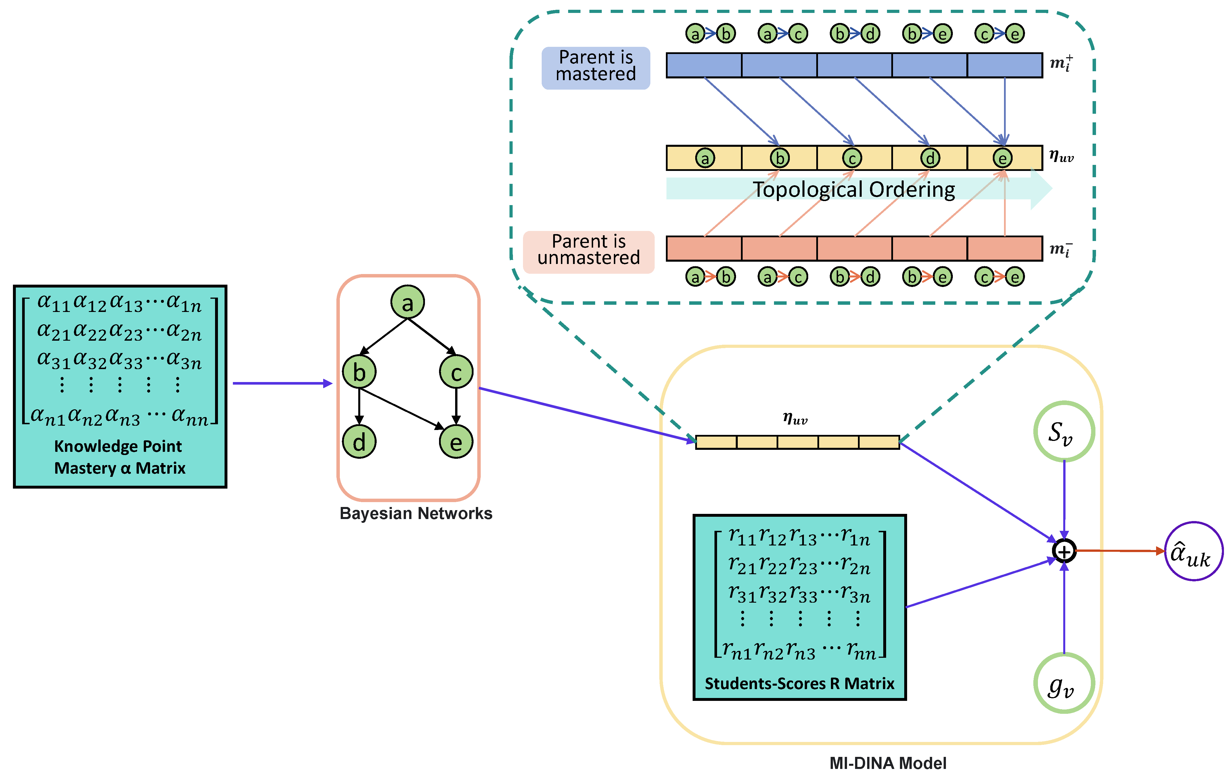
As shown in Figure 2, BNMI-DINA mainly contains two modules, namely, a Bayesian network module and an MI-DINA module. Initially, the student’s knowledge point mastery is represented by the α matrix, which serves as the input for the Bayesian network. Through Bayesian network modeling, the hierarchical relationships among knowledge points are revealed. By computing the mastery probability for each knowledge point using the posterior probabilities, a vector of knowledge point mastery probabilities is generated. Subsequently, this vector is combined with the student’s score matrix R and input into the DINA model. By taking into account the slip factor and guess factor, the DINA model estimates the matrix of the student’s knowledge point mastery. This integrated methodology provides educators with a more precise understanding of students’ mastery levels across different knowledge points, enabling them to deliver targeted instruction and guidance effectively.

4.2. Bayesian Network Module

We first introduce the Bayesian network module of the model. In the Bayesian network module, each node represents a knowledge point, and the directed arrows represent the dependency relationships between knowledge points [38]. In Figure 2, for example, node b represents a knowledge point b, and node b is a successor of node a, indicating that knowledge point a is a prerequisite for knowledge point b. Based on the obtained matrix of knowledge point mastery, the number of students who scored 1 on each knowledge point is counted and then divided by the total number of students to estimate the prior probability o u k of student u mastering knowledge point k. The calculation formula of o u k is as follows:
o u k = β ( k , s c = 1 ) U ,
where s c is the student’s score on a certain knowledge point, and the β function is defined as the count of students with a score of 1 (i.e., s c = 1 ) for knowledge point k.
Next, through the established Bayesian network, the individual knowledge level γ u k = P ( α u k = 1 ) of student u on knowledge point k is obtained by analyzing the number of parent nodes for each node [39]. Different scenarios are discussed below, based on the number of parent nodes for each node.
No parent nodes: when a node has no parent nodes, such as node a in Figure 2, it means that the knowledge point represented by node a has no predecessors. Thus, students are able to begin learning this particular knowledge point without any prior knowledge. Consequently, the mastery of this attribute by students is unaffected by any other attributes. Therefore, the calculation formula for the probability of mastering this knowledge point attribute is as follows:
γ u k = o u k .
One parent node: when a node has one parent node, such as node x = c in Figure 2, to calculate the posterior probability more accurately, we introduce positive factor m u k | x + and negative factor m u k | x , defined as follows:
m u k | x + = P ( α u k = 1 | α u x = 1 ) m u k | x = P ( α u k = 1 | α u x = 0 )
If the value of m u k | x is higher, even if knowledge point x is not mastered, it is more likely to consider that the student has mastered knowledge point k. Therefore, in the student’s learning process, the dependency of mastering k on mastering x is lower. If the value of m u k | x + is lower, even if the parent x is mastered, there is a tendency not to master attribute k. Therefore, for students, attribute k is considered to be more difficult. In simpler terms, the better a student masters the parent attribute, the better they will master the child attribute. Therefore, the probability calculation formula for the mastery of this knowledge point attribute is as follows:
γ u k = m u k | x + γ u x + m u k | x ( 1 γ u x ) .
Multiple parent nodes: when a node has multiple parent nodes, such as node e in Figure 2, we can analyze it as follows. Firstly, if the mastery level of one of the parent nodes is higher, then the mastery level of its child node should also be higher. In other words, for a knowledge point P ( α u k = 1 | α u x 1 , , α u x n ) , if the mastery level of parent node x j ( 1 j n ) is higher, then P is larger. Secondly, if one of the parent nodes is not mastered or has a very low mastery level, then we should assume that the child node is also not mastered or has a low mastery level. If one of the parent nodes is not mastered, then we tend to believe that the child node has also not been mastered. Considering these properties, it is found that the geometric mean can well describe the above properties. Therefore, the following formula can be obtained as follows:
P ( α u k = 1 | α u x 1 , , α u x n ) = z = 1 n m u k | x z ( α u x z ) n .
For each joint probability of parent nodes x 1 , x 2 , , x n , we have:
P ( α u x 1 , , α u x n ) = z = 1 n ( ( 1 α u x z ) ( 1 γ u x z ) + α u x z γ u x z ) .
Finally, γ u k can be inferred as the expectation of P ( α u k = α u x z ) . Therefore, we can derive the probability calculation formula for the mastery of knowledge point attribute as follows:
γ u k = α u x { 0 , 1 } P ( α u x 1 , , α u x n ) z = 1 n m u k | x z α u x z n .

4.3. MI-DINA Module

We proceed to introduce the MI-DINA module, which is designed to address the limitations of traditional DINA models in terms of parameter estimation and training efficiency, especially when dealing with educational assessments that involve large datasets and complex models. MI-DINA is an innovative parallel cognitive diagnosis model that builds upon the incremental DINA framework. This algorithm leverages the convergence and maximum likelihood estimation properties of the EM algorithm [40] to address parameter estimation issues associated with latent variables [41] and to partition data. The likelihood function for the MI-DINA model is represented by Equation (13). Given the presence of unobservable latent variables within the equation, the EM algorithm is introduced to estimate unknown parameters effectively. The process of the EM algorithm can be summarized into the following four steps:
1.
Perform initialization operations for parameters that cannot be directly observed and estimate model parameter values.
2.
Based on the estimated model parameter values, estimation operations are performed on parameters that cannot be directly observed.
3.
Re-estimate the model parameters based on the parameter values estimated in step 2 that cannot be directly observed.
4.
Repeat steps 2–3 until the parameters converge.
Specifically, in the EM loop iteration process, the main role of E-stepis to use data and existing models to perform estimation operations on parameters, and then use parameter estimates to solve the expected value of the likelihood function.
L ( R ) = u = 1 U L r u = u = 1 U l = 1 D L r u α l P α l ,
where L ( r u ) represents the marginal likelihood of the multidimensional knowledge state vector α u for student u, D = 2 K represents the total number of possible combinations for the multidimensional knowledge state vector α u under the condition that the total number of examined knowledge points is K, i.e., there are 2 K combinations that are mutually independent and do not influence each other. Similarly, P ( α l ) represents the probability of the l-th combination, and its value is 1 2 K , because in the DINA model, it is assumed that these 2 K combinations occur with equal probability. L ( r u | α l ) is defined as follows:
L r u α l = L r u 1 , r u 2 , , r u V α u = α l = v = 1 V P v α u r u v 1 P v α u ( 1 r u v ) ,
where P v α u is a shorthand for Equation (5). The procedure is decribed in Algorithm 1, which mainly contains three steps as follows:
Initialization: in this step, we randomly initialize a set of data
Θ = s 1 , g 1 , s 2 , g 2 , s 3 , g 3 , , s V , g V
followed by conducting the E-step and M-step in the EM algorithm.
E-step: in the DINA model, with the help of the estimated values of s v and g v obtained from the previous iteration, the value of the matrix P ( R α ) = P r u α l U × 2 K is calculated, and at the same time, the value of the target matrix P α l r u U × 2 K is calculated using P ( R α ) . Here, u = 1 , 2 , , U , l = 1 , 2 , , 2 K . However, when dealing with large datasets, the computational time required for the E-step becomes extensive, resulting in slow convergence and low computational efficiency. To address this issue, the MI-DINA model incorporates the concept of the incremental DINA model: the user student population U is divided into multiple disjoint blocks of student populations { U 1 , U 2 , , U N } , and in each iteration of the E-step, the MI-DINA model selects only one of the blocks of student populations to update the target likelihood function for calculating the estimated values of the matrices. Meanwhile, the calculations for the other blocks are skipped, and the likelihood function values obtained from the previous iteration are retained. This ensures computational efficiency by reducing the number of calculations required for parameter estimation.
Algorithm 1 Pseudo-code of MI-DINA cognitive diagnostic process
Input:
    Student-Question score matrix R;
    Question-Knowledge point matrix Q;
Output:
    Estimate of the multidimensional knowledge mastery vector for a student user α ^ u ;
1:
Randomly initialize parameters Θ = { ( s 1 , g 1 ) , ( s 2 , g 2 ) , ( s 3 , g 3 ) , , ( s V , g V ) } ;
2:
Divide the population of student users U in the dataset into multiple disjoint blocks of student user groups { U 1 , U 2 , , U N } ;
3:
t = 1 ;
4:
while  Θ { ( s 1 , g 1 ) , ( s 2 , g 2 ) , ( s 3 , g 3 ) , , ( s V , g V ) } do not converge do
5:
    /* E-step */.
6:
    Random Select n;
7:
    if  U i U n  then
8:
        Compute P ( r u | α l ) t based on ( s t 1 , g t 1 ) ;
9:
    else
10:
         P ( r u | α l ) t P ( r u | α l ) t 1 ;
11:
    end if
12:
    Compute P ( α | R ) t based on P ( R | α ) t ;
13:
    /* M-step */
14:
    /* Perform parallel computation of 4 key parameters using multi-processing. */
15:
    for each l 2 K  do
16:
         I v l ( 0 ) α l : α l q v < q v q v u = 1 U P α l r u ;
17:
         I v l ( 1 ) α l : α l q v = q v q v u = 1 U P α l r u ;
18:
         R v l ( 0 ) α l : α l q v < q v q v u = 1 U P α l r u r i v ;
19:
         R v l ( 1 ) α l : α l q v = q v q v u = 1 U P α l r u r i v ;
20:
    end for
21:
     s ^ v I v l ( 1 ) R v l ( 1 ) I v l ( 1 ) ;
22:
     g ^ v R v l ( 0 ) I v l ( 0 ) ;
23:
     t t + 1 ;
24:
end while
25:
α ^ u = arg   max a P ( α | r u ) ;
26:
return  α ^ u ;
M-step: let log L ( R ) s v = 0 and log L ( R ) g v = 0 to obtain the following expressions for estimating the guessing parameter and slip parameter:
s ^ v = I v l ( 1 ) R v l ( 1 ) I v l ( 1 ) ,
g ^ v = R v l ( 0 ) I v l ( 0 ) ,
where I v l ( 0 ) represents the expected number of students in a population who have the same level of mastery for the l-th knowledge point as the partially-mastery group being tested on the v-th question among the 2 K possible mastery configurations of the knowledge points; R v l ( 0 ) represents the expected number of students in I v l ( 0 ) who answer the v-th question correctly; I v l ( 1 ) and R v l ( 1 ) have similar meanings to I v l ( 0 ) and R v l ( 0 ) , with the difference being that I v l ( 1 ) and R v l ( 1 ) correspond to the expected number of students in the population under the condition that they have fully mastered all knowledge points being tested on the v-th question. Therefore, in M-step, the estimated values u = 1 U P α l r u r u v and u = 1 U P α l r u calculated in E-step can be used to calculate the four key parameters. The calculation formulas of the four key parameters are as follows:
I v l ( 0 ) = α l : α l q v < q v q v u = 1 U P α l r u ,
I v l ( 1 ) = α l : α l q v = q v q v u = 1 U P α l r u ,
R v l ( 0 ) = α l : α l q v < q v q v u = 1 U P α l r u r i v ,
R v l ( 1 ) = α l : α l q v = q v q v u = 1 U P α l r u r i v .
In addition to replacing the complete expectation step with the partial expectation step in the incremental DINA model, the maximization step in MI-DINA model considers the solution process of each key parameter as a subtask and executes multiple subtasks in parallel. The main process waits for all the subprocesses to complete before integrating the results to solve the key parameters. Compared to the incremental DINA model, the MI-DINA model retains its original parameters, ensuring interpretability. Furthermore, the EM algorithm is improved to not only guarantee parameter estimation through iterative methods but also accelerate the overall diagnostic speed of the algorithm.

5. Convergence of BNMI-DINA Model

In this section, we will prove the convergence of our proposed BNMI-DINA model. As previously mentioned, the BNMI-DINA model consists of two modules. In the Bayesian network module, the mastery of the child nodes is determined based on the mastery of the parent node, and samples are generated using a sampling method. This sampling method follows a directed generative process, which does not affect the convergence of the model [42]. Hence, it is only necessary to prove the convergence of the MI-DINA module.
The MI-DINA module employs a partial E-step, as suggested by [43], in order to reduce computation time. In this approach, the entire group of student users, denoted as U, is divided into multiple disjoint student blocks denoted as { U 1 , U 2 , , U N } . During each E-step computation, only one student block, U a U , is processed to update the likelihood function, while the likelihood function values for the remaining blocks are retained from the previous iteration. This partial E-step strategy effectively reduces computational time and enhances the algorithm’s efficiency. Moreover, the M-step is divided into multiple subtasks that can be solved concurrently using parallel computing. Each subtask independently handles key parameters, such as I v l ( 0 ) , I v l ( 1 ) , R v l ( 0 ) and R v l ( 1 ) . By utilizing parallel computing, these subtasks can be executed simultaneously without any interference or mutual impact on their computations. The main process waits for all subprocesses to complete and then integrates their results. Importantly, this parallelized computing approach does not compromise the convergence of the MI-DINA model. Even when incorporating parallel computing, the algorithm is still capable of achieving convergence.
To ensure the validity of the proposed MI-DINA model, it is crucial to demonstrate its convergence to a stable state. Here, we provide a proof of convergence for the MI-DINA model using the EM algorithm.
We aim to prove whether the MI-DINA model can achieve the maximization of the logarithmic likelihood function l ( R ) t through iteration, given the question-knowledge matrix Q and the user-question and score matrix R.
l ( R ) = ln L ( R ) = ln i = 1 u L ( R i ) = i = 1 u ln l = 1 D P ( R i α l ) P ( α l ) = i = 1 u ln l = 1 D z l ( α l ) P ( R i α l ) P ( α l ) z l ( α l ) .
The probability mass function of α l is denoted as z l ( α l ) , so z l ( α l ) also satisfies the constraints 0 z l ( α l ) 1 , l z l ( α l ) = 1 . Therefore, l = 1 D z l ( α l ) P ( R i α l ) P ( α l ) z l ( α l ) can be considered as the expectation of P ( R i α l ) P ( α l ) z l ( α l ) with respect to z l ( α l ) . By applying Jensen’s inequality, we have:
ln l = 1 D z l ( α l ) P ( R i α l ) P ( α l ) z l ( α l ) l = 1 D z l ( α l ) ln P ( R i α l ) P ( α l ) z l ( α l ) .
After substituting the formula into l ( R ) , we obtain:
l ( R ) = i = 1 u ln l = 1 D z l ( α l ) P ( R i α l ) P ( α l ) z l ( α l ) i = 1 u l = 1 D z l ( α l ) ln P ( R i α l ) P ( α l ) z l ( α l ) .
If we let
B ( R ) = i = 1 u l = 1 D z l ( α l ) ln P ( R i α l ) P ( α l ) z l ( α l ) ,
then B ( R ) becomes the lower bound function for l ( R ) . If we can derive B ( R ) = l ( R ) , B ( R ) achieves its maximum value.
According to the properties of Jensen’s inequality, it can be observed that if we set P ( R i α l ) P ( α l ) z l ( α l ) as a constant value, i.e., P ( R i α l ) P ( α l ) z l ( α l ) = c , the inequality in Equation (24) can be replaced by equality. In this case, B ( R ) reaches its maximum value. Therefore, the maximum value of the lower bound function B ( R ) , denoted as m a x B ( R ) , is equivalent to maximizing the log-likelihood function l ( R ) . Hence, in order to maximize l ( R ) , we can maximize B ( R ) . Additionally, let l ( R ) t represent the log-likelihood function at the t-th iteration. To prove the convergence of the algorithm, it is sufficient to demonstrate that l ( R ) t + 1 > l ( R ) t as follows:
l ( R ) t + 1 = m a x B ( R ) t + 1 = i = 1 u l = 1 D z l ( α l ) t + 1 ln P ( R i α l ) t + 1 P ( α l ) z l ( α l ) t + 1 i = 1 u l = 1 D z l ( α l ) t ln P ( R i α l ) t + 1 P ( α l ) z l ( α l ) t i = 1 u l = 1 D z l ( α l ) t ln P ( R i α l ) t P ( α l ) z l ( α l ) t = l ( R ) t .
It is important to note that in Equation (26), as long as P ( R i | α l ) t and P ( R i | α l ) t + 1 are not exactly equal, the first inequality holds. For the model, although in the E-step, the student-user blocks are partitioned, when R i R a , then P ( R i | α l ) t = P ( R i | α l ) t + 1 . However, for R i R a , then P ( R i α l ) t will be updated unless the overall likelihood function has been maximized and the iteration stops. Therefore, unless the iteration has already stopped due to the maximization of the overall likelihood function, P ( R i | α l ) t and P ( R i | α l ) t + 1 cannot be exactly equal, and thus the first inequality holds. The second inequality is guaranteed by the maximization process in the M-step. In conclusion, the MI-DINA model ensures the convergence of the EM step and we also complete the proof of the convergence of the BNMI-DINA model.

6. Experiments

In this section, we evaluate the performance of our approach, BNMI-DINA, in comparison to traditional cognitive diagnosis methods in terms of model accuracy and training efficiency.

6.1. Datasets

The Junyi dataset [44] is obtained from the Junyi Academy Math Practicing Log (Junyi), which includes learning behavior data such as student responses, learning activities, and other learning-related information. To assess the models’ performance on datasets of varying sizes, we split the Junyi dataset and create a new dataset called Junyi-scaled by selecting a small subset.
Dataset Characteristics: Table 3 presents comprehensive statistics for both the original Junyi dataset and the scaled-down Junyi-scaled dataset. The Junyi dataset comprises problem logs and exercise-related data from 10,000 students of the Junyi Academy, with 734 attributes, 734 question items, and 408,057 response logs. On the other hand, Junyi-scaled, which is a subset specifically created for controlled experiments, consists of data from 2400 students, featuring 10 attributes, 10 question items, and 6100 response logs.
Pre-processing: pre-processing the Junyi dataset is a crucial step in ensuring the quality and relevance of the data for training and evaluation purposes. In order to capture the relationships within the educational contents, a knowledge graph is generated using the Junyi dataset. To accomplish this, the edudata tool [1] is employed to extract relations and store the resulting graph data. Additionally, we allocate 80% of the data to the training set and reserve the remaining 20% for the test set.

6.2. Visualizing the Relationship of Knowledge Points

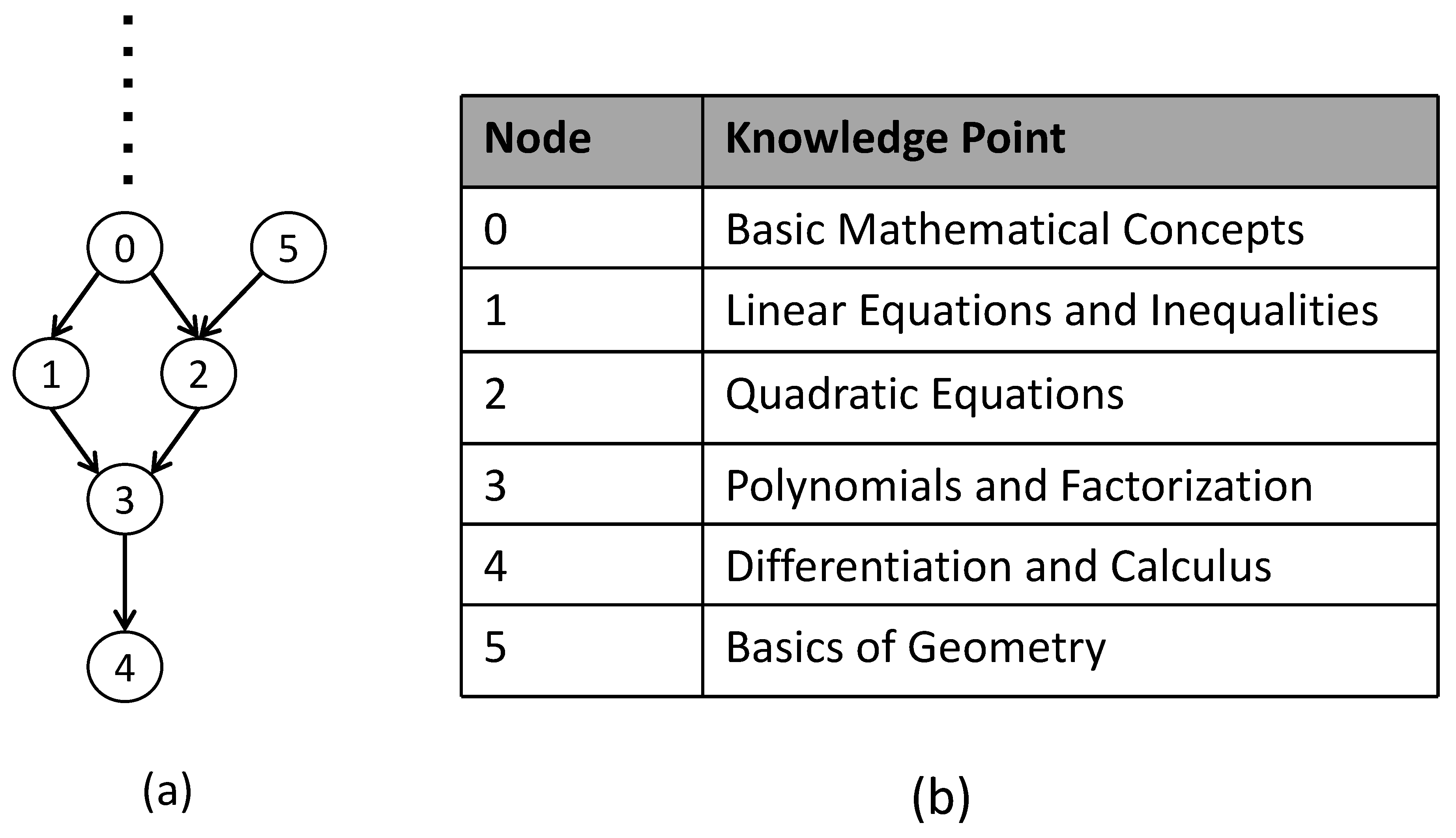
To illustrate the relationship between knowledge points, we utilize specific knowledge points to depict the tree structure within the dataset. We have extracted a small portion of the tree structure from the Junyi dataset, as depicted in Figure 3a. The nodes are numbered from 0 to 5, and the corresponding relationships between the knowledge points are shown in Figure 3b.
In the process of learning mathematics, students typically follow a step-by-step approach to acquire knowledge of predecessor and successor concepts. They start by mastering basic mathematical concepts (node 0). Then, they can directly move on to study linear equations and inequalities (node 1), or master basics of geometry (node 5) for better learning quadratic equations (node 2). Building on the foundation laid in the earlier stages, students then advance to the study of polynomials and factorization (node 3). Finally, students can explore more advanced topics such as differentiation and calculus (node 4). This sequential learning order ensures that students progressively build upon their existing knowledge, allowing for a coherent and structured development of mathematical proficiency.

6.3. Evaluation Metrics

To evaluate the performance of the models, we utilize three key evaluation metrics: accuracy, time, and F1 score [45].
  • Accuracy is calculated as the ratio of successful predictions to the total number of instances in the test set. It quantifies the proportion of correct predictions in relation to the entire test set size.
  • Time refers to the duration of a particular process, measured in seconds. It provides insights into the efficiency of the model in terms of computation time.
  • The F1 score combines precision and recall, offering a comprehensive assessment of the model’s predictions. Precision evaluates the ratio of correct positive predictions, while recall assesses the ratio of correctly predicted positive instances.
The F1 score is calculated as below:
F 1 = 2 × P r e c i s i o n × R e c a l l P r e c i s i o n + R e c a l l ,
where p r e c i s i o n is defined as
P r e c i s i o n = T P T P + F P ,
representing the proportion of correct recommendations, and r e c a l l is defined as:
R e c a l l = T P T P + F N ,
representing the proportion of correctly predicted positive instances. Here, T P is the count of correctly answered recommendations, F P is the count of incorrect recommendations, and F N is the count of correctly answered instances not included in the recommendations.

6.4. Experimental Settings

To assess the effectiveness and feasibility of the proposed BNMI-DINA model and its non-parallel version, we compared them against six alternative algorithms in our study. The first three algorithms chosen for comparison do not incorporate Bayesian networks, while the remaining three algorithms do incorporate Bayesian networks. This approach allows us to evaluate the performance and advantages of the proposed models in comparison to both non-Bayesian and Bayesian network-based approaches.
We compare our model against the following six algorithms: IRT, MF [46], NeuralCD [47], HierIRT [48], HierMF [48], and HierNeuralCD [48]. For score prediction, we set the threshold at 0.5. In the multidimensional latent factor model, we set the hidden dimension n to 3. The dimensions of the fully connected layers in NeuralCD are set to 512, 256, and 1, respectively, as described in [47]. All experiments are conducted on a Linux Ubuntu 20.04.6 server, equipped with two 2.60 GHz Intel Xeon E5-2650v2 CPUs and 252 GB of RAM. This server configuration ensured the reliability and efficiency of the experimental setup.

6.5. Experimental Results

We conducted evaluations on two datasets and present the experimental results in Table 4. The key observations are as follows:
1.
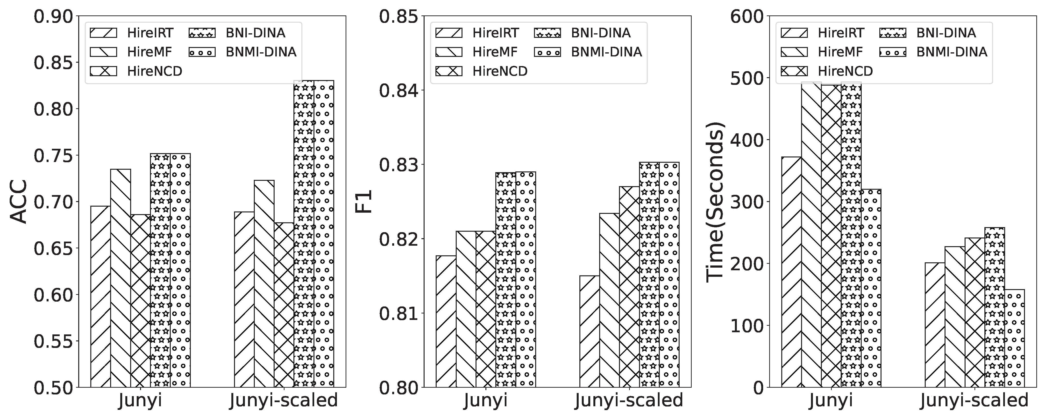
The accuracy of BNMI-DINA significantly outperforms other traditional cognitive diagnosis models. On the Junyi dataset, BNMI-DINA enhances model accuracy by an average of 5.72%. This gap becomes even more obvious on the Junyi-scaled dataset with an improvement of the accuracy by up to 9.21%.
2.
BNMI-DINA has proven to be more computationally efficient than other baselines. The training time is reduced by 26.3% on average while achieving comparable model accuracy.
This observation validates the rationale behind incorporating Bayesian networks for several reasons: (a) Bayesian networks are constructed based on probabilistic graphical models, allowing them to handle the inherent uncertainty in the data. (b) Bayesian networks enable the modeling of interdependencies between variables, providing a better understanding of the data structure and an accurate representation of the relationships between variables. This capability holds true even when working with small datasets.
We also include the comparison results of BNMI-DINA, BNI-DINA (the non-parallel version of BNMI-DINA), and other baseline algorithms in Figure 4 and Figure 5. Our observations from these figures confirm that BNMI-DINA consistently outperforms the other algorithms in all evaluation metrics, regardless of whether they incorporate Bayesian networks or not, and regardless of the dataset used. Additionally, we note that the computation efficiency of the Bayesian network-integrated I-DINA initially appears lower without parallel processing. However, when parallel processing is incorporated, the model demonstrates significantly improved efficiency while maintaining similar levels of accuracy and F1 scores. The reasons are multi-fold:
  • Improvement in estimation process: MI-DINA breaks down the estimation process into smaller subtasks and runs them in parallel. The main process then combines the results, which speeds up the overall diagnostic process. This improvement enhances the efficiency and effectiveness of the model.
  • Enhancements in E-step and M-step: the MI-DINA model enhances the E-step and M-step without affecting the convergence of parameters. Key parameter estimation can still occur iteratively. This enhancement ensures that the estimation process is accurate and reliable.
  • Fusion of Bayesian networks: incorporating Bayesian networks in the approach focuses on estimating students’ mastery probabilities for each knowledge point. This allows for the capture of complex dependencies between variables in cognitive diagnosis, resulting in more accurate understanding of the relationships between students’ cognition and knowledge attributes.

7. Conclusions

In this work, we proposed a novel approach called BNMI-DINA, which is a parallelized incremental DINA model integrated with Bayesian networks. Our proposed model leverages Bayesian networks to establish the dependency relationships between knowledge points. By calculating the posterior probabilities of each node based on the mastery levels of its parent nodes, we obtain an estimation vector that represents students’ mastery levels. Subsequently, we apply the MI-DINA framework, utilizing the students’ response matrix, to estimate the final mastery level estimation matrix. This combined approach significantly enhances both the accuracy and computational speed of the DINA model. Furthermore, we provided theoretical guarantees for the effectiveness of our model. To validate the efficacy of our proposed model, we conducted experiments using real-world datasets. The experimental results demonstrate the superior performance and utility of BNMI-DINA in cognitive diagnosis tasks. In our future work, we plan to explore the extension of BNMI-DINA to adapt to dynamic and adaptive testing scenarios, so as to better improve the accuracy of cognitive diagnosis models in scenarios with a large number of users and rich inspection knowledge points.

Author Contributions

Conceptualization, Y.C. and S.L.; Methodology, Y.C. and S.L.; Validation, Y.C.; Investigation, Y.C. and S.L.; Data curation, Y.C.; Writing original draft preparation: Y.C. and S.L.; Writing review and editing: Y.C. and S.L.; Project administration, Y.C. All authors have read and agreed to the published version of the manuscript.

Funding

This research received no external funding.

Data Availability Statement

Conflicts of Interest

The authors declare no conflict of interest.

References

  1. Templin, J.L.; Henson, R.A. Measurement of psychological disorders using cognitive diagnosis models. Psychol. Methods 2006, 11, 287. [Google Scholar] [CrossRef] [PubMed]
  2. Wang, F.; Huang, Z.; Liu, Q.; Chen, E.; Yin, Y.; Ma, J.; Wang, S. Dynamic Cognitive Diagnosis: An Educational Priors-Enhanced Deep Knowledge Tracing Perspective. IEEE Trans. Learn. Technol. 2023, 16, 306–323. [Google Scholar] [CrossRef]
  3. Liu, Y.; Zhang, T.; Wang, X.; Yu, G.; Li, T. New development of cognitive diagnosis models. Front. Comput. Sci. 2023, 17, 171604. [Google Scholar] [CrossRef]
  4. Luo, J.; Hubaux, J.P. A survey of research in inter-vehicle communications. In Embedded Security in Cars: Securing Current and Future Automotive IT Applications; Springer: Berlin/Heidelberg, Germany, 2006; pp. 111–122. [Google Scholar]
  5. De La Torre, J. DINA model and parameter estimation: A didactic. J. Educ. Behav. Stat. 2009, 34, 115–130. [Google Scholar] [CrossRef]
  6. Wafa, M.N.; Zia, Z.; Frozan, F. Consistency and Ability of Students Using DINA and DINO Models. Eur. J. Math. Stat. 2023, 4, 7–13. [Google Scholar] [CrossRef]
  7. Frederiksen, N.; Mislevy, R.J.; Bejar, I.I. Test Theory for a New Generation of Tests; Routledge: London, UK, 2012. [Google Scholar]
  8. Nichols, P.D.; Chipman, S.F.; Brennan, R.L. Cognitively Diagnostic Assessment; Routledge: London, UK, 2012. [Google Scholar]
  9. Leighton, J.; Gierl, M. Cognitive Diagnostic Assessment for Education: Theory and Applications; Cambridge University Press: Cambridge, UK, 2007. [Google Scholar]
  10. Lee, Y.W.; Sawaki, Y. Cognitive diagnosis approaches to language assessment: An overview. Lang. Assess. Q. 2009, 6, 172–189. [Google Scholar] [CrossRef]
  11. Gu, Z. Maximizing the Potential of Multiple-Choice Items for Cognitive Diagnostic Assessment; University of Toronto Canada: Toronto, ON, Canada, 2011. [Google Scholar]
  12. Li, H.; Hunter, C.V.; Lei, P.W. The selection of cognitive diagnostic models for a reading comprehension test. Lang. Test. 2016, 33, 391–409. [Google Scholar] [CrossRef]
  13. Yang, Y. Modeling Nonignorable Missingness with Response Times Using Tree-Based Framework in Cognitive Diagnostic Models; Columbia University: New York, NY, USA, 2023. [Google Scholar]
  14. Yang, S.; Wei, H.; Ma, H.; Tian, Y.; Zhang, X.; Cao, Y.; Jin, Y. Cognitive diagnosis-based personalized exercise group assembly via a multi-objective evolutionary algorithm. IEEE Trans. Emerg. Top. Comput. Intell. 2023, 7, 829–844. [Google Scholar] [CrossRef]
  15. Qi, T.; Ren, M.; Guo, L.; Li, X.; Li, J.; Zhang, L. ICD: A new interpretable cognitive diagnosis model for intelligent tutor systems. Expert Syst. Appl. 2023, 215, 119309. [Google Scholar] [CrossRef]
  16. Ma, H.; Huang, Z.; Tang, W.; Zhu, H.; Zhang, H.; Li, J. Predicting Student Performance in Future Exams via Neutrosophic Cognitive Diagnosis in Personalized E-learning Environment. IEEE Trans. Learn. Technol. 2023, 16, 680–693. [Google Scholar] [CrossRef]
  17. Gao, W.; Wang, H.; Liu, Q.; Wang, F.; Lin, X.; Yue, L.; Zhang, Z.; Lv, R.; Wang, S. Leveraging Transferable Knowledge Concept Graph Embedding for Cold-Start Cognitive Diagnosis. In Proceedings of the 46th International ACM SIGIR Conference on Research and Development in Information Retrieval, Taipei, Taiwan, 23–27 July 2023; pp. 983–992. [Google Scholar]
  18. Wang, S.; Zeng, Z.; Yang, X.; Zhang, X. Self-supervised graph learning for long-tailed cognitive diagnosis. In Proceedings of the AAAI Conference on Artificial Intelligence, Washington, DC, USA, 7–14 February 2023; Volume 37, pp. 110–118. [Google Scholar]
  19. Wu, R.; Liu, Q.; Liu, Y.; Chen, E.; Su, Y.; Chen, Z.; Hu, G. Cognitive modelling for predicting examinee performance. In Proceedings of the Twenty-Fourth International Joint Conference on Artificial Intelligence, Buenos Aires, Argentina, 25–31 July 2015. [Google Scholar]
  20. De La Torre, J.; Douglas, J.A. Higher-order latent trait models for cognitive diagnosis. Psychometrika 2004, 69, 333–353. [Google Scholar] [CrossRef]
  21. Tu, D.B.; Cai, Y.; Dai Hai-Qi, D. A polytomous cognitive diagnosis model: P-DINA model. Acta Psychol. Sin. 2010, 42, 1011. [Google Scholar] [CrossRef]
  22. Aryadoust, V. A cognitive diagnostic assessment study of the listening test of the Singapore–Cambridge general certificate of education O-level: Application of DINA, DINO, G-DINA, HO-DINA, and RRUM. Int. J. List. 2021, 35, 29–52. [Google Scholar] [CrossRef]
  23. Wang, C.; Liu, Q.; Chen, E.H.; Huang, Z.Y.; Zhu, T.Y.; Su, Y.; Hu, G.P. The rapid calculation method of DINA model for large scale cognitive diagnosis. Acta Electonica Sin. 2018, 46, 1047. [Google Scholar]
  24. Pearl, J. Probabilistic Reasoning in Intelligent Systems: Networks of Plausible Inference; Morgan Kaufmann: Burlington, MA, USA, 1988. [Google Scholar]
  25. Murphy, K.P. Inference and Learning in Hybrid Bayesian Networks; Citeseer: Berkeley, CA, USA, 1998. [Google Scholar]
  26. Tang, J.; Liu, X.; Wang, W. COVID-19 medical waste transportation risk evaluation integrating type-2 fuzzy total interpretive structural modeling and Bayesian network. Expert Syst. Appl. 2023, 213, 118885. [Google Scholar] [CrossRef] [PubMed]
  27. Chan, L.S.; Chu, A.M.; So, M.K. A moving-window bayesian network model for assessing systemic risk in financial markets. PLoS ONE 2023, 18, e0279888. [Google Scholar] [CrossRef] [PubMed]
  28. Kamil, M.Z.; Taleb-Berrouane, M.; Khan, F.; Amyotte, P.; Ahmed, S. Textual data transformations using natural language processing for risk assessment. Risk Anal. 2023, 43, 2033–2052. [Google Scholar] [CrossRef]
  29. Yang, H.; Qi, T.; Li, J.; Guo, L.; Ren, M.; Zhang, L.; Wang, X. A novel quantitative relationship neural network for explainable cognitive diagnosis model. Knowl. Based Syst. 2022, 250, 109156. [Google Scholar] [CrossRef]
  30. Conati, C.; Gertner, A.; Vanlehn, K. Using Bayesian networks to manage uncertainty in student modeling. User Model. User Adapt. Interact. 2002, 12, 371–417. [Google Scholar] [CrossRef]
  31. VanLehn, K.; Lynch, C.; Schulze, K.; Shapiro, J.A.; Shelby, R.; Taylor, L.; Treacy, D.; Weinstein, A.; Wintersgill, M. The Andes physics tutoring system: Lessons learned. Int. J. Artif. Intell. Educ. 2005, 15, 147–204. [Google Scholar]
  32. Käser, T.; Klingler, S.; Schwing, A.G.; Gross, M. Beyond knowledge tracing: Modeling skill topologies with bayesian networks. In Proceedings of the Intelligent Tutoring Systems: 12th International Conference, ITS 2014, Honolulu, HI, USA, 5–9 June 2014; Springer: Berlin/Heidelberg, Germany, 2014; pp. 188–198. [Google Scholar]
  33. Pelánek, R. Bayesian knowledge tracing, logistic models, and beyond: An overview of learner modeling techniques. User Model. User Adapt. Interact. 2017, 27, 313–350. [Google Scholar] [CrossRef]
  34. Liu, S.; Qu, H.; Chen, Q.; Jian, W.; Liu, R.; You, L. AFMeta: Asynchronous Federated Meta-learning with Temporally Weighted Aggregation. In Proceedings of the 2022 IEEE Smartworld, Ubiquitous Intelligence & Computing, Scalable Computing & Communications, Digital Twin, Privacy Computing, Metaverse, Autonomous & Trusted Vehicles (SmartWorld/UIC/ScalCom/DigitalTwin/PriComp/Meta), Haikou, China, 15–18 December 2022; IEEE: Piscataway, NJ, USA, 2022; pp. 641–648. [Google Scholar]
  35. Liu, S.; He, T.; Li, J.; Li, Y.; Kumar, A. An effective learning evaluation method based on text data with real-time attribution-a case study for mathematical class with students of junior middle school in China. ACM Trans. Asian Low Resour. Lang. Inf. Process. 2023, 22, 1–22. [Google Scholar] [CrossRef]
  36. Liu, S.; Yu, X.; Ma, H.; Wang, Z.; Qin, C.; Zhang, X. Homogeneous Cohort-Aware Group Cognitive Diagnosis: A Multi-grained Modeling Perspective. In Proceedings of the 32nd ACM International Conference on Information and Knowledge Management, Birmingham, UK, 21–25 October 2023; pp. 4094–4098. [Google Scholar]
  37. Zhang, S.; Huang, S.; Yu, X.; Chen, E.; Wang, F.; Huang, Z. A generalized multi-skill aggregation method for cognitive diagnosis. World Wide Web 2023, 26, 585–614. [Google Scholar] [CrossRef] [PubMed]
  38. Zhang, Z.; Zhang, J.; Lu, J.; Tao, J. Bayesian estimation of the dina model with Pólya-gamma Gibbs sampling. Front. Psychol. 2020, 11, 384. [Google Scholar] [CrossRef] [PubMed]
  39. Bi, H.; Chen, E.; He, W.; Wu, H.; Zhao, W.; Wang, S.; Wu, J. BETA-CD: A Bayesian meta-learned cognitive diagnosis framework for personalized learning. In Proceedings of the AAAI Conference on Artificial Intelligence, Washington, DC, USA, 7–14 February 2023; Volume 37, pp. 5018–5026. [Google Scholar]
  40. McLachlan, G. On Aitken’s method and other approaches for accelerating convergence of the EM algorithm. In Proceedings of the AC Aitken Centenary Conference, Dunedin, New Zealand, 28 August–1 September 1995; pp. 201–209. [Google Scholar]
  41. Dempster, A.P.; Laird, N.M.; Rubin, D.B. Maximum likelihood from incomplete data via the EM algorithm. J. R. Stat. Soc. Ser. B (Methodol.) 1977, 39, 1–22. [Google Scholar] [CrossRef]
  42. Geiger, D.; Pearl, J. Logical and algorithmic properties of independence and their application to Bayesian networks. Ann. Math. Artif. Intell. 1990, 2, 165–178. [Google Scholar] [CrossRef]
  43. Thiesson, B.; Meek, C.; Heckerman, D. Accelerating EM for large databases. Mach. Learn. 2001, 45, 279–299. [Google Scholar] [CrossRef]
  44. Chang, H.S.; Hsu, H.J.; Chen, K.T. Modeling Exercise Relationships in E-Learning: A Unified Approach. In Proceedings of the EDM, Madrid, Spain, 26–29 June 2015; pp. 532–535. [Google Scholar]
  45. Hadi, M.A.; Fard, F.H. Evaluating pre-trained models for user feedback analysis in software engineering: A study on classification of app-reviews. Empir. Softw. Eng. 2023, 28, 88. [Google Scholar] [CrossRef]
  46. Koren, Y.; Bell, R.; Volinsky, C. Matrix factorization techniques for recommender systems. Computer 2009, 42, 30–37. [Google Scholar] [CrossRef]
  47. Wang, F.; Liu, Q.; Chen, E.; Huang, Z.; Yin, Y.; Wang, S.; Su, Y. NeuralCD: A general framework for cognitive diagnosis. IEEE Trans. Knowl. Data Eng. 2022, 35, 8312–8327. [Google Scholar] [CrossRef]
  48. Li, J.; Wang, F.; Liu, Q.; Zhu, M.; Huang, W.; Huang, Z.; Chen, E.; Su, Y.; Wang, S. HierCDF: A Bayesian Network-based Hierarchical Cognitive Diagnosis Framework. In Proceedings of the 28th ACM SIGKDD Conference on Knowledge Discovery and Data Mining, Washington, DC, USA, 14–18 August 2022; pp. 904–913. [Google Scholar]
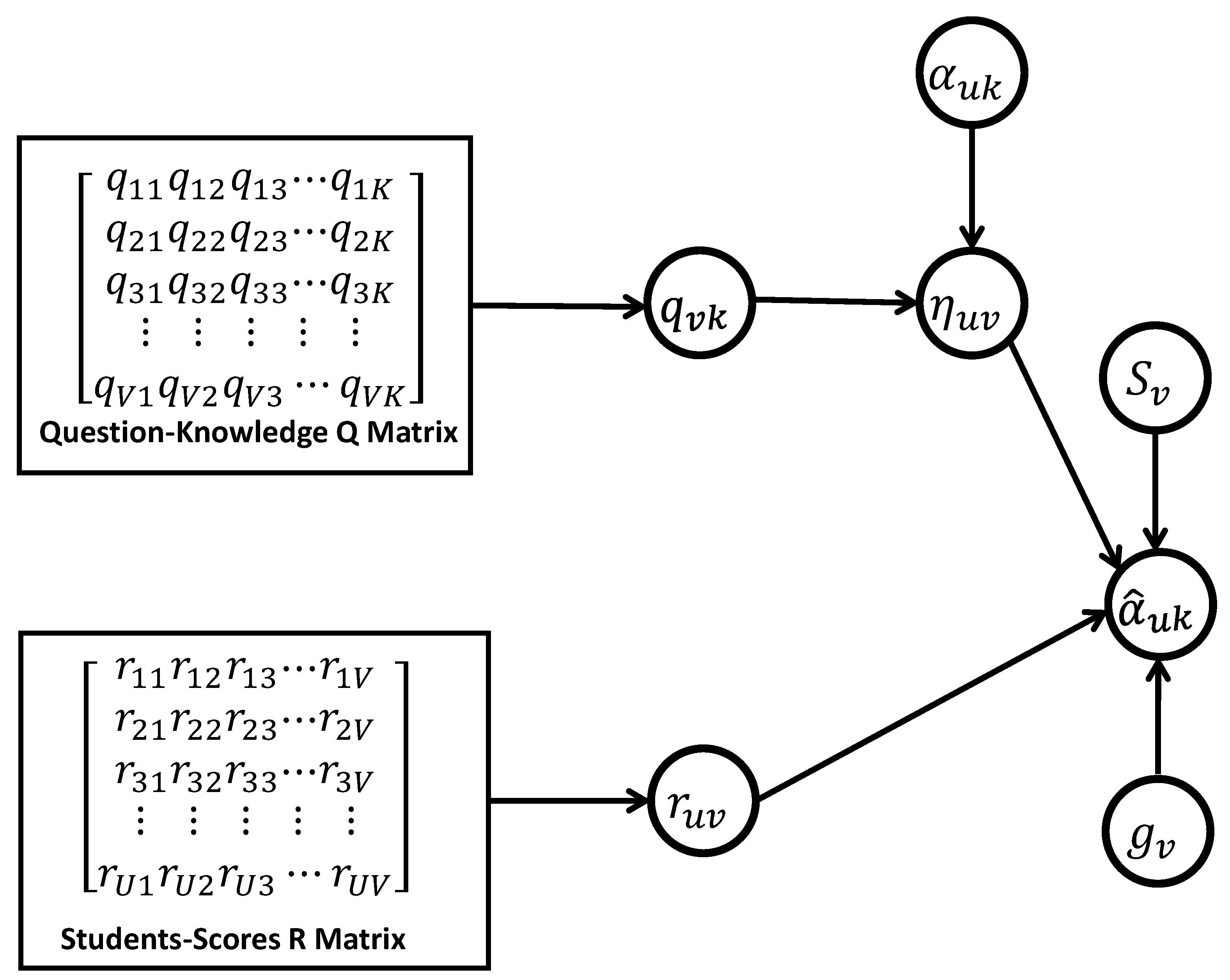
Figure 1. An overview of the DINA model. The rectangle represents the matrix, the circle represents a variable and the arrow refers to the computational dependencies between different variables.
Bdcc 08 00004 g001
Figure 2. The framework of BNMI-DINA. Nodes a–e represent knowledge points.
Bdcc 08 00004 g002
Figure 3. Examples of hierarchical relationship between knowledge points on Junyi dataset. (a) Junyi dataset visual knowledge point attribute relationship. (b) Correspondence between nodes and knowledge points.
Bdcc 08 00004 g003
Figure 4. Comparison results of BNMI-DINA and BNI-DINA with other baseline models that do not incorporate Bayesian networks.
Bdcc 08 00004 g004
Figure 5. Comparison results of BNMI-DINA and BNI-DINA with other baseline models that incorporate Bayesian networks.
Bdcc 08 00004 g005
Table 1. Overview of key aspects of related work.
AspectSummary
Cognitive DiagnosisOver 60 cognitive diagnosis models have been developed, including the rule-based model, attribute hierarchy model, DINA model, and various variations such as the Fuzzy CDF model.
Bayesian NetworksBayesian Networks were introduced in 1988 and further expanded in the 1990s, leading to their widespread application in various domains.
DINA ModelThe DINA model has recently been a focus of exploration in education for student modeling, knowledge tracing, and skill topology.
Our WorkOur work not only incorporates a Bayesian network to capture the dependency relationship between knowledge points, but also enhances computational efficiency, particularly for large datasets.
Table 2. Summary of major notations.
SymbolDescription
QQuestion-Knowledge point matrix
RStudent-Question score matrix
USet of student blocks
iStudent number
R i Question score of student i
R a Computed question scores of student block U a
z l ( α l ) Probability mass function (joint probability distribution function)
oInitial knowledge point mastery probability
γ Posterior probability of knowledge point mastery
η Hidden mastery status matrix
rStudent’s score
kSub-knowledge point
KTotal number of knowledge points
xParent knowledge point
uStudent user
tIteration number
lCombination of knowledge point mastery
DNumber of combinations of knowledge point mastery
α Matrix of knowledge point mastery for all students
α u Matrix of knowledge point mastery for student user u
α l Matrix of knowledge point mastery for combination l
α ^ Estimated matrix of knowledge point mastery for student
sSlip parameter
gGuess parameter
vQuestion
VTotal number of questions
nNumber of parent knowledge points
NTotal number of student blocks
Table 3. The statistics of datasets.
Dataset#Students#Attributes#Question Items#Response Logs
Junyi10,000734734408,057
Junyi-scaled240010106100
Table 4. Experimental results on student performance prediction.
DatasetsMetricsIRTMFNeural CDDINA
OriginalHierOriginalHierOriginalHierBNI-DINABNMI-DINA
JunyiACC0.72180.69510.72210.73480.68210.68600.75160.7517
F10.81250.81770.81430.82100.82140.82100.82890.8290
Time366372478493479488493320
Junyi-scaledACC0.68740.68890.70440.72280.65170.67710.75030.7503
F10.80790.81500.81710.82340.82660.82700.83030.8303
Time174201213227229241258158
Disclaimer/Publisher’s Note: The statements, opinions and data contained in all publications are solely those of the individual author(s) and contributor(s) and not of MDPI and/or the editor(s). MDPI and/or the editor(s) disclaim responsibility for any injury to people or property resulting from any ideas, methods, instructions or products referred to in the content.