Article

Detecting Multi-Density Urban Hotspots in a Smart City: Approaches, Challenges and Applications

1
DiCES Department, University of Calabria, Via Pietro Bucci 18B, 87036 Rende, CS, Italy
2
DIMES Department, University of Calabria, Via Pietro Bucci 42c, 87036 Rende, CS, Italy
3
Institute for High-Performance Computing and Networking (ICAR), CNR—National Research Council of Italy, Via Pietro Bucci, Cubo 8/9C, 87036 Rende, CS, Italy
*
Author to whom correspondence should be addressed.
These authors contributed equally to this work.
Big Data Cogn. Comput. 2023, 7(1), 29; https://doi.org/10.3390/bdcc7010029
Submission received: 28 December 2022 / Revised: 22 January 2023 / Accepted: 3 February 2023 / Published: 8 February 2023

Abstract

:
Leveraged by a large-scale diffusion of sensing networks and scanning devices in modern cities, huge volumes of geo-referenced urban data are collected every day. Such an amount of information is analyzed to discover data-driven models, which can be exploited to tackle the major issues that cities face, including air pollution, virus diffusion, human mobility, crime forecasting, traffic flows, etc. In particular, the detection of city hotspots is de facto a valuable organization technique for framing detailed knowledge of a metropolitan area, providing high-level summaries for spatial datasets, which are a valuable support for planners, scientists, and policymakers. However, while classic density-based clustering algorithms show to be suitable for discovering hotspots characterized by homogeneous density, their application on multi-density data can produce inaccurate results. In fact, a proper threshold setting is very difficult when clusters in different regions have considerably different densities, or clusters with different density levels are nested. For such a reason, since metropolitan cities are heavily characterized by variable densities, multi-density clustering seems to be more appropriate for discovering city hotspots. Indeed, such algorithms rely on multiple minimum threshold values and are able to detect multiple pattern distributions of different densities, aiming at distinguishing between several density regions, which may or may not be nested and are generally of a non-convex shape. This paper discusses the research issues and challenges for analyzing urban data, aimed at discovering multi-density hotspots in urban areas. In particular, the study compares the four approaches (DBSCAN, OPTICS-xi, HDBSCAN, and CHD) proposed in the literature for clustering urban data and analyzes their performance on both state-of-the-art and real-world datasets. Experimental results show that multi-density clustering algorithms generally achieve better results on urban data than classic density-based algorithms.

1. Introduction

Reference Context. Cities worldwide are experiencing significant evolution due to numerous factors, e.g., new forms of communication, new ways of transportation, and fast urbanization. The pervasive and large-scale diffusion of sensing networks, image-scanning devices, and GPS devices is enabling the collection of huge volumes of geo-referenced urban data every day. As more and more data become available, data scientists can analyze such an abundance of urban spatial data to discover predictive and descriptive data-driven models, which can assist city managers in dealing with the major problems that cities face, e.g., human mobility, traffic flows, air pollution, crime forecasts, and virus diffusion [1,2,3,4,5,6,7,8,9]. In particular, detecting city hotspots is emerging as a frequent task when analyzing urban data. In fact, given the availability of geo-referenced data, it is useful to detect areas where urban events (e.g., crimes, traffic spikes, viral infections, and pollution peaks) occur with a higher density than in other regions of the dataset. Additionally, hotspot detection can serve as a useful organizational technique for elaborating thorough knowledge of an urban area, and their borders and shapes can enable high-level spatial knowledge summaries, which are valuable for policymakers, scientists, and planners [5,10,11]. As an instance, environmental scientists are interested in partitioning a city into uniform regions based on environmental characteristics and pollution density [3,12]. Similarly, during viral emergencies, as recently happened with the COVID-19 pandemic, virologists and epidemiologists are steadily interested in detecting city hotspots in which viruses are spreading with higher densities than other areas of the same city [6,7,13]. Moreover, city administrators can be interested in determining uniform regions of a city with respect to the functions they serve for citizens or visiting people. Additionally, police authorities are interested in detecting crime hotspots (i.e., areas with a high crime density) to ensure public safety in the city territory better [4,5]. Regarding data analysis, the search for intra-hotspot and inter-hotspot models is a hot topic for scientists. For instance, intra-hotspot models can reveal the changes in density within a hotspot over time, and inter-hotspot models can study how the appearance of a given hotspot can affect the generation of other hotspots in a different area  [14].
Motivations. In metropolitan cities, the density of events, traffic, or population can differ widely between different areas, making urban regions highly dissimilar regarding density. This issue is made evident in Figure 1, which shows how inter-city and intra-city population densities strongly differ in different metropolitan city areas. Specifically, Figure 1a plots the population density of the 200 densest square kilometer grid cells in six representative cities [15], while the coefficient of variation of the population density of several countries is shown in Figure 1b. Focusing on the first chart (https://garrettdashnelson.github.io/square-density/, accessed on 18 December 2022), we can observe that densities largely vary within the same city, and between several cities. As an instance, New York City represents a classic case of multi-density regions: there are several high-density areas (Manhattan), and many other low-density areas (Queens). Chicago shows similarly top-heavy density pyramids, where the high-density areas (Loop and Near North Side) stand out from the rest of the region [15]. Other cities, such as Boston, San Francisco, and Los Angeles, show similarly multi-density distributions, with a high variation of densities among different city regions. As a second observation, it is worth noting that densities largely vary between several cities. For example, it is worth noting that the lowest-density areas of New York City are even denser than the densest parts of Dallas or Boston, and that even Chicago and Los Angeles’ densest areas barely crack into the bottom half of New York City’s top 200. On the other side, Figure 1b shows the average, minimum, and maximum values (and the names of the corresponding cities) of the coefficient of variation of the population density for several countries [16]. The coefficient of variation displayed in Figure 1b is defined as the relative standard deviation of urban population density, i.e.,  C V = S D / P D , where given a city, S D is the standard deviation of population density within the city, and  P D is the average population density of the same area. Thus, the coefficient of variation is a unit-free measure of the density variation of the population within a city. The higher the coefficient of density variation of a city, the higher the dispersion in the population density of a city. The chart confirms a very high variability of densities within the same country, and between several countries. For example, in Mexico, the coefficient of variation ranges from 1.05 in Mexico City to 14.03 in Navajoa, showing an extremely high dispersion in population density. A similar observation can be made for Korea, the U.S., Canada, and the other listed countries. This aspect must be taken in consideration to properly infer the real hotspots when analyzing urban data. The density of traffic, events, population, etc., in metropolitan cities can largely differ between different areas, making urban regions extremely dissimilar in terms of density. It is worth noting that, in our experience, given an urban area and a set of events (related to, for example, crimes, COVID infections, and mobility), high-density variations can be observed in the collected data.
Clustering is the most appropriate technique to discover urban hotspots. However, we can split such algorithms into two groups. The first group includes algorithms that, due to the adoption of global parameters, define a single minimum threshold value to distinguish between dense and not-dense areas. Often, a proper threshold setting becomes all the more difficult when clusters in different regions of the feature space have considerably different densities, or clusters with different density levels are nested. In such cases, the partitioning might not be proper with one single-density threshold. In fact, if the chosen threshold is too high, they can discover several small non-significant clusters that actually do not represent dense regions; otherwise, if the chosen threshold is too low, they can discover a few large regions that actually are no longer dense as well. As a matter of fact, the application of such algorithms to a multi-density dataset, such as urban data, could not achieve good results. The second group includes algorithms that rely on multiple minimum threshold values. Such algorithms generally detect multiple pattern distributions of different densities, aiming at distinguishing between several density regions, which may or may not be nested and are generally of a non-convex shape. Then, they automatically estimate the number of threshold values to optimally identify the different density regions, without any prior knowledge about the data. Such algorithms usually detect better data partitioning than single-density threshold algorithms, but their drawback is a very high computational cost.
Contributions and plan of the paper. Given the presented context, this paper presents a study on hotspots detection in urban environments. As the main contribution, the study compares the most important approaches proposed in the literature for clustering urban data and analyzes their results on two synthetic datasets and a real-world one, having in mind two different goals. The experimental evaluation on synthetic state-of-the-art multi-density datasets is performed to evaluate the clustering quality and the ability of the algorithms to retrieve proper hotspots. To do that, we exploit two synthetic datasets, where each point owns a target cluster label, and thus the algorithms could be evaluated qualitatively and quantitatively by taking advantage of such ground truth information. The experimental evaluation on real-world data is performed on crime data from the Chicago Police Department, inherently characterized by points distributed with very different densities in the city area. Such a concrete scenario is exploited to show the practical usefulness of density-based clustering algorithms in discovering multi-density urban hotspots in real urban cases.
The remainder of the paper is structured as follows. Section 2 briefly describes the most important density-based approaches in spatial clustering literature, and the most representative projects in that field of research. Section 3 presents a selection of the main density-based clustering algorithms exploited in the literature to analyze urban data, by summarizing how they work. Section 4 provides the comparative experimental evaluation of the different approaches on state-of-the-art datasets. Section 5 shows the algorithm results on a real-world scenario. Finally, Section 6 concludes the paper and plans future research works.

2. Related Works

The analysis of urban data and the detection of urban hotspots from geo-referenced data are very challenging tasks. For this purpose, several approaches have been proposed in the literature, tackling the problem by adopting clustering approaches. In some cases, the discovery of urban hotspots represents one step of a more complex workflow, based on a common inspiring idea of several approaches that first detect geographic hotspots and then extract predictive models of intra-hotspots and/or inter-hotspots. In this section, we briefly review the most representative research work in the area.
The DSPM (density-based sequential pattern mining) approach, aimed at the discovery of mobility patterns from GPS data, is proposed in [2]. The method consists of (i) discovering urban dense regions of interest (more densely passed through ones) and (ii) extracting mobility patterns among those regions. As a case study, the approach is applied to a real-life GPS dataset tracing the movement of taxis in the urban area of Beijing. Additionally, the authors describe a comprehensive validation methodology for assessing the accuracy and quality of detected dense regions and trajectory patterns. The approach relies on the DBSCAN algorithm for detecting dense regions and could be improved by considering multi-density clustering analysis, detecting also lower-dense but homogeneous regions.
An approach to predict ozone concentrations at given target observation stations, based on spatial clustering and multilayer perceptron models, is proposed [18]. In particular, the approach exploits k-means clustering to detect similar stations and then train them together to get a base model for spatial transfer learning. The final models are used to predict the ozone concentration for three-day-ahead prediction horizons. The experimental evaluation, performed using historical data of stations in Germany, has shown higher forecasting accuracy of ozone exceedances with respect to traditional chemical transport models and popular machine learning approaches. Since the work groups sensor stations which are localized on a large area, it could benefit from exploiting multi-density clustering algorithms instead of k-means. Additionally, in a recent paper [19], the application of artificial intelligence (AI) and machine learning (ML) to build air pollution models, aimed at forecasting pollutant concentrations and health risks, is analyzed. The paper depicts how air pollution data can be uploaded into AI-ML models to discover the correlation between exposure to pollution and public health risks, giving a survey of applications and challenges of such a research field. In particular, it is pointed out that explainability is one of the paramount requirements in choosing AI-ML models for analyzing pollution data.
In [20], an approach is proposed to predict high-resolution electric consumption trends at finely resolved spatial and temporal scales. The approach is composed of two steps. First, apartment-level historical electric consumptions data are collected and clustered. Second, the clusters are aggregated based on the consumption profiles of consumers. The clustering analysis is performed by the k-means algorithm, while forecasting models are discovered by two deep learning techniques: long short-term memory unit (LSTM) and gated recurrent unit (GRU). The experimental evaluation was performed on electricity consumption data collected from residential buildings situated in an urban area of South Korea. In particular, a comparative analysis with state-of-the-art machine learning models and deep learning variants showed good performance in terms of building- and floor-level prediction accuracy. The clustering of the consumption profiles of the consumers does not take into account features related to the location of apartments, buildings and floors. A multi-density hotspot detection can benefit the analysis, as it could group together building in the same city area, maybe constructed in the same years and having similar characteristics.
In [21], the authors designed a workflow composed of five steps, i.e., data pre-processing, feature extraction, machine learning training, performance evaluation, and explainable artificial intelligence, to analyze the effects of changes in land cover, such as deforestation or urbanization, on the local climate. In particular, machine learning models have been trained to learn the relation between land cover changes and temperature changes. Then, explainable artificial intelligence has been further exploited to interpret and analyze the impact of different land cover changes on temperature. Additionally, the experimental results have shown that random forest outperformed other machine learning methods (e.g., linear regression) proposed in the literature for discovering the relation of land cover–temperature changes.
A methodology for discovering behavior rules, correlations, and mobility patterns of visitors attending large-scale public events by analyzing social media posts is proposed in [22]. In particular, the authors describe a multi-step approach based on the detection of hotspots of interest (bounded areas) where the public events are held, collection of the geo-tagged items related to the events, gathering of trajectories of users publishing posts concerning such events, and discovery of touristic mobility patterns. The methodology is tested through two case studies: a mobility pattern analysis on Instagram users who visited EXPO 2015, and behavior modeling of geo-tagged tweets posted by users attending the 2014 FIFA World Cup, showing reasonable predictive accuracy.
A system for geo-localized crime data analysis, named CrimeTracer, is proposed in [23]. The approach is based on a probabilistic framework to discover spatial clusters in urban areas, and it is applied for crime event forecasting. In particular, the algorithm partitions the area of interest in activity spaces, which represent hotspots frequented by known offenders to make their criminal activities. On the bases of such knowledge, spatial crime predictions are performed on each activity space. Another approach for spatial data clustering is proposed in [24], which classifies locations as crime hotposts or no crime hotspots by exploiting one-class support vector machines (SVM). Similarly, in [25] an approach based on recurrent neural network models is designed to analyze spatial information and classify grid-cells as hotspot or not-hotspot.
An approach aiming at detecting crime hotspots in cities and forecasting crime trends in each hotspot is described in [5]. The approach leverages auto-regressive forecasting models and spatial cluster analysis to build a specific crime predictor for each hotspot detected during the spatial clustering analysis. The predictors can estimate crime trends in terms of the number of expected future crime events. The approach is assessed on real-world data, consisting of crime events collected in New York City and Chicago, and is demonstrated effective in terms of forecasting accuracy considering different time horizons. The above reviewed works in crimes analysis [5,23,24,25] are not capable of considering automatically detected hotspots characterized by different densities.
A predictive approach based on spatial analysis and regressive models is proposed in [13], aiming at discovering spatio-temporal predictive epidemic patterns from infection and mobility data. The algorithm is composed of several steps, starting from the detection of epidemic hotspots (urban areas where infection events occur more densely with respect to others) and mobility hotspots (urban regions more densely visited by mobility traces), to the discovery of epidemic patterns among epidemic hotspots. The approach finally processes each epidemic hotspot and analyzes the infection data of the epidemic hotspots involved in mobility patterns, then it extracts hotspot-specific epidemic forecasting models. The approach has been validated on real-world data regarding mobility and COVID-19 infections in Chicago. The paper focuses only on high-density hotspots in the given analysis and exploits the DBSCAN algorithm for detecting epidemic hotspots. This work can also benefit from the exploitation of other multi-density-based clustering algorithms.

3. Algorithms to Detect Urban Hotspots

This section shortly describes four density-based clustering methods—CHD, DBSCAN, HDBSCAN and OPTICS-Xi—that we selected from the literature as the most used and interesting approaches to analyze urban data.

3.1. DBSCAN

The DBSCAN (density-based spatial clustering of applications with noise) [26] algorithm is the precursor of all density-based clustering algorithms. It was developed to process large datasets with the inherent presence of noise. DBSCAN is capable of discriminating the noise points of a dataset and can detect clusters of any shape with no previous information about the number of expected clusters. Shortly, DBSCAN leverages the concepts of core points, density-reachability, and density-connectivity. Given two parameters ϵ and m i n P t s , a point is a core point if there are at least m i n P t s points in its neighborhood of radius ϵ ( ϵ -neighborhood). A point p is directly density-reachable from a point q if q is a core point and p is in q’s ϵ -neighborhood. Two points p and q are density-reachable if there exists a chain of directly density-reachable points that connect q and p. Finally, two points p and q are density-connected if there exists a core point o such that p and q are density-reachable from o.
DBSCAN builds a cluster of points by iteratively connecting a couple of points that are density-connected, and all the points that are density-reachable from a point of the cluster are in the same cluster. All points that do not belong to any cluster, and thus are not density-connected to any other point, are considered noise points. The DBSCAN can process a dataset of size n in O ( n l o g n ) time if exploiting a proper indexing structure on the data for executing the search for the ϵ -neighborhood. It is worth noting that, given the definitions above, it is clear that DBSCAN can detect clusters having at least a specific pre-determined density ( m i n P t s π r 2 ), directly determined by the ϵ and m i n P t s parameters. For such a reason, it can fail to detect clusters characterized by different densities.

3.2. OPTICS-xi

The OPTICS-xi [27] algorithm is rooted in the concepts of reachability described for the DBSCAN, but it exploits some derived properties to build an ordered structure for the dataset containing information about every ϵ value in a given range, and it uses this structure to generate a proper clustering. The OPTICS indexing structure is based on the assumption that given a constant m i n _ p t s value, density-based clusters with respect to a higher density (i.e., a lower value for ϵ ) are completely contained in density-connected sets with respect to a lower density (i.e., a higher value for ϵ ). For each point, the structure stores the core distance and the reachability distance. Given a parameter m i n _ p t s , the core distance of a point p is the distance ϵ to its m i n P t s t h nearest neighbor (it is undefined whether p has less than m i n P t s neighbors). The reachability distance of point p with respect to a point o is, intuitively, the smallest distance such that p is directly density-reachable from o if o is a core point. By exploiting these above-introduced concepts, the OPTICS-xi algorithm is capable of generating an indexing structure of the dataset that keeps the cluster hierarchy for a variable neighborhood radius. Now, if a specific value for ϵ is chosen, by exploiting the structure, it is possible to perform a clustering that is very similar to the DBSCAN one. Given the generated values of reachability distance stored in the OPTICS indexing structure, the algorithm first generates the related reachability plot, and then it looks at the steep slopes within the graph to find clusters. The  ξ ( 0 < ξ < 1 ) parameter is exploited to define what counts as a steep slope. The results of the xi clustering extraction method are very sensitive to the tuning of the ξ parameter. The OPTICS-xi time complexity is  O ( n l o g n ) .

3.3. HDBSCAN

The HDBSCAN algorithm [28], based on similar concepts defined for OPTICS, computes a complete clustering hierarchy composed of all possible density-based clusters for a large range of density thresholds. Then, it chooses the clustering model that maximizes the overall stability of the extracted clusters. To build such a hierarchy, the HDBSCAN starts from the concepts of mutual reachability distance between two core points p and q and given a value for a parameter m i n _ p t s . The mutual reachability distance is defined as the minimum ϵ radius such that p and q are mutually density-reachable. Differently from the above introduced reachability distance, the mutual reachability distance is symmetric.
HDBSCAN works as follows. First, it builds the clustering hierarchy by computing a mutual reachability graph, which is a complete graph where each vertex is a data point, and each edge is weighted with the mutual reachability distance of the linked couple of points. Then, a minimum spanning tree is computed on that graph, integrated by adding (for each vertex) a self-edge, weighted by the core-distance of the related data point. The tree is processed by removing the edges in decreasing order with respect to their weight. For each removal, the two involved edges are labeled as roots of a new pair of clusters, or noise if the generated component has not any edge. A variation of the summarized algorithm considers also a given minimum cluster size ( m i n _ c l u s t e r _ s i z e parameter), which avoids the generation of clusters having a size lower than m i n _ c l u s t e r _ s i z e . Given the clustering hierarchy, a clustering is extracted which maximizes the overall stability. The notion of stability is derived from the notion of excess of mass [29]. HDBSCAN is able to compute the clustering hierarchy and extract the clusters in O ( n 2 ) time, which is in some cases infeasible and represents the main drawback with respect to DBSCAN and OPTICS.

3.4. City Hotspot Detector

The city hotspot detector (CHD) algorithm [30] is a multi-density based clustering algorithm that has been purposely designed for processing urban spatial data. The algorithm is composed of several steps, as follows. First, given a fixed m i n _ p t s , the reachability distance for each point is computed and exploited as an estimator of the density of each data point. Then, the points are sorted with respect to their estimated density, and the density variation between each consecutive couple of points in the ordered list is computed. The obtained density variation list is then smoothed by applying a rolling mean operator considering windows of size s. The points are then partitioned into several density level sets, on the basis of the smoothed density variations. Then, a different ϵ value is estimated for each density level set. Finally, each set is analyzed by the DBSCAN algorithm. Specifically, each instance takes in input, a specific ϵ value computed for the analyzed density level set. The set of clusters detected for each partition constitutes the final result of the CHD algorithm. The CHD algorithm runs with O ( n l o g n ) time complexity, where n is the size of the processed dataset. A cluster analysis with the CHD algorithm requires the tuning of more parameters (three) with respect to the previously introduced algorithms.

4. Experimental Evaluation and Results

In this section, we provide a comparative analysis of the four density-based clustering algorithms described in Section 3, namely CHD, DBSCAN, HDBSCAN, and OPTICS-Xi, by assessing the quality of the clusters detected by the algorithms and their ability to process datasets characterized by areas with different densities. The comparison is made on the results gathered by analyzing two datasets provided of the target cluster labels that are considered ground truth during the evaluation process. The experiments were carried out by exploiting the implementations provided by the scikit-learn Python library for DBSCAN and OPTICS-xi, the hdbscan Python library for HDBSCAN, and the R implementation of the CHD algorithm available at gitlab (CHD R-code: https://gitlab.com/chd3/chd-rcode/, accessed on 18 December 2022).

4.1. Data Description

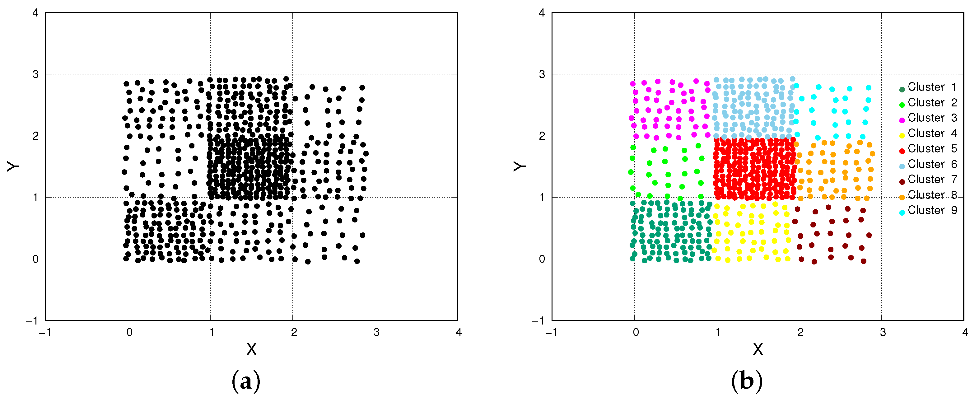
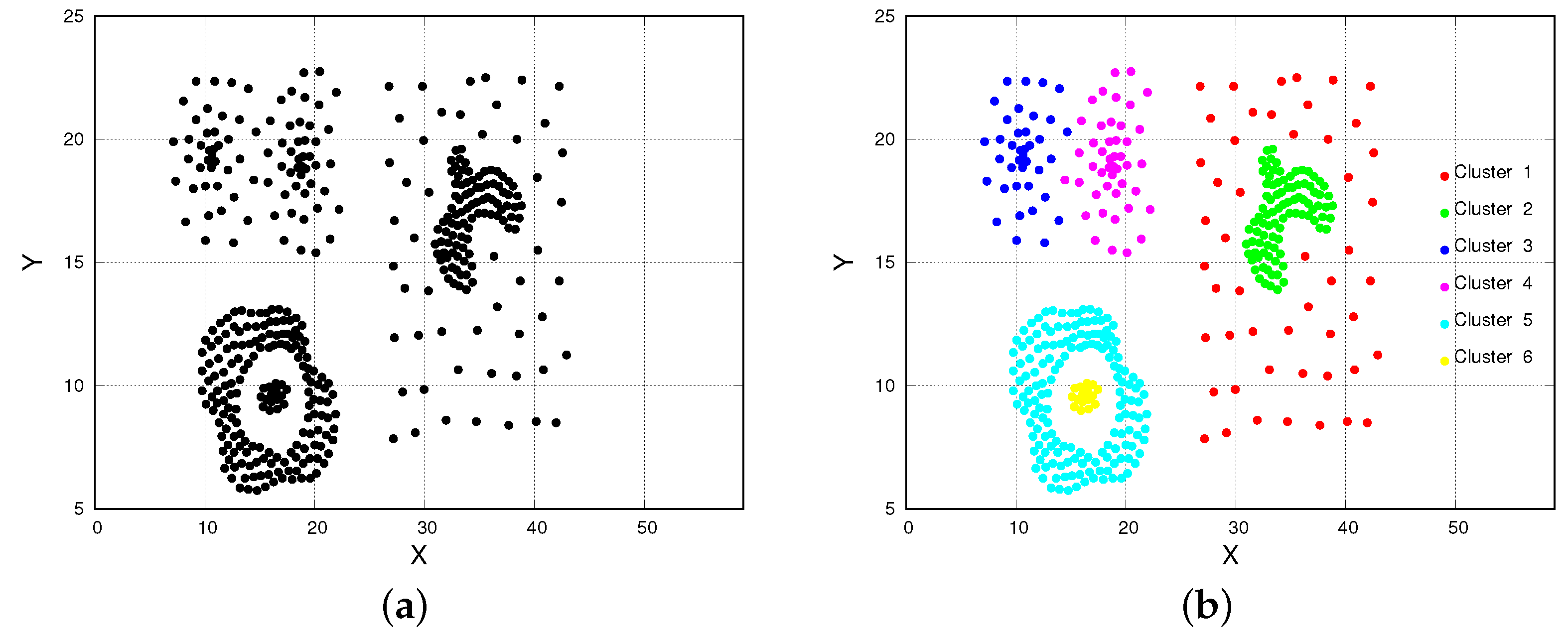
The datasets chosen for the comparative analysis are chess and compound, two cluster-labeled datasets available in the literature [31,32], whose data instances and target clusters are shown in Figure 2 and Figure 3. In particular, the two datasets have different characteristics, as reported in the following:
-
The chess dataset is composed of 618 instances and partitioned in nine target clusters. Each instance is described by X and Y features (Figure 2). Clusters are very contiguous, and they have regular block shapes, different densities and sizes. In particular, the highest density cluster has a density σ 5 C h e s s = 212.54 (cluster n. 5, n. of points = 196, area = 0.92), while the lowest density one has a density σ 7 C h e s s = 31.50 (cluster n. 7, n. of points = 25, area = 0.79).
-
The compound dataset is composed of 399 instances, described by X and Y features, and partitioned in six target clusters (Figure 3). Clusters are well separated, and they have irregular multi-geometric shapes (different from the previous dataset), different densities and sizes. In this dataset, the highest density cluster has a density σ 6 C o m p o u n d = 6.19 (cluster n. 6, n. of points = 16, area = 2.58), while the lowest density cluster has a density σ 1 C o m p o u n d = 0.21 (cluster n. 1, n. of points = 50, area = 236.60).
The multi-density distribution of instances, as well as their multi-shape partitions, makes such datasets very appropriate for our analysis because they model different scenarios to test and validate the algorithms on.

4.2. Results on State-of-the-Art Data

In order to evaluate the performance of the selected clustering algorithms over the above-introduced datasets, we compare the results obtained by the cluster analysis, i.e., the discovered clusters, to the ground truth labels provided by the datasets, i.e., the target clusters. By matching the discovered clusters against the provided target clusters, we can evaluate the effectiveness of the clustering algorithms. To do so, the following set of external metrics, designed to be employed when ground truth labels are available, are here adopted: F o w l k e s , A d j u s t e d R a n d , A d j u s t e d M u t u a l I n f o r m a t i o n ( A M I ) , V- m e a s u r e , A c c u r a c y , F- m e a s u r e , J a c c a r d , Γ , R a n d and H o m o g e n e i t y (more details about such metrics are reported in [33]).
In general, the listed metrics consider the number of items that are incorrectly allocated, i.e., items not assigned to a cluster of points sharing the same target cluster label. According to an external criterion, the result of a clustering algorithm is more satisfactory when fewer items are incorrectly allocated. All the above-listed metrics can assume values in the range [0, 1], where a value of 1 corresponds to a perfect match between discovered and target clusters, and lower values to the presence of a higher number of incorrectly allocated items. Therefore, such external metrics can be exploited to compare the performance results of clustering algorithms according to objective quantitative criteria.
It is worth noting that, for each clustering algorithm, the choice of the input parameters directly impacts the quality of the results; therefore, in order to make a fair comparison between the clustering algorithms, there is the need to carefully pick the input parameters with respect to the analyzed dataset. Let us recall that CHD receives k, ω and s as input parameters; DBSCAN requires the setting of ϵ and m i n _ p t s ; HDBSCAN receives m i n _ c l u s t e r _ s i z e and m i n _ p t s [28] as input parameters; and OPTICS-Xi requires the setting of ξ and m i n _ p t s .
In this paper, we adopted a parameter sweeping methodology for selecting the input parameters. Such a methodology consists in running several instances of each algorithm exploiting different parameter settings. For each algorithm, the parameter settings resulting in the best average performance, computed as the average of the above-listed metrics, are chosen. This process enables the modeler to determine a parameter’s "best" value. Table 1 shows some details about the experimental setting adopted during the parameter sweeping. In particular, for each algorithm, the table reports the fixed parameter values, the chosen parameter to be swept and its range of values, the obtained best parameter value, and the corresponding best average performance.
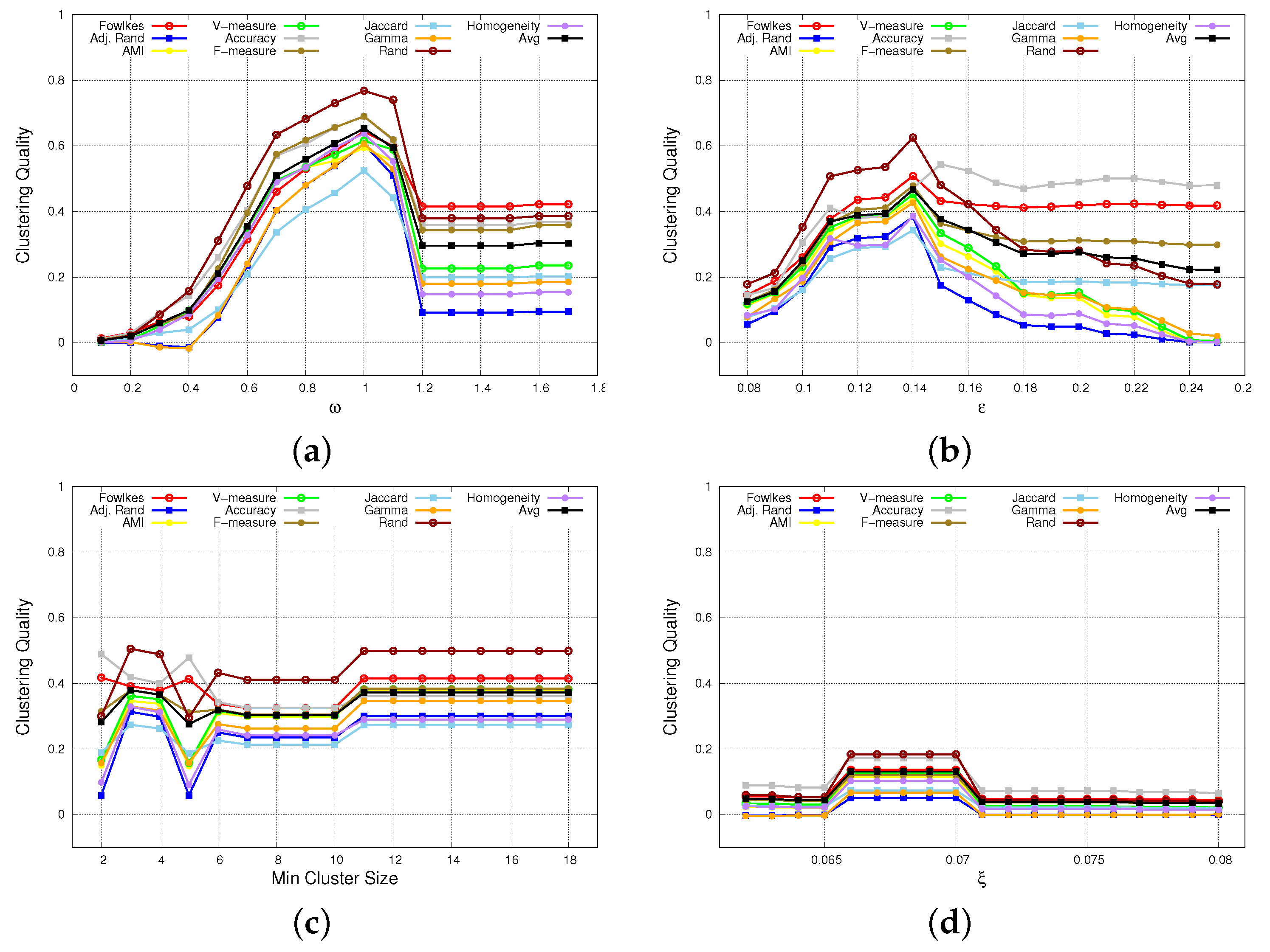
Figure 4 reports the first set of experimental results, obtained on the chess dataset. The figure shows how quality indices vary versus swept input parameter values. Regarding the CHD algorithm (Figure 4a), it is clear how the trend is strongly affected by the values of the ω parameter, and the best results are obtained by considering ω * = 1.00 . The DBSCAN algorithm is evaluated by varying the ϵ parameter from 0.08 to 0.22 ( m i n P t s = 4 ), and the best result is achieved for ϵ * = 0.14 (see Figure 4b). Similarly, we evaluate different input parameters settings for HDBSCAN (Figure 4c) and OPTICS-xi (Figure 4d). Even in these cases, little variations of the input parameters strongly affect the quality of the results. The best results are achieved considering m i n _ c l u s t e r _ s i z e * = 3 for HDBSCAN and ξ * = 0.066 for OPTICS-xi.
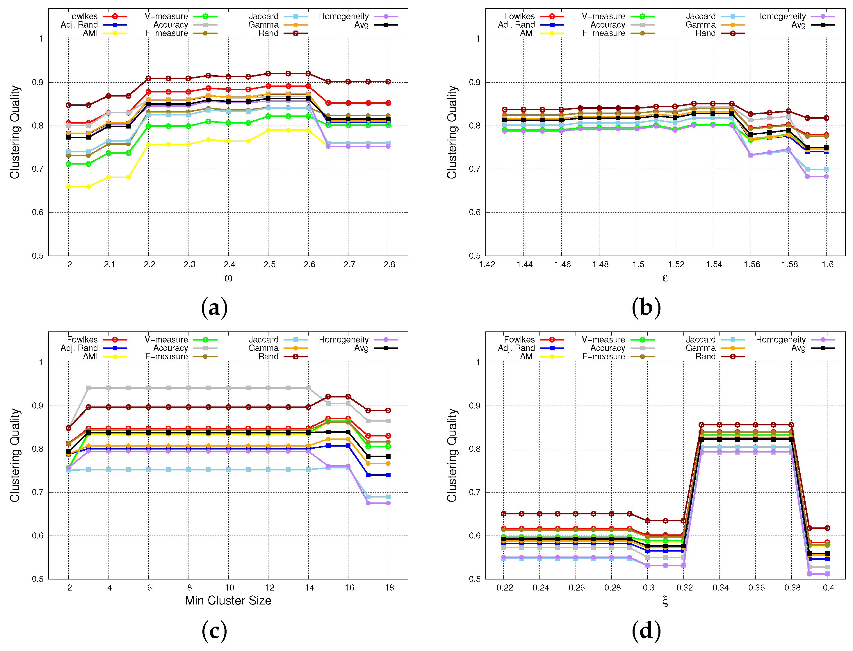
Similarly, we run several tests on the compound dataset, whose results are reported in Figure 5. In particular, the figure shows how quality indices vary versus input parameter values. We can observe that, even for this dataset, input parameter values strongly affect the clustering quality and performance index values. As a result, we find that CHD achieves the best result for ω * = 2.50 , DBSCAN for ϵ * = 1.53 , HDBSCAN for m i n _ c l u s t e r _ s i z e * = 15 and OPTICS-Xi for ξ * = 0.33 .
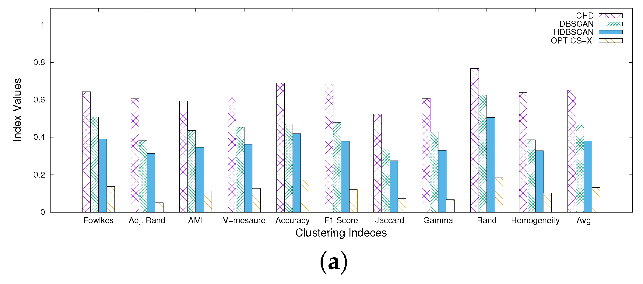
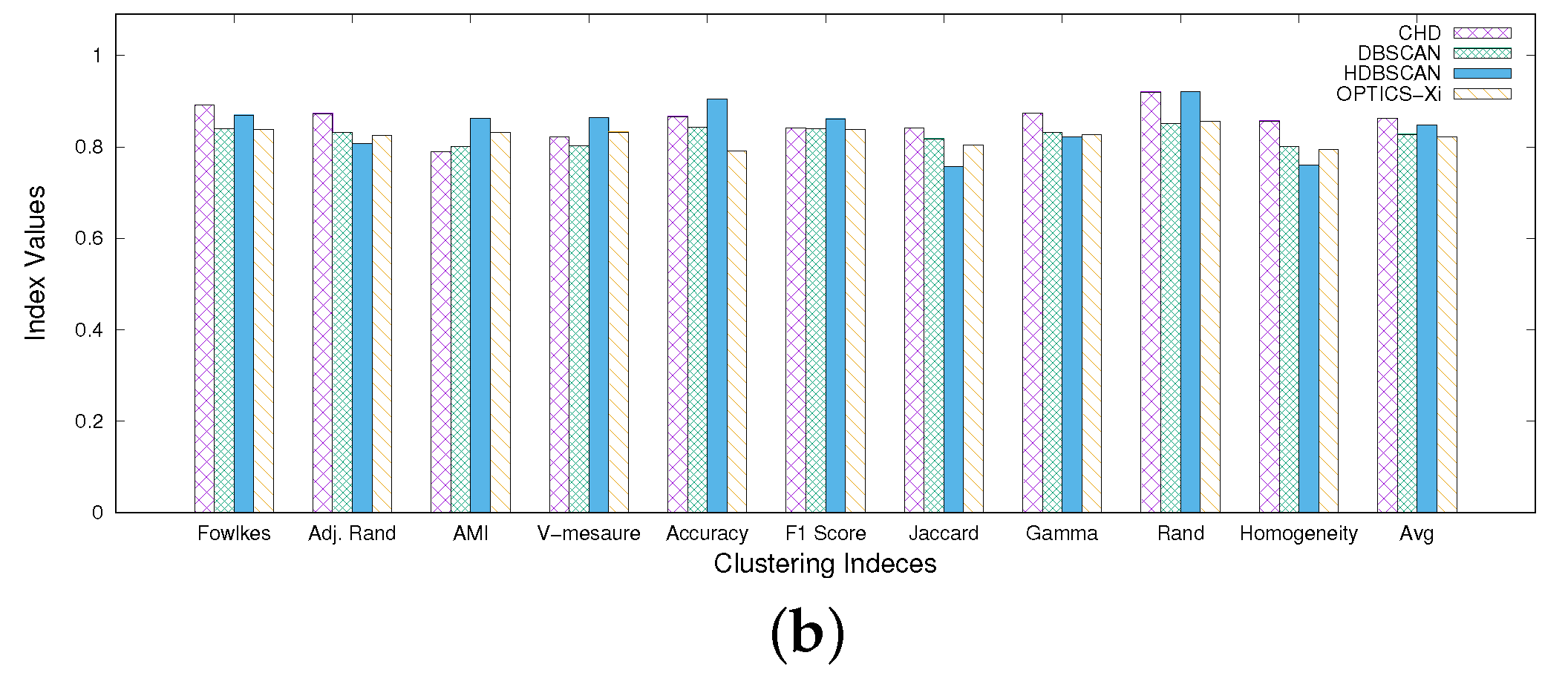
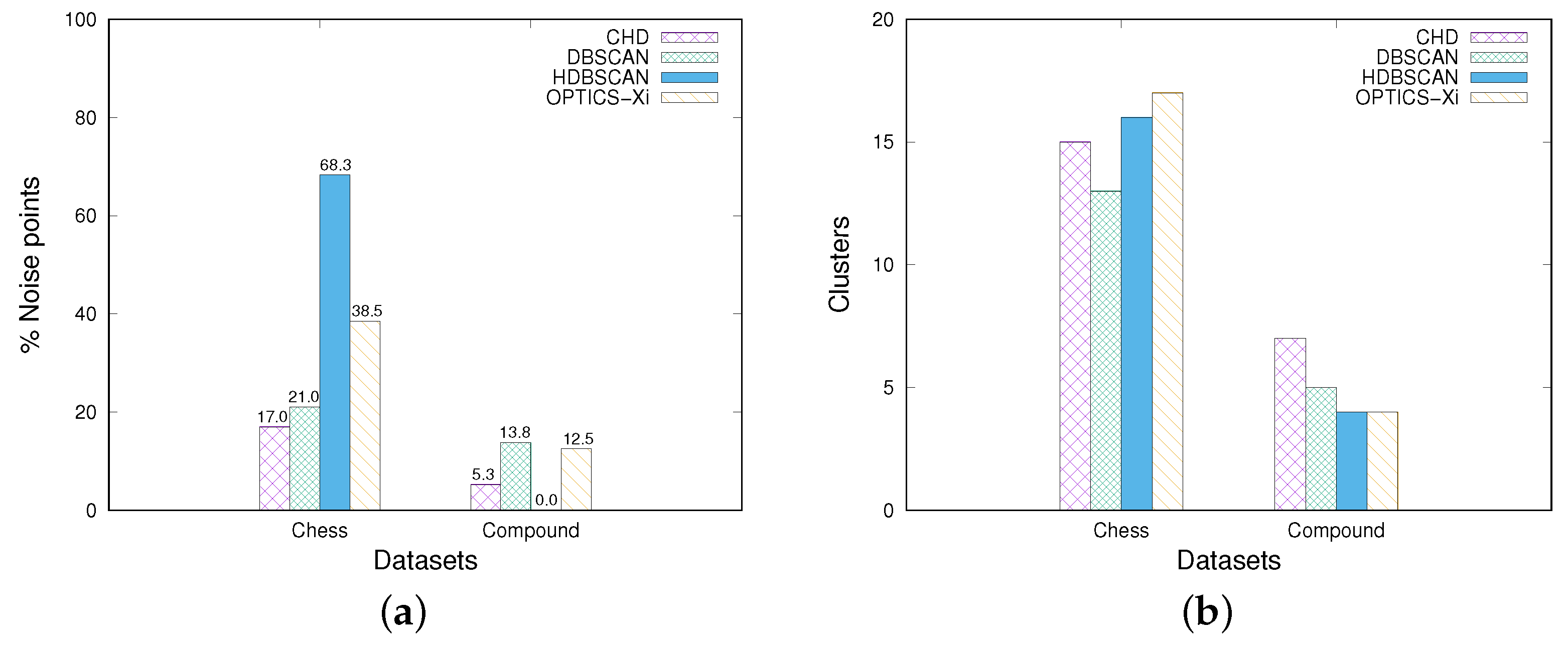
A quantitative performance comparison among the considered algorithms is presented in Figure 6, where the values of the clustering indexes are shown for chess and compound datasets, by only referring to the run with the best combination of input parameters. In addition, Figure 7 plots the number of noise points and the number of detected clusters for both datasets. From the presented results, we can make the following considerations:
-
CHD detects higher quality clusters than DBSCAN, HDBSCAN and OPTICS-Xi. For both datasets, in fact, Figure 6 shows that CHD achieves better performance than the other three algorithms, for all indices. Specifically, on chess, considering the best parameter setting case for each algorithm, CHD achieves an average clustering quality (computed over all indices) equal to 0.65, while DBSCAN, HDBSCAN, and OPTICS-Xi achieve 0.47, 0.38 and 0.13, respectively. Similarly, on compound, CHD slightly outperforms the other three algorithms, assessing on an average clustering quality equal to 0.86, while DBSCAN, HDBSCAN, and OPTICS-Xi achieve 0.83, 0.84, and 0.82, respectively. This is an interesting result since it shows that a multi-density approach, applied over such datasets, overtakes the other algorithms in terms of accuracy, compactness, and separability. In addition, the higher the closeness among clusters (chess dataset), the more evident the clustering quality improvement.
-
CHD and HDBSCAN detect a lower number of noise points than DBSCAN, and OPTICS-Xi. Figure 7 shows the number of noise points and the number of clusters detected by the two algorithms. Specifically, Figure 7a shows that CHD, on the Chess dataset, is the algorithm detecting the lowest number of noise points (17%). On the compound dataset, HDBSCAN detects no noise points, while CHD detects the 5.3% of the total number of instances, which is a very low number as well. The other two algorithms detect a higher number of noise points.
-
CHD largely outperforms the other algorithms when detecting not-well-separated clusters. Observing Figure 2 and Figure 3, we can observe that the chess dataset shows clusters that are very contiguous and not-well-separated, while in the compound dataset, the separation among clusters is more evident. Generally, the low separation between clusters is a crucial issue for density-based algorithms to detect proper clusters. Considering the results of our tests performed on both datasets, it is worth noting that, in particular on the chess dataset, CHD outperforms the other three algorithms, for all indices (see Figure 6). This means that its application results in being more effective than the other approaches when clusters are very close, which is a classic urban case scenario. On the compound dataset (see Figure 6), characterized by well-separated clusters, all four algorithms achieve good results, and the difference in their performance is less evident than in the first dataset.
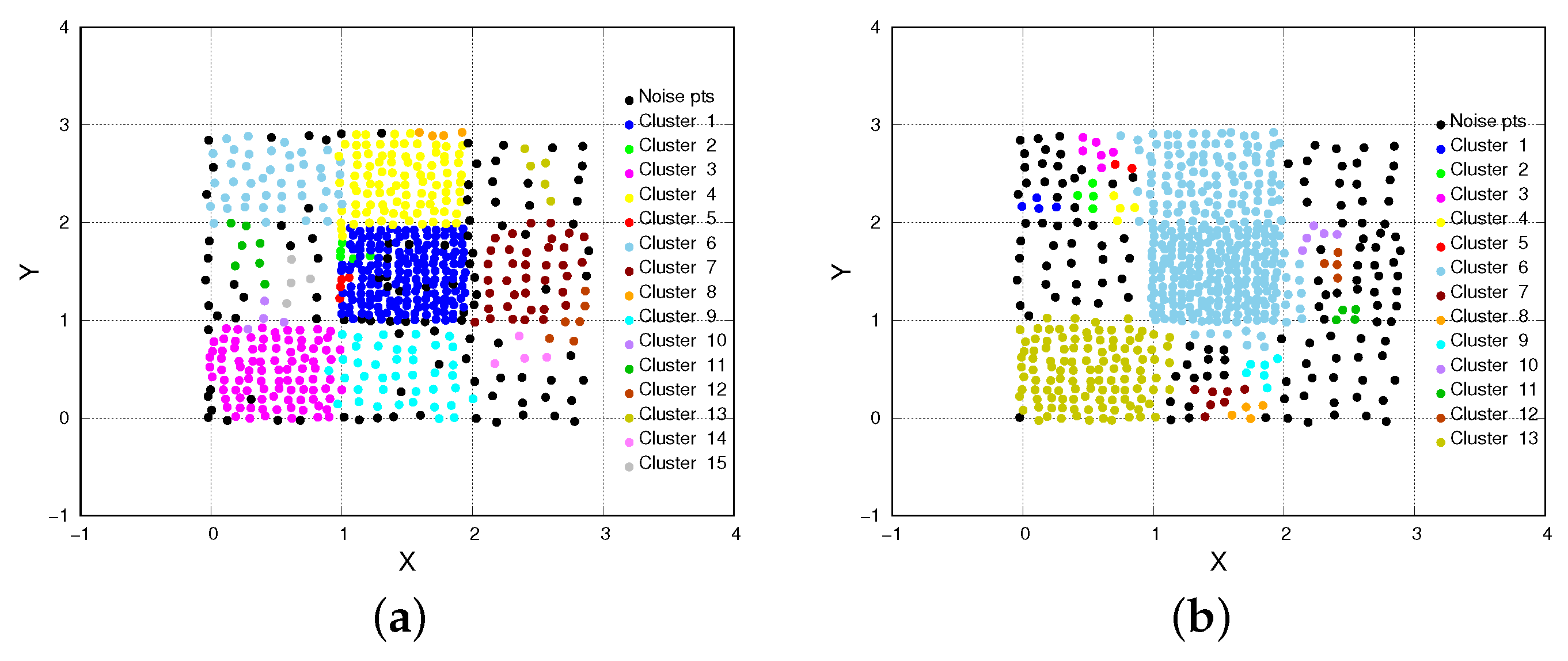
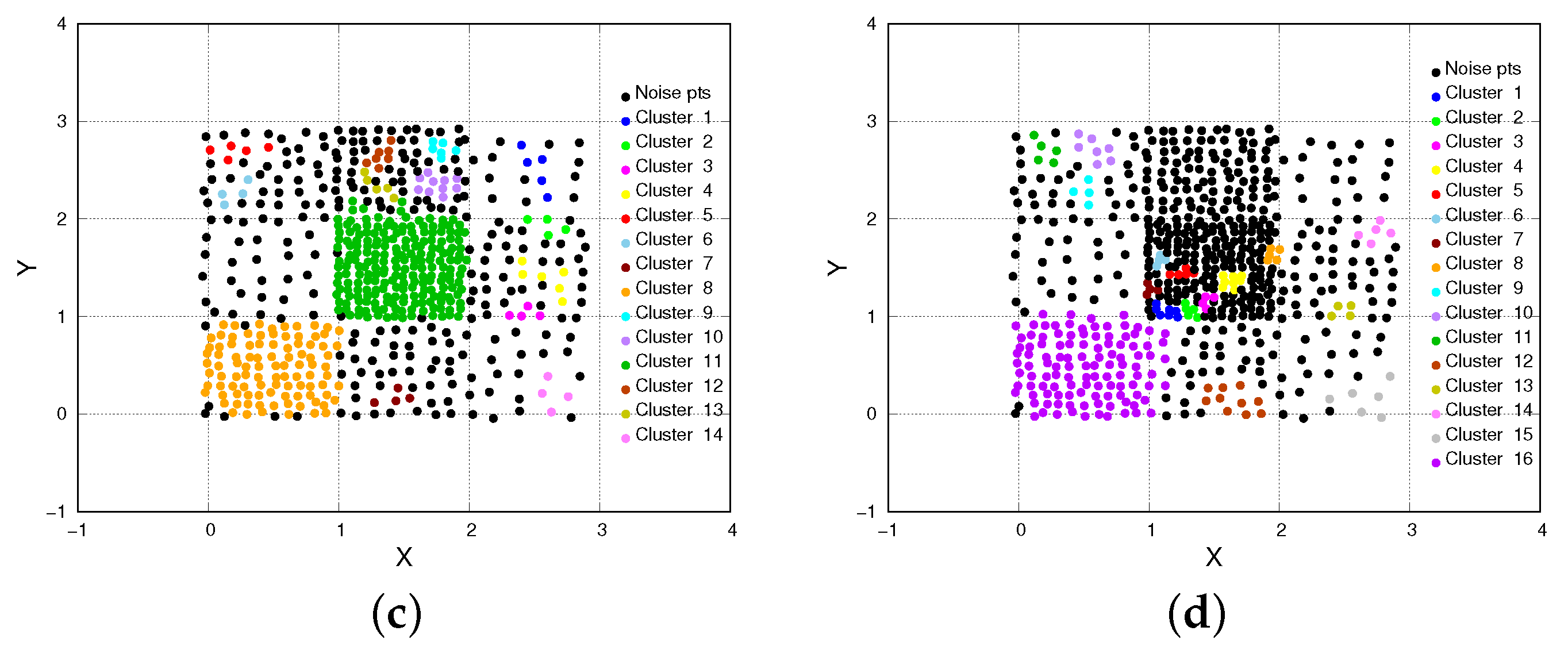
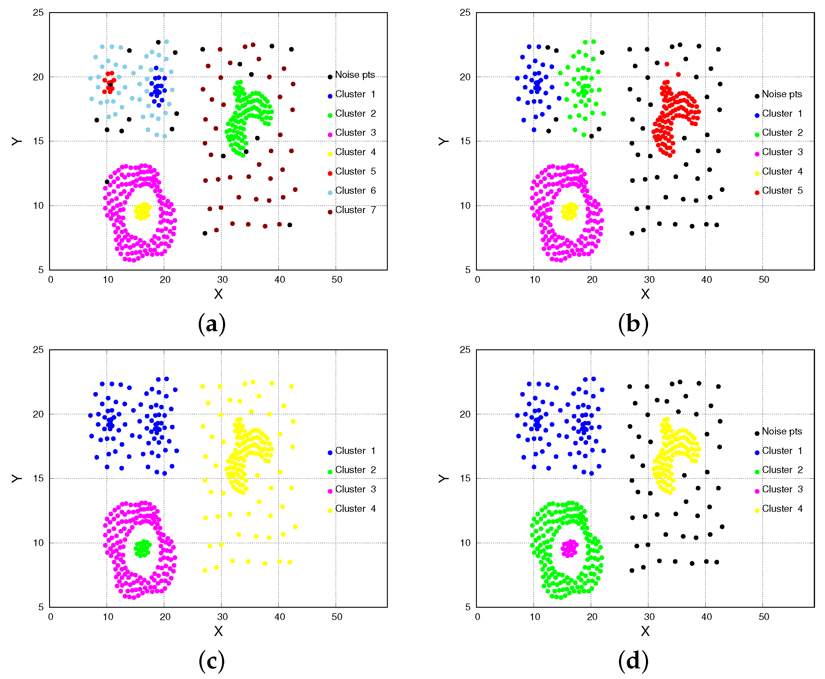
Finally, Figure 8 and Figure 9 show a qualitative comparison among the clustering models detected by the four algorithms on the two datasets. In particular, by observing Figure 8 (chess dataset) we can see that CHD detects 15 clusters, separability is quite good, and the number of noise points (in black) is very low with respect to the other algorithms. On the other side, DBSCAN and HDBSCAN detect a lower number of clusters than CHD, but a high number of noise points. Finally, OPTICS-Xi labels many instances as noise points, which makes the clustering quality very low. On the other side, by observing Figure 9 (compound dataset), we can see that the CHD and DBSCAN achieve a good separability among all clusters, while HDBSCAN and OPTICS-Xi are not able to separate the two clusters on the upper left side (cluster 1). It is worth noting that DBSCAN, OPTICS-Xi, and HDBSCAN could not detect the large low-density cluster on the right (cluster 1 in Figure 3b), labeling it as noise. That cluster is detected only by CHD.

5. A Real-Case Study: Detecting Multi-Density Crime Hotspots in Chicago

To evaluate the performance and assess the effectiveness of the approaches described in Section 3 to discover city hotspots in a real-world scenario, we perform a comparative evaluation on geo-referenced crime events collected over a large area of Chicago. In particular, such tests aim at showing a concrete use case on which density-based clustering analysis can be exploited and the practical usefulness of the selected clustering algorithms to discover city hotspots in real urban cases.

5.1. Data Description

The experimental evaluation presented in this section is performed on the ’Crimes—2001 to present’ dataset, consisting of a collection of crime events that occurred in Chicago from January 2001 to the present. The dataset is publicly available on the Chicago Data Portal (https://data.cityofchicago.org/, accessed on 18 December 2022), which also collects and provides open data about various aspects and events of Chicago, e.g., food inspection, traffic crashes, and COVID-19 vaccine diffusion. Each crime in the dataset is both geo-localized (with latitude and longitude) and time-stamped. Furthermore, it includes attributes describing other characteristics of each crime event, e.g., the FBI code and the crime type.
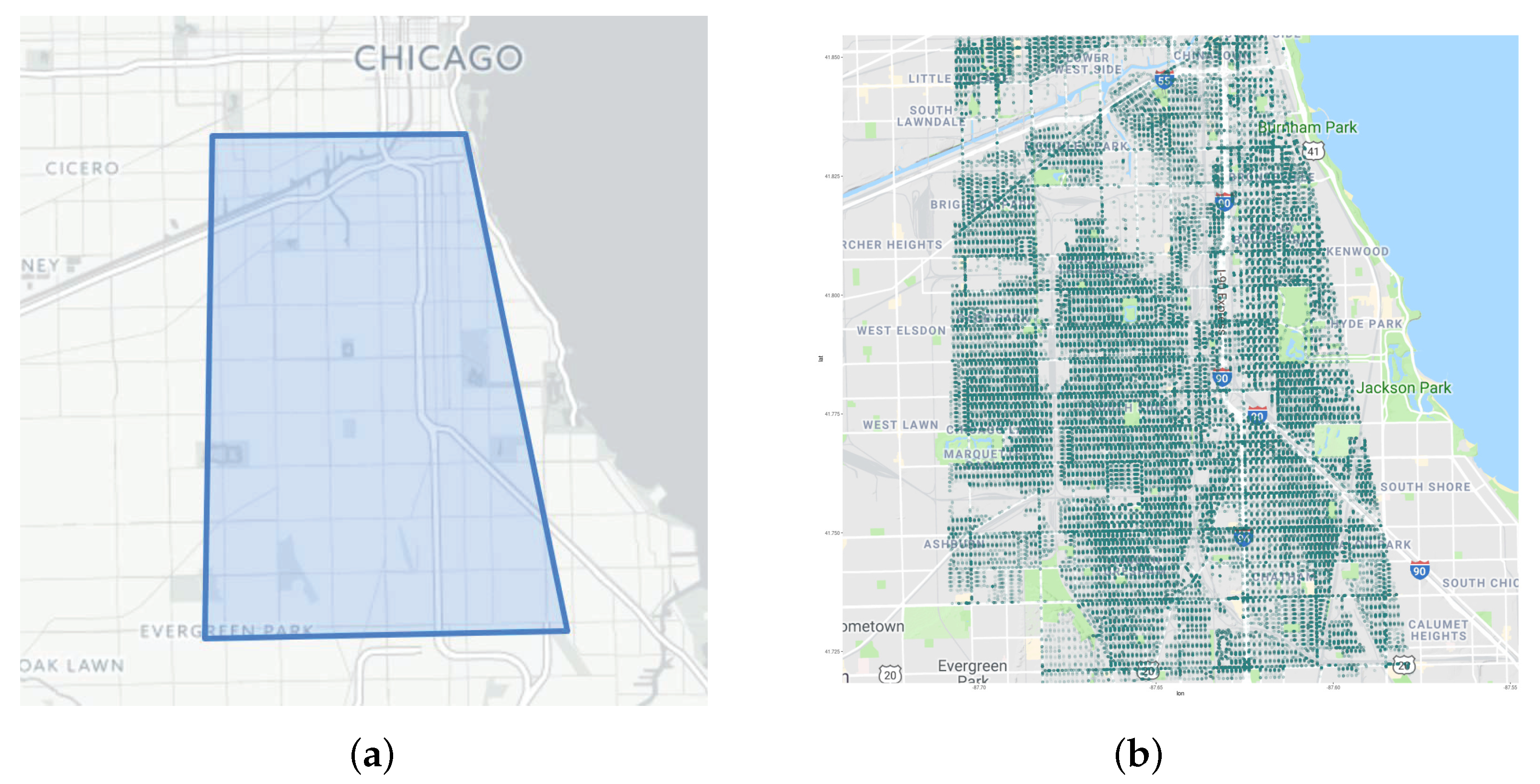
For the sake of our experimental evaluation, we consider only the latitude and longitude of crime events that occurred in 2012 and localized inside the boundary box shown in Figure 10a,b. The area has a perimeter of about 52 km and extends on approximately 135 km. The total number of crime instances is 100,219. The area includes different zones of the city, such as residential, commercial, tourist, and cultural zones, each one characterized by different crime densities. Given such a property, detecting urban hotspots in the area is a good benchmark to compare the performance results of the selected algorithms.

5.2. Results

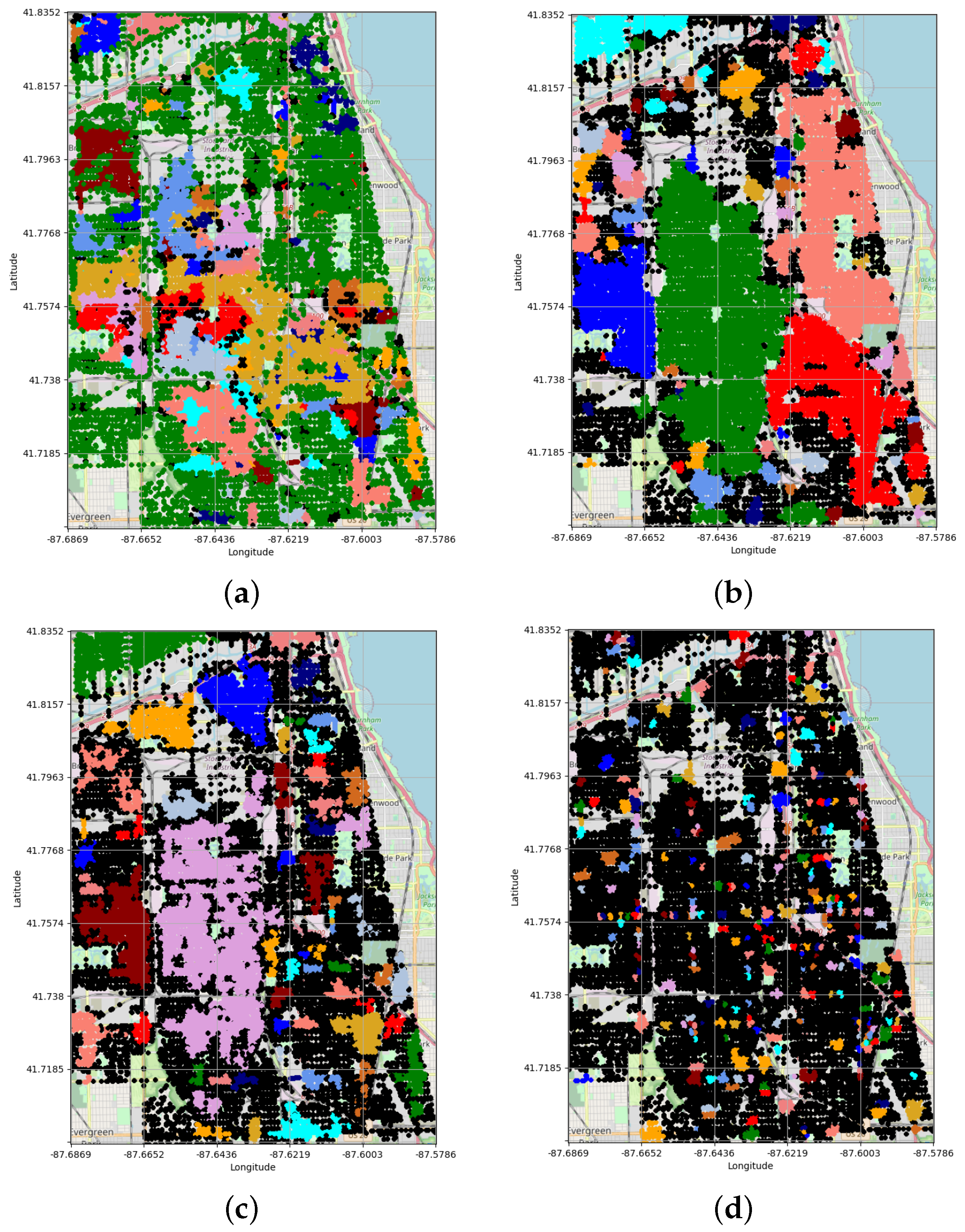
Similarly to the experimental evaluation performed on state-of-art datasets, we first assessed the best parameter settings for a fair comparison between CHD, DBSCAN, HDBSCAN, and OPTICS-Xi. We run several experimental tests to find the parameter settings capable of detecting the highest-quality city hotspots in terms of significance, compactness, and separability. Table 2 shows, for each algorithm, the selected input parameters and some statistics related to the achieved results. In particular, for each algorithm, the table reports the input parameter setting, the number of detected hotspots, the percentage of noise points, and the achieved Silhouette index values. In particular, Silhouette is an internal criterion to compute and evaluate clustering quality, and it is a measure of how similar an object is to its own cluster (cohesion) compared to other clusters (separation). The silhouette ranges from −1 to +1, where high values indicate that instances are well-matched to their own cluster and poorly matched to neighboring clusters. Thus, the higher the Silhouette value, the better the clustering quality (a more detailed description of this metric is reported in [33]). The hotspots detected by the considered algorithms are depicted in Figure 11, where they are highlighted through different colors, while noise points are black-colored.
Now, by observing the hotspots detected by the algorithms and shown in Figure 11, and the values reported in Table 2, we can make some considerations:
-
CHD detects a higher number of significant hotspots than DBSCAN, HDBSCAN and OPTICS-Xi. After a preliminary split in several density level sets, CHD partitions each one by exploiting specific ϵ values (as described in Section 3), finally detecting 181 hotspots; on the other side, DBSCAN and HDBSCAN detect a lower number of clusters, i.e., 78 and 61 hotspots, respectively. Finally, OPTICS-Xi detects 279 (very small) hotspots, which are not very significant.
-
CHD performs higher separation among the hotspots than DBSCAN, HDBSCAN and OPTICS-Xi. The results depicted in Figure 11 highlight that CHD is able to achieve a more refined spatial partitioning than DBSCAN and HDBSCAN, splitting some areas of the city. Contrariwise, OPTICS-Xi detected a large number of noise points and a lot of very small hotspots. In particular, CHD detects several hotspots in the central area (colored in red, orange, violet, and blue in Figure 11a, whereas DBSCAN and HDBSCAN labeled such points as only a single hotspot (the large green area in Figure 11b and the large violet area in Figure 11c). Similarly, CHD detects different hotspots in the left-middle part of the analyzed area, while DBSCAN and HDBSCAN label those as only one hotspot (colored in blue and red). OPTICS-Xi fails in a reasonable clustering of points, by detecting only some small hotspots sparsely distributed in the whole area. This shows that CHD is able to perform higher separation than the other algorithms among the city hotspots, by creating clusters having different densities.
-
CHD labels a lower number of noise points than DBSCAN, HDBSCAN, and OPTICS-Xi. The noise points, which are those points that could not be assigned to a hotspot since they do not satisfy the density requirements of a given algorithm, are colored in black in Figure 11. Table 2 reports that CHD, DBSCAN, and HDBSCAN classify 5.7%, 12.6%, and 34.6% of data instances as noise points, respectively. On the other side, OPTICS-Xi labels almost 72% of total points as noise, showing de facto low-quality results. Considering the first three algorithms, it seems that CHD, in several cases, is able to better detect hotspots characterized by distinct densities, labeling a low percentage of instances as noise points. This is clearly evident by comparing Figure 11a–c. In particular, we can notice that large regions located in the top part and bottom part of the analyzed area are labeled as noise by DBSCAN and HDBSCAN (black-colored blows in Figure 11b,c), while CHD is able to detect several clusters from it (several hotspots colored in green and blue in Figure 11a). Finally, the presence of noise points in Figure 11d is pervasive and diffused, showing low-quality results achieved by OPTICS-Xi.
-
HDBSCAN and CHD achieve higher clustering quality than DBSCAN and OPTICS-Xi. Table 2 shows that HDBSCAN and CHD assess on silhouette values equal to 0.19 and 0.23 , respectively. Indeed, they achieve better results than DBSCAN and OPTICS-xi, whose clustering quality assess on 0.28 and 0.46 . Such results show that multi-density clustering (i.e., HDBASCN and CHD) is able to distinguish several density regions and identify proper hotspots in urban environments better than DBSCAN and OPTICS-xi.

6. Conclusions

Detecting urban hotspots in smart cities is a challenging task, due to the fact that geo-spatial urban data, e.g., traffic, crimes, mobility, and events, are generally characterized by multiple densities that can differ widely from one area to another. This paper discussed research issues, challenges and approaches to discover multi-density hotspots in urban areas. Then, it compared the performance of four approaches (i.e., DBSCAN, OPTICS-xi, HDBSCAN, and CHD) available in the literature, and analyzed their performance on synthetic and real-world data. The evaluation on synthetic datasets was performed considering the best parameter setting for each algorithm, selected by a parameter sweeping methodology taking into account several quantitative clustering indexes. Similarly, a qualitative comparison of the different algorithms was performed on real urban data. Overall, the results showed that multi-density clustering algorithms (CHD and HDBSCAN) outperform classic density-based algorithms (DBSCAN and OPTICS-xi) when analyzing data characterized by multiple densities. Therefore, multi-density approaches are more appropriate for urban hotspot detection.

Author Contributions

Conceptualization, E.C. and A.V.; methodology, E.C. and A.V.; software, P.L. and A.V.; validation, E.C. and P.L.; formal analysis, E.C., P.L. and A.V.; investigation, P.L. and A.V.; resources, E.C. and P.L.; data curation, E.C., P.L. and A.V.; writing—original draft preparation, E.C. and A.V.; writing—review and editing, E.C., P.L. and A.V.; visualization, E.C., P.L. and A.V.; supervision, E.C. and A.V.; funding acquisition, E.C. and A.V.; All authors have read and agreed to the published version of the manuscript.

Funding

This work has been partially supported by the “ICSC National Centre for HPC, Big Data and Quantum Computing” (CN00000013) within the NextGenerationEU program, and by European Union—NextGenerationEU—National Recovery and Resilience Plan (Piano Nazionale di Ripresa e Resilienza, PNRR)—Project: “SoBigData.it—Strengthening the Italian RI for Social Mining and Big Data Analytics”—Prot. IR0000013—Avviso n. 3264 del 28/12/2021.

Data Availability Statement

The analyzed datasets are available as follows. The chess dataset is available at https://gitlab.com/chd3/datasets, accessed on 28 December 2022. The compound dataset is available at http://cs.joensuu.fi/sipu/datasets/, accessed on 18 December 2022. The Chicago “Crimes—2001 to present” dataset is available at https://data.cityofchicago.org/Public-Safety/Crimes-2001-to-Present/ijzp-q8t2, accessed on 18 December 2022.

Conflicts of Interest

The authors declare no conflict of interest.

References

  1. Li, L.; Jiang, R.; He, Z.; Chen, X.; Zhou, X. Trajectory data-based traffic flow studies: A revisit. Transp. Res. Part C Emerg. Technol. 2021, 114, 225–240. [Google Scholar]
  2. Cesario, E.; Comito, C.; Talia, D. An approach for the discovery and validation of urban mobility patterns. Pervasive Mob. Comput. 2017, 42, 77–92. [Google Scholar]
  3. Ali, M.E.; Hasan, M.F.; Siddiqa, S.; Molla, M.M.; Nasrin Akhter, M. FVM-RANS Modeling of Air Pollutants Dispersion and Traffic Emission in Dhaka City on a Suburb Scale. Sustainability 2022, 15, 673. [Google Scholar] [CrossRef]
  4. Wang, Q.; Jin, G.; Zhao, X.; Feng, Y.; Huang, J. CSAN: A neural network benchmark model for crime forecasting in spatio-temporal scale. Knowl.-Based Syst. 2020, 189, 105–120. [Google Scholar] [CrossRef]
  5. Catlett, C.; Cesario, E.; Talia, D.; Vinci, A. Spatio-temporal crime predictions in smart cities: A data-driven approach and experiments. Pervasive Mob. Comput. 2019, 53, 62–74. [Google Scholar]
  6. Chintalapudi, N.; Battineni, G.; Amenta, F. COVID-19 virus outbreak forecasting of registered and recovered cases after sixty day lockdown in Italy: A data driven model approach. J. Microbiol. Immunol. Infect. 2020, 53, 396–403. [Google Scholar] [PubMed]
  7. Ghosh, S.; Bhattacharya, S. A data-driven understanding of COVID-19 dynamics using sequential genetic algorithm based probabilistic cellular automata. Appl. Soft Comput. 2020, 96, 106692. [Google Scholar] [CrossRef] [PubMed]
  8. Hu, S.; Xiong, C.; Yang, M.; Younes, H.; Luo, W.; Zhang, L. A big-data driven approach to analyzing and modeling human mobility trend under non-pharmaceutical interventions during COVID-19 pandemic. Transp. Res. Part C Emerg. Technol. 2021, 124, 102955. [Google Scholar] [CrossRef] [PubMed]
  9. Cicirelli, F.; Guerrieri, A.; Mastroianni, C.; Spezzano, G.; Vinci, A. The Internet of Things for Smart Urban Ecosystems; Springer: Cham, Switzerland, 2019. [Google Scholar]
  10. Liu, P.; Zhou, D.; Wu, N. VDBSCAN: Varied density based spatial clustering of applications with noise. In Proceedings of the 2007 International Conference on Service Systems and Service Management, Chengdu, China, 9–11 June 2007; pp. 1–4. [Google Scholar]
  11. Mitra, S.; Nandy, J. KDDclus: A simple method for multi-density clustering. In Proceedings of the International Workshop on Soft Computing Applications and Knowledge Discovery (SCAKD 2011), Moscow, Russia, 24 June 2011; pp. 72–76. [Google Scholar]
  12. Cesario, E. Big Data Analysis for Smart City Applications. In Encyclopedia of Big Data Technologies; Sakr, S., Zomaya, A.Y., Eds.; Springer: Cham, Switzerland, 2019. [Google Scholar] [CrossRef]
  13. Canino, M.P.; Cesario, E.; Vinci, A.; Zarin, S. Epidemic forecasting based on mobility patterns: An approach and experimental evaluation on COVID-19 Data. Soc. Networks Anal. Min. 2022, 12, 116. [Google Scholar]
  14. Mastroianni, C.; Cesario, E.; Giordano, A. Efficient and scalable execution of smart city parallel applications. Concurr. Comput. Pract. Exp. 2018, 30, e4258. [Google Scholar] [CrossRef]
  15. Garrett Dash Nelson. What Micro-Mapping a City’s Density Reveals. 9 May 2021. Available online: https://www.bloomberg.com/news/articles/2019-07-09/what-micro-mapping-a-city-s-density-reveals (accessed on 18 December 2022).
  16. Organisation for Economic Cooperation and Development (OECD). Rethinking Urban Sprawl; OECD: Paris, France, 2018; p. 168. [Google Scholar] [CrossRef]
  17. Center for International Earth Science Information Network—CIESIN—Columbia University. Gridded Population of the World, Version 4 (GPWv4): Population Count, Revision 11, NASA Socioeconomic Data and Applications Center (SEDAC). 2021. Available online: https://sedac.ciesin.columbia.edu/data/set/gpw-v4-population-count-rev11 (accessed on 18 December 2022). [CrossRef]
  18. Deng, T.; Manders, A.; Jin, J.; Lin, H.X. Clustering-based spatial transfer learning for short-term ozone forecasting. J. Hazard. Mater. Adv. 2022, 8, 100168. [Google Scholar]
  19. Krupnova, T.G.; Rakova, O.V.; Bondarenko, K.A.; Tretyakova, V.D. Environmental Justice and the Use of Artificial Intelligence in Urban Air Pollution Monitoring. Big Data Cogn. Comput. 2022, 6, 75. [Google Scholar] [CrossRef]
  20. Khan, A.N.; Iqbal, N.; Rizwan, A.; Ahmad, R.; Kim, D.H. An Ensemble Energy Consumption Forecasting Model Based on Spatial-Temporal Clustering Analysis in Residential Buildings. Energies 2021, 14, 3020. [Google Scholar] [CrossRef]
  21. Kolevatova, A.; Riegler, M.A.; Cherubini, F.; Hu, X.; Hammer, H.L. Unraveling the Impact of Land Cover Changes on Climate Using Machine Learning and Explainable Artificial Intelligence. Big Data Cogn. Comput. 2021, 5, 55. [Google Scholar] [CrossRef]
  22. Cesario, E.; Marozzo, F.; Talia, D.; Trunfio, P. SMA4TD: A social media analysis methodology for trajectory discovery in large-scale events. Online Soc. Netw. Media 2017, 3–4, 49–62. [Google Scholar]
  23. Tayebi, M.; Ester, M.; Glasser, U.; Brantingham, P. CRIMETRACER: Activity space based crime location prediction. In Proceedings of the Advances in Social Networks Analysis and Mining (ASONAM), 2014 IEEE/ACM International Conference, Beijing, China, 17–20 August 2014; pp. 472–480. [Google Scholar]
  24. Kianmehr, K.; Alhajj, R. Crime Hot-Spots Prediction Using Support Vector Machine. In Proceedings of the Computer Systems and Applications, IEEE International Conference, Dubai, United Arab Emirates, 8 March 2006; pp. 952–959. [Google Scholar]
  25. Zhuang, Y.; Almeida, M.; Morabito, M.; Ding, W. Crime Hot Spot Forecasting: A Recurrent Model with Spatial and Temporal Information. In Proceedings of the 2017 IEEE International Conference on Big Knowledge (ICBK), Hefei, China, 9–10 August 2017. [Google Scholar]
  26. Ester, M.; Kriegel, H.P.; Sander, J.; Xu, X. A density-based algorithm for discovering clusters in large spatial databases with noise. In Proceedings of the Second International Conference on Knowledge Discovery and Data Mining, Portland, OR, USA, 2–4 August 1996; Volume 96, pp. 226–231. [Google Scholar]
  27. Ankerst, M.; Breunig, M.M.; Kriegel, H.P.; Sander, J. OPTICS: Ordering points to identify the clustering structure. In Proceedings of the ACM Sigmod Record, Philadelphia, PA, USA, 1–3 June 1999; Volume 28, pp. 49–60. [Google Scholar]
  28. Campello, R.J.; Moulavi, D.; Zimek, A.; Sander, J. Hierarchical density estimates for data clustering, visualization, and outlier detection. ACM Trans. Knowl. Discov. Data (TKDD) 2015, 10, 1–51. [Google Scholar] [CrossRef]
  29. Müller, D.W.; Sawitzki, G. Excess mass estimates and tests for multimodality. J. Am. Stat. Assoc. 1991, 86, 738–746. [Google Scholar]
  30. Cesario, E.; Uchubilo, P.I.; Vinci, A.; Zhu, X. Multi-density urban hotspots detection in smart cities: A data-driven approach and experiments. Pervasive Mob. Comput. 2022, 86, 101687. [Google Scholar] [CrossRef]
  31. Fränti, P.; Sieranoja, S. K-Means Properties on Six Clustering Benchmark Datasets. 2018. Available online: http://cs.uef.fi/sipu/datasets/ (accessed on 18 December 2022).
  32. Zahn, C. Graph-theoretical methods for detecting and describing gestalt clusters. IEEE Trans. Comput. 1971, 100, 68–86. [Google Scholar]
  33. Jain, A.; Dubes, R. Algorithms for Clustering Data; Prentice-Hall: Hoboken, NJ, USA, 1988. [Google Scholar]
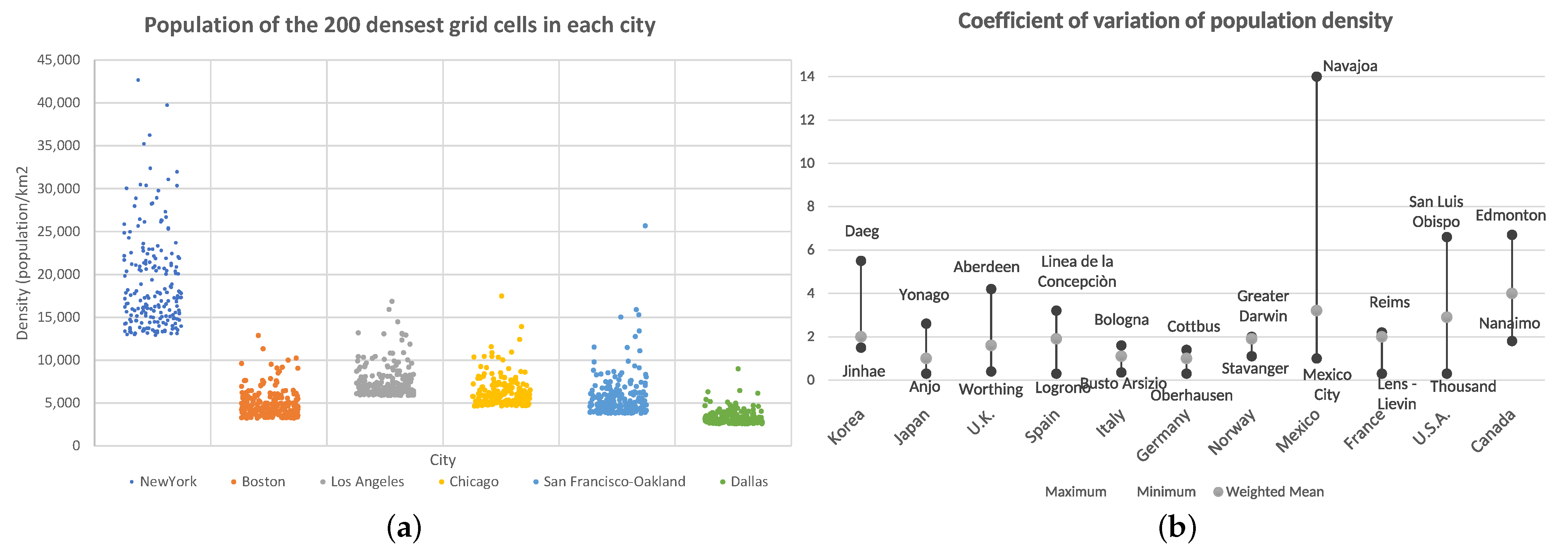
Figure 1. Intra-city and inter-city population densities in metropolitan urban areas. (a) Population densities of the densest 200 cells for a given set of cities. Each cell has a 1 km2 area [17]. (b) Coefficient of variation of population density across urban areas and countries (2014) [16]. For each country, the gray dot is the average computed on the coefficient of variation of each city of the country. The figure also displays, for each country, the minimum and the maximum coefficients of variation, and the cities where they occur.
Bdcc 07 00029 g001
Figure 2. The Chess dataset: (a) data instances and (b) target clusters.
Bdcc 07 00029 g002
Figure 3. The Compound dataset: (a) data instances and (b) target clusters.
Bdcc 07 00029 g003
Figure 4. The Chess dataset: clustering quality indices vs. different input parameter values. (a) CHD. (b) DBSCAN. (c) HDBSCAN. (d) OPTICS-Xi.
Bdcc 07 00029 g004
Figure 5. The Compound dataset: clustering quality indices vs. different input parameter values. (a) CHD. (b) DBSCAN. (c) HDBSCAN. (d) OPTICS-Xi.
Bdcc 07 00029 g005
Figure 6. Best clustering results for the four algorithms on the two datasets: chess (a) and compound (b) datasets.
Bdcc 07 00029 g006aBdcc 07 00029 g006b
Figure 7. Number of noise points (a) and number of clusters (b) detected by the four algorithms on the two datasets.
Bdcc 07 00029 g007
Figure 8. The Chess dataset: detected clusters. (a) CHD. (b) DBSCAN. (c) HDBSCAN. (d) OPTICS-Xi.
Bdcc 07 00029 g008aBdcc 07 00029 g008b
Figure 9. The Compound dataset: detected clusters. (a) CHD. (b) DBSCAN. (c) HDBSCAN. (d) OPTICS-Xi.
Bdcc 07 00029 g009
Figure 10. Selected area of Chicago and geo-localized crime events. (a) Polygon of the area; (b) geo-localized crime events.
Bdcc 07 00029 g010
Figure 11. The Crime dataset: detected clusters. (a) CHD. (b) DBSCAN. (c) HDBSCAN. (d) OPTICS-Xi.
Bdcc 07 00029 g011
Table 1. Experimental setting for the parameter sweeping for each algorithm.
DatasetAlgorithmFixed ParameterSwept ParameterBeginEndBest Average PerformanceBest Swept Parameter Value
ChessCHD k = 4 , s = 1 ω 0.11.70.65 ω * = 1
DBSCAN m i n _ p t s = 4 ϵ 0.080.250.47 ϵ * = 0.14
HDBSCAN m i n _ p t s = 4 m i n _ c l u s t e r _ s i z e 2180.38 m i n _ c l u s t e r _ s i z e * = 3
OPTICS-Xi m i n _ p t s = 4 ξ 0.060.080.13 ξ * = 0.066
CompoundCHD k = 4 , s = 1 ω 2.02.80.86 ω * = 2.5
DBSCAN m i n _ p t s = 4 ϵ 1.431.60.83 ϵ * = 1.53
HDBSCAN m i n _ p t s = 4 m i n _ c l u s t e r _ s i z e 2180.84 m i n _ c l u s t e r _ s i z e * = 15
OPTICS-Xi m i n _ p t s = 4 ξ 0.20.40.82 ξ * = 0.33
Table 2. Overview of the results obtained by CHD, DBSCAN, HDBSCAN, and OPTICS-Xi.
Input Parameters# Hotspots# Noise PointsSilhouette Index
CHD ω = 0.27 , k = 64 , s = 5000 1815.7%−0.23
DBSCAN ϵ = 500 , m i n P o i n t s = 60 7812.6%−0.28
HDBSCAN m i n _ c l u s t e r _ s i z e = 200 , m i n P o i n t s = 60 6134.6%−0.19
OPTICS-Xi ξ = 0.05, m i n P o i n t s = 60 27971.9%−0.46
Disclaimer/Publisher’s Note: The statements, opinions and data contained in all publications are solely those of the individual author(s) and contributor(s) and not of MDPI and/or the editor(s). MDPI and/or the editor(s) disclaim responsibility for any injury to people or property resulting from any ideas, methods, instructions or products referred to in the content.