Explaining Intrusion Detection-Based Convolutional Neural Networks Using Shapley Additive Explanations (SHAP)

Abstract

Artificial intelligence (AI) and machine learning (ML) models have become essential tools used in many critical systems to make significant decisions; the decisions taken by these models need to be trusted and explained on many occasions. On the other hand, the performance of different ML and AI models varies with the same used dataset. Sometimes, developers have tried to use multiple models before deciding which model should be used without understanding the reasons behind this variance in performance. Explainable artificial intelligence (XAI) models have presented an explanation for the models’ performance based on highlighting the features that the model considered necessary while making the decision. This work presents an analytical approach to studying the density functions for intrusion detection dataset features. The study explains how and why these features are essential during the XAI process. We aim, in this study, to explain XAI behavior to add an extra layer of explainability. The density function analysis presented in this paper adds a deeper understanding of the importance of features in different AI models. Specifically, we present a method to explain the results of SHAP (Shapley additive explanations) for different machine learning models based on the feature data’s KDE (kernel density estimation) plots. We also survey the specifications of dataset features that can perform better for convolutional neural networks (CNN) based models.

1. Introduction

AI has become a basic building block in most advanced technological systems, aiming to provide decisions that are difficult to be performed by a human due to the nature of the data or the computations required. This reliance on AI systems makes decision justification a requirement to enable the trustworthiness of the ML models used. It is a fact that ML model accuracy depends highly on the input data, known as a dataset in the literature. The dataset’s quality is a major factor affecting the quality of the ML model’s performance and the goodness of its decisions.

Intrusion detection systems (IDS) are ML systems that have been extensively developed, in the recent literature, using several symmetric (such as neural networks inferencing systems) and asymmetric (such as fuzzy inferencing systems) computational intelligence techniques [1]. However, intrusion detection datasets used in training intrusion detection AI systems have been limited due to privacy issues [2]. In contrast, the commonly used datasets are vast and contain many records, each with many features listed. In [3], XAI models were used to build a two-stage intrusion detection model in a Wi-Fi network.

The explainable artificial intelligence, or the XAI concept, has come to attention due to its significant role in adding reliance and trust to decisions taken by artificial intelligence models. XAI can also shift decision liability towards artificial intelligence models and provide human operators with decision justification. Thus, human decisions built over artificial intelligence models are not taken blindly. XAI methods were proposed to explain decisions by artificial intelligence models based on the contribution of features to decisions. XAI methods can be classified into global and local methods according to whether we are trying to explain a single decision (symmetric) by the artificial intelligence model or all the decisions (asymmetric).

1.1. Explainable Artificial Intelligence

To date, AI has held a considerable role in intrusion detection models and many other aspects, such as the works presented in [4,5,6]. These results lack proper explanations and justifications regarding these results. Explainable AI or XAI systems such as SHAP and LIME (Local Interpretable Model-agnostic Explanations) can enable AI results to be more interpretable, trustful, and symmetrical to human decisions. XAI models work with a specific dataset within a specific ML model. XAI systems are tools built to justify AI results by highlighting the contribution of the dataset features to the AI results. These systems can explain the overall result or a single prediction, usually named global and local decisions [7].

The XAI methods used to interpret intrusion detection systems (IDS) were classified [8] into the white box and black box methods. The white box methods include regression, rule-based, clustering, and statistical and probabilistic methods. Black box approaches are composed of feature, perturbation, decomposition, and hybrid approaches. White box methods contain transparent code and can be used to investigate the details of the interpreting method. The extra transparency of the white box methods comes at the cost of accuracy [9] as well as usage simplicity [10]. According to [10], white box explanations should match black box explanations, while at the same time, black box explanations are more accurate and easier to generate.

Black box methods are XAI methods whose codes are not available for users. Perturbation-based approaches perform minor modifications to input data and obtain the change in predictions. These methods suffer from an out-of-ordered data problem which occurs when the AI model must deal with data that is inconsistent with the distribution of the original training dataset. Feature-based methods highlight features that have a major influence on the decision of an AI model. The most famous method belonging to this group of methods is SHAP.

In the literature, there are two famous methods that are widely used for XAI purposes. These methods are LIME and SHAP [11,12,13].

SHAP uses global and local explanations and can be used with variant ML and AI models such as artificial neural networks, decision trees, naïve bays, and many others. SHAP library can be imported into a Python code, and then the provided methods in the library can be used to explain the results of different AI and ML models.

LIME is an open-source framework built and designed to interpret decisions by ML models. Local and global decisions can be explained using LIME. LIME has three main scopes in which it can perform perfectly: the image explainer, which takes care of image classification ML models; the text explainer, which takes care of text-based models; and the tabular explainer, which provides an insight into the importance of tabular dataset features in a decision [14]. SHAP is another XAI framework built using game theory to create a framework that can explain AI prediction and visualize the origins of decisions. SHAP is explained and detailed in [15], while LIME can be referred to through [16].

Frameworks such as LIME and SHAP allowed ML models to derive justifications for the gained results; hence, the black box character of ML models became colored. The intelligence of the ML models became more robust and more reliable with the aid of XAI. XAI highlights the most important features of the dataset to be considered during decision-making. Such highlighted features can vary from one model to another model within the same dataset. In this study, we try to explain why and how this variance happens.

It is good to mention that XAI was deployed in fields other than intrusion detection. For example, the work in [17] presented three ML models for travel time prediction and supported the study with XAI results. Additionally, to add transparency to ML models predicting the future states of running instances of a business process, authors in [18] used LIME and SHAP XAI methods. Another noticeable example is the engineering approach for deploying configurable cloud applications proposed in [19]. The contributors have used XAI to add more reliability to their proposed model. Eventually, at the time, LIME and SHAP have shown reliable and frequent use in literature according to [20,21]; SHAP has shown better performance than LIME in many cases.

1.2. The Main Contributions of the Study

Intelligent IDS systems typically do not use XAI methods, despite the need to justify the decision taken by these systems [22]. White box XAI methods have their limitations regarding the accuracy and the required additional programming work [9,10], while block box methods can interpret the decision taken by AI models without explaining the details of how and why the XAI model has taken the decision.

Tabular datasets are commonly used with IDS systems. These datasets are composed of different features carried as columns inside the dataset. Each feature has a certain range of values, continuous or discrete; narrow or extended. In this work, we are interested in the features’ values and how they are distributed over their domains, and the degree of correlation between the features and the label’s KDE plots. This information is then linked into XAI methods results such as the famous SHAP method. The conclusions built on the SHAP results are later used to expect how AI models will interact with different features and datasets based on the features’ KDE plots. A method for feature selection from tabular datasets to be used with CNN models is also proposed and justified.

At the time, XAI provided a fair degree of trust for AI; however, XAI was questioned and criticized in many works, such as [22,23,24,25]. We noticed that XIA methods such as SHAP provide varying results when trained with the same dataset using different AI systems. Such varying results are the spark that started this study. We are interested in justifying the widely used SHAP results and expanding this justification to be a new hybrid XAI system that lies between white box and black box XAI methods.

This study provides an analytic approach to investigate why certain features are more important to a learning model than others, especially for CNN models. This study can help select the properly supervised learning model for certain datasets based on the features characteristics embedded inside the KDE plot for each feature; it also aims to aid in selecting accurate features for a learning model based on its architecture. This, in turn, reduces the training dataset size with minor effects on the attained accuracy, calibration, and model selection times. This study is a step forward in explaining XAI methods results compared to prior studies. Rather than explaining the ML model result, we explain why and how an XAI system highlights certain features’ importance. We consider this work as an extra layer of explainability added to state-of-the-art XAI methods to explain their results in choosing important features for an ML model.

The main contributions can be summarized into:

• Studying the XAI results for multiple ML and AI models in intrusion detection applications using the “KDD 99” and “Distilled Kitsune-2018” datasets.
• Interpreting and digging into the XAI results to understand which dataset features are more useful to an ML model based on the feature’s KDE characteristics.
• Present a methodology that can be used before building an ML model, which helps select the proper ML model for a certain dataset based on its KDE plot.
• Present a methodology to select the most important features of an AI model before applying XAI analysis to the ML model’s results.

This research focuses on explaining XAI results for a dataset widely used in intrusion detection research rather than studying the dataset itself. The work presents a method to look deeper and realize the amount and the nature of the information carried in each feature of the dataset. This would help select the proper ML model and understand its behavior with the dataset.

The rest of this paper is structured as follows: The state-of-the-art review and investigation is provided in Section 2. The framework for the proposed XAI model to explain the Intrusion Detection (ID)-based CNN is provided in Section 3. Section 4 presents the results obtained for: dataset classification, the performance of ML classifiers using different datasets, explaining XAI results for the models. The last section, Section 5, concludes the paper. We aim to explain the XAI results for the SHAP XAI method on the “KDD 99” and Distilled Kitsune-2018 intrusion detection datasets with the help of kernel density estimation functions. The features included in the “KDD 99” and Distilled Kitsune-2018 intrusion detection datasets showed that the data distribution for each feature could be one of two categories, either centered around certain values, which we named “dense”, or distributed in a relaxed shape over their range of values named “relaxed” through this study.

2. Related Work

Explaining the artificial intelligence for autonomous intelligent intrusion detection systems (IDS) has recently become one of the main interests of cybersecurity researchers. A better understanding of the data distribution employed to build, train, and validate the IDS models will help improve their performance and provide more insights about data impacts and correlations. The KDE function can be viewed as a linear, smooth representation of a data histogram. It gives a visual enlightening of where data are concentrated elegantly. Recently, density functions provided a deep understanding of data distribution.

Consequently, KDE has been employed as a core explaining function to provide more understanding and insights into the data of several AI-based models. For instance, the work presented in [26] studied the density of data features in a certain context. They studied the density of opcodes in data packets; for example, they realized that a packet containing the opcode ‘MOV’ tends to be safe in a network security context while the packets with ‘ADC’ and ‘SUB’ opcodes tend to be harmful. In the same context, the authors of [27] have realized that the KDE figure can be useful for ML models as it carries much information about data distribution and probabilities. Hence, they built their one-class classification tree based on the features of KDE plots. They presented a greedy and recursive approach that uses kernel density estimation to split a data subset based on single or multiple intervals of interest to build the one-class classification model. Unlike the work presented here, we used KDE plots to justify the model’s results rather than building the model. Additionally, interpretability presented in [27] focused on interpreting the results of one-class classification and clustering models explaining why and how the selected features of a classification tree were considered important. While for this study, the interpretability was discussed in a more comprehensive frame.

In the same context, authors of [28] employed the KDE plots to explain the AI-based intrusion detection system by visualizing the “class” feature distribution. Hence, the decisions were made based on threat heterogeneity but not on the XAI method, as they used SHAP as an XAI method. Specifically, KDE plots were used as a visual tool to illustrate the characteristics of the features in the datasets accumulated for DoH (DNS over HTTPS) attacks. Similarly, AI-based intrusion detection systems in [29] were explained using a customized SHAP-based XAI model. Moreover, the work presented in [30] compared different XAI methods in intrusion detection systems focusing on XAI methods results. We added in this study a method to justify such generated results based on features’ KDE plot for each feature.

While state-of-the-art XAI methods such as “LIME” and “SHAP” focused on explaining the results provided by ML models by emphasizing the importance of the dataset features and for different ML models [31], however, XAI methods did not explain or analyze why some features contribute more to an ML model rather than others. Furthermore, the figures and the statistical results provided by the XAI methods can be confusing and might lack clearance.

A thorough analysis of XAI methods was conducted in [24] focusing on challenges facing XAI, such as the lack of experts who can understand and assess the results of XAI, the changes in XAI results when the data or the ML model are changed, and the interference of algorithms and context dependency. This work comes to reveal some facts behind the decisions taken by XAI. The work in [32] emphasized that the black box XAI methods should have a reasonable degree of transparency to make them more reliable and acceptable. Moreover, features KDE plots were used in [33] to reflect the distribution of the dataset features’ values over their range of values. The importance of the KDE plots was to reflect whether the values of the features are normally distrusted or not. This was presented by showing the min–max normalization of the features to enhance the performance of their developed network traffic classification model. Features with multiple peaks existing in the KDE plots were believed to need normalization prior to the training process to enhance the model’s accuracy.

In [34], multiple ML models (such as Random Forest Classifier, Logistic Regression, KNN, Xgboost, Naïve Bayes, and Decision Tree) were used to classify and predict chronic kidney disease. They used the features’ KDE plots to visualize and study the correlation between different features. Correlated features seemed to be more beneficial in enhancing the models’ classification process.

The SHAP values were not used as an abstract XAI tool all the time. The provided results gained from SHAP can be used to provide a deep insight into the developed model or the used dataset. The work presented in [35] for an AI-based bearing fault diagnosis under different speed and load values has used the SHAP results in the feature selection process. The used feature selection method has helped to avoid the multicollinearity problem, which is familiar with these systems.

Finally, the works proposed in [33,34] used the features KDE plots to visualize how the features’ values are distributed over their ranges and enhance the dataset pre-processing and the feature selection processes.

In this work, we have realized that the carried information in the KDE plots might help explain the ML and the AI models’ performance according to KDE plots. We also believe that explaining the models’ results (i.e., XAI models’ results) can be helpful in selecting the best features for each model.

In Table 1 below, we list a summary of the works that used KDE plots to explore the data characteristics and the embedded information in the KDE plots. Other studies using XAI expand the generated interpretations into a useful form of action.

Table 1. Related works summary.

Study	XAI Tool	DataSet	Main Findings of the Study
[27]	None	Six different medical datasets	They presented an approach that uses kernel density estimation to split a data subset based on one or several intervals of interest to build the one-class classification model.
[30]	LIME, SHAP, Anchors, and LORE	SimpleWeb dataset and ISCX IDS 2012	They explored the feasibility of applying different XAI techniques in the intrusion detection domain. They used the results from the XAI systems to create a white-box ML model.
[36]	LIME, SHAP, and Others	NSL-KDD	They used a deep neural network for network intrusion detection and also proposed an XAI framework to make the stages of the ML pipeline more interpretable.
[26]	-	The dataset is created by representing opcode density histograms.	They proved that a subset of opcodes could be used to detect malware, and applying a filter to the features can reduce the SVM training phase.
[31]	SHAP, DeepLIFT, LRP, and Saliency Maps	FordA, FordB, ElectricDevices, and seven other relevant datasets	They showed that XAI methods with images and text work on time series data by specifying relevance to time points.
[4]	Decision Tree importance algorithm	KDD	They used the XAI concept to improve the decision tree model in the area of IDS. They improved simple decision tree algorithms that mimic a human decision-making approach.
[3]	SHAP	AWID-CLS-R	A two-stage classification model was proposed to detect intrusions in a Wi-Fi network. The first stage uses all the dataset features to make predictions, while the second stage uses the most important features in stage one.

3. Proposed XAI Mechanism

The research methodology followed through this work aims to visualize each feature’s data distribution and classify them according to their data distribution into dense and non-dense sub-datasets. Then, the behavior of model accuracy is studied and explained according to these features’ data distribution. Later, the features we believe are more important to CNNs were compared to SHAP analysis results. The proposed system methodology followed throughout this work is illustrated in Figure 1.

Figure 1. Methodology followed through this work.

SHAP calculates shapely values via a backpropagation method to measure the impact of every layer in the ML model on the layer coming after. The process starts from the result layer and propagates back through the layers reaching into the input layer. This backpropagation process helps highlight the most impacting input data in making the decision by the ML model being explained. SHAP provides visual results showing the features which have a positive or negative impact on a taken decision. Mathematically, SHAP produces an explanation in the form of a vector of importance scores or SHAP values. SHAP was described as the extension of LIME; at the time, LIME focused on local explanation only, while SHAP took care of both local and global explanation [37].

The datasets used in this study are the “KDD 99” and “Distilled Kitsune-2018” recently used with ML models in works such as [1,38,39]. The KDD 99 dataset was collected and prepared in MIT Lincoln Labs as a part of “The 1998 DARPA Intrusion Detection Evaluation Program”, aiming to evaluate research intrusion detection. The data were collected from a simulation environment similar to an actual Air Force environment. The attacks simulated a wide variety of intrusions, including denial-of-service (DOS), unauthorized access from a remote machine (R2L), and unauthorized access to local superuser (root) privileges (U2R) and probing.

We specifically used a subset of the data labeled as “anomaly” for malicious connections and “normal” for benign non-intrusion connections regardless of the attack types for the anomaly attack type. The dataset features are 41, including the “class” feature, which states whether the connection is normal or an anomaly. The rest of the features are categorized into three basic sets of features. The three features describe the basic features of individual TCP connections, features based on domain knowledge, and traffic features, all computed using a two-second time slot. The dataset was interpreted and explained in [40].

In this work, a deep analysis of the dataset features was performed to interpret features contribution in different ML models. It also surveys specifications of dataset features that can result in better CNN model accuracy and performance. The methodology followed throughout this work is shown in Figure 1. The KDE function was calculated and plotted for each feature in the data set to visualize feature parameters and distribution. This analysis was conducted to visualize feature values distribution over their range of values. Before this step, every feature was normalized and remapped to range from 0 to 1.

KDE is a continuous representation of the features and represents how the values of the feature’s histograms were distributed over their scopes. Histograms and KDE plots were used to present a deeper and summarized understanding of datasets in works such as [41,42,43]. In this study, the KDE plots for the dataset features were found to be suitable to give a simple visual interpretation for the dataset characteristics that can be linked with the results of the ML and XAI methods results, and hence add an extra level of justification and reliability to the models’ results.

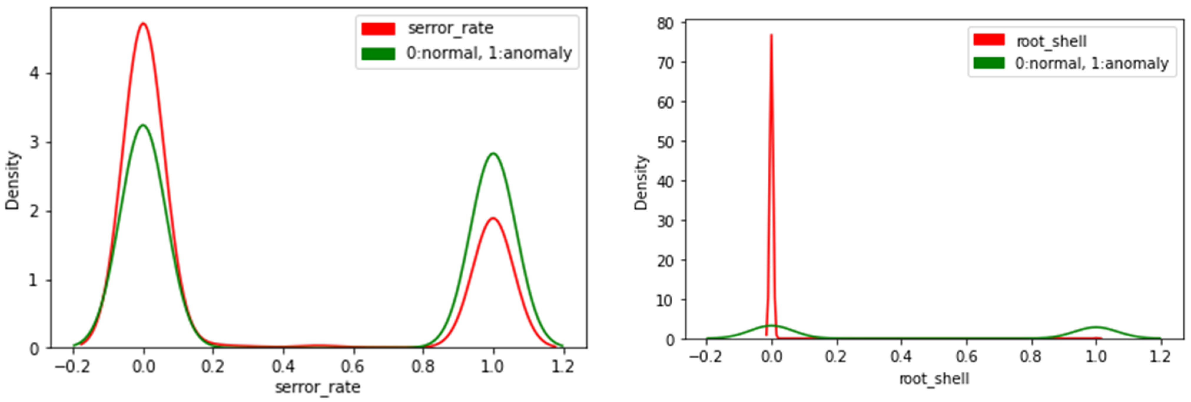
Kernel density distribution can be described as a linear representation of a data histogram; it describes how values are distributed over certain feature values. For example, Figure 2 shows the density distribution for two features, “serror_rate” and “root_shell”. The distribution for the “root_shell” feature shows that values for this feature are distributed around 0. While the value of 80 corresponding to 0 in the “root_shell” figure is a numeric indicator for data distribution, the higher the y-axis value, the denser data are around the corresponding value on the x-axis.

Figure 2. Density function examples.

The data set was split into two datasets: dataset1 (DS1) and dataset2 (DS2). DS1 contains features whose KDE plot showed data tightly concentrated around certain values. DS2 contains the rest of the features with a relaxed KDE plot. DS1 included 19 features, while DS2 contained the other 21 features. The original dataset with the 40 features will be called DS throughout the rest of the study for simplicity.

Dataset classification was undertaken based on the visual realization of the features of the KDE plots. In Table 2, the features and their classification are listed. Each feature type was also listed to indicate the nature of data, whether discrete or continuous. After classifying features according to KDE plots, the three datasets, DS, DS1, and DS2, were used to train the prediction models: Naive Bayes Classifier, Decision Tree, K-Neighbors Classifier, Logistic Regression, and random forest classifier. A CNN built for intrusion detection was trained with the three datasets. The accuracy for each model with DS, DS1, and DS2 was measured and recorded.

Table 2. Dataset classification based on KDE plot.

Feature Name	Type	Dataset
duration	continuous	DS1
protocol_type	symbolic	DS1
Service	symbolic	DS1
src_bytes	continuous	DS1
dst_bytes	continuous	DS1
Flag	symbolic	DS2
Land	symbolic	DS1
wrong_fragment	continuous	DS1
Urgent	continuous	DS1
Hot	continuous	DS1
num_failed_logins	continuous	DS2
logged_in	symbolic	DS2
num_compromised	continuous	DS1
root_shell	continuous	DS1
su_attempted	continuous	DS1
num_root	continuous	DS1
num_file_creations	continuous	DS1
num_shells	continuous	DS1
num_access_files	continuous	DS1
num_outbound_cmds	continuous	DS1
is_hot_login	symbolic	DS1
is_guest_login	symbolic	DS1
Count	continuous	DS2
srv_count	continuous	DS2
serror_rate	continuous	DS2
srv_serror_rate	continuous	DS2
rerror_rate	continuous	DS2
srv_rerror_rate	continuous	DS2
same_srv_rate	continuous	DS2
diff_srv_rate	continuous	DS2
srv_diff_host_rate	continuous	DS2
dst_host_count	continuous	DS2
dst_host_srv_count	continuous	DS2
dst_host_same_srv_rate	continuous	DS2
dst_host_diff_srv_rate	continuous	DS1
dst_host_same_src_port_rate	continuous	DS2
dst_host_srv_diff_host_rate	continuous	DS2
dst_host_serror_rate	continuous	DS2
dst_host_srv_serror_rate	continuous	DS2
dst_host_rerror_rate	continuous	DS2
dst_host_srv_rerror_rate	continuous	DS2

As some models showed a notable change in measured accuracy, the SHAP library was used to detect the most important 20 features of the DS dataset for each model and which model these features mostly belong among DS1 and DS2. Justifying why some features were more efficient than others to a certain ML model was built over the KDE plot of these features. The models’ accuracy was used to measure the model efficiency in identifying the relationship between different features to predict anomalies from normal connections. Accuracy is also used to measure different datasets’ ability to provide useful information for different models.

In this study, the dataset feature analysis based on KDE plots gives deep insight into understanding the amount of information carried in each feature. This information can explain why the model’s performance varies with different datasets, as shown in the next section.

4. Results and Discussion

The results we introduce through this section concern dataset classification, the performance of different models with the datasets, and explaining XAI results for the ML model.

4.1. Dataset Classification

As mentioned earlier, the data set was divided into two non-intersecting datasets. DS2 contains features with a relaxed KDE plot, and DS1 contains features with a KDE plot showing highly dense regions. Highly dense regions indicate that the majority of the feature values lie around a certain same value (symmetry); on the other hand, the relaxed KDE plot indicates that the values of the features are distributed and varied. Table 2 shows how the features were classified according to the visual realization of the KDE plot for each feature.

As mentioned earlier, DS2 contains features with a relaxed KDE diagram, meaning that the values representing these features are spread over their range instead of being gathered within a limited range of values. The classification was undertaken due to visual observation of the features of KDE plots. The KDE plots were generated for the 40 features using the Python seaborn library. The “kdeplot” method (from the seaborn library) was used to generate the KDE plots. The generated plots were realized to be either dense, and most of the feature values are either located in a very limited region of the feature values or distributed over the range of the values in a relaxed shape. Then, the classification process took place based on the KDE plot shape. The classification process resulted in the construction of Table 2 and forming two sub-datasets; DS1, which contains dense features only, and DS2, which contains relaxed features only.

4.2. Performance of ML Classifiers Using Different Datasets

The ML models used in this study were selected due to their frequent usage in training tabular datasets, especially intrusion detection datasets. The selected model’s performance was recently highlighted in the works [44,45,46,47]. ML algorithms are famous and widely used since they can be imported and used easily in Python and provide satisfying results in most cases. The selected ML models’ interpretability was investigated in works such as [48]. The models were imported from python libraries, and no tuning was applied to the used models. In Table 3 below, we mention the model selection criteria. The selected models can all be used with tabular data with no or minor data preprocessing, they can be explained with SHAP and do not require long training and testing time.

Table 3. Machine-learning Algorithms and AI Models Selection Criteria.

Model	Can Be Used with Tabular Data	Can Be Explained with SHAP	Execution Time
Random Forest	YES	YES	Relatively slow
Decision tree	YES	YES	Relatively slow
Naïve Bayes	YES	YES	Fast
Logistic Regression	YES	YES	Fast
CNN	YES	YES	Depends on the architecture used

Figure 3 shows how different ML models performed with the three datasets used in this study and measured via accuracy. “Decision Tree”, “K-Neighbors”, “Logistic regression”, and “random forest” models have shown symmetrical tendencies as they performed almost the same with DS and DS1. The three mentioned models dropped a little accuracy with DS2. While the “Naive Bayes” model and the CNN DS2 notably outperformed DS1.

Figure 3. Validation accuracy for several learning models.

The models’ performances are not compared to each other here; rather, we are trying to find which features are more important to every ML model used and to explain why the feature is important.

This variance in accuracy between DS1 and DS2 can be explained by how these models analyze data and make decisions. A decision tree, for example, relies on data purity to make decisions. The less the data are distributed over a feature, the more it is useful for data classification. In the decision trees, data with low entropy are placed closer to the root and take considerable value in decision-making.

The Naive Bayes algorithm, on the other hand, depends on data probability in each feature. Hence, the features gathered around certain values will provide poor results due to high variance in the probabilities for different values. Values that are less present in a feature will have a probability close to 0, while the other values will have values closer to 1; this pattern of information can be considered inefficient for the model.

CNN works basically by recognizing patterns between different features. According to our estimation, spare values could provide CNN with better feature information. Hence, better results came from DS2. On the other side, distinguishing patterns with dense data was harder for CNNs.

4.3. Explaining XAI Results for the Models

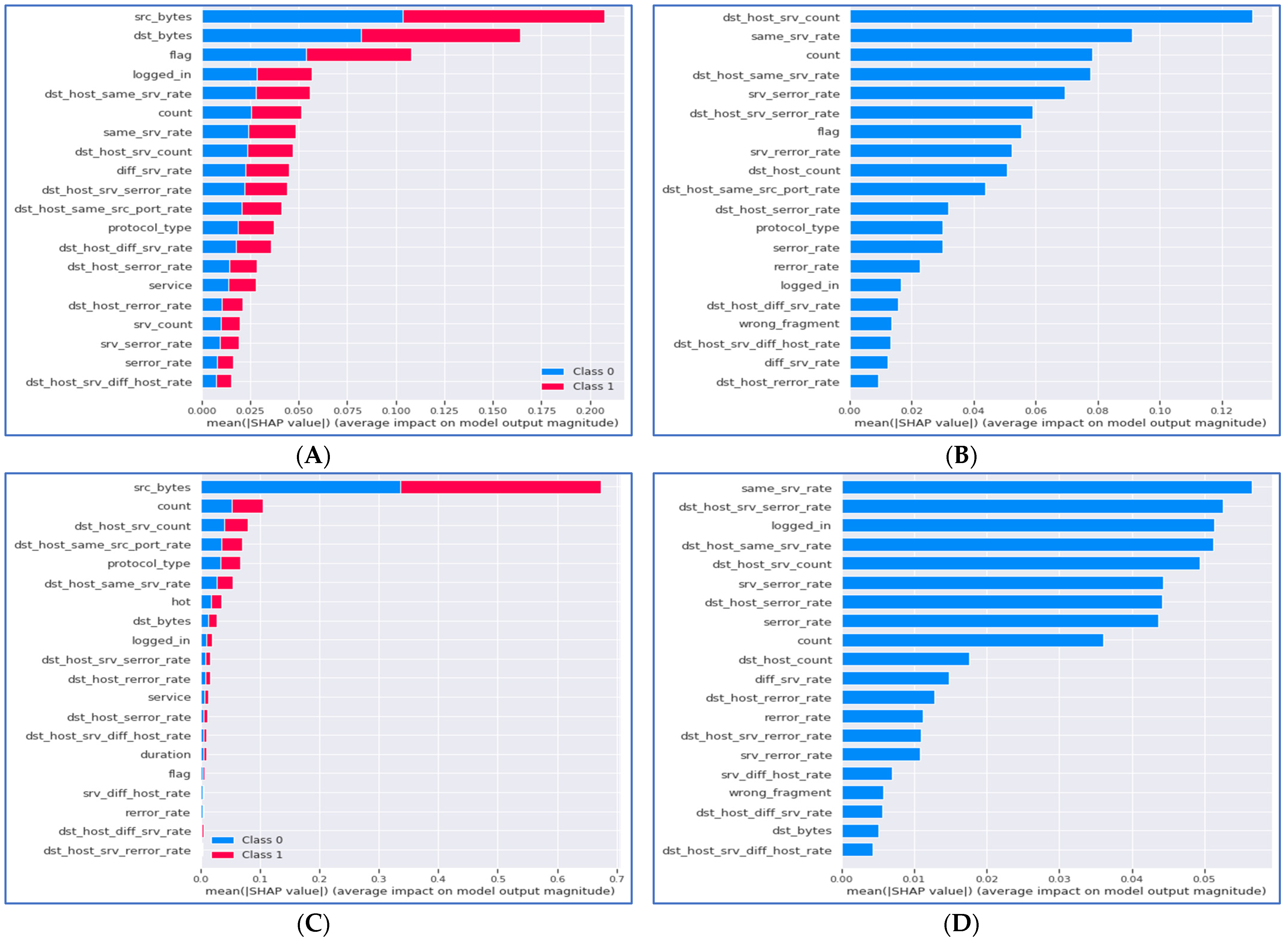
State-of-the-art XAI methods such as SHAP and LIME are used to explain the ML model results. They highlight the names of the features that mostly affected the ML model’s decision. This analysis can be conducted at the level of the single tuple, called local XAI. On the other hand, global XAI provides names of important features for ML models at the level of all tuples used in training the model. We present a global analysis of the ML models mentioned in Figure 4 generated from SHAP libraries.

Figure 4. Global analysis using SHAP for (A) Random Forest Classifier, (B) Logistic Regression Classifier, (C) Decision Tree Classifier, and (D) Naive Bayes Classifier.

Figure 4 shows that the random forest model relies on 11 dense and nine relaxed features. The performance of the random forest model does not vary much between DS, DS1, and DS2 (illustrated in Figure 4A). The reliance on both features makes the model more robust with different data types and reliable with small datasets such as DS1 or DS2. In Figure 4B, the SHAP results for the logistic regression model show that the model mostly relies on dense features. The figure shows that 13 of 20 SHAP important features belong to DS1. This dependency on a certain data type was reflected in the model’s accuracy when trained with DS1 and DS2. Despite this dependency, the model performed better with more features from the DS dataset. The decision tree model showed close to perfect results with the three datasets (illustrated in Figure 4C), a similar behavior to the random forest model. Yet, the SHAP features in Figure 4 are not similar to random forests, and a clear reliance on the feature “src_bytes” is spotted. The Naive Bayes model accuracy results notably varied between DS1 and DS2. The SHAP plot in Figure 4D confirmed the model’s reliance on features belonging to DS2. Such results should be considered when we want to train the Naive Bayes model with a certain dataset. On the other hand, having a data set with features similar to DS2′s Naive Bayes can be recommended as an efficient ML model.

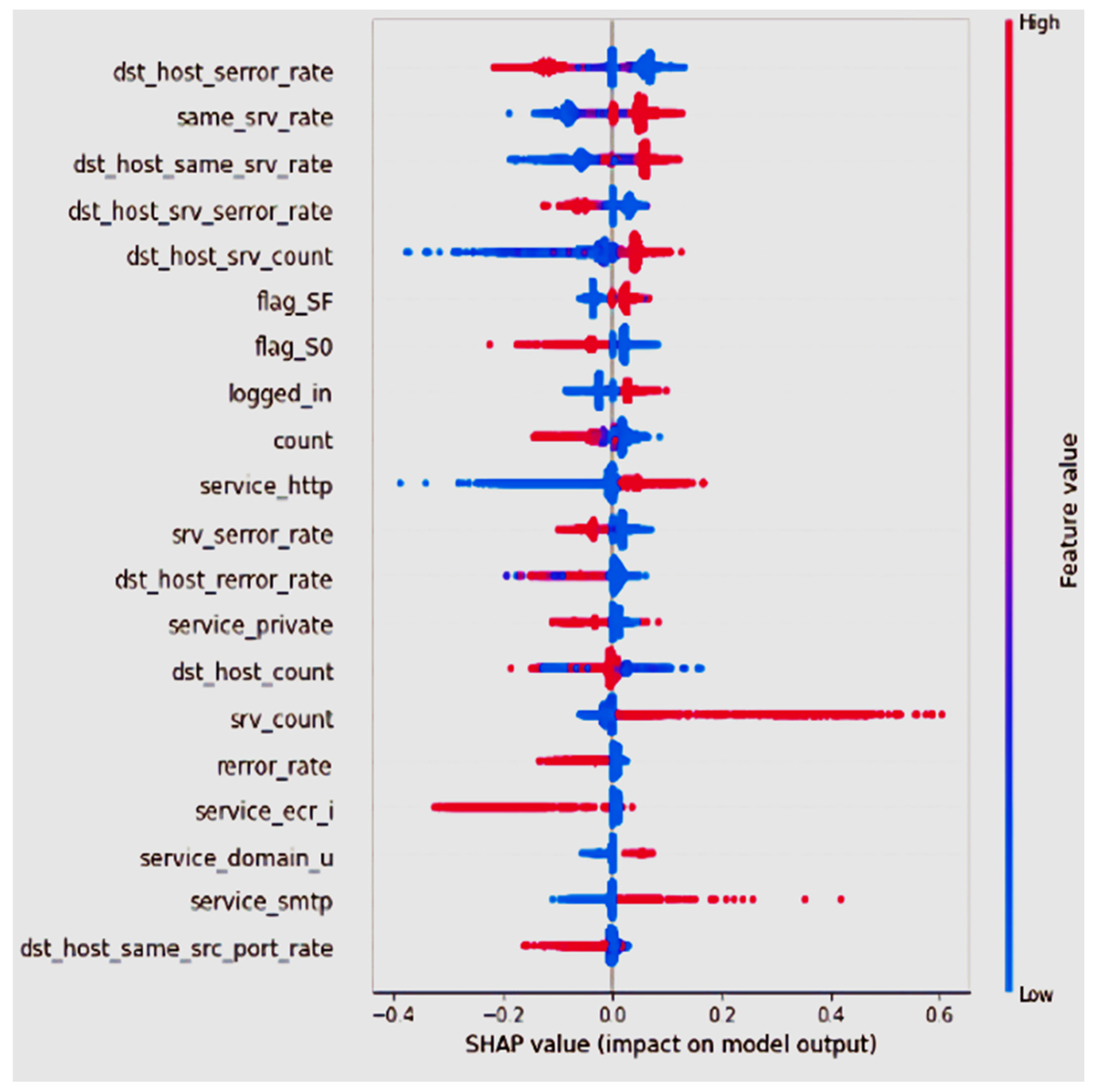
Eventually, we are interested in the XAI results in [36]. We are interested in the results [36] presented and in explaining why the features were considered more or less important to the CNN model. Their work applied the “SHAP” XAI method to the KDD 99 dataset to train a CNN model. The SHAP summary plot they generated is presented in Figure 5. The top 20 important features are listed in the figure. The figure shows that the most important feature is “dst_host_serror_rate”, while the red and blue colors reflect the feature value. Out of the 20 features listed in Figure 5, 14 are included in DS2 of this study.

Figure 5. SHAP Results for KDD Intrusion Detection Dataset Used with A CNN. Courtesy [36].

Figure 5 shows the SHAP summary plot for the AI model presented in [36]; the work presents the XAI model for an intrusion detection system. The AI system in [36] is a neural network that uses the KDD99 dataset to train the AI model. In Figure 5, the authors of [36] present the SHAP global explanation for their model; the SHAP global explanation model presents the global features’ importance. The order of the features is for the important features according to SHAP XAI ordered, such that the most important features are listed at the top of the figure and the least important feature is listed at the bottom. The horizontal values represent the shapely values while the is for the value of the feature from low to high. The red SHAP values increase the prediction, while blue values decrease it.

Additionally, in Figure 6, we present the KDE plot for the two top features listed in Figure 5; the figure shows that the “dst_host_serror_rate” feature has almost the same shape as the “class” feature KDE plot (symmetric). According to the SHAP analysis presented in Figure 5, the low value of the “dst_host_serror_rate” feature increases the predicted anomaly value. On the other hand, a high value for the “same_srv_rate” feature increases the predicted anomaly value. Generally, the KDE plots reflect the shape of the SHAP values, and the most important features belong to features whose KDE plot shape is relaxed.

Figure 6. Top Two Features KDE Plots.

In order to investigate the influence of the features’ distribution shape on their importance in an AI model and confirm the results generated with the KDD99 dataset, we repeated the experiment with a small version of the Kitsune2018 dataset. The distilled-Kitsune2018 [24] includes nine attacks’ data. We used the Mirai attacks dataset to train the machine learning models, while we used Mirai with two other attacks to train the CNN model; Syn DoS and Video injection.

The Mirai dataset consists of 116 features plus the class feature. We plotted the KDE plots of the features and visually classified them into dense and relaxed features. Unlike the KDD99 dataset, the class or the label feature was not balanced; the normal packets were of a larger quantity. We generated the KDE plot for the class feature and each other; then, we classified them into relaxed or dense features. Dense features are features with peaks equal to 14 or higher. These peaks reached around 100 and more values for the extremely dense features. After classifying the features, we found that 40 were relaxed, while the other 76 features were of a dense KDE plot shape.

For the other two attacks listed in Table 4, some features were only added to DS1 and DS2 for each attack. This selection was made since we aimed to study which features are more important to the CNN model, and these features were not equally divided between dense and relaxed features. On the other hand, some features were hard to judge whether they belonged to DS1 or DS2 since human operators make the division visually. Therefore, as shown in Table 4, DS1 and DS2 of the Syn DoS and the Video injection attacks have 23 and 17 features. The features with relaxed KDE plots of DS2 were selected from the features whose KDE plot is similar to the class feature’s KDE plot or conversely following the shape of the KDE plot. These features’ KDE plots are similar to the features in Figure 6.

Table 4. Kitsune2018 Datasets Features.

	Mirai	Syn DoS	Video Injection
Features	116	115	115
Dense (DS1)	76	23	17
Relaxed (DS2)	40	23	17

It should be mentioned here that the distilled-kitsune dataset has no feature names, so we named the features to refer to them. The first feature was given the name “1”, the second one was given the name “2”, and so on. We also changed the labels values from “TRUE” and “FALSE” into “1” and “0” consequently. We trained the four ML models mentioned in Figure 4 with the Kitsune2018 Mirai Attack dataset. Then, we generated the SHAP results for the trained models. The SHAP results were then analyzed to investigate which features are more important to the models.

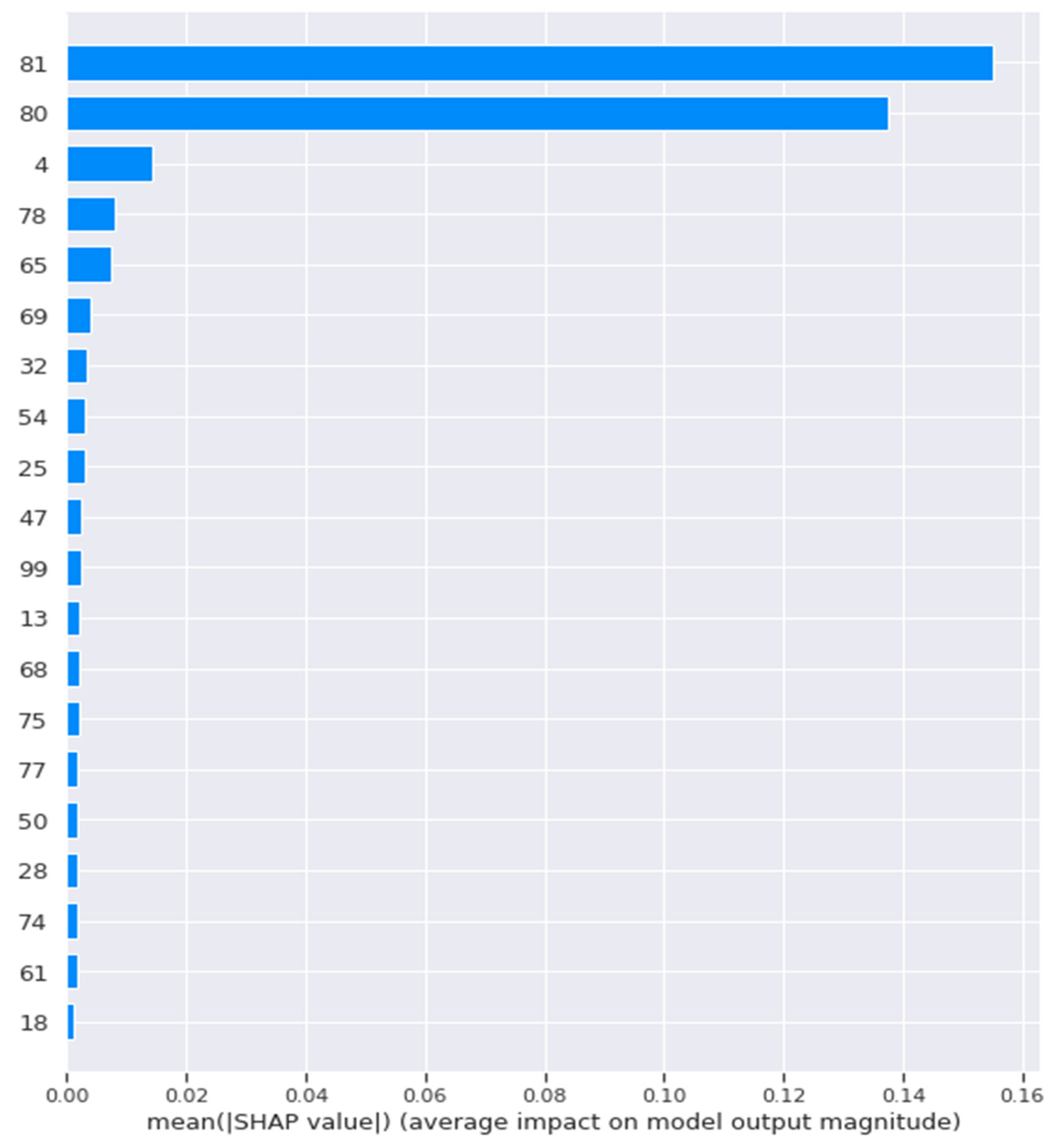
The random forest and the decision tree model achieved similar results; the model’s SHAP results showed that the model mainly relied on 11 relaxed features and nine dense ones. The model achieved accuracy results of 100 when it was trained with the whole dataset, DS1, and DS2 of the Mirai attack dataset. When the Mirai and DS2 of Mirai were used to train the decision tree model, the model relied only on one feature, the most relaxed feature among them all, giving 100% accurate results. When we trained the model with the dense dataset, the SHAP results showed that the model relied on 18 features to achieve the same perfect accuracy, as shown in Figure 7.

Figure 7. SHAP Results for the Decision Tree Model When Dense Features were Used.

Figure 7 represents the SHAP global bar plot; this plot represents the most important features which the model relied on while making its decision; a longer bar indicated a more important feature. This plot shows that the decision tree model used the listed 18 features during decision-making when it was fed with the dense features, features whose numbers are 81 and 80 were highly important compared to the following other 16 features. The global bar plot contained only one feature when the relaxed features were used to train the model, which means that the whole dataset can be replaced with this feature only to achieve 100% accuracy.

No conclusions were built over the Naïve Bays and Logistic Regression since their results were unreliable with the imbalanced datasets. We thought we should not rely on the results to make conclusions. The models could only learn one class, the normal class, which is more dominant in the dataset. Hence, the SHAP results could not be considered since they resulted in totally wrong decisions.

The confusion matrix that was generated when the SynDoS dataset was used with the Naïve Bays model was generated as: “confusion matrix: [[5398 905] [234 462]]”—knowing that the dataset consists of 6999 entries, 6000 normal packets, and 999 anomaly packets. We applied the A\B statistical significance calculations, resulting in a value of 0 for both the tailed p-values and the one-tailed p-value, which means that there is a 100% chance that normal packets have a higher proportion. This statistical analysis led to excluding the Naïve Bayes model from the study when we used the Kitsune2018 dataset. On the other side, the decision tree model can be described as a “confusion matrix: [[6303 0] [0 696]]”. The Two-Tailed p-value, in this case, is 0.8119215, and the one One-Tailed p-value is 0.4059607. This means there is a 59.404% chance that normal has a higher proportion. These calculations were generated using simple programs developed with excel. We considered true positive and negative values in the confusion matrix as the success times for each model.

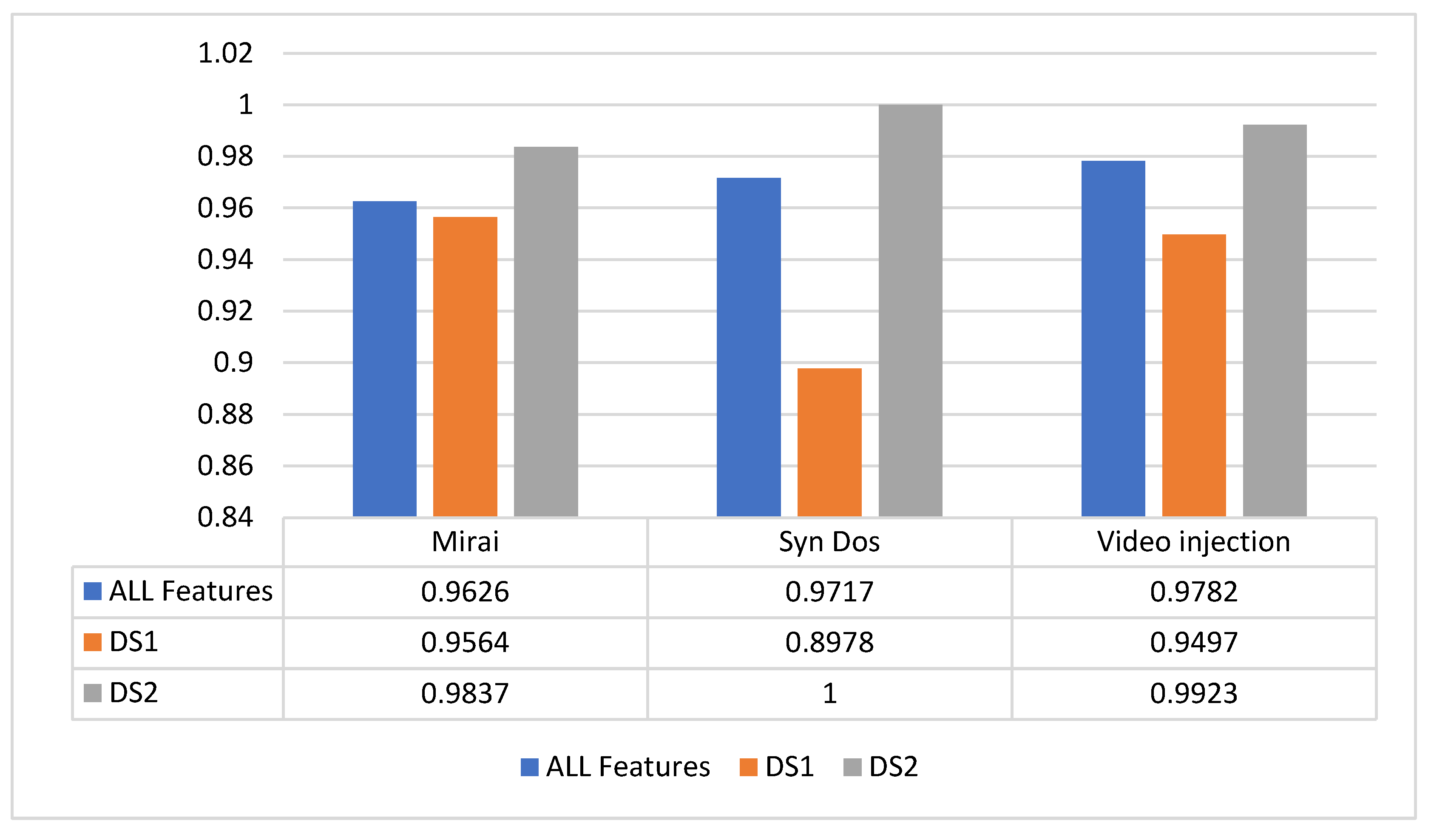
The CNN model was trained with three attack datasets from Kitsune2018. The attacks are the Mirai, the Syn DoS, and the Video injection attacks. The CNN accuracy was higher for the three unbalanced datasets when we used DS2 to train the CNN. As shown in Figure 8, the CNN model accuracy was raised every time it was trained with DS2 and decreased when it was trained with DS1 compared to training the model with all the features in the dataset. Removing the features whose KDE plots are centered around one value was similar to a cleaning process for the datasets and achieved better accuracy results. The Syn DoS DS2, for example, achieved an accuracy of 100% with 23 features only, while training the model with 115 features could not reach an accuracy of 100%. When Syn DoS DS1 was used to train the model, the model was affected by the data imbalance and could only learn the normal class according to the f1-score and recall measurements. This example shows how dense features were not a suitable choice to be used with CNN models. A decision tree or random forest models are more recommended with datasets whose KDE plots are highly dense.

Figure 8. The CNN model results in different datasets and sub-dataset.

The video injection sub-datasets consist of 17 features only, selected from 115 features. Yet, the 17 selected features provided better results than the 115-feature dataset. In the case of using DS2 features only, more accurate results can be achieved in less time and less complicated CNNs.

The KDD99 dataset is a balanced dataset with 40 features and around 25,000 entries; it includes packets of DOS attacks collected in 1999. Around half the features of KDE, plots are of relaxed shape. While on the other hand, the Kitsune dataset, which we used later, includes packets for nine different attacks, most of which are more up-to-date. The used datasets include 115 features and 116 for the Mirai attack. The features are not equally divided into relaxed and dense features. The number of entries for each attack’s dataset is 9999; 9000 are normal, and the rest are anomalies.

The AI and ML models listed in Figure 3 could mostly provide good results with the KDD99 dataset, DS1, and DS2 of KDD99, as clarified in Figure 3. The ML models used 25,000 entries balanced between the two classes, anomaly and normal, to train the model. Usually, intrusion detection datasets are not balanced. Hence, we used another more up-to-date unbalanced dataset of [49] to confirm the results we generated with the KDD99.

Kisune2018 could not reach satisfying results with the logistic regression or the naïve bay model due to the data imbalance; the models expected all the tuples as normal. While the random forest and the decision tree models result for both KDD99 and Kitsune2018 can provide the same conclusions. The random forest can make use of dense and relaxed features. Meanwhile, the decision tree model gives perfect results with relaxed and dense features but can only reach 100% precision using one relaxed feature.

The interesting results came with the CNN model since we relied on the results of [36] to expect that relaxed features whose KDE plots are similar to those listed in Figure 6 can greatly benefit CNN models. The KDD99 CNN experiment was repeated with three attacks from the Kitsune2018 dataset, and it was clear that CNN models could learn from the DS2 datasets more than they could learn from the relaxed features mixed with the dense ones. Removing the dense features can be used as an efficient data-cleaning strategy when CNN models are used. The results shown in Figure 8 can be used to explain and expect CNN models’ performance with different datasets.

Our work is not a solo study focusing on judging and evaluating XAI systems and methods. Our study focused on explaining XAI results and finding shortcuts to customizing proper ML models to a certain dataset. The customization process was built over SHAP results. Other studies, such as [50,51,52], focused on studying the variant XAI method’s performance with different ML models and datasets. The studies were directed toward exploring how and how far these XAI systems can be beneficial in interpreting ML model results. The study presented in [2] answered the question of what we want of XAI as long as AI works efficiently. The answer to the question was that these XAI methods are supposed to help human operators, and individuals standing behind these ML models should have more trust in the generated results, as well as should be provided with an insight into the basis these decisions were taken upon, so prudent decisions would be taken with more strict safety margins. The work presented in [22] analyzed the information provided by different XAI methods and highlighted that XAI methods could explain ML models.

In contrast, they cannot explain themselves and present justifications for why certain features are more important than others. This study is a step forward in covering this gap. The work in [53] presented a scale to evaluate XIA model explanations in human–machine work systems, but they did not provide explanations. Other studies, such as [23], believed that the current XAI models do not satisfy the need to understand how an ML model works internally but rather give a shallow justification of how final results were extracted. We believe in this study that we have presented a method to explain the results of XAI models and methods such as SHAP.

The work of [37] presented seven strategies that might aid in trusting XAI; the first proposed strategy was to create methods to explain the results of XAI, which is what this work has presented. We might consider this work as a state-of-the-art work moving forward toward explaining these results. The fifth mentioned strategy in [24] was to build ML models knowing in advance that the model should provide satisfying results instead of taking chances through selecting a proper ML model; here again, our work is presenting a methodology that can be used with tabular datasets to select a proper ML model. For example, CNN models prefer datasets with features mostly composed of relaxed KDE-shaped feathers to dense ones. In Table 5, we summarize the mentioned works in this section.

Table 5. Summary of other works which evaluated XAI methods and explained them.

Reference	The Contribution to Assessing and Evaluating XAI
[51]	They explored why XAI is important and categorized XAI methods in their scope, methodology, usage, and nature. The study focused on explaining deep neural network algorithms.
[52]	Evaluated trending XAI methods and showed how these methods show the internal layer’s content of ML models.
[2]	Answered the question of what we want from XAI models and answered the question that these models can be more trusted with the aid of XAI.
[22]	Analyzed the information provided by different XAI methods and discussed some inabilities in the current XAI methods.
[53]	Presented a scale to evaluate XIA model explanations in human–machine work systems.
[23]	Discussed some inabilities in the current XAI methods.
[24]	Presented seven strategies that might aid in trusting XAI.
Present Study	Presents a method to explain SHAP results for different ML models based on the KDE plots of the features’ data.

In summary, his work can be considered a state-of-the-artwork suggestion for a new strategy to clean datasets to enhance CNN models’ performance. This work also suggests that the features’ KDE plots can be used as a powerful tool to select the proper model to train a certain dataset. We also confirm that KDE plots can be used to select proper features for CNN models.

The work could explain why and how datasets can benefit different ML models and CNNs based on the features’ KDE plots. In this work, we showed that features KDE plots had presented a deep abstraction for the amount and the nature of the values carried in each feature of the dataset. The KDE plots carried information that was then used to justify the behavior of different ML models with different datasets. The KDE plots were also linked with SHAP results to explain the ML models further. It is speculated that the presented methodology should greatly impact XAI methods such as SHAP.

5. Conclusions and Future Directions

An analytical approach for studying intrusion detection dataset features using density functions has been presented and discussed in this paper. The proposed model study seeks to explain how and why these features are considered important during the XAI process. The proposed model seeks to explain XAI behavior to add an extra layer of Explainability. The density function analysis presented in this paper adds a deeper understanding of the importance of features in different ML models. This work has classified the KDD and Distilled Kitsune-2018 intrusion detection datasets into two non-intersecting subsets based on their KDE function plots. We have studied the accuracy of different ML models with the two subsets and the original dataset. We have found that the sub-dataset that contained non-dense features outperformed the other dataset when used to train an intrusion detection CNN model. We also found that features whose values distribution is similar to the class feature distribution can greatly benefit the CNN model. Removing the other features from the dataset can enhance the model’s accuracy. We have also matched our work with the SHAP XAI results for Multiple ML models and used the KDE plots of the features selected by SHAP to explain why they are more important to a CNN than the others. In the future, we might expand the study into other datasets such as an image or medical image datasets to determine the features or shape of the images KDE plots that can be more useful and achieve better results with CNN models. The study might be expanded to be used with other, more sophisticated deep learning or ensemble models. For example, KDE plots might be generated for images-or objects inside the images- pixels values, and then XAI results for ML models might be justified using these results. Expanding the current work into other forms of data other than tabular data might be a good scope for further research. Automating the separation of the features based on the shape of the KDE plot might be an important advancement to the current work. This might be undertaken by studying the number of peaks inside the KDE plot. The major limitation of this work is the need to classify the features of the used dataset based on the visual observations of their KDE plots. The process can consume a considerable amount of time, and some features might not belong to too dense or relaxed features. In the case when the features’ KDE plots were hard to classify, the features were not used in both groups; this might be limiting in cases when too many features are debatable.

References

1. Abu Al-Haija, Q.; Al-Badawi, A. Attack-Aware IoT Network Traffic Routing Leveraging Ensemble Learning. Sensors 2022, 22, 241. [Google Scholar] [CrossRef] [PubMed]
2. Ring, M.; Wunderlich, S.; Scheuring, D.; Landes, D.; Hotho, A. A Survey of Network-Based Intrusion Detection Data Sets, Computers & Security; Elsevier: Amsterdam, The Netherlands, 2019; Volume 86, pp. 147–167. [Google Scholar]
3. Le, T.-T.-H.; Kim, H.; Kang, H.; Kim, H. Classification and Explanation for Intrusion Detection System Based on Ensemble Trees and SHAP Method. Sensors 2022, 22, 1154. [Google Scholar] [CrossRef]
4. Mahbooba, B.; Timilsina, M.; Sahal, R.; Serrano, M. Explainable artificial intelligence (XAI) to enhance trust management in intrusion detection systems using decision tree model. Complexity 2021, 2021, 6634811. [Google Scholar] [CrossRef]
5. Srinivasu, P.N.; Sandhya, N.; Jhaveri, R.H.; Raut, R. From Blackbox to Explainable AI in Healthcare: Existing Tools and Case Studies. Mob. Inform. Syst. 2022, 2022, 8167821. [Google Scholar] [CrossRef]
6. Abir, W.H.; Uddin, M.; Khanam, F.R.; Tazin, T.; Khan, M.M.; Masud, M.; Aljahdali, S. Explainable AI in Diagnosing and Anticipating Leukemia Using Transfer Learning Method. Comput. Intell. Neurosci. 2022, 2022, 5140148. [Google Scholar] [CrossRef] [PubMed]
7. Dieber, J.; Sabrina, K. Why model why? Assessing the strengths and limitations of LIME. arXiv 2020, arXiv:2012.00093. [Google Scholar]
8. Neupane, S.; Ables, J.; Anderson, W.; Mittal, S.; Rahimi, S.; Banicescu, I.; Seale, M. Explainable Intrusion Detection Systems (X-IDS): A Survey of Current Methods, Challenges, and Opportunities. arXiv 2022, arXiv:2207.06236. [Google Scholar]
9. Islam, S.R.; Eberle, W.; Ghafoor, S.K.; Ahmed, M. Explainable artificial intelligence approaches: A survey. arXiv 2021, arXiv:2101.09429. [Google Scholar]
10. Alahmed, S.; Alasad, Q.; Hammood, M.M.; Yuan, J.-S.; Alawad, M. Mitigation of Black-Box Attacks on Intrusion Detection Systems-Based ML. Computers 2022, 11, 115. [Google Scholar] [CrossRef]
11. Gramegna, A.; Giudici, P. SHAP and LIME: An evaluation of discriminative power in credit risk. Front. Artif. Intell. 2021, 4, 752558. [Google Scholar] [CrossRef]
12. Jesus, S.; Belém, C.; Balayan, V.; Bento, J.; Saleiro, P.; Bizarro, P.; Gama, J. How can I choose an explainer? An application-grounded evaluation of post-hoc explanations. In Proceedings of the 2021 ACM Conference on Fairness, Accountability, and Transparency, Virtual Event Canada, 3–10 March 2021; pp. 805–815. [Google Scholar]
13. Zhang, C.A.; Cho, S.; Vasarhelyi, M. Explainable Artificial Intelligence (XAI) in auditing. Int. J. Account. Inf. Syst. 2022, 46, 100572. [Google Scholar] [CrossRef]
14. Gunning, D.; Stefik, M.; Choi, J.; Miller, T.; Stumpf, S.; Yang, G.Z. XAI—Explainable artificial intelligence. Sci. Robot. 2019, 4, eaay7120. [Google Scholar] [CrossRef] [PubMed]
15. Lundberg, S. An Introduction to Explainable AI with Shapley Values. Revision 45b85c18. 2018. Available online: https://shap.readthedocs.io/en/latest/overviews.html (accessed on 1 June 2022).
16. Ribeiro, M.T. Local Interpretable Model-Agnostic Explanations (Lime). Revision 533368b7. 2016. Available online: https://lime-ml.readthedocs.io/en/latest/ (accessed on 22 May 2022).
17. Ahmed, I.; Kumara, I.; Reshadat, V.; Kayes, A.S.M.; van den Heuvel, W.-J.; Tamburri, D.A. Travel Time Prediction and Explanation with Spatio-Temporal Features: A Comparative Study. Electronics 2022, 11, 106. [Google Scholar] [CrossRef]
18. Velmurugan, M.; Ouyang, C.; Moreira, C.; Sindhgatta, R. Evaluating Fidelity of Explainable Methods for Predictive Process Analytics. In Intelligent Information Systems; Nurcan, S., Korthaus, A., Eds.; Springer: Cham, Switzerland, 2021; Volume 424. [Google Scholar] [CrossRef]
19. Kumara, I.; Ariz, M.H.; Chhetri, M.B.; Mohammadi, M.; van Den Heuvel, W.-J.; Tamburri, D.A. FOCloud: Feature Model Guided Performance Prediction and Explanation for Deployment Configurable Cloud Applications. In Proceedings of the 2022 IEEE World Congress on Services (SERVICES), Barcelona, Spain, 10–16 July 2022. [Google Scholar] [CrossRef]
20. Roberts, C.V.; Ehtsham, E.; Ashok, C. On the Bias-Variance Characteristics of LIME and SHAP in High Sparsity Movie Recommendation Explanation Tasks. arXiv 2022, arXiv:2206.04784. [Google Scholar]
21. Panati, C.; Wagner, S.; Brüggenwirth, S. Feature Relevance Evaluation using Grad-CAM, LIME and SHAP for Deep Learning SAR Data Classification. In Proceedings of the 2022 23rd International Radar Symposium (IRS), Gdansk, Poland, 12–14 September 2022; IEEE: Piscataway, NJ, USA, 2022; pp. 457–462. [Google Scholar]
22. Brent, M.; Chris, R.; Sandra, W. Explaining Explanations in AI. In Proceedings of the Conference on Fairness, Accountability, and Transparency (FAT* ’19), Atlanta, GA, USA, 29–31 January 2019; Association for Computing Machinery: New York, NY, USA, 2019; pp. 279–288. [Google Scholar] [CrossRef]
23. Páez, A. The Pragmatic Turn in Explainable Artificial Intelligence (XAI). Minds Mach. 2019, 29, 441–459. [Google Scholar] [CrossRef]
24. de Bruijn, H.; Warnier, M.; Janssen, M. The perils and pitfalls of explainable AI: Strategies for explaining algorithmic decision-making. Gov. Inf. Q. 2022, 39, 101666. [Google Scholar] [CrossRef]
25. Houda, Z.A.E.; Brik, B.; Khoukhi, L. Why Should I Trust Your IDS?: An Explainable Deep Learning Framework for Intrusion Detection Systems in the Internet of Things Networks. IEEE Open J. Commun. Soc. 2022, 3, 1164–1176. [Google Scholar] [CrossRef]
26. O’Kane, P.; Sezer, S.; McLaughlin, K.; Im, E.G. SVM Training Phase Reduction Using Dataset Feature Filtering for Malware Detection. IEEE Trans. Inf. Forensics Secur. 2013, 8, 500–509. [Google Scholar] [CrossRef][Green Version]
27. Itani, S.; Lecron, F.; Fortemps, P. A one-class classification decision tree based on kernel density estimation. Appl. Soft Comput. 2020, 91, 106250. [Google Scholar] [CrossRef]
28. Zebin, T.; Rezvy, S.; Luo, Y. An Explainable AI-Based Intrusion Detection System for DNS over HTTPS (DoH) Attacks. IEEE Trans. Inf. Forensics Secur. 2022, 17, 2339–2349. [Google Scholar] [CrossRef]
29. Syed, W.; Irfan, K. Explainable signature-based machine learning approach for identification of faults in grid-connected photovoltaic systems. arXiv 2021, arXiv:2112.14842. [Google Scholar]
30. Michalopoulos, P. Comparing Explanations for Black-Box Intrusion Detection Systems. Master’s Thesis, Mathematics and Computer Science Department, Eindhoven University of Technology, Eindhoven, The Netherlands, 24 January 2020. [Google Scholar]
31. Schlegel, U.; Arnout, H.; El-Assady, M.; Oelke, D.; Keim, D.A. Towards a rigorous evaluation of Xai methods on time series. In Proceedings of the 2019 IEEE/CVF International Conference on Computer Vision Workshop (ICCVW), Seoul, Korea, 27–28 October 2019; IEEE: Piscataway, NJ, USA; pp. 4197–4201. [Google Scholar]
32. Durán, J.M.; Jongsma, K.R. Who is afraid of black box algorithms? On the epistemological and ethical basis of trust in medical AI. J. Med. Ethics 2021, 47, 329–335. [Google Scholar] [CrossRef]
33. Khedkar, S.P.; Ramalingam, A.C. Classification and Analysis of Malicious Traffic with Multi-layer Perceptron Model. Ingénierie Syst. d’Inf. 2021, 26, 303–310. [Google Scholar] [CrossRef]
34. Abuomar, O.; Sogbe, P. Classification and Detection of Chronic Kidney Disease (CKD) Using Machine Learning Algorithms. In Proceedings of the 2021 International Conference on Electrical, Computer and Energy Technologies (ICECET), Cape Town, South Africa, 9–10 December 2021; IEEE: Piscataway, NJ, USA, 2021; pp. 1–8. [Google Scholar] [CrossRef]
35. Hasan, M.J.; Sohaib, M.; Kim, J.M. An Explainable AI-Based Fault Diagnosis Model for Bearings. Sensors 2021, 21, 4070. [Google Scholar] [CrossRef]
36. Shraddha, M.; Dattaraj, R. Explaining Network Intrusion Detection System Using Explainable AI Framework. arXiv 2021, arXiv:2103.07110. [Google Scholar]
37. Dang, Q.-V. Improving the performance of the intrusion detection systems by the machine learning explainability. Int. J. Web Inf. Syst. 2021, 17, 537–555. [Google Scholar] [CrossRef]
38. Devarakonda, A.; Sharma, N.; Saha, P.; Ramya, S. Network intrusion detection: A comparative study of four classifiers using the NSL-KDD and KDD’99 datasets. J. Physics: Conf. Ser. 2022, 2161, 012043. [Google Scholar] [CrossRef]
39. Zhang, C.; Jia, D.; Wang, L.; Wang, W.; Liu, F.; Yang, A. Comparative Research on Network Intrusion Detection Methods Based on Machine Learning. Comput. Secur. 2022, 121, 102861. [Google Scholar] [CrossRef]
40. Abu Al-Haija, Q.; Zein-Sabatto, S. An Efficient Deep-Learning-Based Detection and Classification System for Cyber-Attacks in IoT Communication Networks. Electronics 2020, 9, 2152. [Google Scholar] [CrossRef]
41. Sathianarayanan, B.; Singh Samant, Y.C.; Conjeepuram Guruprasad, P.S.; Hariharan, V.B.; Manickam, N.D. Feature-based augmentation and classification for tabular data. CAAI Trans. Intell. Technol. 2022, 7, 481–491. [Google Scholar] [CrossRef]
42. Ahsan, H. A Study on How Data Quality Influences Machine Learning Predictability and Interpretability for Tabular Data. Ph.D. Dissertation, Youngstown State University, Youngstown, OH, USA, 2022. [Google Scholar]
43. Montavon, G.; Kauffmann, J.; Samek, W.; Müller, K.R. Explaining the Predictions of Unsupervised Learning Models. In xxAI—Beyond Explainable AI; Holzinger, A., Goebel, R., Fong, R., Moon, T., Müller, K.R., Samek, W., Eds.; Springer: Cham, Switzerland, 2022; Volume 13200. [Google Scholar] [CrossRef]
44. Patil, S.; Varadarajan, V.; Mazhar, S.M.; Sahibzada, A.; Ahmed, N.; Sinha, O.; Kumar, S.; Shaw, K.; Kotecha, K. Explainable Artificial Intelligence for Intrusion Detection System. Electronics 2022, 11, 3079. [Google Scholar] [CrossRef]
45. Hussein, M.A. Performance Analysis of different Machine Learning Models for Intrusion Detection Systems. J. Eng. 2022, 28, 61–91. [Google Scholar]
46. Rawat, S.; Srinivasan, A.; Ravi, V.; Ghosh, U. Intrusion detection systems using classical machine learning techniques vs. integrated unsupervised feature learning and deep neural network. Int. Technol. Lett. 2022, 5, e232. [Google Scholar] [CrossRef]
47. Bertoli, G.D.C.; Junior, L.A.P.; Saotome, O.; Dos Santos, A.L.; Verri, F.A.N.; Marcondes, C.A.C.; Barbieri, S.; Rodrigues, M.S.; De Oliveira, J.M.P. An End-to-End Framework for Machine Learning-Based Network Intrusion Detection System. IEEE Access 2021, 9, 106790–106805. [Google Scholar] [CrossRef]
48. Mahbooba, B.; Sahal, R.; Alosaimi, W.; Serrano, M. Trust in intrusion detection systems: An investigation of performance analysis for machine learning and deep learning models. Complexity 2021, 2021, 5538896. [Google Scholar] [CrossRef]
49. Yahalom, R.; Steren, A.; Nameri, Y.; Roytman, M. Small Versions of the Extracted Features Datasets for 9 Attacks on IP Camera and IoT Networks Generated by Mirskey et al., Mendeley Data. 2018. Available online: https://data.mendeley.com/datasets/zvsk3k9cf2/1 (accessed on 1 December 2021).
50. Arrieta, A.B.; Díaz-Rodríguez, N.; Del Ser, J.; Bennetot, A.; Tabik, S.; Barbado, A.; García, S.; Gil-López, S.; Molina, D.; Benjamins, R.; et al. Explainable Artificial Intelligence (XAI): Concepts, taxonomies, opportunities, and challenges toward responsible AI. Inf. Fusion 2020, 58, 82–115. [Google Scholar] [CrossRef]
51. Das, A.; Paul, R. Opportunities and challenges in explainable artificial intelligence (XAI): A survey. arXiv 2020, arXiv:2006.11371. [Google Scholar]
52. Adadi, A.; Mohammed, B. Peeking inside the black-box: A survey on explainable artificial intelligence (XAI). IEEE Access 2018, 6, 52138–52160. [Google Scholar] [CrossRef]
53. Hoffman, R.R.; Klein, G.; Mueller, S.T. Explaining explanation for “explainable AI”. Proc. Hum. Factors Ergon. Soc. Annu. Meet. 2018, 62, 197–201. [Google Scholar] [CrossRef]
Publisher’s Note: MDPI stays neutral with regard to jurisdictional claims in published maps and institutional affiliations.
Article Metrics
Citations
Article Access Statistics
Multiple requests from the same IP address are counted as one view.