
PCB Component Detection Using Computer Vision for Hardware Assurance


 , ,
, , 
Abstract
:1. Introduction
2. Related Works
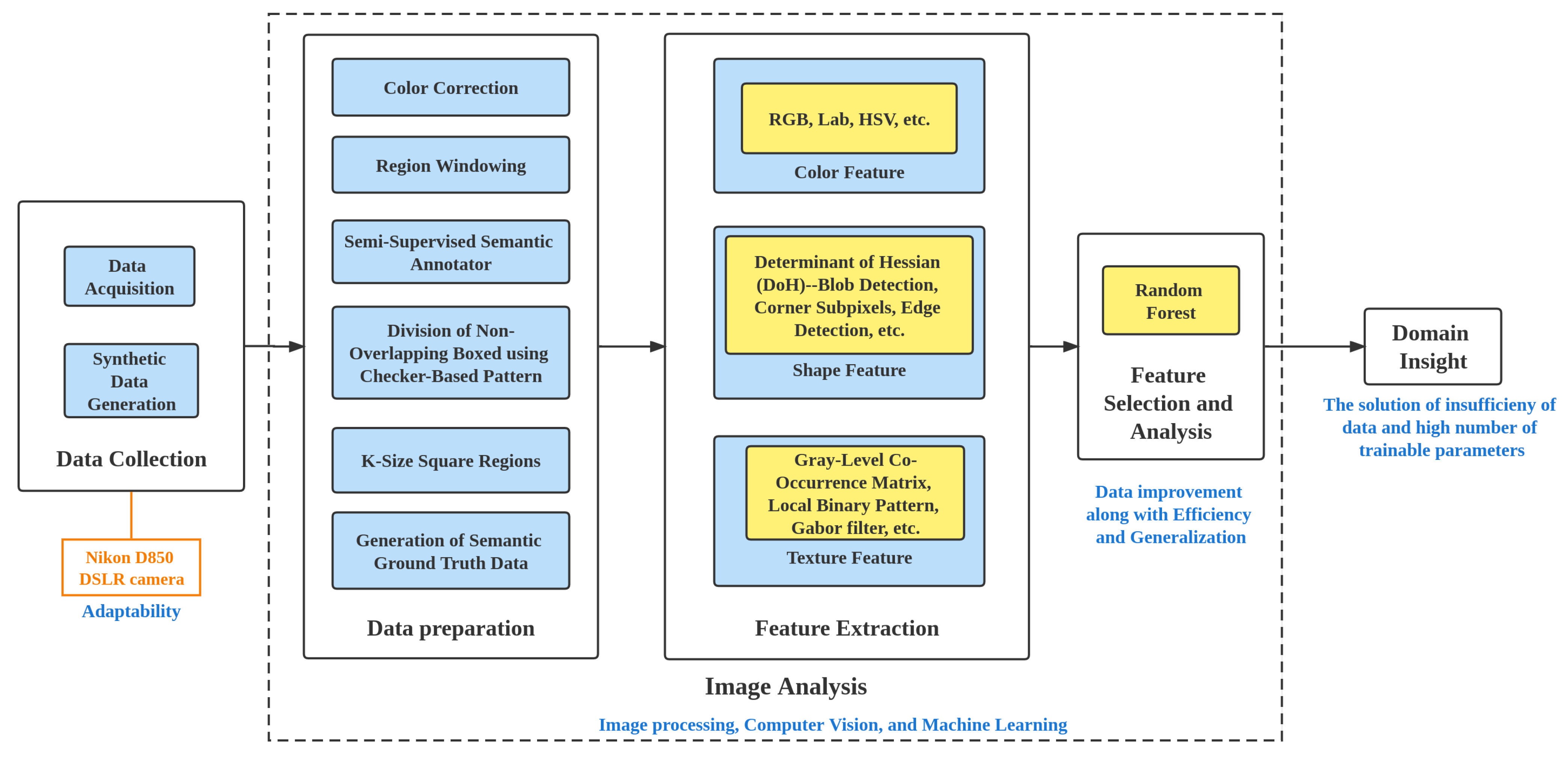
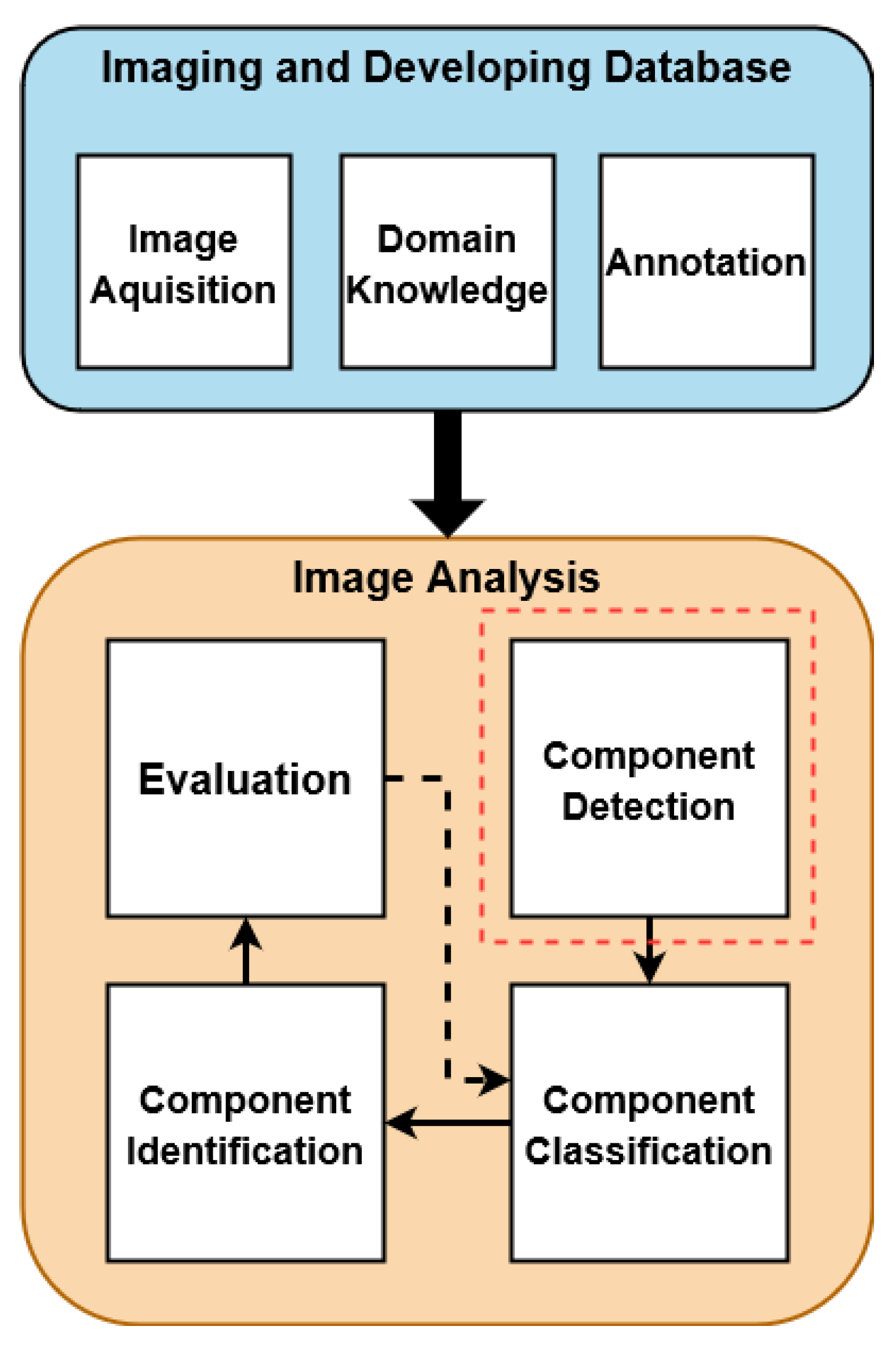
3. Methodology
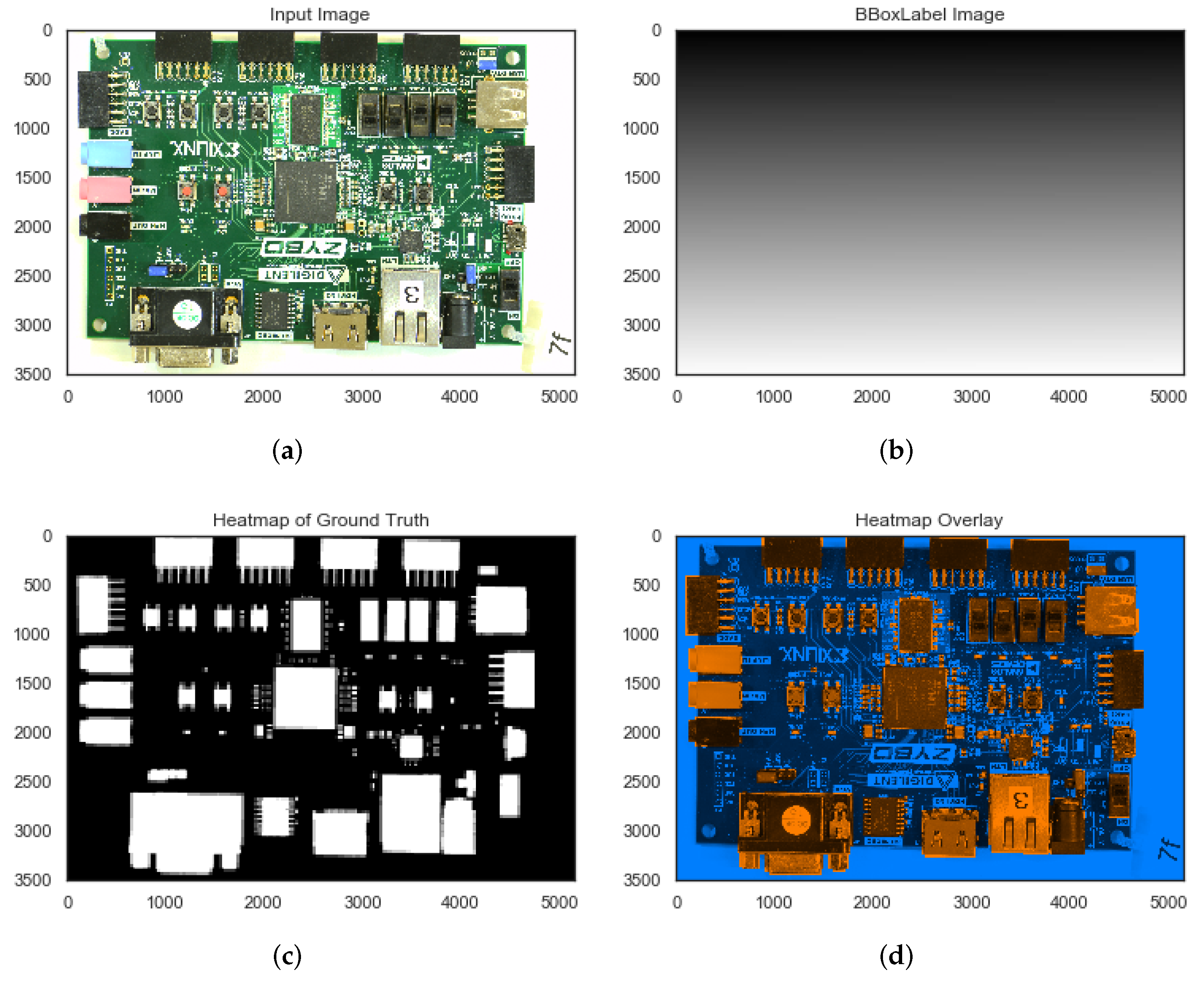
3.1. Data
3.2. Feature Extraction
3.3. Feature Selection and Analysis
4. Color Features
4.1. RGB
4.1.1. Benefits
4.1.2. Limitations
4.2. HSV
4.2.1. Benefits
4.2.2. Limitations
4.3. Lab
4.3.1. Benefits
4.3.2. Limitations
5. Shape Features
5.1. Determinant of Hessian (DoH)–Blob Detection
5.1.1. Hyperparameters
5.1.2. Benefits
5.1.3. Limitations
5.2. Corner Subpixels
5.2.1. Hyperparameters
5.2.2. Benefits
5.2.3. Limitations
5.3. Edge Detection
5.3.1. Hyperparameters
5.3.2. Benefits
5.3.3. Limitations
6. Texture Features
6.1. Gabor Filter
6.1.1. Hyperparameters
6.1.2. Benefits
6.1.3. Limitations
6.2. Gray-Level Co-Occurrence Matrix
6.2.1. Hyperparameters
6.2.2. Benefits
6.2.3. Limitations
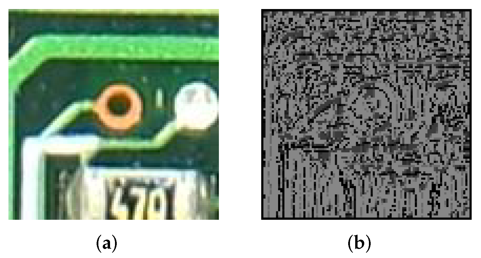
6.3. Local Binary Pattern
6.3.1. Hyperparameters
6.3.2. Benefits
6.3.3. Limitations
7. Results
8. Discussion
9. Conclusions
Author Contributions
Funding
Institutional Review Board Statement
Informed Consent Statement
Data Availability Statement
Acknowledgments
Conflicts of Interest
References
- Lu, H.; Mehta, D.; Paradis, O.P.; Asadizanjani, N.; Tehranipoor, M.; Woodard, D. FICS-PCB: A Multi-Modal Image Dataset for Automated Printed Circuit Board Visual Inspection. IACR Cryptol. ePrint Arch. 2020, 2020, 366. [Google Scholar]
- Mehta, D.; Lu, H.; Paradis, O.P.; MS, M.A.; Rahman, M.T.; Iskander, Y.; Chawla, P.; Woodard, D.L.; Tehranipoor, M.; Asadizanjani, N. The Big Hack Explained: Detection and Prevention of PCB Supply Chain Implants. J. Emerg. Technol. Comput. Syst. 2020, 16, 1–25. [Google Scholar] [CrossRef]
- Paradis, O.P.; Jessurun, N.T.; Tehranipoor, M.; Asadizanjani, N. Color normalization for robust automatic bill of materials generation and visual inspection of PCBs. In Proceedings of the ISTFA 2020, ASM International, Pasadena, CA, USA, 15–19 November 2020; pp. 172–179. [Google Scholar]
- Botero, U.J.; Wilson, R.; Lu, H.; Rahman, M.T.; Mallaiyan, M.A.; Ganji, F.; Asadizanjani, N.; Tehranipoor, M.M.; Woodard, D.L.; Forte, D. Hardware Trust and Assurance through Reverse Engineering: A Tutorial and Outlook from Image Analysis and Machine Learning Perspectives. J. Emerg. Technol. Comput. Syst. 2021, 17, 1–53. [Google Scholar] [CrossRef]
- Zhao, Z.-Q.; Zheng, P.; Xu, S.-T.; Wu, X. Object Detection With Deep Learning: A Review. IEEE Trans. Neural Netw. Learn. Syst. 2019, 30, 3212–3232. [Google Scholar] [CrossRef] [PubMed] [Green Version]
- Sun, Z.; Bebis, G.; Miller, R. Object detection using feature subset selection. Pattern Recognit. 2004, 37, 2165–2176. [Google Scholar] [CrossRef]
- Jović, A.; Brkić, K.; Bogunović, N. A review of feature selection methods with applications. In Proceedings of the 2015 38th International Convention on Information and Communication Technology, Electronics and Microelectronics (MIPRO), Opatija, Croatia, 25–29 May 2015; pp. 1200–1205. [Google Scholar] [CrossRef]
- Geirhos, R.; Rubisch, P.; Michaelis, C.; Bethge, M.; Wichmann, F.; Brendel, W. ImageNet-trained CNNs are biased towards texture; increasing shape bias improves accuracy and robustness. arXiv 2019, arXiv:1811.12231. [Google Scholar]
- Khan, F.; Anwer, R.M.; van de Weijer, J.; Bagdanov, A.D.; Vanrell, M.; López, A.M. Color attributes for object detection. In Proceedings of the 2012 IEEE Conference on Computer Vision and Pattern Recognition, Providence, RI, USA, 16–21 June 2012; pp. 3306–3313. [Google Scholar]
- Diplaros, A.; Gevers, T.; Patras, I. Combining color and shape information for illumination-viewpoint invariant object recognition. IEEE Trans. Image Process. 2006, 15, 1–11. [Google Scholar] [CrossRef]
- Bansal, M.; Kumar, M.; Kumar, M. 2D Object Recognition Techniques: State-of-the-Art Work. Arch. Comput. Methods Eng. 2020, 28, 1147–1161. [Google Scholar] [CrossRef]
- O’Mahony, N.; Campbell, S.; Carvalho, A.; Harapanahalli, S.; Hernandez, G.V.; Krpalkova, L.; Riordan, D.; Walsh, J. Deep Learning vs. Traditional Computer Vision. In Proceedings of the 2019 Computer Vision Conference (CVC), Las Vegas, NV, USA, 2–3 May 2020; pp. 128–144. [Google Scholar]
- Li, J.; Cheng, K.; Wang, S.; Morstatter, F.; Trevino, R.P.; Tang, J.; Liu, H. Feature Selection: A Data Perspective. ACM Comput. Surv. 2017, 50, 1–45. [Google Scholar] [CrossRef]
- Chen, C.H. Handbook of Pattern Recognition and Computer Vision; World Scientific: Singapore, 2015. [Google Scholar]
- Duda, R.O.; Hart, P.E.; Stork, D.G. Pattern Classification and Scene Analysis; Wiley: New York, NY, USA, 1973; Volume 3. [Google Scholar]
- Guyon, I.; Elisseeff, A. An introduction to variable and feature selection. J. Mach. Learn. Res. 2003, 3, 1157–1182. [Google Scholar]
- Liu, H.; Motoda, H. Feature Selection for Knowledge Discovery and Data Mining; Springer Science & Business Media: Cham, Switzerland, 2012; Volume 454. [Google Scholar]
- Kononenko, I. Estimating attributes: Analysis and extensions of RELIEF. In Proceedings of the European Conference on Machine Learning, Catania, Italy, 6–8 April 1994; pp. 171–182. [Google Scholar]
- Ma, L.; Fan, S. CURE-SMOTE algorithm and hybrid algorithm for feature selection and parameter optimization based on random forests. BMC Bioinform. 2017, 18, 169. [Google Scholar] [CrossRef] [PubMed] [Green Version]
- Raschka, S. Python Machine Learning; Packt Publishing Ltd.: Birmingham, UK, 2015. [Google Scholar]
- Breiman, L. Random forests. Mach. Learn. 2001, 45, 5–32. [Google Scholar] [CrossRef] [Green Version]
- Pitas, I. Digital Image Processing Algorithms and Applications; John Wiley & Sons: New York, NY, USA, 2000. [Google Scholar]
- Martínez, J.; Pérez-Ocón, F.; García-Beltrán, A.; Hita, E. Mathematical determination of the numerical data corresponding to the color-matching functions of three real observers using the RGB CIE-1931 primary system and a new system of unreal primaries X’ Y’ Z’. Color Res. Appl. 2003, 28, 89–95. [Google Scholar] [CrossRef] [Green Version]
- Wen, C.Y.; Chou, C.M. Color image models and its applications to document examination. Forensic Sci. J. 2004, 3, 23–32. [Google Scholar]
- Setiawan, N.A.; Seok-Ju, H.; Jang-Woon, K.; Chil-Woo, L. Gaussian mixture model in improved hls color space for human silhouette extraction. In Proceedings of the International Conference on Artificial Reality and Telexistence, Hangzhou, China, 29 November–1 December 2006; pp. 732–741. [Google Scholar]
- Chavolla, E.; Zaldivar, D.; Cuevas, E.; Perez, M.A. Color spaces advantages and disadvantages in image color clustering segmentation. In Advances in Soft Computing and Machine Learning in Image Processing; Springer: Cham, Switzerland, 2018; pp. 3–22. [Google Scholar]
- Kekre, H.; Thepade, S.; Sanas, S. Improving performance of multileveled BTC based CBIR using sundry color spaces. Int. J. Image Process. 2010, 4, 620–630. [Google Scholar]
- El Baf, F.; Bouwmans, T.; Vachon, B. A fuzzy approach for background subtraction. In Proceedings of the 2008 15th IEEE International Conference on Image Processing, San Diego, CA, USA, 12–15 October 2008; pp. 2648–2651. [Google Scholar]
- Sahdra, G.S.; Kailey, K.S. Detection of Contaminants in Cotton by using YDbDr color space. Int. J. Comput. Technol. Appl. 2012, 3, 1118–1124. [Google Scholar]
- Campadelli, P.; Lanzarotti, R.; Lipori, G.; Salvi, E. Face and facial feature localization. In Proceedings of the International Conference on Image Analysis and Processing, Cagliari, Italy, 6–8 September 2005; pp. 1002–1009. [Google Scholar]
- Kekre, H.; Sonawane, K. Comparative study of color histogram based bins approach in RGB, XYZ, Kekre’s LXY and L’ X’ Y’ color spaces. In Proceedings of the 2014 International Conference on Circuits, Systems, Communication and Information Technology Applications (CSCITA), Mumbai, India, 4–5 April 2014; pp. 364–369. [Google Scholar]
- Liu, Z.; Liu, C. A hybrid color and frequency features method for face recognition. IEEE Trans. Image Process. 2008, 17, 1975–1980. [Google Scholar]
- Sudhir, R.; Baboo, L.D.S.S. An efficient CBIR technique with YUV color space and texture features. Comput. Eng. Intell. Syst. 2011, 2, 85–95. [Google Scholar]
- Birchfield, S. Color, in Image Processing and Analysis, 1st ed.; Cengage Learning: Boston, MA, USA, 2018; pp. 401–442. [Google Scholar]
- Smith, A.R. Color gamut transform pairs. ACM Siggraph Comput. Graph. 1978, 12, 12–19. [Google Scholar] [CrossRef]
- Ibraheem, N.A.; Hasan, M.M.; Khan, R.Z.; Mishra, P.K. Understanding color models: A review. ARPN J. Sci. Technol. 2012, 2, 265–275. [Google Scholar]
- Dalal, N.; Triggs, B. Histograms of oriented gradients for human detection. In Proceedings of the 2005 IEEE Computer Society Conference on Computer Vision and Pattern Recognition (CVPR’05), San Diego, CA, USA, 20–25 June 2005; Volume 1, pp. 886–893. [Google Scholar] [CrossRef] [Green Version]
- Lowe, D. Object recognition from local scale-invariant features. In Proceedings of the Proceedings of the Seventh IEEE International Conference on Computer Vision, Kerkyra, Greece, 20–27 September 1999; Volume 2, pp. 1150–1157. [Google Scholar] [CrossRef]
- Rublee, E.; Rabaud, V.; Konolige, K.; Bradski, G. ORB: An efficient alternative to SIFT or SURF. In Proceedings of the IEEE International Conference on Computer Vision, Barcelona, Spain, 6–13 November 2011; pp. 2564–2571. [Google Scholar] [CrossRef]
- Duda, R.O.; Hart, P.E. Use of the Hough Transformation to Detect Lines and Curves in Pictures. Commun. ACM 1972, 15, 11–15. [Google Scholar] [CrossRef]
- Lindeberg, T. Image Matching Using Generalized Scale-Space Interest Points. In Proceedings of the International Conference on Scale Space and Variational Methods in Computer Vision, Leibnitz, Austria, 2–6 June 2013; pp. 355–367. [Google Scholar]
- Zheng, Y.; Meng, F.; Liu, J.; Guo, B.; Song, Y.; Zhang, X.; Wang, L. Fourier transform to group feature on generated coarser contours for fast 2D shape matching. IEEE Access 2020, 8, 90141–90152. [Google Scholar] [CrossRef]
- Häfner, M.; Uhl, A.; Wimmer, G. A novel shape feature descriptor for the classification of polyps in HD colonoscopy. In Proceedings of the International MICCAI Workshop on Medical Computer Vision, Nagoya, Japan, 26 September 2013; pp. 205–213. [Google Scholar]
- Lucchese, L.; Mitra, S.K. Using saddle points for subpixel feature detection in camera calibration targets. In Proceedings of the Asia-Pacific Conference on Circuits and Systems, Denpasar, Indonesia, 28–31 October 2002; Volume 2, pp. 191–195. [Google Scholar]
- Brieu, N.; Schmidt, G. Learning size adaptive local maxima selection for robust nuclei detection in histopathology images. In Proceedings of the 2017 IEEE 14th International Symposium on Biomedical Imaging (ISBI 2017), Melbourne, VIC, Australia, 18–21 April 2017; pp. 937–941. [Google Scholar]
- Canny, J. A computational approach to edge detection. IEEE Trans. Pattern Anal. Mach. Intell. 1986, PAMI-8, 679–698. [Google Scholar] [CrossRef]
- Lowe, D.G. Distinctive Image Features from Scale-Invariant Keypoints. Int. J. Comput. Vis. 2004, 60, 91–110. [Google Scholar] [CrossRef]
- Kenney, C.S.; Zuliani, M.; Manjunath, B.S. An axiomatic approach to corner detection. In Proceedings of the 2005 IEEE Computer Society Conference on Computer Vision and Pattern Recognition (CVPR’05), San Diego, CA, USA, 20–25 June 2005; Volume 1, pp. 191–197. [Google Scholar] [CrossRef] [Green Version]
- Harris, C.; Stephens, M. A combined corner and edge detector. In Proceedings of the Alvey Vision Conference, Manchester, UK, 31 August–2 September 1988. [Google Scholar]
- Shi, J.; Tomasi. Good features to track. In Proceedings of the 1994 Proceedings of IEEE Conference on Computer Vision and Pattern Recognition, Seattle, WA, USA, 21–23 June 1994; pp. 593–600. [Google Scholar] [CrossRef]
- Rong, W.; Li, Z.; Zhang, W.; Sun, L. An improved Canny edge detection algorithm. In Proceedings of the 2014 IEEE International Conference on Mechatronics and Automation, Tianjin, China, 3–6 August 2014; pp. 577–582. [Google Scholar] [CrossRef]
- Abdusalomov, A.; Mukhiddinov, M.; Djuraev, O.; Khamdamov, U.; Whangbo, T.K. Automatic Salient Object Extraction Based on Locally Adaptive Thresholding to Generate Tactile Graphics. Appl. Sci. 2020, 10, 3350. [Google Scholar] [CrossRef]
- Mehrotra, R.; Namuduri, K.; Ranganathan, N. Gabor filter-based edge detection. Pattern Recognit. 1992, 25, 1479–1494. [Google Scholar] [CrossRef]
- Haralick, R.M.; Shanmugam, K.; Dinstein, I. Textural Features for Image Classification. IEEE Trans. Syst. Man, Cybern. 1973, SMC-3, 610–621. [Google Scholar] [CrossRef] [Green Version]
- He, D.C.; Wang, L. Texture Unit, Texture Spectrum, And Texture Analysis. IEEE Trans. Geosci. Remote Sens. 1990, 28, 509–512. [Google Scholar]
- Galloway, M.M. Texture analysis using gray level run lengths. Comput. Graph. Image Process. 1975, 4, 172–179. [Google Scholar] [CrossRef]
- Tamura, H.; Mori, S.; Yamawaki, T. Textural Features Corresponding to Visual Perception. IEEE Trans. Syst. Man Cybern. 1978, 8, 460–473. [Google Scholar] [CrossRef]
- Laws, K.I. Rapid texture identification. In Proceedings of the International Society for Optics and Photonics, SPIE, San Diego, CA, USA, 29 July–1 August 1980; Volume 238, pp. 376–381. [Google Scholar] [CrossRef]
- Baraldi, A.; Panniggiani, F. An investigation of the textural characteristics associated with gray level cooccurrence matrix statistical parameters. IEEE Trans. Geosci. Remote Sens. 1995, 33, 293–304. [Google Scholar] [CrossRef]
- Costa, A.F.; Humpire-Mamani, G.; Traina, A.J.M. An efficient algorithm for fractal analysis of textures. In Proceedings of the 2012 25th SIBGRAPI Conference on Graphics, Patterns and Images, Ouro Preto, Brazil, 22–25 August 2012; pp. 39–46. [Google Scholar] [CrossRef]
- Zhou, J.; Fang, X.; Tao, L. A sparse analysis window for discrete Gabor transform. Circuits Syst. Signal Process. 2017, 36, 4161–4180. [Google Scholar] [CrossRef]
- Stork, D.G.; Wilson, H.R. Do Gabor functions provide appropriate descriptions of visual cortical receptive fields? JOSA A 1990, 7, 1362–1373. [Google Scholar] [CrossRef] [PubMed]
- Pavlovičová, J.; Oravec, M.; Osadský, M. An application of Gabor filters for texture classification. In Proceedings of the ELMAR-2010, Zadar, Croatia, 15–17 September 2010; pp. 23–26. [Google Scholar]
- Teuner, A.; Pichler, O.; Hosticka, B.J. Unsupervised texture segmentation of images using tuned matched Gabor filters. IEEE Trans. Image Process. 1995, 4, 863–870. [Google Scholar] [CrossRef] [PubMed]
- Moraru, L.; Obreja, C.D.; Dey, N.; Ashour, A.S. Dempster-shafer fusion for effective retinal vessels’ diameter measurement. In Soft Computing Based Medical Image Analysis; Elsevier: Amsterdam, The Netherlands, 2018; pp. 149–160. [Google Scholar]
- Öztürk, Ş.; Akdemir, B. Application of feature extraction and classification methods for histopathological image using GLCM, LBP, LBGLCM, GLRLM and SFTA. Procedia Comput. Sci. 2018, 132, 40–46. [Google Scholar] [CrossRef]
- Zhang, X.; Cui, J.; Wang, W.; Lin, C. A study for texture feature extraction of high-resolution satellite images based on a direction measure and gray level co-occurrence matrix fusion algorithm. Sensors 2017, 17, 1474. [Google Scholar] [CrossRef] [Green Version]
- Tabatabaei, S.M.; Chalechale, A. Noise-tolerant texture feature extraction through directional thresholded local binary pattern. Vis. Comput. 2019, 36, 967–987. [Google Scholar] [CrossRef]
- Mehta, R.; Egiazarian, K.O. Rotated Local Binary Pattern (RLBP): Rotation invariant texture descriptor. In Proceedings of the 2nd International Conference on Pattern Recognition Applications and Methods, ICPRAM 2013, Barcelona, Spain, 15–18 February 2013; pp. 497–502. [Google Scholar]
- Ojala, T.; Pietikainen, M.; Maenpaa, T. Multiresolution gray-scale and rotation invariant texture classification with local binary patterns. IEEE Trans. Pattern Anal. Mach. Intell. 2002, 24, 971–987. [Google Scholar] [CrossRef]
- Sharma, M.; Ghosh, H. Histogram of gradient magnitudes: A rotation invariant texture-descriptor. In Proceedings of the 2015 IEEE International Conference on Image Processing (ICIP), Quebec, QC, Canada, 27–30 September 2015; pp. 4614–4618. [Google Scholar]
- Pramerdorfer, C.; Kampel, M. A dataset for computer-vision-based PCB analysis. In Proceedings of the 2015 14th IAPR International Conference on Machine Vision Applications (MVA), Tokyo, Japan, 18–22 May 2015; pp. 378–381. [Google Scholar] [CrossRef]
- Mahalingam, G.; Gay, K.M.; Ricanek, K. PCB-METAL: A PCB image dataset for advanced computer vision machine learning component analysis. In Proceedings of the 2019 16th International Conference on Machine Vision Applications (MVA), Tokyo, Japan, 27–31 May 2019; pp. 1–5. [Google Scholar] [CrossRef]
- Li, D.; Xu, L.; Ran, G.; Guo, Z. Computer Vision Based Research on PCB Recognition Using SSD Neural Network. J. Phys. 2021, 1815, 012005. [Google Scholar] [CrossRef]
- Chen, T.Q.; Zhang, J.; Zhou, Y.; Murphey, Y.L. A smart machine vision system for PCB inspection. In Proceedings of the 14th International Conference on Industrial and Engineering Applications of Artificial Intelligence and Expert Systems, IEA/AIE 2001, Budapest, Hungary, 4–7 June 2001. [Google Scholar]
- Harshitha, R.; Apoorva, G.C.; Ashwini, M.C.; Kusuma, T.S. Components Free Electronic Board Defect Detection and Classification Using Image Processing Technique. Int. J. Eng. Res. Technol. 2018, 6, 1–6. [Google Scholar]


| Feature Types | Methods | Number of Features |
|---|---|---|
| Color Feature | RGB RGB_CIE HSV LAB LUV YCrCb YDbDr YPbPr XYZ YIQ YUV HED HLS | 12 12 12 12 12 12 12 12 12 12 12 12 12 |
| Shape Feature | Histogram of Gradients (HOG) Scale Invariant Feature Transform (SIFT) Oriented FAST and Rotated BRIEF (ORB) Hough Line Transform Hough Circle Transform Determinant of Hessian (DoH) - Blob Detection Fourier Transform Connected Components Corner Subpixels Local Peak Maxima Edge Detection | 36 384 320 6 9 6 36 3 10 2 3 |
| Texture Feature | Gabor filter Gray-level co-occurrence matrix (GLCM) Local binary pattern (LBP) Gray-level run length matrix (GLRLM) Tamura Law’s Texture Energy Measures (LTEM) Gray-level difference statistics Autocorrelation function Segmentation-based fractal texture analysis (SFTA) | 24 24 10 44 3 60 12 4 48 |
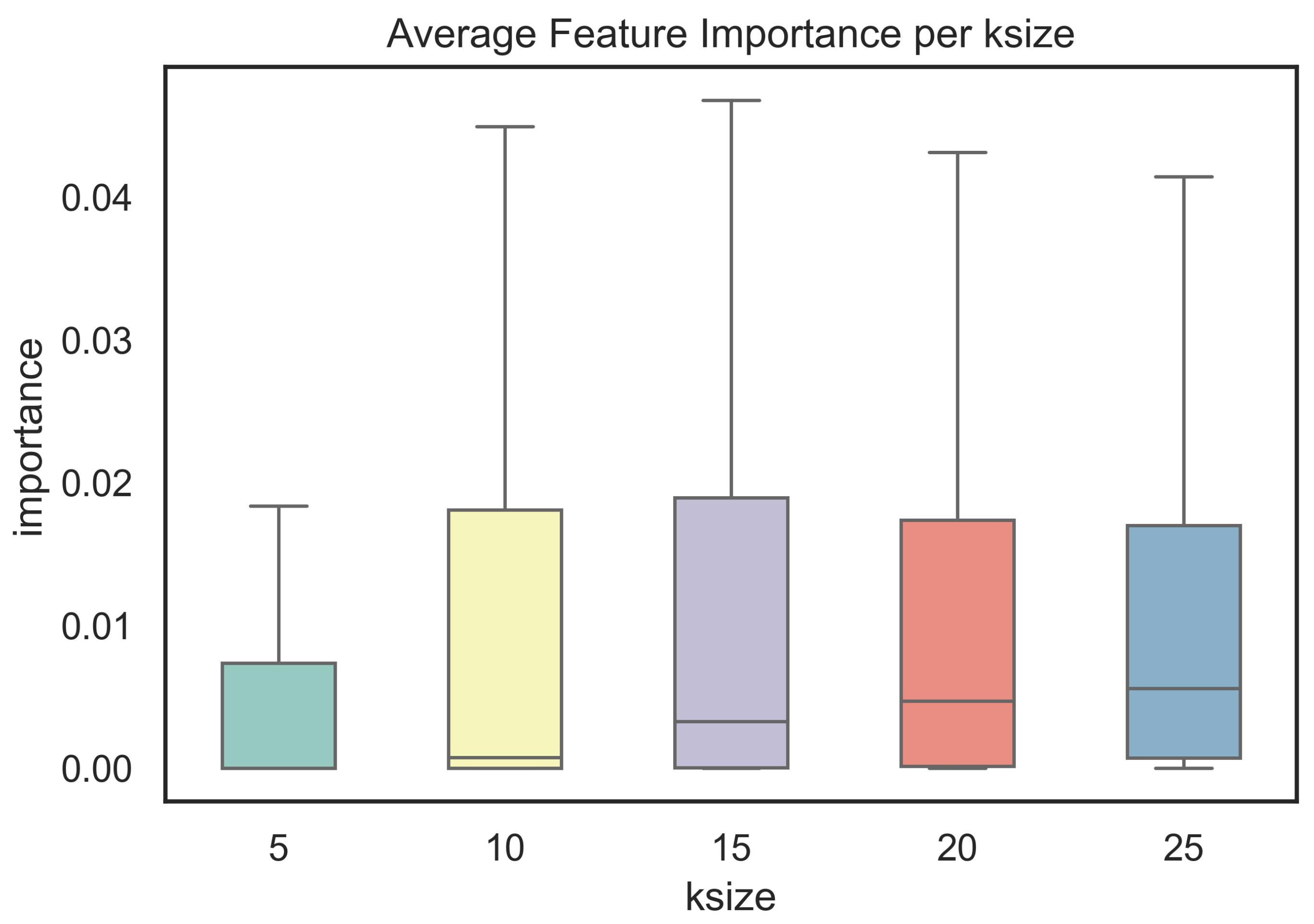
| Ksize | Count | Mean | Std | Min | 25% | 50% | 75% | Max |
|---|---|---|---|---|---|---|---|---|
| Ksize 5 | 1200 | 0.005833 | 0.013386 | 0 | 0 | 0 | 0.007345 | 0.134498 |
| Ksize 10 | 1200 | 0.011667 | 0.021662 | 0 | 1.24 × 10 | 0.000733 | 0.018082 | 0.216028 |
| Ksize 15 | 1200 | 0.012500 | 0.020859 | 0 | 0.000031 | 0.003261 | 0.018928 | 0.218144 |
| Ksize 20 | 1200 | 0.012500 | 0.019310 | 0 | 0.000136 | 0.004696 | 0.017373 | 0.017373 |
| Entry 25 | 1200 | 0.012500 | 0.017986 | 0 | 0.000715 | 0.005582 | 0.017005 | 0.185656 |
| Ksize | Count | Mean | Std | Min | 25% | 50% | 75% | Max |
|---|---|---|---|---|---|---|---|---|
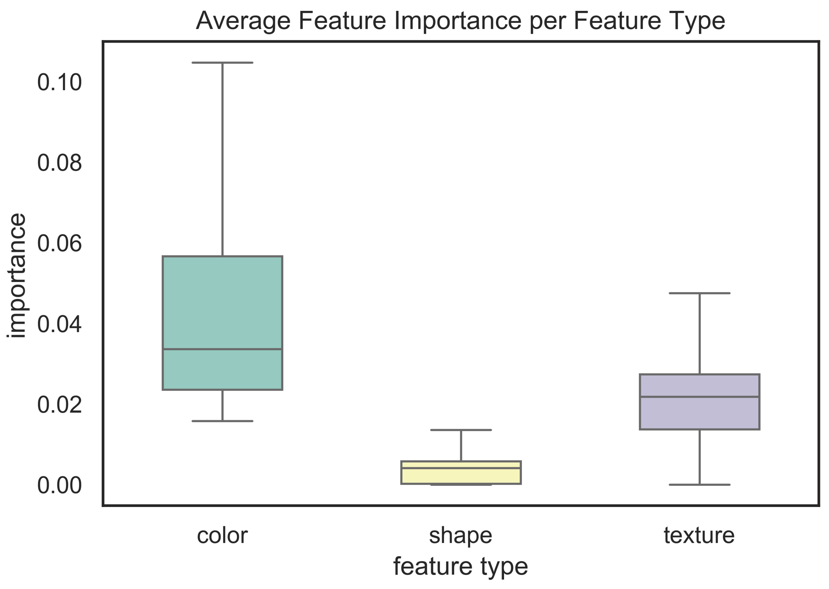
| Color | 156 | 0.043102 | 0.026751 | 0.015766 | 0.023544 | 0.033614 | 0.056612 | 0.185656 |
| Shape | 815 | 0.003625 | 0.003406 | 0 | 0.000186 | 0.004119 | 0.005780 | 0.014832 |
| Texture | 229 | 0.023240 | 0.011621 | 0 | 0.013738 | 0.021807 | 0.027370 | 0.058496 |
| Feature | Count | Mean | Std | Min | 25% | 50% | 75% | Max |
|---|---|---|---|---|---|---|---|---|
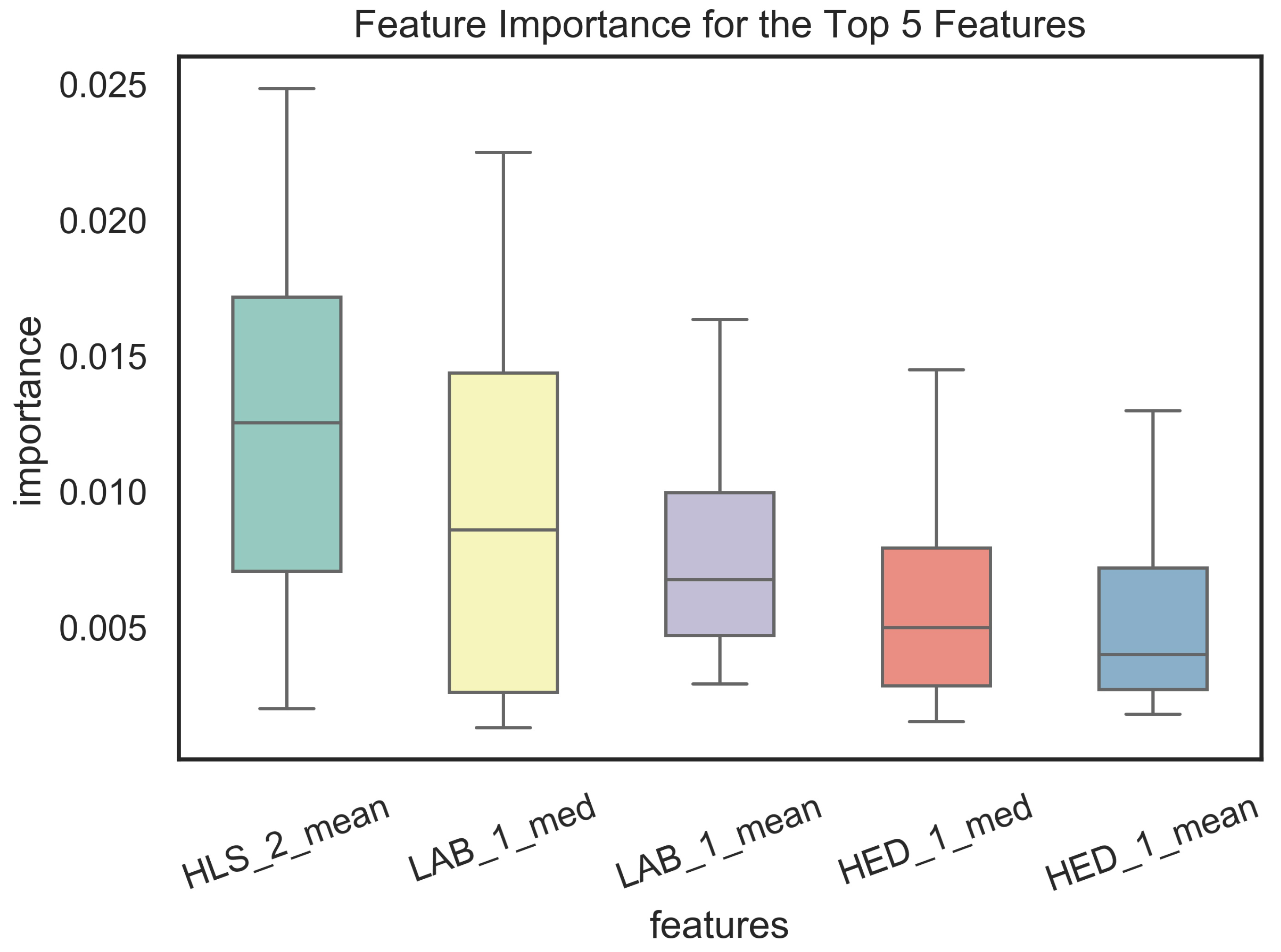
| HLS_2_mean | 15 | 0.012377 | 0.007098 | 0.002031 | 0.007076 | 0.012545 | 0.017180 | 0.024853 |
| LAB_1_med | 15 | 0.009547 | 0.007315 | 0.001328 | 0.002635 | 0.008607 | 0.014378 | 0.022514 |
| LAB_1_mean | 15 | 0.007753 | 0.004246 | 0.002942 | 0.004711 | 0.006776 | 0.009983 | 0.016350 |
| HED_1_med | 15 | 0.006981 | 0.005926 | 0.001548 | 0.002860 | 0.005006 | 0.007932 | 0.021296 |
| HED_1_mean | 15 | 0.006846 | 0.006392 | 0.001821 | 0.002721 | 0.004022 | 0.007194 | 0.023355 |
| Papers | Dataset | Use Cases | Method | Result |
|---|---|---|---|---|
| [75] | CAD files of the PCB and bare PCB image datasets | PCB inspection | LIF (Learning Inspection Features) and OLI(On-line Inspection) | Detection accuracy exceeded 97%. |
| [72] | Bounding box PCB image datasets | Detecting specific PCBs and recognizing mainboards | ORB features and Random Forest | The PCB recognition accuracy is 98.6% and the classification accuracy is 83%. |
| [73] | Bounding box PCB image datasets | Component analysis, IC detection and localization | YOLO, Faster-RCNN, Retinanet-50 | The mean average precision of these 3 techniques are: 0.698, 0.783 and 0.833. |
| [74] | Semantic PCB image datasets | PCB element detection | SSD neural network | The mean average precision of normal, enhanced, and ideal images are 0.9209, 0.9272, and 0.9510. |
| [76] | Bare PCB image datasets | Defect detection and classification | Image processing and flood fill operation | Classified up to 7 defects and the defects are identified successfully. |
| Our work | Semantic PCB image datasets | Analyzing a variety of common computer vision-based features for the task of PCB component detection | 34 feature extraction methods for color, shape, and texture; Random Forest | For most of the cases, color features demonstrated higher levels of importance in PCB component detection than shape and texture features. |
Publisher’s Note: MDPI stays neutral with regard to jurisdictional claims in published maps and institutional affiliations. |
© 2022 by the authors. Licensee MDPI, Basel, Switzerland. This article is an open access article distributed under the terms and conditions of the Creative Commons Attribution (CC BY) license (https://creativecommons.org/licenses/by/4.0/).
Share and Cite
Zhao, W.; Gurudu, S.R.; Taheri, S.; Ghosh, S.; Mallaiyan Sathiaseelan, M.A.; Asadizanjani, N. PCB Component Detection Using Computer Vision for Hardware Assurance. Big Data Cogn. Comput. 2022, 6, 39. https://doi.org/10.3390/bdcc6020039
Zhao W, Gurudu SR, Taheri S, Ghosh S, Mallaiyan Sathiaseelan MA, Asadizanjani N. PCB Component Detection Using Computer Vision for Hardware Assurance. Big Data and Cognitive Computing. 2022; 6(2):39. https://doi.org/10.3390/bdcc6020039
Chicago/Turabian StyleZhao, Wenwei, Suprith Reddy Gurudu, Shayan Taheri, Shajib Ghosh, Mukhil Azhagan Mallaiyan Sathiaseelan, and Navid Asadizanjani. 2022. "PCB Component Detection Using Computer Vision for Hardware Assurance" Big Data and Cognitive Computing 6, no. 2: 39. https://doi.org/10.3390/bdcc6020039
APA StyleZhao, W., Gurudu, S. R., Taheri, S., Ghosh, S., Mallaiyan Sathiaseelan, M. A., & Asadizanjani, N. (2022). PCB Component Detection Using Computer Vision for Hardware Assurance. Big Data and Cognitive Computing, 6(2), 39. https://doi.org/10.3390/bdcc6020039