Article

A Hierarchical Hadoop Framework to Process Geo-Distributed Big Data

by
Giuseppe Di Modica
1,† and
Orazio Tomarchio
2,*,†
1
Department of Computer Engineering, University of Bologna, Viale del Risorgimento 2, 40136 Bologna, Italy
2
Department of Electrical, Electronic and Computer Engineering, University of Catania, Viale A. Doria 6, 95125 Catania, Italy
*
Author to whom correspondence should be addressed.
These authors contributed equally to this work.
Big Data Cogn. Comput. 2022, 6(1), 5; https://doi.org/10.3390/bdcc6010005
Submission received: 8 November 2021 / Revised: 27 December 2021 / Accepted: 30 December 2021 / Published: 6 January 2022
(This article belongs to the Special Issue Big Data Analytics and Cloud Data Management)

Abstract

:
In the past twenty years, we have witnessed an unprecedented production of data worldwide that has generated a growing demand for computing resources and has stimulated the design of computing paradigms and software tools to efficiently and quickly obtain insights on such a Big Data. State-of-the-art parallel computing techniques such as the MapReduce guarantee high performance in scenarios where involved computing nodes are equally sized and clustered via broadband network links, and the data are co-located with the cluster of nodes. Unfortunately, the mentioned techniques have proven ineffective in geographically distributed scenarios, i.e., computing contexts where nodes and data are geographically distributed across multiple distant data centers. In the literature, researchers have proposed variants of the MapReduce paradigm that obtain awareness of the constraints imposed in those scenarios (such as the imbalance of nodes computing power and of interconnecting links) to enforce smart task scheduling strategies. We have designed a hierarchical computing framework in which a context-aware scheduler orchestrates computing tasks that leverage the potential of the vanilla Hadoop framework within each data center taking part in the computation. In this work, after presenting the features of the developed framework, we advocate the opportunity of fragmenting the data in a smart way so that the scheduler produces a fairer distribution of the workload among the computing tasks. To prove the concept, we implemented a software prototype of the framework and ran several experiments on a small-scale testbed. Test results are discussed in the last part of the paper.

1. Introduction

In recent years, the continuous increase in data generated and captured by organizations for very different purposes has attracted great attention from both academia and industry. The appropriate management of huge amounts of structured or unstructured data has become a key research challenge as witnessed by the explosion of research papers in this area [1,2,3]. Although much effort has been put into devising effective solutions for crunching Big Data in a single, yet powerful cluster of nodes [4], there has lately been a growing demand for processing and analyzing data that are generated and stored across geo-distributed data centers, to also meet the emerging challenges of green and sustainable computing [5].
Such a scenario calls for innovative and smarter computing frameworks capable of coping with a tough environment characterized by medium-to-big sized data volume spread across multiple heterogeneous data centers connected to each other via geographic network links. It is quite intuitive that the old strategy of aggregating such (big) distributed data into one single data center for elaboration is inefficient as well as not sustainable [6,7]. The research community addressed this problem by proposing solutions which mainly inspire to the MapReduce paradigm [8]. However, current MapReduce implementations such as the Hadoop framework [9] fail to provide effective “resource-aware” job scheduling for clusters running in geographically dispersed data centers [10], thus leading to unpredictable and often poor performance. Poor performance is due to both the heterogeneity of clusters’ computing resources and the very scarce bandwidth of the links interconnecting these clusters if compared to that of the computing environments where Hadoop has traditionally been deployed (i.e., a single cluster composed of homogeneous nodes networked by a high-speed LAN).
Solutions to this issue have been proposed by many researchers [11,12,13]. In Section 6, we propose a survey of some of the relevant literature proposals in the field. A thorough analysis of such works revealed that authors took into account only partial information of the actual geographical context. The approach we propose can be distinguished in that it leverages the whole set of the context information.
In [14], we introduced our proposal called Hierarchical Hadoop Framework (H2F). The proposal takes into account the actual heterogeneity of nodes, network links and data distribution among geographically distant sites. The proposed computing framework adopts a hierarchical approach, where a Top-level layer takes care of serving the submitted jobs and coordinates the actual computing resources that populate the Bottom-level layer. A scheduler splits a submitted job into multiple MapReduce sub-jobs which are then placed on Bottom-level resources (Sites) where target data originally reside. In [15], we conducted a study aimed at assessing the potential benefit of fragmenting the data residing in the data centers into smaller pieces and flexibly redistributing those pieces among the data centers in such a way that would benefit the computing performance of the overall MapReduce job.
Motivated by the results of the mentioned study of the impact of data fragmentation on the job performance, we decided to make the job scheduler’s strategy capable of exploiting such a powerful feature. In this paper, we propose the design and implementation of a smart data fragmentation strategy and present the results of preliminary tests. The results prove that the enhanced strategy can bring a considerable shortening of the job makespan. Further tests were also run in order to assess how powerful the proposed approach is with respect to a vanilla Hadoop framework in imbalanced geographical computing contexts.
The remainder of the paper is organized as follows: In Section 2, we briefly introduce the background of the work and depict a motivating scenario. In Section 3, we discuss the design principles of the framework. The novel data fragmentation strategy is addressed in Section 4. In Section 5, we present the results of the experiments conducted on a real test-bed. A critical review of the literature is conducted in Section 6. Final remarks and conclusion are reported in Section 7.

2. Background and Motivating Scenario

The number of applications that need to access to large volumes of distributed data is nowadays more and more increasing. Huge amount of data are generated by social network applications worldwide. Those data are usually stored on several data centers typically located in different regions. Thus, in order to obtain effective and timely results, the analysis process of these geographically dispersed data has to be thoroughly designed [16]. Multinational retailers are used to generate up to petabytes of data in one day. Data generated by the company’s points of presence are shifted to geographically distributed data centers where they are promptly processed. Again, since data are natively distributed, data processing strategies usually employed in a single-site scenario are not effective. Many IoT-based applications such as, e.g., climate monitoring and simulation handle huge volumes of data sensed from multiple geographic locations. If computing resources reside close to the sensors, as nowadays happens in many fog computing scenarios [17], the exploitation of local computing power would be a wiser choice than moving all data from the distributed locations to a central computing unit.
Big Data processing frameworks such as MapReduce [8] and Hadoop [9] have been designed to efficiently analyze large datasets stored on a single data center. Apache Hadoop, which is the main open-source platform implementing the MapReduce parallel computing paradigm, leverages the power provided by many computing nodes to increase the data analysis speed. Unfortunately, Hadoop offers high computing performance only for data stored on a single data center, realized by clusters of homogeneous computing resources, connected by high-speed network links [7].
Mining big volumes of data natively distributed over multiple and often distant places is the common need of the “geographical” scenario depicted above. In this scenario, computing resources are heterogeneous, are physically located in the considered places along with portion of the whole data and are interconnected with each other by means of network links that are far slower than those interconnecting the nodes of a cluster. None of the constraints under which Hadoop can guarantee a boost of performance applies.
The work discussed in this paper addresses the above-mentioned issues. Specifically, the focus is put on three dimensions of imbalance: (1) the non-uniform size of the data scattered throughout the computing context, (2) the inhomogeneous capability of the computing resources on which the jobs run and (3) the uneven speed of the network links interconnecting the computing resources. Such a threefold imbalance exacerbates the problem of executing an efficient computation on Big Data.
In the following section, we present a motivating scenario that guided us through the design of the proposed solution. Let us assume that Company A is running its business in multiple countries worldwide, and that in every country, a point of presence (Site, from now on) collects data from the company’s processes. Each Site runs a local data center equipped with some computing resources. Computing resources owned by a Site are interconnected by means of high-speed links (intra-Site links) to form a powerful cluster. Sites are connected to one another via a Virtual Private Network (VPN) set up over geographic network links (inter-Site links). In addition, all resources (both computing and links) are virtualized in order to form a cloud of resources that can be flexibly configured according to the need.
Suppose that each Site produces some raw data that need to be mined and that the amount of such data varies from Site to Site. Suppose also that the computing power that each Site is capable of devoting to the mining purpose is different from Site to Site. A snapshot of the just-described situation is represented in Figure 1. The company needs a way to quickly crunch all distributed data by means of some parallel computing techniques that exploit, at best, the heterogeneous resources provided by its own computing infrastructure. Basically, our proposal grounds on the idea of giving all Sites a mining task that is proportional to its computing power, i.e., the more powerful the Site the more data it has to mine. Since the distribution of the data does not follow the distribution of the computing power (a big amount of data might happen to reside in a low-power Site), the solution we propose features the shift of data from low-powered Sites (e.g., S i t e 1 ) to high-powered Sites (e.g., S i t e 4 ). Since those data movements would happen through inter-Site links, which are known to be slow, a cost is incurred in terms of time wasted. In the rest of the paper, we try to provide an answer to the problem of how to best exploit the most powerful Sites while minimizing the cost incurred for shifting data from Site to Site.
We also remark that the proposal presented in this paper is application-agnostic, i.e., it does not aim at devising a solution that fits a specific application or application pattern. Rather, in the proposed model, an application is seen as a black box capable of consuming some input data and producing some output data in a given time span, regardless of the algorithm that implements the data processing. We characterize applications by their “computing profile”, which is the application’s computing footprint calculated by just observing the black box and analyzing the data input/output balance and processing time. Based on this feature and other parameters of the distributed context environment, the framework is capable of suggesting a job schedule that optimizes any application’s performance. With that said, the framework does not prevent that further performance enhancements can be achieved by refining the application’s algorithm implementing the computation itself.

3. Hierarchical Hadoop Framework Design

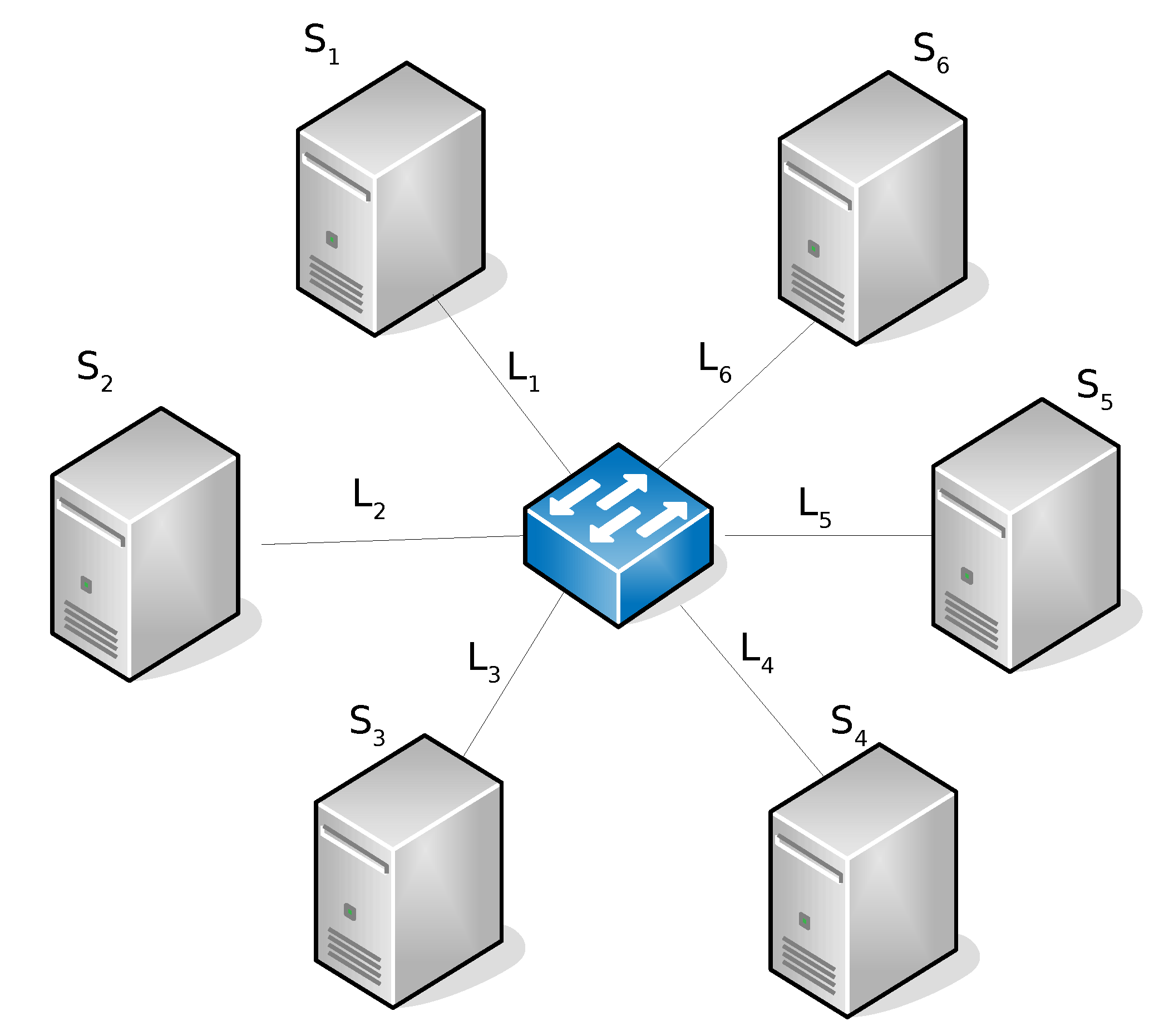
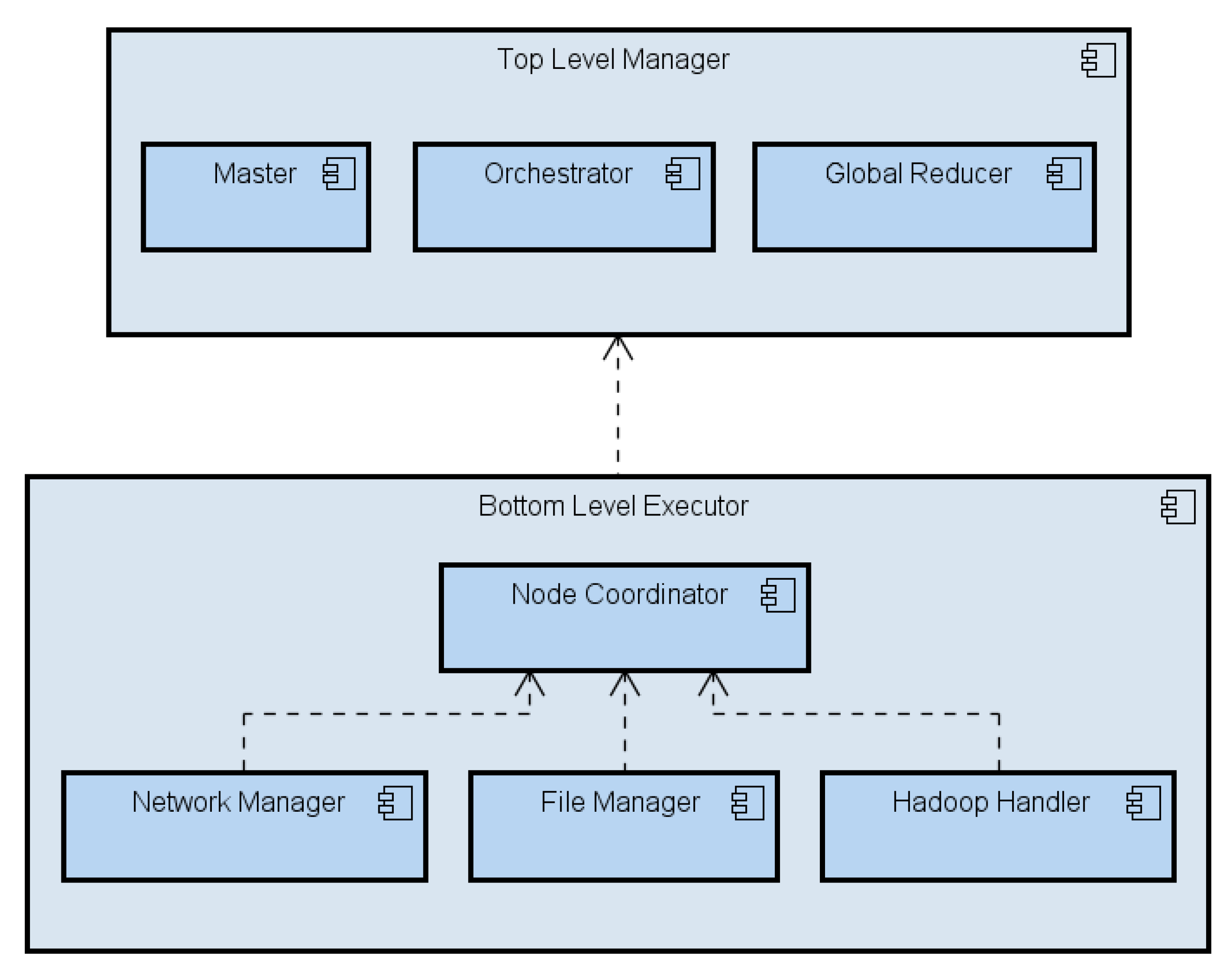
3.1. System Architecture

In the MapReduce computing paradigm, a job is a computation request that can be submitted for processing [8]. When a job is submitted, a scheduler splits it in many tasks that are mapped to available computing nodes of a cluster. A typical measure of the performance of a job processing is the makespan, i.e., the time taken for the completion of a job processing. Besides the size of the data being processed, that time is impacted by (i) the job’s execution flow devised by the scheduler (the tasks sequence) and (ii) the computing power provided by the cluster nodes hosting the tasks.
In an imbalanced computing context, things become more complicated. When a job is submitted, the question is how to best schedule imbalanced resources over unevenly distributed data in such a way that the job completion time is minimized. We address the context imbalance problem by adopting a hierarchical approach to the parallel data computation. According to this approach, a Top-level layer is responsible for running the logic to sense the computing context’s features and orchestrating smart computing plans, while a Bottom-level layer is in charge of enforcing the plans while exploiting well-known parallel computing techniques. The Top-level layer, therefore, is where smart decisions must be made in respect to, e.g., which of the many chunks of sparse data should be mined by a given computing resource. Basically, instead of letting the data be computed by resources that reside at the same data place, the intuition here is to move data wherever the largest possible computing power is available, provided that the benefit gained from the exploitation of the best computing resources overcomes the cost incurred for moving the data close to those resources. In order to support smart decisions at this level, we designed and implemented a graph-based meta-model capable of capturing the characteristics of the distributed computing contexts (in terms of computing resources, network links and data distribution) and of representing the job’s potential execution paths in a structured way (see Section 3.2.1 for details). The Bottom-level layer, instead, is where the actual computation occurs, and is populated by dummy computing resources capable of running naive parallel computing algorithms.
In summary, the H2F is based on the idea of obtaining the most powerful computing resources to (a) attract as many data chunks as possible, (b) aggregate them and (c) run plain MapReduce routines on the overall gathered data. The proposed approach does not intend to deliver a new parallel computing paradigm for imbalanced computing contexts. It rather aims at preserving and exploiting the potential of the current parallel computing techniques, even in tough computing context, by creating two management levels that cater to the needs of smart computation and the needs for fast computation, respectively.
The solution we propose is depicted in the scenario of Figure 2. Computing Sites populate the bottom level of the hierarchy. Each Site owns a certain amount of data and is capable of running plain Hadoop jobs. Upon the reception of a sub-job request from the Top-level, a Site performs the whole MapReduce execution flow on the local cluster(s) and returns the result back to the Top-level. The Top-level Manager owns the system’s business logic and is in charge of the management of the imbalanced computing context. Upon the submission of a Top-level job, the business logic schedules the set of sub-jobs to be spread throughout the distributed context, collects the sub-job results and packages the overall calculation result. In the figure, a typical execution flow, which is triggered by the submission of a Top-level job, is described by the numbered arrows. This specific case involves a shift of data from one Site to another Site (namely, from S i t e 1 to S i t e 4 ) and the run of local MapReduce sub-jobs on two Sites ( S i t e 4 and S i t e 2 ). In the considered case, S i t e 3 did not take part to the computation. Here follows a step-by-step description of all actions depicted in Figure 2 which the system had to take in order to serve the Top-level job:
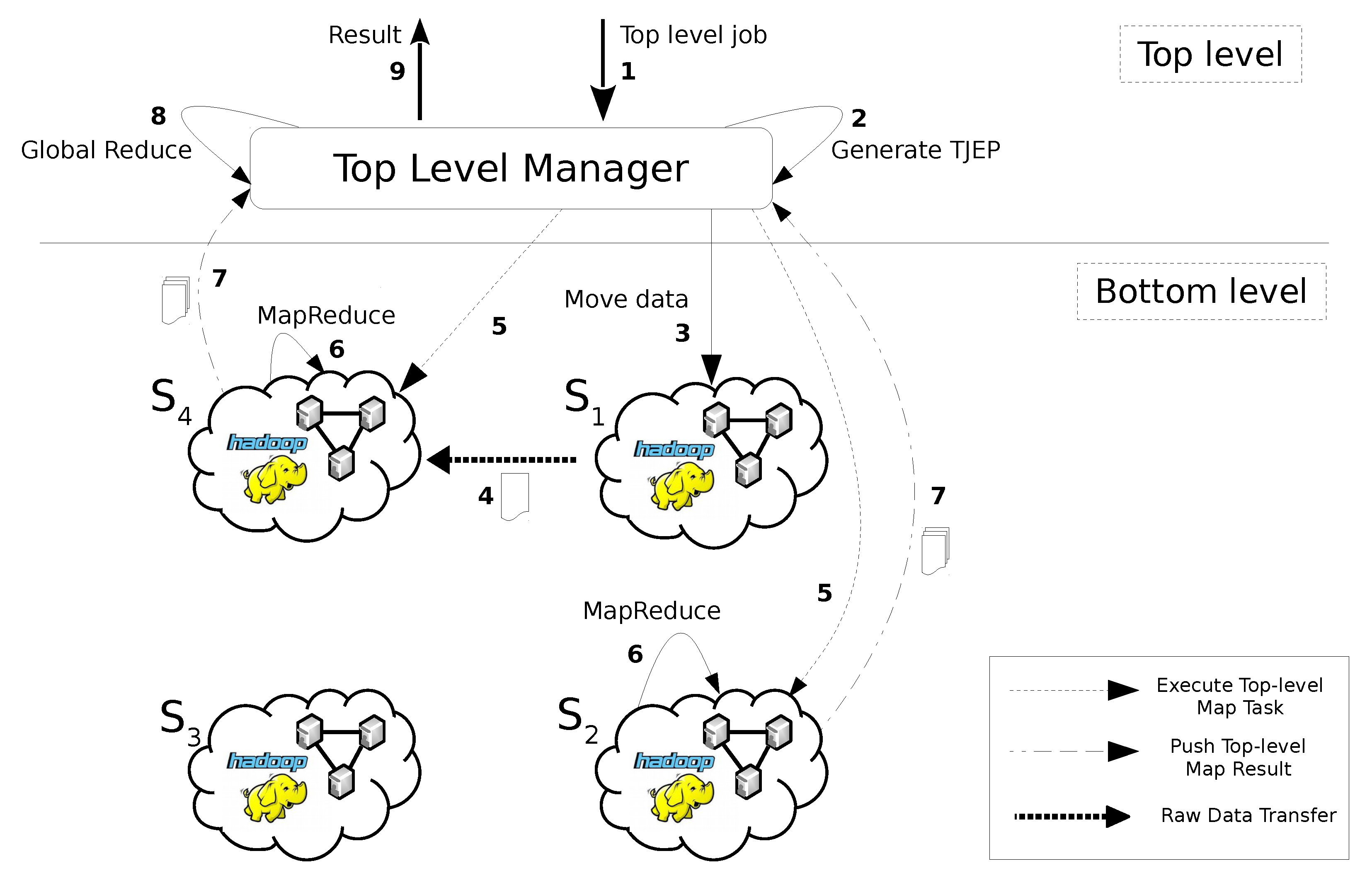
  • The Top-Level Manager receives a job submission which requires computation of data residing on S i t e 1 , S i t e 2 and S i t e 4 , respectively.
  • A Top-level Job Execution Plan (TJEP) is generated using information on (a) the status of the Bottom-level layer such as the distribution of the data set among Sites, (b) the current computing availability of Sites, (c) the topology of the network and (d) the current capacity of its links.
  • The Top-Level Manager executes the TJEP. Following the plan instructions, it orders S i t e 1 to shift its own data to S i t e 4 .
  • The actual data shift from S i t e 1 to S i t e 4 happens.
  • According to the plan, the Top-Level Manager sends a message to activate the run of sub-jobs on the Sites where the interested data are currently stored. In particular, Top-level Map tasks are triggered to run on S i t e 2 and S i t e 4 , respectively, (we reiterate that a Top-Level Map task corresponds to a MapReduce sub-job).
  • S i t e 2 and S i t e 4 executes local Hadoop sub-jobs on their respective data sets.
  • S i t e 2 and S i t e 4 send the output of their local executions to the Top-Level Manager.
  • A procedure run by the Top-Level Manager is fed with the partial results elaborated by the Bottom-Level layer and performs a global data reduction.
  • The final output is returned to the requester.
Figure 2. Job execution flow.
Bdcc 06 00005 g002
The whole process is transparent to the requester, who just has to provide the job and a pointer to the data to be processed. The design of the job execution process depicted in Figure 2 takes into consideration the imbalances of the distributed computing infrastructure in terms of computing power that the Sites are provided with, bandwidth of the inter-Site network links and data distribution. In this work, we assume that all Sites are equipped with mass-storage devices ensuring comparable I/O performance. The procedure we designed to make an estimate of the application profile [18] leverages this assumption.
The H2F logical architecture (see Figure 3) is made up of several modules that are in charge of taking care of the steps of the job’s execution flow depicted in Figure 2. In actuality, each Site is an independent system that runs an instance of the architecture in one of two distinctive modes according to the role to be played. Out of the participating Sites, only one can activate the orchestrating mode that lets the Site play the Top-Level Manager role; the Top-Level Manager owns the “smart” orchestrating business logic of the system and coordinates all the system activities. The rest of Sites have to activate the computing mode that entitles them to act as Bottom-Level Executors, i.e., those who execute the dirty work of data crunching.
The Top-Level Manager role is taken by enabling the following modules:
  • Master: it receives the Top-level job execution request, extracts the job information and passes it to the Orchestrator, which in its turn uses it to build the TJEP. The Master is in charge of enforcing the TJEP and, once the job has been processed by the Global Reducer, of delivering the final result to the requester.
  • Orchestrator: it builds the TJEP by combining information from the the submitted job and the execution context (such as, e.g., the Sites’ available computing power and inter-Site network capacity.
  • Global Reducer: it receives the output of the sub-jobs computation from the local Sites and runs the final reduction.
The Bottom-Level Executor role is activated by turning on the following modules:
  • Node Coordinator: owns all the information on the node (Site) status.
  • File Manager: it handles data blocks loading and storage of data blocks, while also keeping track of files namespace.
  • Hadoop Handler: it exposes vanilla Hadoop’s APIs. Basically, this module decouples the system from the underlying Hadoop-based computing platform. This way, the framework stays independent of the Hadoop flavor deployed in the local Site.
  • Network Manager: it handles inter-Sites communication.

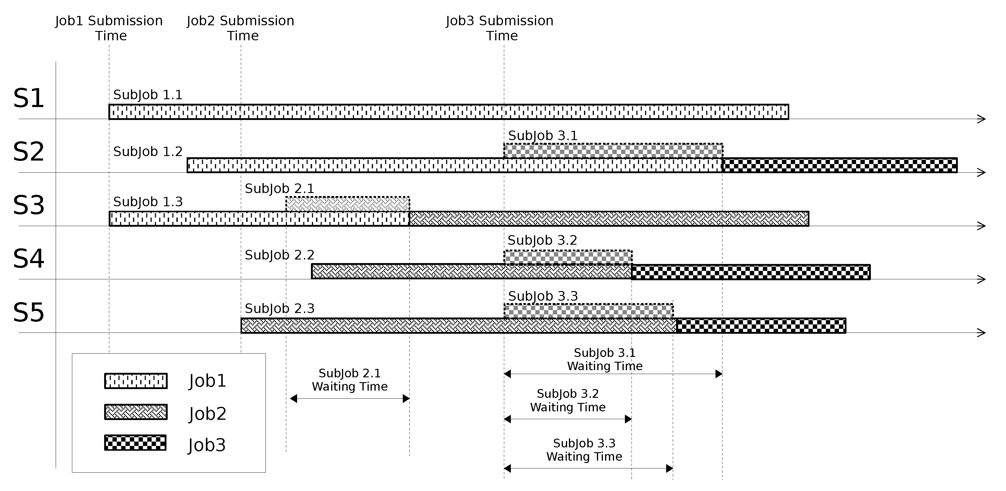
3.2. Jobs Scheduling

The TJEP built by the Orchestrator includes instructions on data redistribution among Sites as well as sub-jobs placement. To build the TJEP, the Orchestrator calls on a scheduling strategy that is capable of predicting which execution path ensures the highest job performance in terms of completion time.
Upon the submission of a new job, the job scheduler seeks for the resources that are expected to maximize the job performance. In the case that multiple jobs request the same resource at the same time, the first-come-first-served approach is enforced. While the computing resource assigned to a job is intended for the exclusive use of the job, this is not the case of network resources (Site-to-Site links), which are instead shared among the jobs that need to move data among the Sites. As a consequence, a job might have to wait for a computing resource to become available if the resource itself is momentarily accessed by another job. In addition, it might experience a further delay if its target data needs to be moved via a network link that is being shared with other jobs’ data.
In the following, we provide a simple example of how the scheduling works in the case of multiple jobs requesting the service. The reader may refer to the reference scenario represented in Figure 4.
As a distinctive feature introduced by this proposal, a job’s data can be logically and physically split into smaller data blocks of fixed size. Section 4 provides technical details on how data fragmentation is carried out. Upon a job submission, its target data can be conveniently fragmented and distributed to multiple Sites where sub-jobs eventually do the real computation.
To properly serve a job request, the scheduler must look up the resource usage plan of jobs that are being served. In the example, we show three independent jobs served according to their time of arrival. In Figure 5, we depict how the scheduler has handled the three execution requests. Based on the data fragmentation principle, each job is split into sub-jobs that run on the Sites that hold the fragmented data. For instance, J o b 1 is split into J o b 1.1 , J o b 1.2 and J o b 1.3 which run on Sites S 1 , S 2 and S 3 , respectively. In principle, a sub-job may not start its execution on a Site until data are available at that Site. This is what happens to J o b 1.2 , whose start has been delayed (notice the time gap between J o b 1 ’s submission time and J o b 1.2 ’s start time). For what concerns J o b 3 , its sub-jobs run right after J o b 3 submission, as no data shift has been decided by the TJEP. It is worth noting that while J o b 1 ’s sub-jobs may run straightaway because of availability of computing resources at the job submission time, J o b 3 ’s sub-jobs’ start is delayed until their computing resources are available ( J o b 3.1 waits until J o b 1.2 releases S 2 , J o b 3.2 waits until J o b 2.2 releases S 4 , and J o b 3.3 waits until J o b 2.3 releases S 5 ).

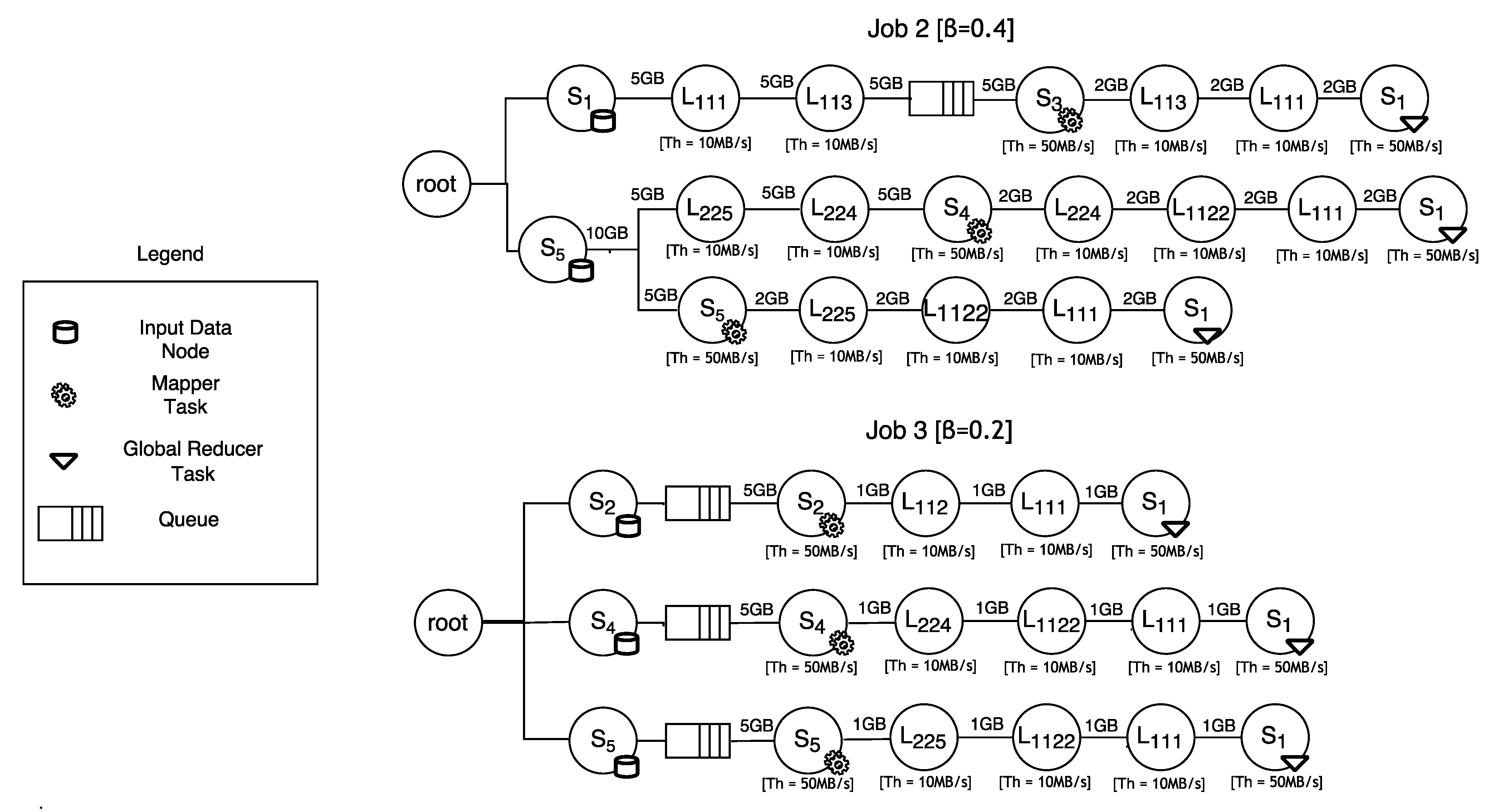
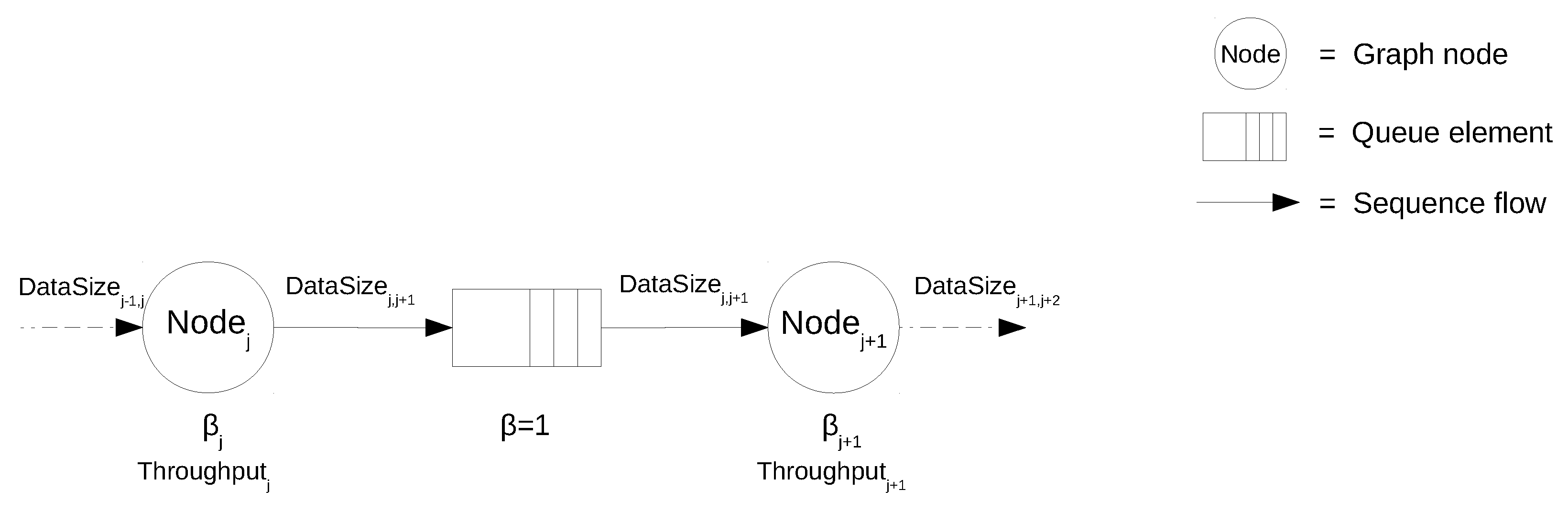
3.2.1. Modeling Job’s Execution Paths
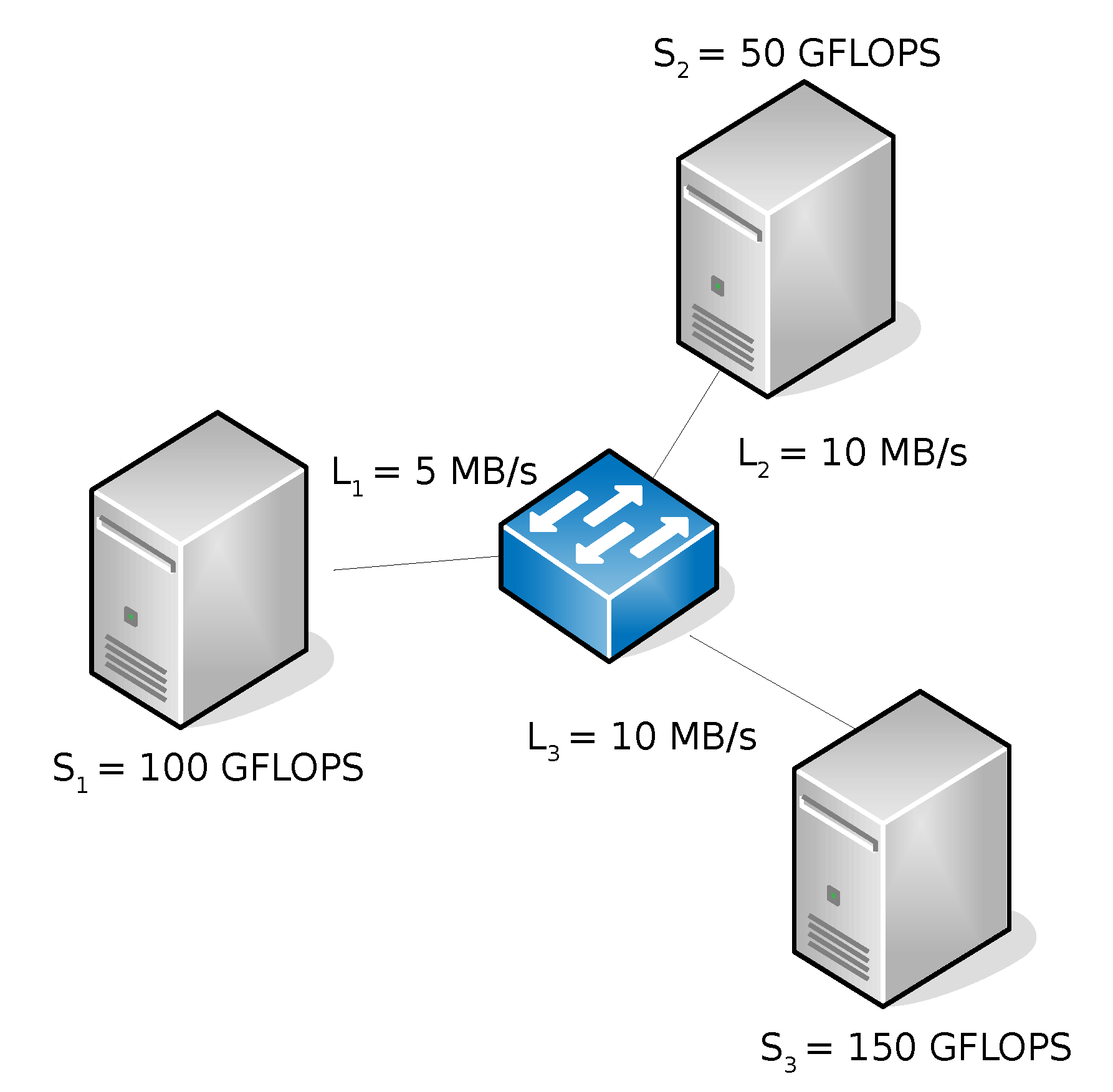
In order to guarantee a requesting job with the best execution path, three aspects must be taken into account: (1) the static features of the imbalanced computing context; (2) the overall resource occupancy at the job submission time; and (3) the features of the computation enforced by the job. We designed a graph-based representation model of a job’s execution path which accounts for the just-mentioned aspects.
By leveraging this model, the job scheduler is capable of automatically generating a finite number of potential job execution paths and then searching for the one that minimizes the job makespan. A job execution path is modeled via a sequence of actions that drive the job execution. Actions may be of three types: Site-to-Site data transfer, on-Site data elaboration and global reduction of all elaborated data. We have spoken of “potential” execution paths as there may be many alternative paths that a job may follow in its execution.
A generic job’s execution path is then represented by way of a graph whose nodes may represent a Data Computing Element (Site) or a Data Transport Element (network link) or a Queue Element. Edges between the nodes are used to model the temporal sequence of nodes in an execution path (see Figure 6). The basic idea is that each node represents an event that takes some input data, produces some output data (whose size may be different than the input’s) and consumes some time in doing that. Thus, the overall job’s execution time represented by the graph can be estimated by computing and gathering the time consumed in all the graph’s nodes. A Data Computing Element models the data elaboration by a computing element. It takes input data and outputs a data flow whose size is generally different than the input’s. The time consumed by this node depends on (a) the computing capacity of the Site it represents, (b) the job’s computation type and (c) the amount of data to be processed. A Data Transport Element models a data shift over a network link; therefore, the output data and the input data do not differ in size; the time consumed by this node is proportional to the link’s bandwidth capacity. Queue Element nodes model the delay suffered by a sub-job when it waits for an available computing resource. Queue elements do not alter the size of traversing data.
A node has two attributes: the compression factor β a p p , used to measure the data shrink/expansion introduced by a node, and the T h r o u g h p u t , defined as the amount of data per time unit that the node is capable of processing. The β a p p value for the Data Computing Element is equal to the ratio of the output data to the input data, while for the Data Transport Elements, it equals 1, as there is no modification of the data size occurring in a data transfer. The T h r o u g h p u t of a Data Computing Element depends on the Site’s computing capacity and the job’s computation type, while for the Data Transport Elements, the Throughput corresponds to the link capacity. Finally, for a Queue Element, the β a p p is set to 1 (no computation occurs); in addition, since the concept of T h r o u g h p u t is not easily applicable to this node (it would depend on the computing process of other nodes), we stick to the calculus of the delay introduced by the queue by estimating the residual computing time of the “competing” nodes (i.e., nodes of other jobs modeling the same contended computing resource).
In general, a node’s execution time is defined as the ratio of the input data size to the T h r o u g h p u t of the node. In Figure 6, the label value of the edge connecting node N o d e j to node N o d e j + 1 is given by:
D a t a S i z e j , j + 1 = D a t a S i z e j 1 , j × β j
A generic node N o d e j ’s execution time is defined as:
T j = D a t a S i z e j 1 , j T h r o u g h p u t j
Both the β a p p and the T h r o u g h p u t are job’s application specific, i.e., they depend on the particular job’s algorithm that elaborates the data. Since such values are not available at job submission time, we need to estimate them. Specifically, before the TJEC is actually elaborated by the job scheduler, we run the job’s algorithm on small-sized samples of the overall data that are actually elaborated by the job. The result of the estimate constitutes what we call the job’s Application Profile. Details on the elaboration of the Application Profile can be found in our previous work [18], where we studied the Application Profile of a well-known MapReduce applications.
As mentioned before, the execution path model is strongly affected by the computing context. The number of potential paths generated for a given job strictly depends on: (a) the capacity of available computing nodes, (b) the network links’ number and capacity and (c) the data fragmentation scheme. We provide for a split of the data set into equally sized data blocks, thus favoring the shift of certain data blocks from Site to Site. In Section 4, we report a study on the estimate of the optimum data block size. On the one hand, data granularity provides the advantage of producing more flexible data distribution schemes. As a counter effect, a large number of the data blocks gives birth to a large number of potential execution paths. Basically, a graph has as many branches as the number of Map Reduce sub-jobs that are executed. Every branch stems from the root node (initial node) and ends up at the Global Reducer’s node. A branch’s execution time is the sum of the execution times of the nodes composing the branch (with the exception of the Global Reducer node, which is left out of this summation). We outline that executions carried out along branches are independent of each other; therefore, the branches end up showing different execution times. The Global Reducer activates only when all branches have output their results. Therefore, the slowest branch determines when the global reducing is allowed to start. Finally, the Global Reducer execution time is calculated by the summing up the sizes of output received by the branches and dividing it by the node’s estimated Throughput.
Let us make a concrete example of an execution path modeling. The scenario we consider is the one depicted in Figure 4, while we also refer to the submission timing shown in Figure 5. Furthermore, we assume that data have been ideally fragmented in data blocks of 5 GB each, and that every job needs to process 15 GB of data. J o b 1 is requesting to process data that resides in S 1 (a 5 GB data block) and S 3 (a 10 GB data block, ideally splits into two 5 GB data blocks); J o b 2 is requesting to process data residing in S 1 (one data block) and S 5 (two data blocks); J o b 3 is requesting to process data residing in S 2 , S 4 and S 5 , each holding one 5 GB data block. In Figure 7, we depicted the graph model representing two potential execution paths generated by the job scheduler for J o b 2 and J o b 3 , respectively. For the clarity of the picture, we did not depict the J o b 1 . execution path. The plan for J o b 2 envisions three execution branches:
  • a data block is moved from S 1 to S 3 through the links L 111 and L 113 ; here, sub-job J o b 2.1 suffers a delay because the resource S 3 is used by sub-job J o b 1.3 (see Figure 5); once S 3 has been released, J o b 2.1 gains it and elaborates the data block; the output of the elaboration is shifted to S 1 through the links L 113 and L 111 ; here, the global reduction can take place (note that the global reduction step starts only after all the data elaborated by the sub-jobs have been gathered in S 1 .).
  • a data block is shifted from S 5 to S 4 traversing the links L 225 and L 224 ; here, J o b 2.2 immediately gains the computing resource ( S 4 ) and elaborates the data block; the output of the elaboration is moved to S 1 through the links L 224 , L 1122 and L 111 ; here, the global reduction can take place.
  • J o b 2.3 accesses and elaborates the data block residing in S 5 ; the output of the elaboration is shifted to S 1 through the links L 225 , L 1122 and L 111 ; here, the global reduction can take place.
Figure 7. Graph modeling potential execution paths for Job 2 and Job 3.
Bdcc 06 00005 g007
Likewise, the J 3 plan envisions three branches. In this case, in no branch, a data shift is necessary. It is worth noting that all sub-jobs suffers a delay, since the requested computing resources are locked by other running sub-jobs. We remark that the depicted paths are just potential execution paths devised for J 2 and J 3 . The job scheduler is charged with exploring all the potential paths of a job and identifying the one providing for the shortest execution time. For a deeper insight on the search for the optimal execution path, the reader may refer to [19], where details about the adopted LAHC algorithm can be found.

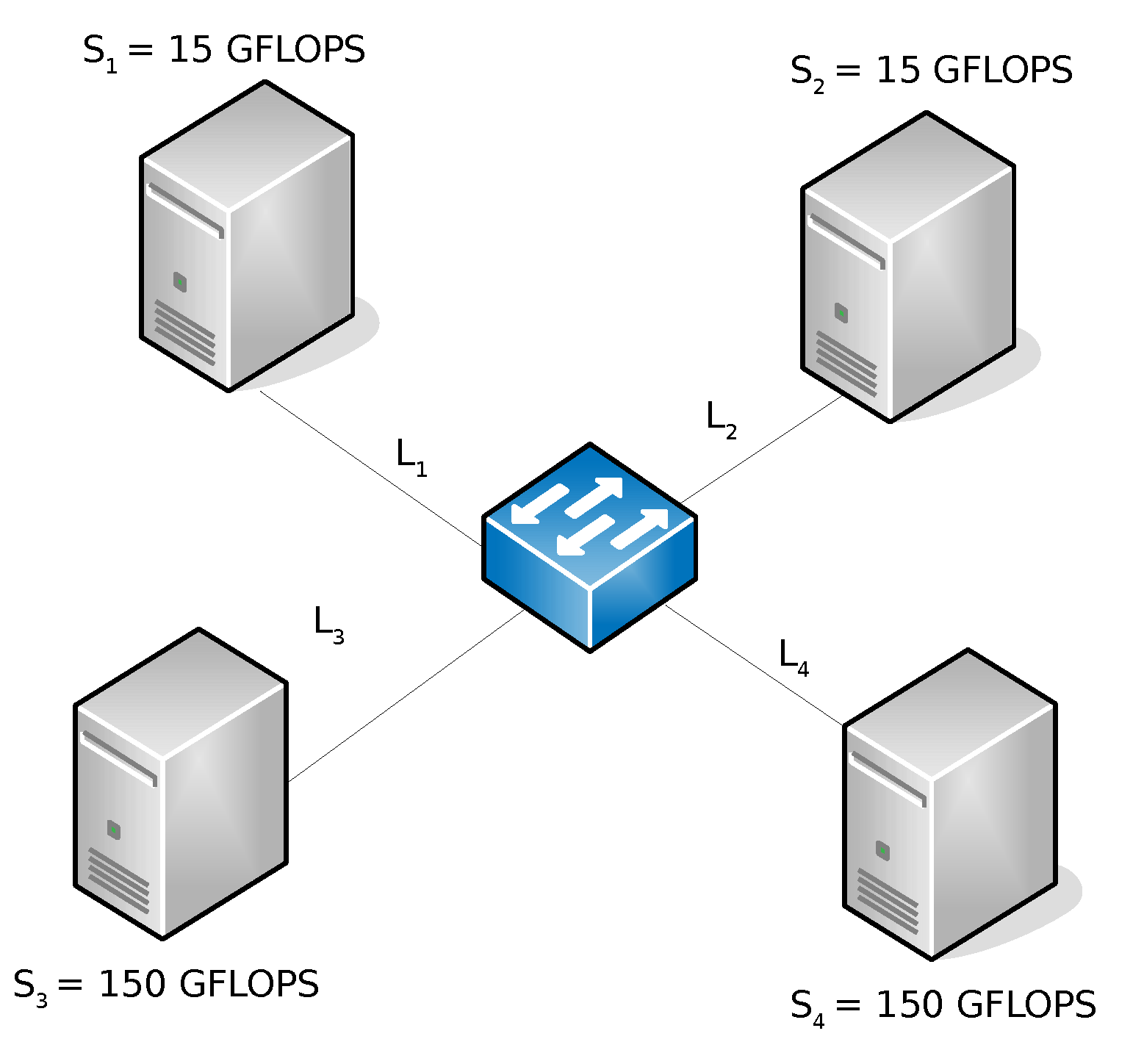
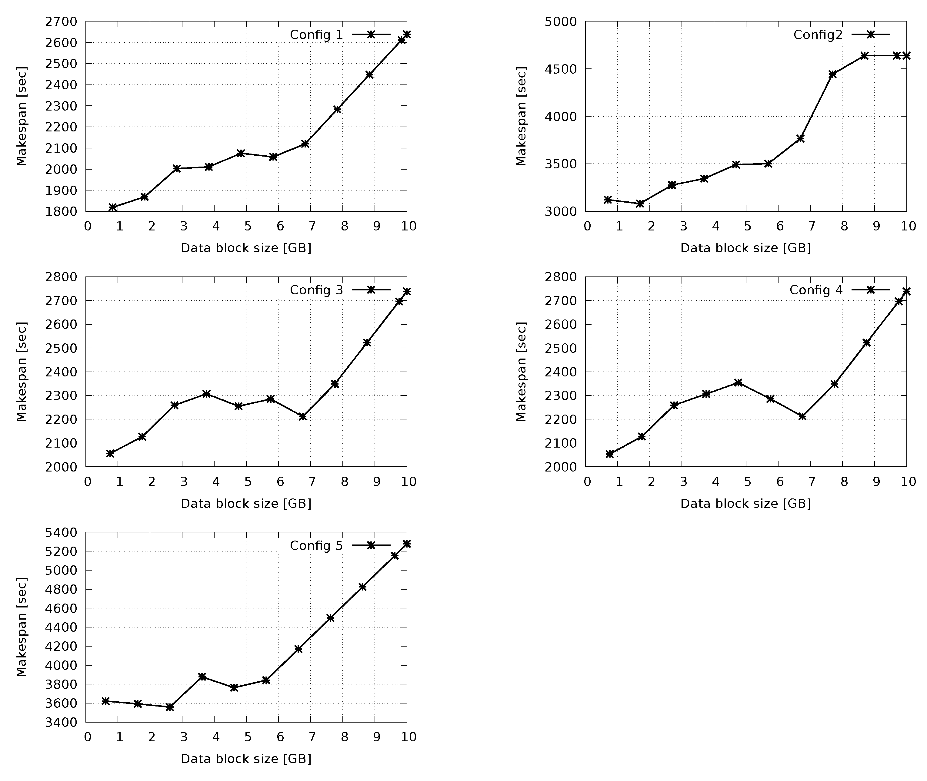
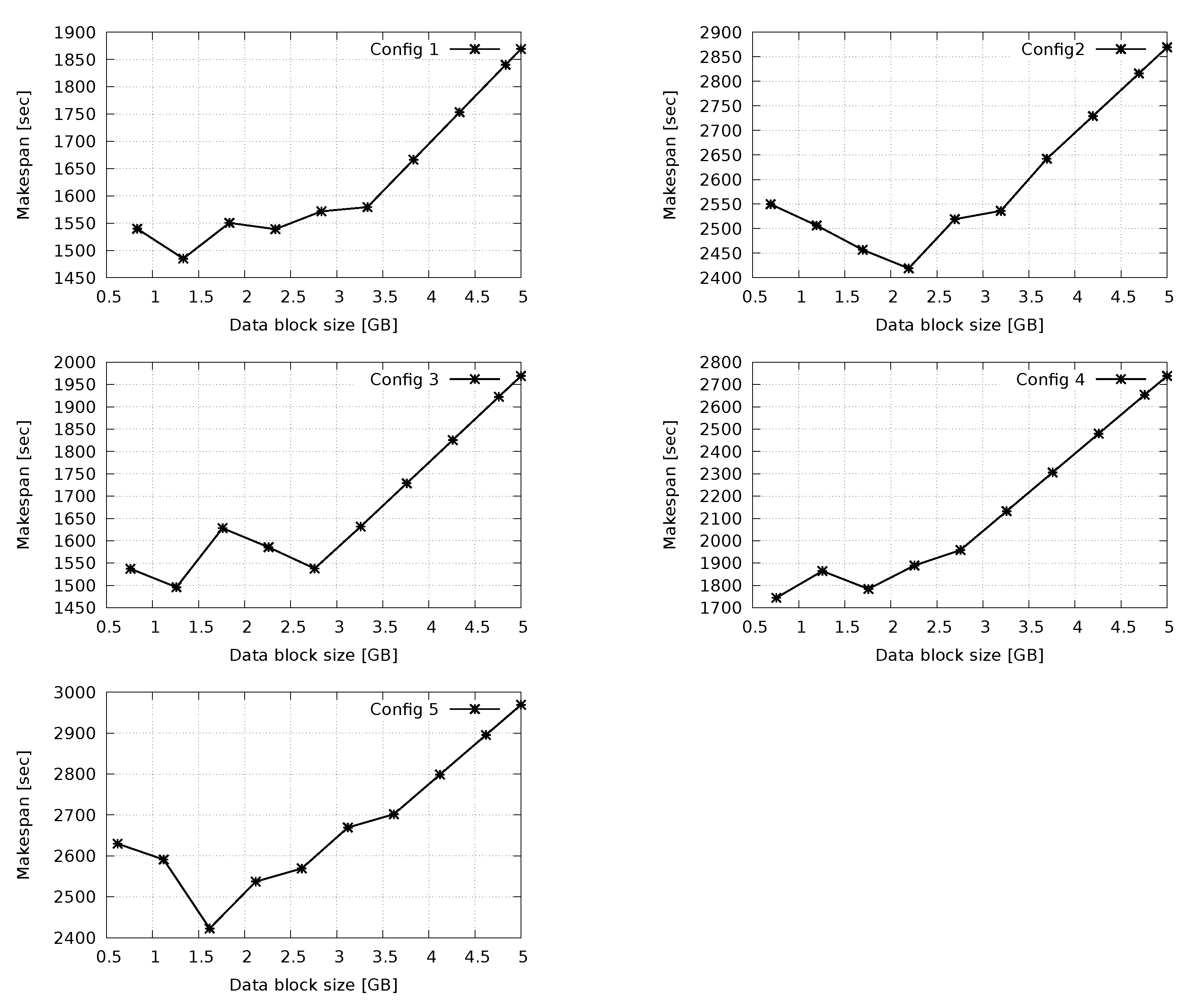
4. Optimal Data Fragmentation

As mentioned in Section 3.2.1, our approach provides for the split of the entire data set into multiple, equally sized data blocks, with the objective of shifting data blocks among Sites. In this section we study the impact of data block size on the performance of the job and propose a mechanism to estimate the data block size that maximizes that performance. Of course, the data block size is not an independent variable, and its impact must be regarded along with that of other variables that characterize the distributed computing environment, namely the available computing resources and the network links’ capacity.
We recall the intuition on which we grounded our proposal: in the aim of exploiting at best the distributed computing resources, a Site holding great computing capacity ought to attract as much data as possible, provided that the network paths traversed by those data do not penalize too much the gathering of the data at that Site. Moving data to a Site turns out to be convenient if (a) the Site offers much computing capacity and (b) the network connecting the data’s initial location and the Site’s location has a large bandwidth. To measure the fitness of a Site in regard to this purpose, we introduce the following parameters:
  • C P U r a t e is the Site’s computing power normalized to the overall context’s computing power.
  • C o n n e c t i v i t y represents the capability of the Site to exchange data with other sites in the computing context.
The C P U r a t e of Site S i is given by:
C P U r a t e ( S i ) = C P U ( S i ) j = 1 N C P U ( S j )
The C o n n e c t i v i t y of Site S i is defined as the arithmetic mean of all end-to-end nominal network bandwidths between the considered Site and the other Sites in the distributed computing context. It is represented as:
C o n n e c t i v i t y ( S i ) = j = 1 N B a n d w i d t h i , j N 1
where B a n d w i d t h i , j is the nominal network capacity between node i and node j, and N is the number of Sites belonging to the distributed context. We also define the C o n n e c t i v i t y r a t e as the connectivity of a Site normalized to the overall connectivity of the distributed context. Thus, for Site S i , it is given by:
C o n n e c t i v i t y r a t e ( S i ) = C o n n e c t i v i t y ( S i ) j = 1 N C o n n e c t i v i t y ( S j )
Now, for each Site, we compute a score as a linear function of both the C o n n e c t i v i t y r a t e and the C P U r a t e described above. The score function is given by:
S c o r e ( S i ) = K × C P U r a t e ( S i ) + ( 1 K ) × C o n n e c t i v i t y r a t e ( S i )
where k is an arbitrary constant in the range [0, 1]. We ran several tests in order to best tune the K value. In our scenarios, good results were observed by setting k values close to 0.5, i.e., values that balance the contribution of the network and of the computing power. Seeking for an optimum k value, though, was out of the scope of this work.
Finally, we define the N o m i n a l B l o c k S i z e as:
N o m i n a l B l o c k S i z e = min i S c o r e ( S i ) × J o b I n p u t S i z e
where J o b I n p u t S i z e is the total amount of data to be processed by the given Job. The N o m i n a l B l o c k S i z e is the data block size found by the described heuristic method. Of course, there is no guarantee that such a value is the optimum (i.e., the one that maximizes the job performance), but it is very likely that the optimum value is near the N o m i n a l B l o c k S i z e . A procedure is then run to seek the optimum in the proximity of the N o m i n a l B l o c k S i z e .
Given the N o m i n a l B l o c k S i z e , we generate a set of values in the range:
[ 0.5 × N o m i n a l B l o c k S i z e , M i n C h u n k S i z e ]
where M i n C h u n k S i z e is the minimum size of the data chunks located at the Sites. Regarding the setting of the lower bound of the mentioned range, we believe 0.5 · N o m i n a l B l o c k S i z e is a good compromise to start from when seeking for optimal values that are close to the N o m i n a l B l o c k S i z e and, at the same time, do not produce an excessive data fragmentation, which in turn would eventually be detrimental to the overall performance. For each data block size in the range, we compute the best job execution path by feeding the LAHC scheduling algorithm with the current context, the job information and the selected data block size [19]. Finally, the data block size producing the minimum job makespan is selected as the best candidate.
For a better comprehension of the mechanism, we provide the following example. Let us suppose that the computing context is made up of three Sites ( S 1 , S 2 and S 3 ) interconnected through a star network topology, as depicted in Figure 8. In this example, the overall data to process are 10 GB and initially reside on the following sites: S 1 1   GB , S 2 3   GB and S 2 6   GB .
The C P U r a t e , C o n n e c t i v i t y and C o n n e c t i v i t y r a t e for Site S 1 are, respectively:
C P U r a t e ( S 1 ) = 100 50 + 100 + 150 = 0.33
C o n n e c t i v i t y ( S 1 ) = 5 + 5 2 = 5
C o n n e c t i v i t y r a t e ( S 1 ) = 5 5 + 7.5 + 7.5 = 0.25
By setting K to 0.5, the score of Site S 1 is:
S c o r e ( S 1 ) = 0.5 × C P U r a t e ( S 1 ) + 0.5 × C o n n e c t i v i t y r a t e ( S 1 ) = 0.33
Similarly, the S c o r e ( S 2 ) and S c o r e ( S 3 ) are, respectively, 0.271 and 0.43. The minimum score is then on Site S 2 ; according to our approach, the selected N o m i n a l B l o c k S i z e is:
N o m i n a l B l o c k S i z e = S c o r e ( S 2 ) × J o b I n p u t S i z e = 0.271 × 10   GB = 271   MB
In this case, the optimal size search procedure has to seek for the optimal size in the range [135 MB, 1 GB], as 1 GB is the size of the smallest among the data chunks (located at S 1 ).
In order to assess the effectiveness of the discussed exploratory approach, some experiments were run. Starting from the reference scenario depicted in Figure 9, we designed some configurations (that are meant to represent different, concrete computing scenarios) by tuning up the following parameters: the CPU Power of each Site, the network links’ capacity and the initial distribution of the data among the Sites. The experiments were performed by simulating the execution of a job that needed to process 10 GB of data. Specifically, we considered a sample job for which a β a p p value of 0.5 was estimated. The parameter that is put under observation is of course the job makespan. The objective of the experiment is to prove the capability of the job scheduler to derive the execution path ensuring the job’s optimum makespan by varying the data block size. Of course, this has to hold true independently of the distributed computing scenario that is being considered.
We created five configurations, which have been reported in Table 1. Each configuration represents a specific distributed computing context. As the reader may notice, going from C o n f i g 1 to C o n f i g 5 , the computing scenarios become more and more unbalanced.
In the tests, for each configuration, the job scheduler was fed with the context data. According to our mechanism, the optimal data block size is to be sought in the range [ 0.5 × N o m i n a l B l o c k S i z e , M i n C h u n k S i z e ] . For the chosen configurations, the calculus in Formula (3) gave the values reported in Table 2.
The exploration procedure extracts a finite number of points belonging to that range and that constitute the points to be checked. The points are selected in this way: starting from the left edge of the range, the next points to be selected are obtained by stepping to the right by a fixed quantity of 10 % of the M i n C h u n k S i z e . Of course, for a finer search, a smaller step might be chosen: this would generate a higher number of points, which in turn would mean a heavier burden to the job scheduler with no guarantee of a consistent benefit.
In the first battery of tests, the job’s input data were equally spread so that Sites would host 1.7 GB data each. Results from tests run on the five configurations are shown in Figure 10, where the assessed job’s makespan is plotted against the data block size. It is important to notice that, with the exception of C o n f i g 1 , for all of the configurations the graph mainly has a parabolic trend with a clearly identified minimum, which is very close to the N o m i n a l B l o c k S i z e .
In the second battery of tests, the configurations almost remained the same; the only modification regarded the initial data placement. In particular, a single Site was chosen to host the entire 10 GB of data. For the sake of completeness, we repeated the test selecting every time a different Site to host the data. It was observed that the data’s initial placement is not a bias to the experiment. In Figure 11, we report the results of the case where the Site chosen to host the data is S 4 . This time, the trend is more like a slope, but again the minimum is localized around the N o m i n a l B l o c k S i z e .
In the last battery of tests, we split up the job’s input data into two equally sized data chunks and distributed them among two Sites in the cluster. We repeated the experiment by taking into account each pair of Sites in the scenario. The choice of the Sites pair was observed to be irrelevant. In Figure 12, the results obtained by equally distributing data on S 1 and S 3 are reported for each of the five configurations. The same consideration made before on the minimum holds here.
To conclude, the intuition that the optimal data block size depends on the connectivity and on the computing power distribution of the computing context (formalized in Formula (3)) was proved true. According to this, the procedure of the search for the optimal data block size has been embedded as a subroutine of the job scheduler to support the search for the optimal job execution path. Since the optimum data block size was always found to be close to the N o m i n a l B l o c k S i z e value, the exploration procedure focuses on a very limited boundary of that value (3–4 points are checked at most).

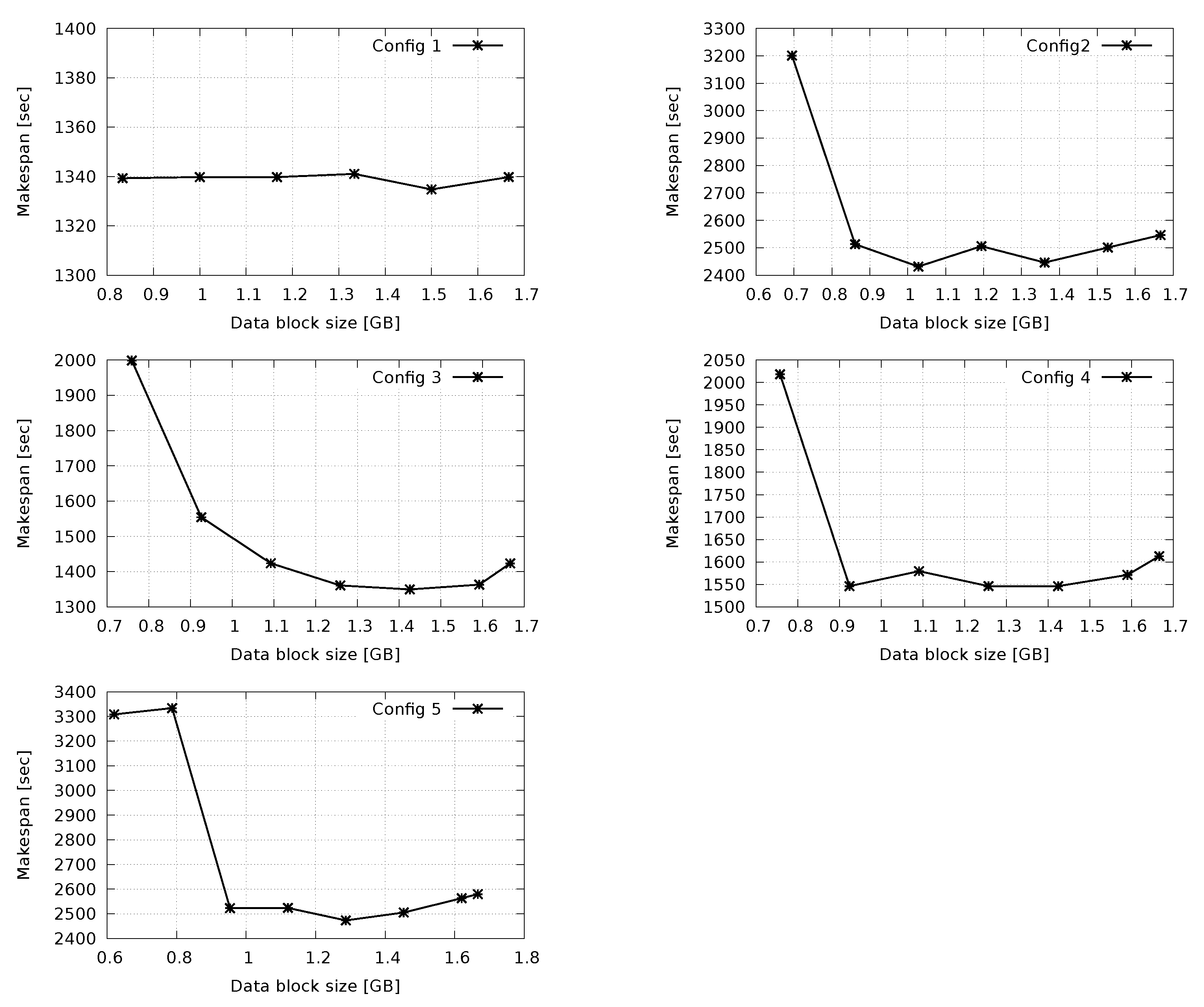
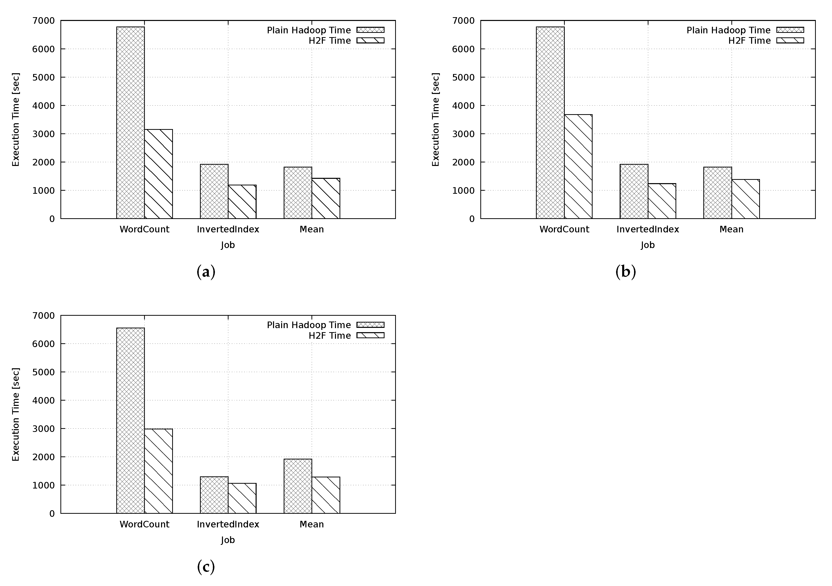
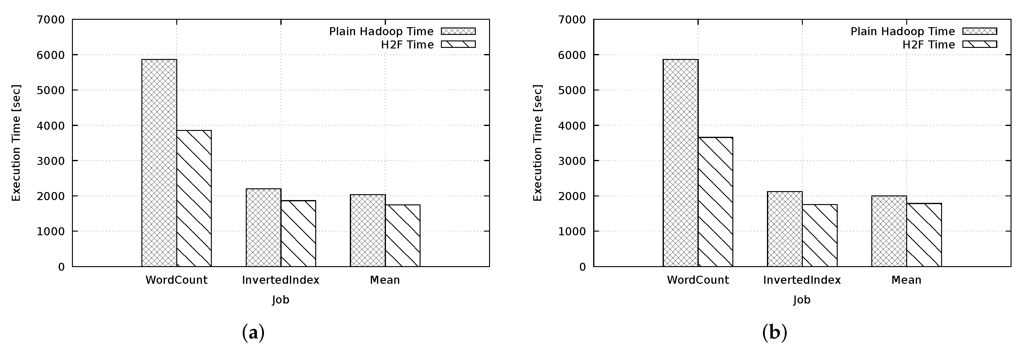
5. Experiment: H2F vs. Hadoop

In this section, we describe several tests run to estimate how well H2F performs with respect to a vanilla Hadoop framework. The job’s completion time (makespan) is KPI we used to make such comparison.
The proof-of-concept was achieved by way of a small-scale test-bed, realized by means of off-the-shelf PCs and network elements, which reproduces an imbalanced distributed computing context. The reader can notice that the size of the data involved in the experiment is also scaled to fit the test-bed dimension. The employed test-bed is a controlled environment which gave us the freedom to access and play with all infrastructural parameters of interest, from the CPU power of a Site to the bandwidth of an inter-Site link. In our future plans, we will work at the implementation of a large-scale test-bed addressing a real geographical computing scenario.
The test-bed environment consists of four Sites connected through network links. Each Site represents a data center, which is equipped with some computing power, stores some raw data and executes an instance of the H2F framework. The network topology of the test-bed environment is depicted in Figure 13. The configuration of the testbed was set as follows: two sites ( S 3 , S 4 ) equipped with an i7 CPU architecture and 8 GB RAM, which provide for an estimated computing node’s capacity of 150 GFLOPS (The computing capacity was assessed with the Linpack benchmark (http://www.netlib.org/benchmark/hpl/, accessed on 29 December 2021); two Sites ( S 1 , S 2 ) having a Core 2 Duo CPU and 4GB RAM, for an estimated computing power of 15 GFLOPS each. Therefore, in terms of computing power, the test-bed is natively imbalanced. Finally, each network link’s nominal bandwidth is set to 40 MB/s.
In order to discover how the proposed framework is capable of boosting the performance of various kind of Hadoop application, we tested three applications showing very different application profiles.
In particular, the following applications were used for the mentioned purpose: WordCount, InvertedIndex and ArithmeticMean. Those applications represent a (yet non-exhaustive) set of applications that can be easily MapReduced. WordCount is the most I/O bound and is very CPU intensive too, while ArithmeticMean is CPU intensive and does not interact much with I/O. In its turn, InvertedIndex is as CPU intensive as the other applications but stays in the middle for what concerns interaction I/O. The reader may refer to our former work [18] for a detailed characterization of these applications in terms of β a p p and T h r o u g h p u t .
Some testing scenarios, reproducing different situations of imbalance, were specifically designed to analyze the capability of H2F in boosting the performance of Hadoop in distributed computing contexts where imbalance exists in terms of Sites’ computing capacity, network links’ bandwidth and raw data distribution, respectively. The scenarios were generated by tuning up the initial distribution of the raw data among the sites and the capacity of the network links interconnecting the sites.
The first scenario focuses on data distribution. The size of raw data considered in this scenario is 5 GB. The configurations used for this test are reported in Table 3. For each configuration, the displayed values represent the rate of the overall input data residing in each Site. For instance, in C o n f i g 1 , 40% of the data resides in S 1 , 30% in S 2 , 20% in S 3 and 10% in S 4 .
Results of the tests run to compare the performance of H2F and the Hadoop on the three applications are reported in Figure 14.
The depicted results are averaged through 10 runs per configuration. All values include the overhead time, which is the time spent to prepare the data for the processing. In the case of the H2F, the overhead is composed of: the time for the Job scheduler to devise the optimal execution path and the optimal data block size; (optionally) the time to shift data among Sites; the time taken by the selected Site to store the received data in the local HDFS; the waiting of the Global Reducer. In the case of vanilla Hadoop, the overhead is just the time to store the data in the HDFS. In regards to the H2F, the job scheduling time never exceeded a hundred seconds. Of course, that time may increase in the case of more complex network topologies and larger amounts of raw data.
Taking a look at Figure 14, we may notice that, regardless of the initial distribution of data, the H2F framework executes the WordCount application quicker than Hadoop. As for the other two applications, the performances are comparable in the case of C o n f i g 1 and C o n f i g 2 , with a little advantage for H2F. In C o n f i g 3 , vanilla Hadoop slightly prevails. Let us make a few considerations on the obtained results. First, the use of the H2F in this specific scenario for applications having a profile that is similar to that of InvertedIndex and ArithmeticMean seems to not be effective; indeed, it might actually lead to a performance degradation. The bad performance of the H2F is due to the relatively small amount of data (5 GB), because of which the overhead time heavily impacts the H2F performance (at least, in a heavier way than in the case of the vanilla Hadoop framework). Second, in the case of Wordcount, the CPU-intensive nature of the application makes the H2F outperform the vanilla Hadoop, despite the former suffering from a longer overhead time. This proves that for more CPU intensive application, the H2F can deliver a better performance.
In the second scenario, we considered an overall data size of 50 GB, while keeping unchanged the rest of configurations. Results of the tests are depicted in Figure 15. With the increase in data size, H2F exhibits a better performance for all applications. The performance improvement over the vanilla Hadoop is more evident than the 5 GB case (15–20% on average). On a larger data set, the H2F is capable of detecting the computation resources that likely speed up the computing process (as they exhibit a larger computing capacity). In addition, with the job makespan being longer than in the 5 GB case, we observed a proportionally much lower impact of the overhead.
We designed one last scenario where the network links’ capacity is imbalanced with the purpose of showing that the H2F can also adapt to such an imbalance. In Table 4, we report two links’ bandwidth configurations used in the tests. The remaining parameters are left unchanged (50 GB data, input data distributed among Sites as defined in C o n f i g 1 ).
In Figure 16, we reported the results of the tests for the imbalanced links scenario. Once again, the makespan observed for the H2F is shorter than the vanilla Hadoop’s, proving that the H2F framework can also deal very well with imbalanced network configurations.

Concluding Remarks on Performance Results

The aim of all the tests was to assess the capability of the H2F to adapt to different distributed computing environments, and to also show under what conditions it may provide better performance than the vanilla Hadoop framework.
The first achieved result concerns the application profile: we found out that H2F provides better performance for CPU intensive and I/O bound applications, which in our tests are represented by the WordCount application). This holds true for different schemes of data distribution among Sites and network links bandwidth.
The second result relates to the overhead introduced by the H2F framework: for relatively small amounts of data (5 GB, in our small-scale testbed), the overhead of H2F strategy may negatively impact performance results with respect to a vanilla Hadoop framework. However this occurs only on a specific kind of application profiles, and, in general, it is not a big issue since H2F is purposefully designed to work with and in Big Data environments.
The final consideration concerns network imbalance: though it has been tested in a small testbed, the H2F has proven capable to deal with different network links properties, as it managed to take into account network parameters both for data distribution and job scheduling purposes.

6. Literature Review

Processing Big Data in a geographical context is a hot topic which has been addressed in the literature with several approaches.
Authors of [20] discuss a joint task scheduling and routing framework for geo-distributed cloud frameworks. They propose a model to represent task-data dependencies and data-center dependencies as an augmented hyper-graph and propose many techniques to partition the hyper-graph in ways that minimize the data transfer volume. In [21], a strategy to place the data and job in Alibaba’s geo-distributed DCs is proposed with the only objective of minimizing inter-DC bandwidth usage. Putting the focus on a multi-cloud environment, [22] proposes a cost-aware task placement strategy that takes into account data transfer cost, network bandwidth, input data size and locations.
None of the mentioned works leverage MapReduce-based strategies to boost the task performance; therefore, it was not easy to make a fair comparison with them. In light of this, we decided to survey the literature in search of works that, similarly to ours, address the problem of using the MapReduce paradigm to improve the job makespan in geographical Big Data contexts. In that regard, researchers have been following two main approaches: (a) increasing the awareness of the heterogeneity of computing nodes and network links in improved versions of Hadoop (Geo-Hadoop approach); (b) adopting hierarchical frameworks where a single MapReduce job is split into many sub-jobs that are firstly sent to several nodes where they are elaborated as plain Hadoop jobs and whose results are then sent back to a coordinator who merges them (Hierarchical approach). The former approach’s strategy is to optimize Hadoop native flow. The latter’s is to make a smart decomposition of the job into multiple sub-jobs and then exploit the native potential of plain Hadoop.
In the following subsection, we revise some relevant works from both approaches.

6.1. Geo-Hadoop Approach

Geo-Hadoop reconsiders the four steps of the job’s execution flow (Push, Map, Shuffle, Reduce) in a panorama where data are not available at a cluster but are, instead, spread over multiple and often geographically distant sites, and the available resources (compute nodes and network bandwidth) are imbalanced. To reduce the overall job’s average makespan, the single four steps must be differently coordinated. Some have proposed modified versions of Hadoop capable of enhancing only a single step [23,24]. In [7], the dynamics of the steps are analyzed, and a comprehensive end-to-end optimization of the job’s execution flow is proposed. An analytical model is presented which considers parameters such as the network links, the nodes computing capacity and the applications profile and converts the makespan optimization into a linear programming problem. Zhang et al. [10] propose a modified version of the Hadoop algorithm that improves the job performance in a cloud-based multi-data center scenario. The whole MapReduce flow has been enhanced, including a prediction of the localization of MapReduce jobs and a pre-fetch of the data allocated as input to the Map phases. Both the job and task scheduler, as well as the HDFS’ data placement policy, have been affected by changes of this work. In [25], an HDFS layer extension that leverages the spatial features of the data and co-locates them on the HDFS nodes that span multiple data centers is presented. Meta-MapReduce is presented in [26], an approach that claims to reduce the communication cost significantly. It exploits the locality of data, and Mappers/Reducers are exploited in such a way as to avoid the movement of data not involved in the final output. The basic idea of the approach is to compute output using metadata which are much smaller than the original data. However, in this case, the work has not expressly designed for the geo-distributed data. In [27], the authors extend the Hadoop framework to use it on the Open Science Grid (OSG) infrastructure. Although the environment is inherently geographically distributed, the main problem addressed by the work is related to the fault tolerance, due to the fact that nodes belonging to the OSG can be preempted at any time. Thus, the HOG’s data placement and replication policy takes the site failure into account when deciding where to place data blocks. G-Hadoop, a MapReduce framework that aims to enable large-scale distributed computing across multiple High End Computing (HEC) clusters, is presented in [28]. The main innovative ideas of this work lie in the introduction of a distributed file system manager (Gfarm) to replace the original HDFS and the employment of multiple task trackers. Eventually, as shown by comparative experiment, there is no clear evidence that G-Hadoop outperforms the vanilla Hadoop in terms of job’s makespan. The main benefits are confined to the bandwidth usage, for which G-Hadoop shows a better data traffic management.
Several other works try to improve the performance of MapReduce by modifying the job scheduler. A Load-Aware scheduler is proposed in [29] that allows one to improve resource usage in a heterogeneous MapReduce cluster with a dynamic Workload. The Load-Aware scheduler is composed by two modules: (1) a “data collection module” that records system-level information from all cluster nodes; (2) a “task scheduling module” that estimates the task’s completion time. In [30], the focus is on minimizing inter-data center traffic of a cross-data centre MapReduce. The authors formulate an optimization problem that jointly optimizes input data fetching and task placement and that is also based on historical statistics for a given job. In [31], the authors propose a self-tuning task scheduler that adopts a genetic algorithm approach to search the optimal task-level configurations based on the feedback reported by a task analyzer.
We also considered works in the literature not focusing on MapReduce, although focusing on similar scenarios. To optimize the makespan of a job in a geo-distributed system in [32] a data-replication-aware scheduling algorithm is proposed. The approach is based on a global scheduler that maintains a local queue for all submitted jobs. A given task can only be scheduled on a node which already has its required data, thus not involving data transfers. The authors in [33] leverage on optimal data allocation to improve the performance of data-intensive applications. Specifically, it addresses the balanced data placement problem for geographically distributed contexts, with joint considerations of the localized data serving and the co-location of associated data.

6.2. Hierarchical Approach

As already discussed in Section 3.1, Hierarchical approaches are mainly based on two computing levels: a bottom level, where plain Hadoop is run on local data, and a top level, where a centralized coordination entity is in charge of splitting the global workload into many sub-jobs and of gathering the sub-jobs’ output. In this case, the critical aspect to be addresed are related to how to redistribute data among the available clusters in order to optimize the job’s overall makespan. An example of an earlier hierarchical MapReduce architecture is introduced in [11], where the authors propose a load-balancing algorithm that distributes the workload across multiple data centers. A scenario where multiple MapReduce operations on the same data need to be performed is analyzed in [12]. To identify the optimized schedules for job sequences, a data transformation graph is used to represent all the possible jobs’ execution paths: then, the well-known Dijkstra’s shortest path algorithm is used to determine the optimized schedule. An extra MapReduce phase named “merge” is introduced in [13]. It is executed after map and reduce phases and extends the MapReduce model for heterogeneous data. This approach is useful in the specific context of relational database, as it is capable of expressing relational algebra operators as well as implementing several join algorithms.

6.3. Comparative Analysis

A comprehensive yet thorough analysis of the literature works that address the problem of running parallel computation over delocalized data can be found in [34]. A more recent survey of geo-distributed big-data analytics frameworks that explicitly take into account network bandwidth in their formulation appeared in [35]. Unfortunately, a quantitative comparison of all these works is not possible. Basically, they do not address the same computing context; therefore, there is no common scenario on which a comparison can be run; further, none of the authors have ever publicly released the software prototype/simulator used to carry out their own experiments.
The comparative analysis presented here, thus, focuses on qualitative aspects. In Table 5, we report a list of the main aspects taken into account by the literature works that have proposed computing strategies for geographically distributed Big Data:
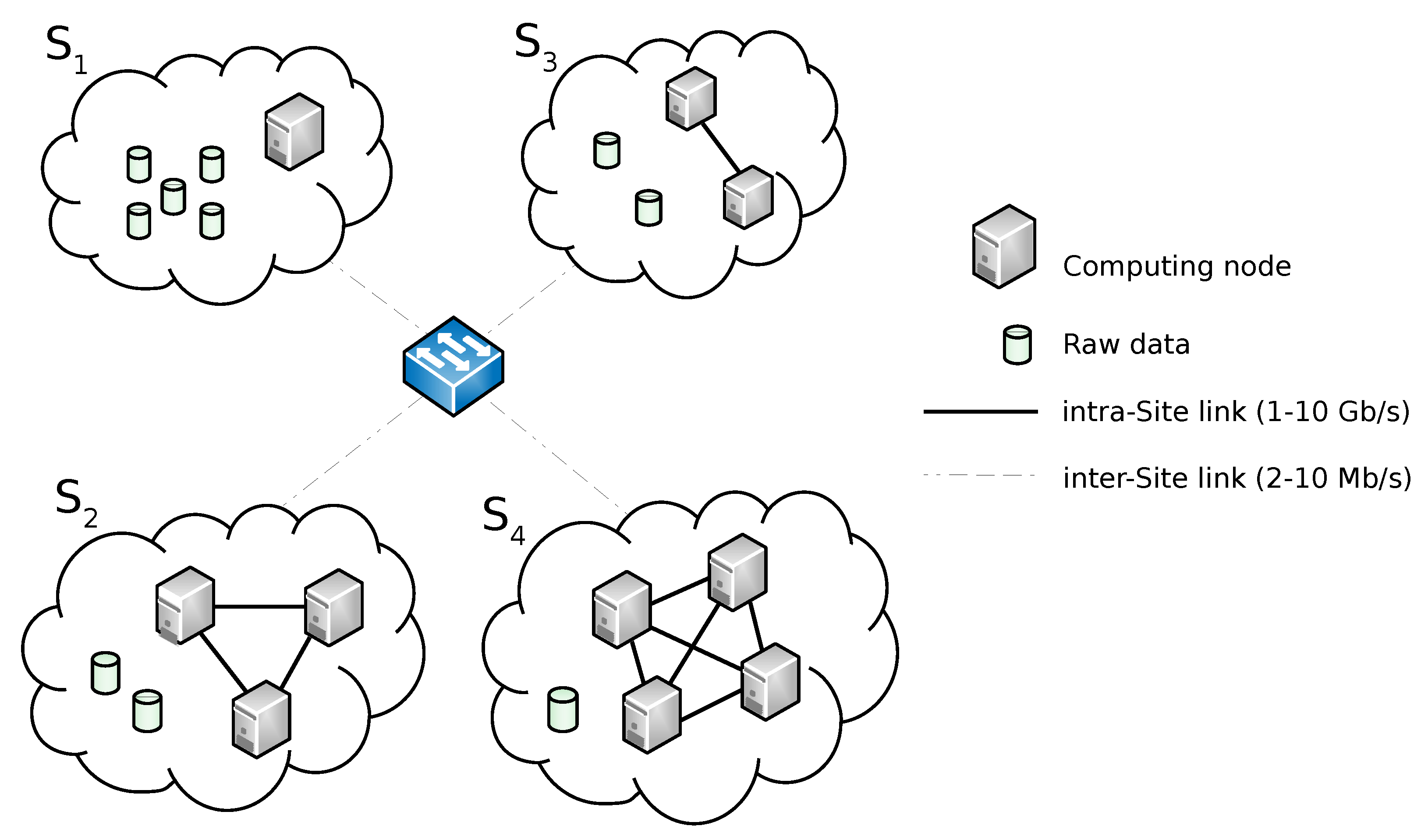
  • Context of the computing scenario. The context encompasses elements such as (a) the number and the capability of the available computing nodes, (b) the topology of the network interconnecting the computing nodes as well as the bandwidth available at each network link, and (c) the amount of data residing at each node involved in the computation.
  • Job scheduling objective. The objective of the scheduling algorithm (optimization of cost, execution time, etc.).
  • Application profiling. Each job encapsulates a specific application that elaborates data according to a given algorithm. The application profile is the “fingerprint” of the application that captures the way the application behaves in terms of data manipulation.
  • Compatibility with MapReduce frameworks. This refers to the possibility of reusing existing software frameworks specifically designed for clusters of close nodes.
  • Data fragmentation. It refers to the opportunity of the fragmenting data of a data center into smaller pieces (blocks) and migrating groups of them to other data centers.
Table 5. Literature review: a comparative analysis.
Computing ContextJob Scheduling ObjectiveApplication ProfilingDeveloped SoftwareCompatibility with MapReduce FrameworksData Fragmentation
Kim et al. [23]CPUMakespan-Hadoop Extension--
Wang et al. [28]-Makespan, Network usage-Hadoop Extension--
Mattess et al. [24]-Monetary cost-Hadoop Extension--
Heinz et al. [7]-Map execution timeMap phaseHadoop Extension--
Zhang et al. [10]-Makespan-Hadoop Extension--
Fahmy et al. [25]-Makespan, Network usage-HDFS ExtensionHadoop 0.20-
You et al. [29]CPUMakespan-Hadoop Extension--
Cheng et al. [31]CPUMakespan-Hadoop Extension--
Li et al. [30]Network, DataMakespan-Hadoop Extension--
Convolbo et al. [32]DataMakespan-Hadoop Extension--
Yu et al. [33]DataMakespan-Simulator--
Luo et al. [11]CPU, DataMakespan-Hadoop Extension--
Jayalath et al. [12]Network, DataMakespan, Monetary cost-Software prototypeHadoopYes
Yang et al. [13]DataMakespan-Software prototype--
H2FCPU, Network, DataMakespanMapReduceSoftware prototypeHadoop (any version)Yes
Though most of the works have taken the computing context in some consideration, only the H2F claims the importance of considering the joint impact of the three aspects: computing resources, network topology/links and data distribution. Among the revised works, only one [7] has considered the opportunity of profiling the application and feeding the job scheduler with the derived profile. Unlike [7], which focuses just on the Map part of the application, our profiling mechanism addresses the MapReduce application’s algorithm as a whole. The main distinctive feature of the solution we propose is the capability of smartly fragmenting and distributing data before the actual computation begins. Jayalath et al. [12] also introduce data fragmentation in their work, but H2F is capable of dealing with data granularity in a much more flexible way: the experiments discussed before have demonstrated that a good guess on the right level of data granularity may positively impact the job’s overall performance. Finally, the H2F software prototype is compatible with any of the available Hadoop frameworks and the like. In fact, the job’s scheduler business logic is fully independent of the specific parallel processing framework running at each Site involved in the distributed computation.

7. Conclusions and Final Remarks

The gradual increase in the amount of information produced daily by devices connected to the Internet, combined with the huge volume of data residing in traditional databases, has led to the definition of the Big Data concept. MapReduce is probably the most famous paradigm widely used in both academic and commercial contexts to run parallel computation on Big Data. However, when it comes to computing data natively scattered over multiple and heterogeneous computing resources, MapReduce fails to guarantee acceptable performance.
This paper discusses a proposal of a hierarchical computing framework that leverages a novel data fragmentation technique to improve the performance of parallel computation in geographically distributed contexts.
More specifically, we developed a context-aware scheduler that explores a significant spectrum of job schedules (execution paths) and comes up with a sub-optimal, yet very efficient solution. In the study presented in this paper, the scheduler seeks for the sub-optimal data block size by exploring a sub-set of viable data block size values. If on the one hand data fragmentation adds further complexity to scheduling process, on the other hand the fragmentation increases the chance of parallelizing the tasks of a given Job. Taking a close look at the results, it can be noticed that with larger block sizes longer job completion, times are observed. We remark that the data fragmentation and distribution scheme produced by the scheduler is always the result of a compromise between the opportunity of exploiting the most powerful computing resources and the constraint imposed by the worst-performing network links. The study proved that, in imbalanced computing environments, an accurate plan of data fragmentation and redistribution among the involved computing resources improves the performance of MapReduce jobs.
In the future, we will work on the design and implementation of a new component responsible for the management of the data replicas that circulate in the distributed computing scenario. By tracing the movement and the position of data and their replicas, we are confident that more performing job schedules may be devised. Furthermore, we plan to run experiments on a geographically scaled testbed. In particular, we are tackling the design of a controlled distributed environment built upon several proprietary infrastructures (computing resources, networking elements and geographic links) offered by public Cloud providers.

Author Contributions

Conceptualization, methodology and software, G.D.M. and O.T.; writing—review and editing, G.D.M. and O.T. All authors have read and agreed to the published version of the manuscript.

Funding

This research received no external funding.

Institutional Review Board Statement

Not applicable.

Informed Consent Statement

Not applicable.

Conflicts of Interest

The authors declare no conflict of interest.

References

  1. Jin, X.; Wah, B.W.; Cheng, X.; Wang, Y. Significance and Challenges of Big Data Research. Big Data Res. 2015, 2, 59–64. [Google Scholar] [CrossRef]
  2. Kambatla, K.; Kollias, G.; Kumar, V.; Grama, A. Trends in big data analytics. J. Parallel Distrib. Comput. 2014, 74, 2561–2573. [Google Scholar] [CrossRef]
  3. Hashem, I.A.T.; Yaqoob, I.; Anuar, N.B.; Mokhtar, S.; Gani, A.; Khan, S.U. The rise of “big data” on cloud computing: Review and open research issues. Inf. Syst. 2015, 47, 98–115. [Google Scholar] [CrossRef]
  4. Pääkkönen, P.; Pakkala, D. Reference Architecture and Classification of Technologies, Products and Services for Big Data Systems. Big Data Res. 2015, 2, 166–186. [Google Scholar] [CrossRef] [Green Version]
  5. Hilty, L.M.; Aebischer, B. ICT for Sustainability: An Emerging Research Field. In ICT Innovations for Sustainability; Springer International Publishing: Berlin/Heidelberg, Germany, 2015; pp. 3–36. [Google Scholar] [CrossRef] [Green Version]
  6. Cardosa, M.; Wang, C.; Nangia, A.; Chandra, A.; Weissman, J. Exploring MapReduce Efficiency with Highly-Distributed Data. In Proceedings of the Second International Workshop on MapReduce and Its Applications, San Jose, CA, USA, 8 June 2011; Association for Computing Machinery: New York, NY, USA, 2011; pp. 27–34. [Google Scholar] [CrossRef] [Green Version]
  7. Heintz, B.; Chandra, A.; Sitaraman, R.; Weissman, J. End-to-end Optimization for Geo-Distributed MapReduce. IEEE Trans. Cloud Comput. 2016, 4, 293–306. [Google Scholar] [CrossRef]
  8. Dean, J.; Ghemawat, S. MapReduce: Simplified data processing on large clusters. In Proceedings of the 6th Conference on Symposium on Operating Systems Design and Implementation, USENIX Association, OSDI’04, San Francisco, CA, USA, 6–8 December 2004. [Google Scholar]
  9. The Apache Software Foundation. The Apache Hadoop Project. 2011. Available online: hadoop.apache.org (accessed on 29 December 2021).
  10. Zhang, Q.; Liu, L.; Lee, K.; Zhou, Y.; Singh, A.; Mandagere, N.; Gopisetty, S.; Alatorre, G. Improving Hadoop Service Provisioning in a Geographically Distributed Cloud. In Proceedings of the 2014 IEEE 7th International Conference on Cloud Computing (CLOUD’14), Anchorage, AK, USA, 27 June–2 July 2014; pp. 432–439. [Google Scholar] [CrossRef] [Green Version]
  11. Luo, Y.; Guo, Z.; Sun, Y.; Plale, B.; Qiu, J.; Li, W.W. A Hierarchical Framework for Cross-domain MapReduce Execution. In Proceedings of the Second International Workshop on Emerging Computational Methods for the Life Sciences (ECMLS ’11), Trento, Italy, 29 September–1 October 2011; pp. 15–22. [Google Scholar] [CrossRef]
  12. Jayalath, C.; Stephen, J.; Eugster, P. From the Cloud to the Atmosphere: Running MapReduce across Data Centers. IEEE Trans. Comput. 2014, 63, 74–87. [Google Scholar] [CrossRef]
  13. Yang, H.; Dasdan, A.; Hsiao, R.; Parker, D.S. Map-reduce-merge: Simplified Relational Data Processing on Large Clusters. In Proceedings of the 2007 ACM SIGMOD International Conference on Management of Data (SIGMOD’07), Beijing, China, 11–14 June 2017; pp. 1029–1040. [Google Scholar] [CrossRef]
  14. Cavallo, M.; Di Modica, G.; Polito, C.; Tomarchio, O. H2F: A Hierarchical Hadoop Framework for big data processing in geo-distributed environments. In Proceedings of the 3rd IEEE/ACM International Conference on Big Data Computing, Applications and Technologies (BDCAT 2016), Shanghai, China, 6–9 December 2016; pp. 27–35. [Google Scholar] [CrossRef]
  15. Cavallo, M.; Di Modica, G.; Polito, C.; Tomarchio, O. Fragmenting Big Data to boost the performance of MapReduce in geographical computing contexts. In Proceedings of the 3rd International Conference on Big Data Innovations and Applications (Innovate-Data 2017), Prague, Czech Republic, 21–23 August 2017; pp. 17–24. [Google Scholar] [CrossRef]
  16. Facebook. Project PRISM. 2012. Available online: www.wired.com/2012/08/facebook-prism (accessed on 29 December 2021).
  17. Dastjerdi, A.V.; Gupta, H.; Calheiros, R.N.; Ghosh, S.K.; Buyya, R. Fog Computing: Principles, architectures, and applications. In Internet of Things: Principles and Paradigms; Morgan Kaufmann: Burlington, MA, USA, 2016; pp. 61–75. [Google Scholar] [CrossRef] [Green Version]
  18. Cavallo, M.; Di Modica, G.; Polito, C.; Tomarchio, O. Application Profiling in Hierarchical Hadoop for Geo-distributed Computing Environments. In Proceedings of the IEEE Symposium on Computers and Communications (ISCC 2016), Messina, Italy, 27–30 June 2016; pp. 555–560. [Google Scholar] [CrossRef]
  19. Cavallo, M.; Di Modica, G.; Polito, C.; Tomarchio, O. A LAHC-based Job Scheduling Strategy to Improve Big Data Processing in Geo-distributed Contexts. In Proceedings of the 2nd International Conference on Internet of Things, Big Data and Security (IoTBDS 2017), Porto, Portugal, 24–26 April 2017; pp. 92–101. [Google Scholar] [CrossRef]
  20. Zhao, L.; Yang, Y.; Munir, A.; Liu, A.X.; Li, Y.; Qu, W. Optimizing Geo-Distributed Data Analytics with Coordinated Task Scheduling and Routing. IEEE Trans. Parallel Distrib. Syst. 2020, 31, 279–293. [Google Scholar] [CrossRef]
  21. Huang, Y.; Shi, Y.; Zhong, Z.; Feng, Y.; Cheng, J.; Li, J.; Fan, H.; Li, C.; Guan, T.; Zhou, J. Yugong: Geo-Distributed Data and Job Placement at Scale. Proc. VLDB Endow. 2019, 12, 2155–2169. [Google Scholar] [CrossRef]
  22. Oh, K.; Chandra, A.; Weissman, J. A Network Cost-aware Geo-distributed Data Analytics System. In Proceedings of the 20th IEEE/ACM International Symposium on Cluster, Cloud and Internet Computing (CCGRID 2020), Melbourne, Australia, 11–14 May 2020; pp. 649–658. [Google Scholar] [CrossRef]
  23. Kim, S.; Won, J.; Han, H.; Eom, H.; Yeom, H.Y. Improving Hadoop Performance in Intercloud Environments. SIGMETRICS Perform. Eval. Rev. 2011, 39, 107–109. [Google Scholar] [CrossRef]
  24. Mattess, M.; Calheiros, R.N.; Buyya, R. Scaling MapReduce Applications Across Hybrid Clouds to Meet Soft Deadlines. In Proceedings of the 2013 IEEE 27th International Conference on Advanced Information Networking and Applications (AINA’13), Barcelona, Spain, 25–28 March 2013; pp. 629–636. [Google Scholar] [CrossRef]
  25. Fahmy, M.M.; Elghandour, I.; Nagi, M. CoS-HDFS: Co-locating Geo-distributed Spatial Data in Hadoop Distributed File System. In Proceedings of the 3rd IEEE/ACM International Conference on Big Data Computing, Applications and Technologies (BDCAT 2016), Shanghai, China, 6–9 December 2016; pp. 123–132. [Google Scholar] [CrossRef]
  26. Afrati, F.; Dolev, S.; Sharma, S.; Ullman, J. Meta-MapReduce: A Technique for Reducing Communication in MapReduce Computations. In Proceedings of the 17th International Symposium on Stabilization, Safety, and Security of Distributed Systems (Springer-SSS), Edmonton, AB, Canada, 18–21 August 2015. [Google Scholar]
  27. He, C.; Weitzel, D.; Swanson, D.; Lu, Y. HOG: Distributed Hadoop MapReduce on the Grid. In Proceedings of the 2012 SC Companion: High Performance Computing, Networking Storage and Analysis, Salt Lake City, UT, USA, 10–16 November 2012; pp. 1276–1283. [Google Scholar] [CrossRef] [Green Version]
  28. Wang, L.; Tao, J.; Ranjan, R.; Marten, H.; Streit, A.; Chen, J.; Chen, D. G-Hadoop: MapReduce across distributed data centers for data-intensive computing. Future Gener. Comput. Syst. 2013, 29, 739–750. [Google Scholar] [CrossRef]
  29. You, H.H.; Yang, C.C.; Huang, J.L. A Load-aware Scheduler for MapReduce Framework in Heterogeneous Cloud Environments. In Proceedings of the 2011 ACM Symposium on Applied Computing (SAC 2011), TaiChung, Taiwan, 21–24 March 2011; pp. 127–132. [Google Scholar] [CrossRef]
  30. Li, P.; Guo, S.; Miyazaki, T.; Liao, X.; Jin, H.; Zomaya, A.Y.; Wang, K. Traffic-Aware Geo-Distributed Big Data Analytics with Predictable Job Completion Time. IEEE Trans. Parallel Distrib. Syst. 2017, 28, 1785–1796. [Google Scholar] [CrossRef]
  31. Cheng, D.; Rao, J.; Guo, Y.; Jiang, C.; Zhou, X. Improving Performance of Heterogeneous MapReduce Clusters with Adaptive Task Tuning. IEEE Trans. Parallel Distrib. Syst. 2017, 28, 774–786. [Google Scholar] [CrossRef]
  32. Convolbo, M.W.; Chou, J.; Lu, S.; Chung, Y.C. DRASH: A Data Replication-Aware Scheduler in Geo-Distributed Data Centers. In Proceedings of the 2016 IEEE International Conference on Cloud Computing Technology and Science (CloudCom), Luxembourg, 12–15 December 2016; pp. 302–309. [Google Scholar] [CrossRef]
  33. Yu, B.; Pan, J. Location-aware associated data placement for geo-distributed data-intensive applications. In Proceedings of the 2015 IEEE Conference on Computer Communications (INFOCOM 2015), Kowloon, Hong Kong, 26 April–1 May 2015; pp. 603–611. [Google Scholar] [CrossRef]
  34. Dolev, S.; Florissi, P.; Gudes, E.; Sharma, S.; Singer, I. A Survey on Geographically Distributed Big-Data Processing using MapReduce. IEEE Trans. Big Data 2019, 5, 60–80. [Google Scholar] [CrossRef] [Green Version]
  35. Bergui, M.; Najah, S.; Nikolov, N.S. A survey on bandwidth-aware geo-distributed frameworks for big-data analytics. J. Big Data 2021, 8, 1–26. [Google Scholar] [CrossRef]
Figure 1. Motivating scenario.
Bdcc 06 00005 g001
Figure 3. Overall architecture.
Bdcc 06 00005 g003
Figure 4. Reference scenario.
Bdcc 06 00005 g004
Figure 5. Multi-job scheduling.
Bdcc 06 00005 g005
Figure 6. Nodes and queue in the job’s execution path model.
Bdcc 06 00005 g006
Figure 8. Example topology with 3 Sites.
Bdcc 06 00005 g008
Figure 9. Reference topology.
Bdcc 06 00005 g009
Figure 10. First battery of tests: results from the scenarios where data are evenly distributed among Sites.
Bdcc 06 00005 g010
Figure 11. Second battery of tests: results from the scenarios where overall data are initially placed in S 4 .
Bdcc 06 00005 g011
Figure 12. Third battery of tests: results from the scenarios where data are initially placed on Sites S 1 and S 3 .
Bdcc 06 00005 g012
Figure 13. Network topology of test-bed environment.
Bdcc 06 00005 g013
Figure 14. H2F vs. Hadoop: comparison of job’s execution time for (a) C o n f i g 1 , (b) C o n f i g 2 and (c) C o n f i g 3 in the 5 GB raw data scenario.
Bdcc 06 00005 g014
Figure 15. H2F vs. Hadoop: comparison of job’s execution time for (a) C o n f i g 1 , (b) C o n f i g 2 and (c) C o n f i g 3 in the 50 GB raw data scenario.
Bdcc 06 00005 g015
Figure 16. H2F vs. Hadoop: comparison of job’s execution time for (a) C o n f i g 4 and (b) C o n f i g 5 .
Bdcc 06 00005 g016
Table 1. Configurations used for the tests.
Sites [GFLOPS]Links [MB/s]
Config S 1 S 2 S 3 S 4 S 5 S 6 L 1 L 2 L 3 L 4 L 5 L 6
1505050505050101010101010
2502550255025101010101010
3505050505050510510510
4255025502550105105105
5502550255025105105105
Table 2. Nominal block Size computed for the five configurations.
Config 1 Config 2 Config 3 Config 4 Config 5
N o m i n a l B l o c k S i z e 1.67 GB1.38 GB1.52 GB1.52 GB1.24 GB
Table 3. Configurations of the data blocks’ distribution.
S 1 S 2 S 3 S 4
C o n f i g 1 40%30%20%10%
C o n f i g 2 40%40%20%0%
C o n f i g 3 30%0%70%0%
Table 4. Links’ Configurations.
L 1   [ MB / s ] L 2   [ MB / s ] L 3   [ MB / s ] L 4   [ MB / s ]
C o n f i g 4 20204040
C o n f i g 5 20402040
Publisher’s Note: MDPI stays neutral with regard to jurisdictional claims in published maps and institutional affiliations.

