Clustering Algorithm to Measure Student Assessment Accuracy: A Double Study

Abstract

Self-assessment is one of the strategies used in active teaching to engage students in the entire learning process, in the form of self-regulated academic learning. This study aims to assess the possibility of including self-evaluation in the student’s final grade, not just as a self-assessment that allows students to predict the grade obtained but also as something to weigh on the final grade. Two different curricular units are used, both from the first year of graduation, one from the international relations course (N = 29) and the other from the computer science and computer engineering courses (N = 50). Students were asked to self-assess at each of the two evaluation moments of each unit, after submitting their work/test and after knowing the correct answers. This study uses statistical analysis as well as a clustering algorithm (K-means) on the data to try to gain deeper knowledge and visual insights into the data and the patterns among them. It was verified that there are no differences between the obtained grade and the thought grade by gender and age variables, but a direct correlation was found between the thought grade averages and the grade level. The difference is less accentuated at the second moment of evaluation—which suggests that an improvement in the self-assessment skill occurs from the first to the second evaluation moment.

1. Introduction

The teaching–learning process is more efficient as the student is integrated in all phases. Thus, the student becomes an active member and not a mere spectator of a process in which the teacher is solely responsible. Student-centered instruction involves students throughout the process. Evaluation is a very important part; it is a very serious task that requires the use of rigid correction grids. Assessment is used as a measure of knowledge and is part of the teaching–learning process. So, if students are to be involved in the entire process, they must also be active elements in this task.

Are all students capable of self-assessment? Are there characteristics in students that allow them to have better or worse self-assessment skills? The main reason for this study is to know how and if it is possible to involve students in their own assessment in a fair and formal way. We also tried to find out if there are some characteristics of students that make the perception of their own level of knowledge coincide or not with the teacher’s perception.

This article describes an experiment carried out in two different curricular units of two different types of course, with two evaluation moments each. It was performed by asking students to evaluate the work or test delivered according to the teacher’s correction grid, on a scale from 0 to 20 values. As a measure, the DOT (difference between the grade obtained and the student’s thinking, explained in Section 3.3) was used for each moment of assessment and course and was analyzed by gender, age, and grade level obtained.

This article is divided into Review of Literature, Methodology (data collection, population, measures, and clustering), Results, Discussion of Results, and Conclusions.

2. Review of Literature

It is important, in a research study, to review the current and available literature to understand the issues related with the insertion strategies of the student as an integral and active part of teaching–learning, namely as a participant in their own assessment. In this section we approach student-centered instruction, self-regulated academic learning, self-assessment, and self-evaluation.

2.1. Student-Centered Instruction

Constructivist learning theory directs towards learning as an active process in which students are active sense makers who seek to build coherent and organized knowledge [1]. It becomes student-centered learning because it emphasizes student responsibility and activity in learning rather than what the teachers are doing [2], and the learning process is done by engaging in and interacting with the study material guided by the teacher. While in the traditional approach to higher education, the burden of communicating course material resides mainly with the instructor, in student-centered instruction, part of this load is transferred to the students [3]. To be effective, student-centered teaching methods require student independence and a change from the traditional role of the teacher to coaching roles, which is very different from the act of transmitting knowledge. According to Agustini et al., there are three conditions that make student-centered learning models more effective: (1) the existence of modeling (involving behavior modeling activities to encourage performance development and cognitive modeling to encourage cognitive processes), (2) the existence of training (in the sense of coaching, which involves providing motivation, monitoring and regulating student activities, and encouraging students to reflect themselves), and (3) the presence of scaffolding (concerning the activities of providing support and/or assistance temporally according to the capacity of the learners’ abilities, including determining the level of difficulty of the task, restructuring tasks, and providing alternative assessments) [4]. Students are involved in higher order thinking tasks, such as analysis, synthesis, and evaluations, involving students in doing things and thinking about what they are doing [5]. Student-centered learning can take different forms, often appearing in practices such as project-based learning, collaborative learning, and technology-enhanced learning, which operationalize student-centeredness [6].

2.2. Self-Regulated Academic Learning

Self-regulated academic learning emerged in the 1980s with the prospect that students become masters of their own learning process [7] and it can be designed as a cyclical process that repeats itself, in which planning tasks and reflection on the outcome are used in preparation for the next task [8] or alternatively anticipation, monitoring, control, and reflection [9]. Urbina et al. [10] listed the five most used models in the literature and their assessment strategies: Bandura’s social-cognitive model [11], Boekaerts’s Heuristic Model [12], Winne and Hadwin [13], Pintrich Model [9], and Zimmerman’s cyclical model [8]. Self-regulated learning is generally understood as having a phased process with a forethought phase, a performance phase, and a self-reflection phase [14]. Intelligent self-regulation requires a clear definition of the objectives that are to be achieved. The performance can be compared and evaluated in relation to these objectives, including its specific goals, criteria, and standards that help set goals [15]. There are several skills that students need to develop, some of which are largely dependent on the ability of individuals to be self-reflective [16]. Due assessment is a very important part of the system and is used as a measure to assess students’ knowledge, above all following a positivist perspective. Three types of assessment are identified: (1) diagnostic (identifying the level of prior knowledge to be compared with the learning objectives), (2) formative (used for decision making in the teaching–learning process, such as moving to the next objective), and (3) summative assessment (at the end of the course, to make decisions about the performance achieved by students, often with the attribution of grades) [17]. So, formative assessment provides information for students about their progress, while summative assessment provides the student with final achievement information [18].

2.3. Self-Assessment

According to Bound [19], assessment is most effective when it is used to engage students in learning and when it is recognized as a learning activity and students progressively take responsibility for assessment and feedback processes. Self-assessment can be defined as the involvement of students in making judgments of their learning [20]. Self-assessment can also be defined as a tool to build the metacognition of the learners, enhancing the knowledge of the learner about their own learning, increasing students’ motivation, commitment, and responsibility [21]. Metacognition describes the various aspects of how a learner processes new knowledge with the explicit understanding and recognition that learning is taking place [22]. Savin-Baden [23] emphasizes the need for self-assessment and peer assessment to be considered by universities, thus making this task more serious for students and assessors. In the literature there are many reports of experience with Self, Peer, and Teacher Assessments. For an effective self-assessment, it is necessary to diversify assessment instruments, decentralize assessment moments, adapt the form of assessment to the type of skill or competence to be assessed, clarify student assessment criteria, and use instruments of evaluation [24]. The problem of students’ perception of results is investigated by several authors. According to Adams [25], students consistently believed that effort should account for much more in the final grade than the faculty. Remedios et al. [26] show how important it is to distinguish between aspirations and expectations of grades: the grades students hope to achieve and the realistic versions of the grades, respectively. In a study with 11th grade students [27], it was found that 90% self-assessed themselves at levels higher than the evaluator, suggesting that students are not familiar with self-assessment and because they trust the teacher as the only one evaluator of its performance. Another study with university students reveals that students with higher performance and more involvement tend to show greater skills with self-assessment; and students with better study habits tend to have better scores, greater confidence, and better self-assessment skills [28]. A study with peer assessment and self-assessment of group work in a computer programming unit reveals that the more students know, the more they think they do not know, and the less they know, the more ignorance they have about their knowledge [29]. Unskilled and unaware, they are doubly cursed: they have no knowledge of the material and they are unaware of the knowledge they (do not) possess [30]. An effort has been made to characterize these behaviors in terms of various variables, such as gender differences [31,32] or not [22], or being a freshman student [33] or not [34]. There are studies that publish suggestions on how to improve the self-regulation capacity of students: Belski and Belski [35] suggest regularly involving students in the forecasting process, helping them to regularly practice diagnostic self-assessment and reflection on their learning. In the same way, Thawabieh [36] believes that students’ ability to self-assess can be improved if they are trained to implement self-assessment. Calibration is calculated by taking the difference between self-assessment and performance [37,38].

2.4. Self-Evaluation

Sullivan and Hall [39] have distinguished between the broader process of “self-evaluation” and the strategy of “self-assessment”. It is important to make a distinction between assessment (measuring quality, value, or importance; used for level of performance) and evaluation (judgment on values, numbers, or performance; used to determine degree). In several languages the same word is being used for both concepts (for example, in Portuguese the word “avaliação” is used, in Spanish it is “evaluación”, and in French it is “évaluation”).

One of the objectives of this study is precisely this: to verify whether self-assessment can be considered in the teaching–learning process and whether the difference between the grade obtained by the student and the grade that the student expects to obtain is correlated with different variables and, if so, which of the variables have a greater correlation to it.

3. Methodology

In this section we approach four topics: in Section 3.1 we explain the data acquisition process, including a description of the courses and curricular units in which the study was performed; in Section 3.2 we describe the study participants, that is, the students enrolled in each of the considered curricular units; in Section 3.3 we explain the measures used for the study, as well as the grading system in Portugal, and in Section 3.4 we describe the clustering method applied to the data.

3.1. Data Acquisition

This study is based on two distinct curricular units, both in the first year of undergraduate courses. The first one is aimed at International Relations students (Unit A) and the other at Computer Science and Computer Engineering students (Unit B). Both courses have 80% of the final grade due to two assessment moments, with the remaining 20% associated with semester assignments and small assessment questionnaires. In both curricular units, the students were asked to voluntarily complete a survey. The survey link was available on the MOODLE page and the survey was prepared in Google Forms. In this survey, among other questions, the year of birth, gender, and student number are asked. The objective of the student number variable is to relate the survey’s answers to the students’ grades. The remaining variables are the ones that this study aims to relate to the students’ grades. Due to being a voluntary activity, the request to fill out the survey was made several times, with the objective of having as much data as possible.

The self-assessment process for each assessment moment consists in providing the students with the evaluation criteria and grid (with the weight considered for each criterium) and asking them to rate their work with a percentage (0–100%) for each evaluation criteria. With this, we obtain the students’ self-assessment: their predicted grades (in a scale of 0–20) for that assessment moment.

For clarification, the grades of students in Portugal ranged from 0 to 20 values. Students with a grade below 9.5 fail the test, while students with grades of 9.5 or higher pass the test. In this study we consider four ranges for the grades: low-negative (below 5 values: $\left[0,5\right]$), negative (between 5 and 10 values: $\left[5,10\right[$), positive (between 10 and 15 values: $\left[10,15\right[$), and high-positive (over 15 values: $\left[15,20\right]$).

Each of the two evaluation moments of Unit A consisted of a paper submitted and its presentation, which included several digital tools such as Google Forms, MS Office, and bibliographic management. Students’ self-assessment was performed after the submission of each work and before the individual presentation. The self-assessment was also used as a basis for teacher-to-student questions during the work presentation.

In Unit B, each assessment moment was a test which consisted in a written part (algorithms) and a program (in C for computer science students, and in Python for Computer Engineering students). Students’ self-assessment was performed at the end of the test.

In this study, we consider only the data of students who completed the initial survey, attended the two assessment moments, and responded to the self-assessment for both moments.

3.2. Participants

Due to privacy concerns, the surveys are voluntary. This causes the number of replies to be low, making the number of students eligible for the study low as well.

According to the eligibility criteria mentioned in the previous subsection (the students considered for the study are those who answered the initial survey, attended the two assessment moments, and completed the self-assessment for each evaluation moment), not all students were considered for this study. Next, we describe the ones that were considered. For the first assessment moment the average grade was 12.14, and for the second assessment moment it was 12.16.

In Unit A, 29 students were considered: 24 students are female, and 5 are male. Besides, 12 students were 18 years old, and 17 students were over 18 years old. For the first assessment moment the average grade was 9.34, and for the second assessment moment it was 7.86.

3.3. Measures

The measure used in this study, which we call DOT, is the difference between the grade obtained at the assessment and the student’s self-assessment. DOT is obtained by subtracting the grade predicted by the student in self-assessment from the obtained grade ($DOT=grad{e}_{self-assessment}-grad{e}_{obtained}$). For example, let us consider two students: the first student self-assessed his grade to be 17.83, but the actual test grade was 16.98—the student over-assessed his work, and his DOT is −0.85; the second student self-assessed his grade to be 16.60, but the actual test grade was 16.81—the student under-assessed his work, and his DOT is 0.21.

In the statistical analysis, the p-value, or probability value, was used, which is a number that describes the probability of the null hypothesis being true, that is, the data occurred so randomly. The p-value is between 0 and 1; the smaller it is, the stronger the evidence that the null hypothesis should be rejected. In this case, we consider the null hypothesis ($H_0$) to be “the grades occurred randomly”. Low values for the p-value indicate that the null hypothesis should be rejected, which is: the grades did not occur randomly.

We have also performed a t-test analysis, considering the null hypothesis to be $H_0:\mu =0$(the average DOT is 0, meaning that the students accurately self-assess their work) and the alternative hypothesis to be $H_1:\mu \ne 0$ (the average DOT is not 0, meaning that the students cannot accurately self-assess their work.

For the clustering with k-means results, the metric used for evaluation is the Sum of Squared Errors (SSE), which measures the variation within the cluster, by obtaining the distance of each cluster element to its centroid. This metric is obtained by $SSE={\displaystyle \sum }_{i=1}^n{\left(x_i-\overline{x}\right)}^2$, where $n$ is the number of elements in the dataset, $x_i$ represents each element of the dataset, and $\overline{x}$ represents the centroid of the cluster $x_i$ was assigned to. Lower SSE values mean that the elements of each cluster are close together, while higher values mean that the elements are more disperse.

3.4. Clustering

Besides the statistical analysis, clustering was also applied to the data in two different ways. The objective of using clustering is to try to acquire deeper knowledge and visual insights on the data and the patterns among it, trying to analyze the magnitude and direction of the difference between the obtained and the self-assessed grades (DOT).

The first clustering was performed in four datasets: one for each curricular unit and evaluation moment. In each dataset, the variables considered were the obtained grade, the self-assessed grade, and the DOT. As the values are all continuous, the chosen algorithm was the K-means, since it is easily interpretable: the centroids represent the average of the observations in the cluster. The K-means algorithm was run in Python using the scikit-learn library.

We started by defining the number of clusters to be considered. For that, to use the elbow method, we executed the clustering with K varying between 1 and 10 and plotted a chart with the SSE obtained for each K. Figure 1 shows the plot obtained for the first evaluation moment in Unit A. The rest of the datasets have a similar behavior.

With the elbow method, by looking at the plot, we chose the elbow of the curve as K, since using higher values for K will make the algorithm more computational expensive, with low improvement of the SSE. For this reason, the K-means algorithm was executed with K = 3 (3 clusters) for all the datasets.

The second clustering was performed in a single dataset, containing four variables: the DOT, the grade level (low-negative (below 5 values: [0,5]), negative (between 5 and 10 values: [5,10[), positive (between 10 and 15 values: [10,15]), high-positive (over 15 values: [15,20]), the assessment moment (first, or second), and the unit (A, or B). As, in this case, there are categorical values, the chosen algorithm was K-Prototypes, and it was also run in Python. As for the K-means, we started by using the elbow method to choose K, according to the cost function. We plotted the cost function (Figure 2) and, based on the elbow method, chose K to be 3.

4. Results

4.1. Unit A

As mentioned in Section 3.2, in Unit A, for the International Relations course, 29 students were considered. From these, 24 were females and 5 were male; 12 students were 18 years old, and 17 were over 18 years old.

Regarding the grades, two students were graded in the low-negative range (below 5 values), six were graded in the negative range (between 5 and 10 values), thirteen were graded in the positive range (between 10 and 15 values), and eight students were graded in the high-positive range over 15 values out of 20.

The DOT average for the first assessment moment was −3.85, with a standard deviation of 4.13, a minimum of −11.88, and a maximum of 7.5. The DOT average for the second assessment moment was −1.65, with a standard deviation of 2.83, a minimum of −6.59, and a maximum of 3.89. The p-values obtained were 0.000, 0.741, and 0.629 for grade, gender, and age, respectively.

4.2. Unit B

In Unit B, for the Computer Science and Computer Engineering courses, 50 students were considered. From these, 5 were female and 45 were male; 24 students were 18 years old and 26 were over 18 years old.

Regarding the grades, thirteen students were graded in the low-negative range (below 5 values), ten were graded in the negative range (between 5 and 10 values), twenty were graded in the positive range (between 10 and 15 values), and seven students were graded in the high-positive range (over 15 values out of 20).

The DOT average for the first assessment moment was 0.78, with a standard deviation of 2.99, a minimum of −6.9, and a maximum of 7.5. The DOT average for the second assessment moment was −1.75, with a standard deviation of 1.89, a minimum of −5.6, and a maximum of 2.5. The p-values obtained were 0.000, 0.257, and 0.472 for grade, gender, and age, respectively.

4.3. Values

Table 1. Statistical analysis performed for Unit A.

	N1	AVG1	STD1	N2	AVG2	STD2	p-Value
Total	29	−3.85	4.13	29	−1.65	2.83
Grade							0.000
[0–5]	2	−10.94	0.94	1	−6.24	0
[5–10]	6	−7.83	1.63	9	−4.5	1.45
[10–15]	13	−3.55	2.07	8	−1.21	1.18
[15–20]	8	0.4	3.17	11	0.77	1.97
Age							0.741
18 years	12	−4.36	3.63	12	−2.31	3.06
>18 years	17	−3.49	4.42	17	−1.19	2.56
Gender							0.629
F	24	−3.64	4.12	24	−1.36	2.8
M	5	−5.21	3.95	5	−3.5	2.24

and

Table 2. Statistical analysis performed for Unit B.

	N1	AVG1	STD1	N2	AVG2	STD2	p-Value
Total	50	0.78	2.99	50	−1.75	1.89
Grade							0.000
[0–5]	13	−2.95	1.56	15	−2.06	1.17
[5–10]	10	−0.26	1.63	20	−2.65	1.62
[10–15]	20	2.36	1.03	7	−0.53	2.59
[15–20]	7	4.7	1.65	8	0.04	0.85
Age							0.257
18 years	24	1.48	2.54	24	−1.25	2.08
>18 years	26	0.14	3.22	26	−2.2	1.57
Gender							0.472
F	5	0.07	2.64	5	−1.18	2.06
M	45	0.86	3.01	45	−1.81	1.86	1.86

show the statistical analysis performed with data obtained on Units A and B, respectively. Each table shows the number of students assessed on the first assessment moment (N1), the average DOT for the first assessment moment (AVG1), the standard deviation of the DOT for the first assessment moment (STD1), the number of students assessed on the second assessment moment (N2), the average DOT for the second assessment moment (AVG2), the standard deviation of the DOT for the second assessment moment (STD2), and the p-value obtained. In each table, three analysis are performed: (1) by grading range (low-negative (below 5 values: $\left[0,5\right]$), negative (between 5 and 10 values: $\left[5,10\right[$), positive (between 10 and 15 values: $\left[10,15\right[$), high-positive (over 15 values: $\left[15,20\right]$)); (2) by age (18 years old and over 18 years old); and (3) by gender (F: female, and M: male).

4.4. T-Test Results

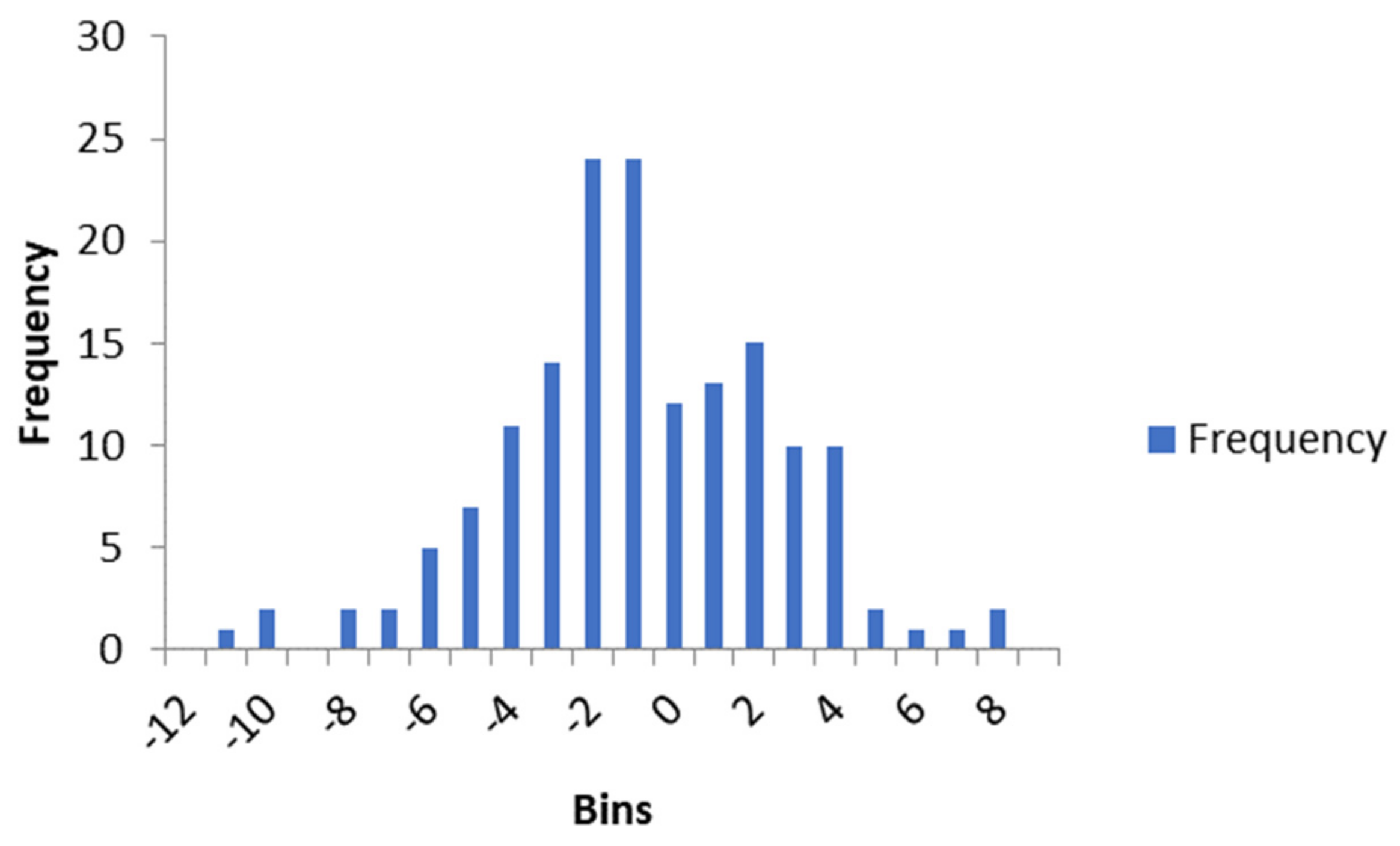
The t-test was performed considering a set of data composed by the DOT for every student of both units, on both assessment moments. There are 158 observations, with average DOT of −1.316 and standard deviation of 3.361. The data’s t value is −4.921. By plotting a histogram of the data (Figure 3), we can see that we need to consider the critical values for the two tailed t distribution table.

With a t value of −4.921, we can state, for this sample with size 158, with 157 degrees of freedom, and a significance of ate least 99.9% ($\alpha =0.001$), that we can reject the null hypothesis ($H_0: \mu =0$), and so, that the students cannot accurately assess their work. In addition, as it is a negative value, students tend to over-assess their work.

We have also performed the t-test for each unit’s assessment moment. These results are presented in

Table 3. Statistics used for the T-test.

	Unit A		Unit B
	First	Second	First	Second
Sample mean	−3.853	−1.654	0.782	−1.745
Sample std. dev	4.207	2.882	3.019	1.912
Nr. obs.	29	29	50	50
t	−4.933	−3.091	1.832	−6.452
Significance	99.9%	99.0%	90.%	99.9%

, which presents, for each unit’s assessment moment, the mean, standard deviation, number of observations, the t value found, and the significance that we can reject the null hypothesis ($H_0: \mu =0$), and so, that the students cannot accurately assess their work.

In Unit A’s first moment, we can state with 99.9% certainty that the students cannot accurately assess their work, and in the second moment we can also state that with 99% certainty. As the t values are negative, we can also state that the students tend do over-assess their work, but that, by the time of the second assessment moment, the difference is lower.

In Unit B we can state, with 90% certainty that the students cannot accurately assess their work, and in the second moment we can state the same with 99.9% certainty. In the first moment, as the t value is greater than zero, we see that students tend to under-assess their work, but on the second moment they tend to over-assess it (as the t value is lower than zero).

4.5. Clustering Results

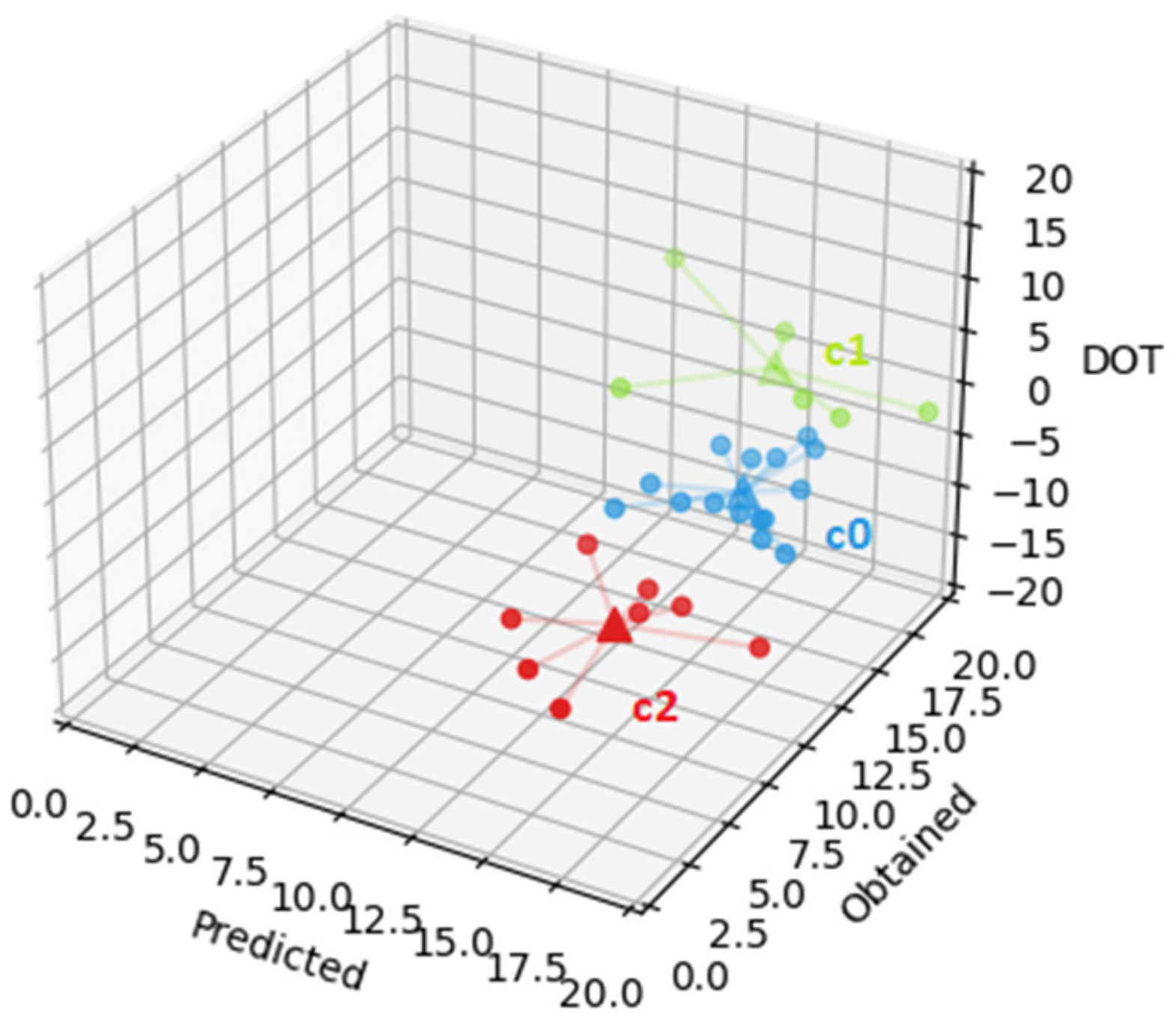
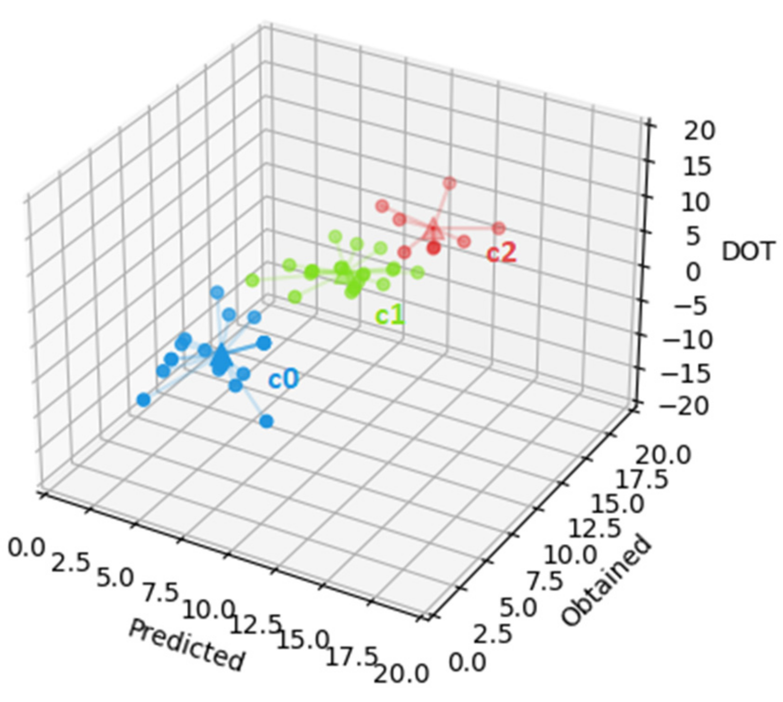
The first clustering was performed using the K-means algorithm in Python, with K = 3. Four different datasets were used: the two assessment moments in each of the two different courses. Each dataset considered three variables: predicted grade, obtained grade, and DOT (the difference between the obtained and the predicted grades). For each dataset, we present a figure and a table. The figure visually represents the clusters found, and the table represents some information available for each cluster (group of students): number of students, cluster SSE, and average and standard deviation of the predicted grade, the obtained grade, and the DOT. In the figures, the circles represent the students, the xx coordinates are each student’s predicted grade on self-assessment, the yy coordinates are each student’s obtained grade, and the zz coordinates are each student’s DOT. Each cluster of students is represented by a different color (blue, green, and red) and the centroid of each cluster is represented by a triangle.

We can see in

Table 4. Statistical representation of the clusters obtained when considering the first test of Unit A.

			Predicted		Obtained		DOT
Cluster	SSE	Nr	Avg	SD	Avg	SD	Avg	SD
0	149.7	15	16.5	1.4	13.0	1.6	−3.6	1.5
1	76.0	6	15.4	3.2	17.2	1.8	1.8	3.0
2	140.4	8	15.4	1.9	6.8	2.1	−8.6	2.0

the information regarding the dataset that considers the first assessment moment for Unit A.

The first cluster (cluster 0, the cluster represented by c0, in blue in Figure 4, with an SSE of 149.7) groups the 15 students with average predicted grade of 16.5 with a standard deviation of 1.4, average obtained grade of 13.0 with standard deviation of 1.6, and average DOT of −3.6 with standard deviation 1.5. The second cluster (cluster 1, the cluster represented by c1, in green in Figure 4, with an SSE of 76.0) groups the 6 students with average predicted grade of 15.4 with standard deviation of 3.2, average obtained grade of 17.2 with standard deviation of 1.8, and average DOT of 1.8 with standard deviation of 3.0. Finally, the third cluster (cluster 2, the cluster represented by c2, in red in Figure 4, with an SSE of 140.4) groups the 8 students with average predicted grade of 15.4 with standard deviation of 1.9, average obtained grade of 6.8 with standard deviation of 2.1, and average DOT of −8.6 with standard deviation of 2.0. Cluster c1 has the lowest SSE, which indicates a higher resemblance among the cluster’s elements. However, in this case, it can also be related to having less students. The most relevant information gathered in this dataset is that students in clusters 1 and 2 predicted, on average, a grade of 15.4. However, students on cluster 1 obtained, on average, a grade of 17.2 with average DOT of 1.8, while students on cluster 2 obtained, on average, a grade of 6.8 with average DOT of −8.6. This shows that students with low grades (as in cluster 2) will predict much higher grades, while students with higher grades will predict slightly lower grades.

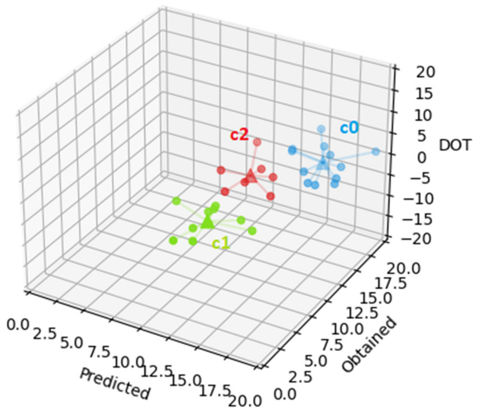
Concerning the second test for Unit A, the results are presented in

Table 5. Statistical representation of the clusters obtained when considering the second test of Unit A.

			Predicted		Obtained		DOT
Cluster	SSE	Nr	Avg	SD	Avg	SD	Avg	SD
0	131.4	12	16.4	2.6	16.5	3.9	0.1	2.9
1	88.6	10	11.6	2.7	6.9	4.7	−4.7	2.6
2	66.0	7	12.4	2.8	12.1	4.9	−0.3	2.9

.

In this case, the first cluster (cluster 0, the cluster represented by c0, in blue in Figure 5, with an SSE of 131.4) groups the 12 students with average predicted grade of 16.4 with a standard deviation of 2.6, average obtained grade of 16.5 with standard deviation of 3.9, and average DOT of 0.1 with standard deviation 2.9. The second cluster (cluster 1, the cluster represented by c1, in green in Figure 5, with an SSE of 88.6) groups the 10 students with average predicted grade of 11.6 with standard deviation of 2.7, average obtained grade of 6.9 with standard deviation of 4.7, and average DOT of −4.7 with standard deviation of 2.6. Finally, the third cluster (cluster 2, the cluster represented by c2, in red in Figure 5, with an SSE of 66.0) groups the 7 students with average predicted grade of 12.4 with standard deviation of 2.8, average obtained grade of 12.1 with standard deviation of 4.9, and average DOT of −0.3 with standard deviation of 2.9. Cluster c2 has the lowest SSE (66.0), followed by cluster c1 (88.6). As the number of students per cluster is more uniform than for the previous results presented, in this case this must indicate a higher resemblance among the elements of each cluster. The most relevant information gathered in this dataset is that students in clusters 0 and 2 have, on average, grades above 10, and their DOT is much lower than that of the students on cluster 1, which obtain, on average, a lower grade. This suggests, on one hand, that students improve their self-assessment by the time of the second test and, on the other hand, that students with lower grades still predict much higher grades than the obtained, although the DOT here is lower than for the first test.

Table 6. Statistical representation of the clusters obtained when considering the first test of Unit B.

			Predicted		Obtained		DOT
Cluster	SSE	Nr	Avg	SD	Avg	SD	Avg	SD
0	240.8	21	6.7	1.5	4.6	1.7	−2.1	1.8
1	152.5	21	9.3	1.5	11.6	1.3	2.3	1.0
2	62.5	8	11.5	1.5	16.0	1.4	4.5	1.6

represents the information regarding the dataset that considers the first test for Unit B.

The first cluster (cluster 0, the cluster represented by c0, in blue in Figure 6, with an SSE of 240.8) groups the 21 students with average predicted grade of 6.7 with a standard deviation of 1.5, average obtained grade of 4.6 with standard deviation of 1.7, and average DOT of −2.1 with standard deviation 1.8. The second cluster (cluster 1, the cluster represented by c1, in green in Figure 6, with an SSE of 152.5) groups the 21 students with average predicted grade of 9.3 with standard deviation of 1.5, average obtained grade of 11.6 with standard deviation of 1.3, and average DOT of 2.3 with standard deviation of 1.0. Finally, the third cluster (cluster 2, the cluster represented by c2, in red in Figure 6, with an SSE of 62.5) groups the 8 students with average predicted grade of 11.5 with standard deviation of 1.5, average obtained grade of 16.0 with standard deviation of 1.4, and average DOT of 4.5 with standard deviation of 1.6. The cluster with the lowest SSE is c2 which, as happened for the clustering of the first assessment for Unit A (Table 3 and Figure 2), can be due to the smaller size of this cluster. The most relevant information gathered in this dataset is that students with very low grades (cluster 0) will predict a slightly higher grade, students with grades slightly above 10 (cluster 1) will predict slightly lower grades, and students with higher grades (cluster 2) will predict lower grades. In addition, when compared to the results for Unit A, the DOT in this case is slightly lower, suggesting a different ability of self-assessment depending on the course.

Finally,

Table 7. Statistical representation of the clusters obtained when considering the second test of Unit B.

			Predicted		Obtained		DOT
Cluster	SSE	Nr	Avg	SD	Avg	SD	Avg	SD
0	47.3	15	4.1	1.5	2.0	0.9	−2.1	1.2
1	396.9	13	15.7	2.6	15.4	2.8	−0.3	1.9
2	297.0	22	9.8	1.2	7.4	1.8	−2.4	1.8

represents the information regarding the dataset that considers the second test for Unit B.

The first cluster (cluster 0, the cluster represented by c0, in blue in Figure 7, with an SSE of 47.3) groups the 15 students with average predicted grade of 4.1 with a standard deviation of 1.5, average obtained grade of 2.0 with standard deviation of 0.9, and average DOT of −2.1 with standard deviation 1.2. The second cluster (cluster 1, the cluster represented by c1, in green in Figure 7, with an SSE of 396.9) groups the 13 students with average predicted grade of 15.7 with standard deviation of 2.6, average obtained grade of 15.4 with standard deviation of 2.8, and average DOT of −0.3 with standard deviation of 1.9. Finally, the third cluster (cluster 2, the cluster represented by c2, in red in Figure 7, with an SSE of 297.0) groups the 22 students with average predicted grade of 9.8 with standard deviation of 1.2, average obtained grade of 7.4 with standard deviation of 1.8, and average DOT of −2.4 with standard deviation of 1.8. Here, cluster c0′s SSE is much lower than the other clusters’ SSE. Again, as happened for the second assessment moment for Unit A (Table 4 and Figure 3), this indicates a higher resemblance between this cluster’s elements. The most relevant information gathered in this dataset is that students with lower grades (clusters 0 and 2) will still predict a slightly higher grade, while students with higher grades (cluster 1) will predict a grade that is very close to the one the students in fact obtained. Besides, as happened in Unit A, by the second test, students have improved their self-assessment ability.

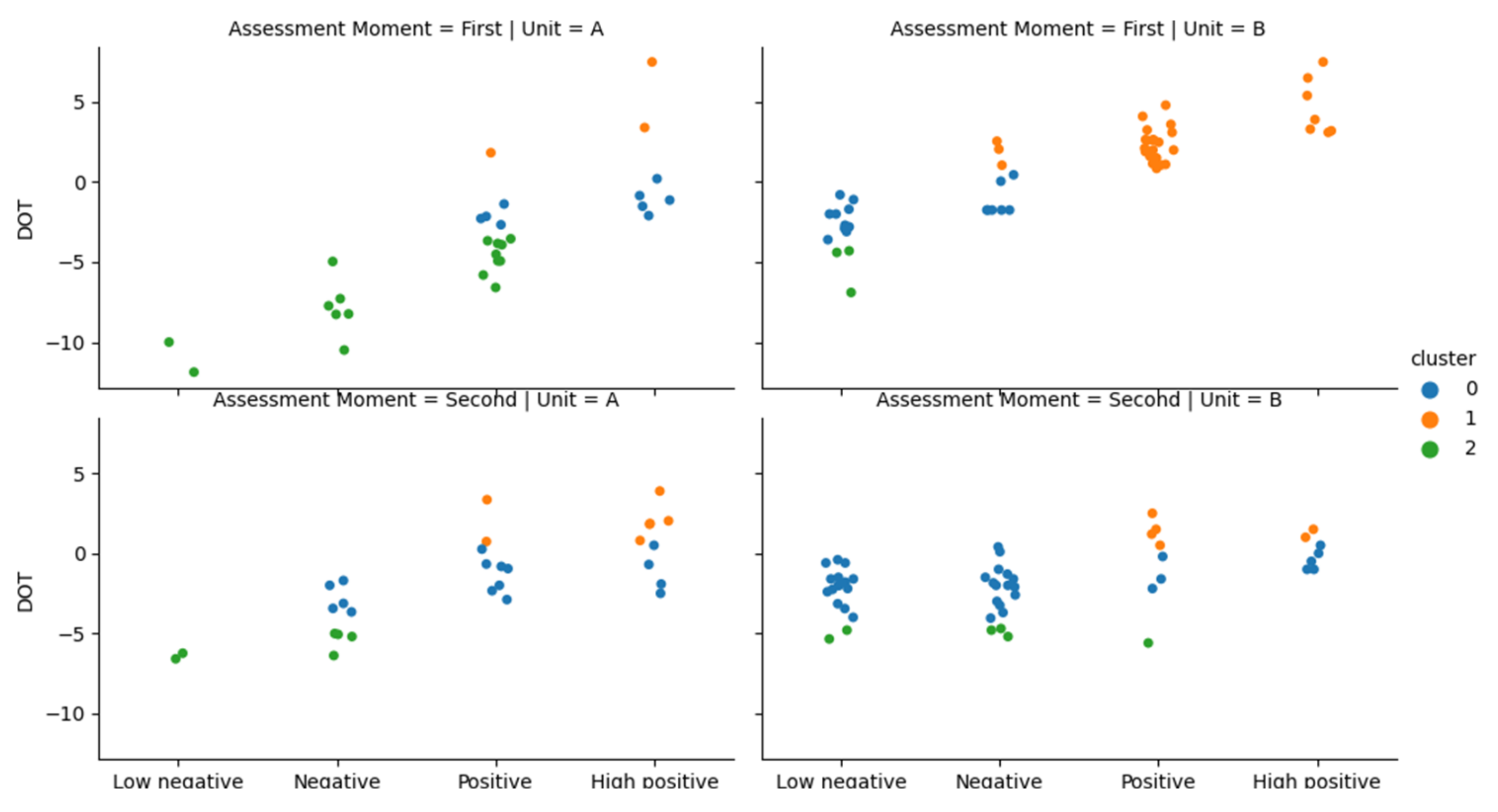
The second clustering was performed using the K-prototypes algorithm in Python, with K = 3. It was performed in a single dataset, containing four variables: the DOT, the grade level (low-negative (below 5 values: [0,5]), negative (between 5 and 10 values: [5,10[), positive (between 10 and 15 values: [10,15]), high-positive (over 15 values: [15,20]), the assessment moment (first, or second), and the unit (A, or B). Figure 8 presents the clusters found in this process.

In the figure the clusters are presented by unit, assessment moment, and grade level. The clustering basically grouped the elements by their DOT: cluster 0 groups the students who can almost accurately assess their work; cluster 1 groups the students who under-assess their work; and cluster 2 groups the students who over-assess their work. In the first assessment moment there are more over-assessing students in Unit A (cluster 2, in green in the figure) and more under-assessing students in Unit B (cluster 1, in orange in the figure). In the second assessment moment, most students are included in cluster 0 (in blue in the figure), meaning that their assessment is more accurate.

5. Discussion

In Unit A, there are no significant correlations between DOT and age nor gender, for both assessment moments (the p-value for age is 0.741 and, for gender, it is 0.649). There is, however, a correlation between the DOT and the grade obtained in the first moment of assessment.

In the first assessment moment, students graded in the low-negative range (with a grade lower than five values) predict, on average, a grade 10.94 higher than the grade obtained; students graded in the negative range (with grades between 5 and 10) predict, on average, a grade 7.83 values higher than the grade obtained; students graded in the positive range (with grades between 10 and 15) predict, on average, a grade 3.55 higher than the grade obtained; finally, students graded in the high-positive range (with a grade of 15 or higher) predict, on average, a grade 0.40 lower than the grade obtained.

In the second assessment moment there is still a correlation, but it is less pronounced: students graded in the low-negative range (with a grade lower than five values) predict, on average, a grade 2.06 higher than the grade obtained; students graded in the negative range (with grades between 5 and 10) predict, on average, a grade 2.65 values higher than the grade obtained; students graded in the positive range (with grades between 10 and 15) predict, on average, a grade 0.53 higher than the grade obtained; finally, students graded in the high-positive range (with a grade of 15 or higher) predict, on average, a grade 0.04 lower than the grade obtained. In this case, the p-value for the grades is 0.000, which indicates that the null hypothesis ($H_0$ = “The grades occurred randomly”) should be rejected, which suggests a strong correlation between grades and DOT.

In Unit B, there is a small correlation between DOT and age, with 18-year-old students predicting a slightly worse grade than those who are over 18 years old (p-value = 0.257). In Unit B, there is a small correlation between DOT and gender, with male students predicting a slightly worse grade than they did compared to female students (p-value = 0.472). As happened in Unit A, also in Unit B there is a high correlation between the DOT and the grades obtained by the students (p-value = 0.000).

In the first assessment moment, students graded in the low-negative range (with a grade lower than five values) predict, on average, a grade 2.95 higher than the grade obtained; students graded in the negative range (with grades between 5 and 10) predict, on average, a grade 0.26 values higher than the grade obtained; students graded in the positive range (with grades between 10 and 15) predict, on average, a grade 2.36 lower than the grade obtained; finally, students graded in the high-positive range (with a grade of 15 or higher) predict, on average, a grade 4.7 values lower than the grade obtained.

In the second assessment moment, students graded in the low-negative range (with a grade lower than five values) predict, on average, a grade 2.06 higher than the grade obtained; students graded in the negative range (with grades between 5 and 10) predict, on average, a grade 2.65 values higher than the grade obtained; students graded in the positive range (with grades between 10 and 15) predict, on average, a grade 0.53 higher than the grade obtained; finally, students graded in the high-positive range (with a grade of 15 or higher) predict, on average, a grade 0.40 lower than the grade obtained.

To improve the understanding of these results, and for easier visualization, the figure below (Figure 6), presents the DOT for the two evaluation moments and for the two courses. In the figure, the average DOT is presented for the first and second assessment moments of Unit A (1A and 1B, respectively) and also for the two assessment moments in Unit B (1B and 2B).

According to Figure 9, the DOT average in Unit A is higher than in Unit B, and this difference is more accentuated in the first assessment moment. This might occur due to Computer Science and Computer Engineering students being, traditionally, more pessimistic about their test results. It may also be related to the type of assessment: as mentioned previously, in Unit B, the assessment includes writing a program. Since the students can test their code, they often think that if it does not work correctly, the grade given to that item will be 0.

In both cases (Unit A and Unit B), it is verified that the students improved their self-assessment capacity from the first assessment moment to the second assessment moment. This is visible by the decrease in the DOTs averages and is most perceptive in Unit A: in the first assessment moment we have an average DOT of −3.85, while for the second assessment moment the DOT average is −1.65.

6. Conclusions

The benefits of involving students in the assessment process are described in the literature. In this way, it can be considered that students are part of the entire learning process—and actively—self-regulated learning. The problem that arises is whether students can self-assess themselves, whether the self-assessment process can be improved, and whether there are characteristics associated with students that are favorable for a more accurate self-assessment.

An experiment was carried out in two different curricular units and in the two assessment moments. Students were asked to self-assess their work, based on the teacher’s evaluation criteria and grid (which included the weights given to each criterium). The measure used was the DOT (difference between the grade obtained and self-assessed). Results indicate that DOT is proportional to the grades obtained—that is, the students’ level of knowledge (and probably work). In the second moment of evaluation the differences are smaller but still exist. The results suggest that the students with lower grades think they will get a grade much higher than they really deserve, while students with higher grades think they will get a grade slightly lower than the grade they deserve.

This experience brings two major conclusions: the students’ difficulty in self-assessment (even knowing the assessment criteria and their weights); and that the students’ ability to self-assess can be improved through time, with experience. Thus, it is very difficult and unfair to consider self-assessment as one of the evaluation criteria to be used for the final grade. It could lead to great injustices for students with greater knowledge.

Knowing that the self-assessment process is so important for student engagement, there is a need to make this process much more regular and habitual. In this way, students could become much more used to self-assessment, they would do it better and, consequently, the process would have a much more positive effect.

As a future work, we intend to implement a more regular self-assessment during the semester to verify if the disparities found in this study are attenuated. Besides, we plan to acquire more data (by encouraging students to complete the surveys), to overcome the problem of having a low number of eligible students for the study, as mentioned in Section 3.2.

References

1. Mayer, R. Should there be a three-strikes rule against pure discovery learning? The case for guided methods of instruction. Am. Psychol. 2004, 59, 14–19. [Google Scholar] [CrossRef] [PubMed] [Green Version]
2. Lea, S.J.; Stephenson, D.; Troy, J. Higher Education Students’ Attitudes to Student-centred Learning: Beyond ’educational bulimia’? Stud. High. Educ. 2003, 28, 321–334. [Google Scholar] [CrossRef]
3. Felder, R.M.; Brent, R. Navigating the Bumpy Road to Student-Centered Instruction. Coll. Teach. 1996, 44, 43–47. [Google Scholar] [CrossRef]
4. Agustini, K.; Wahyuni, D.S.; E Mertayasa, I.N.; Wedhanti, N.K.; Sukrawarpala, W. Student-centered learning models and learning outcomes: Meta-analysis and effect sizes on the students’ thesis. J. Physics Conf. Ser. 2021, 1810. [Google Scholar] [CrossRef]
5. Bonwell, C.C.; Eison, J.A. Active Learning: Creating Excitement in the Classroom; ASHE-ERIC Higher Education: Washington, DC, USA, 1991. [Google Scholar]
6. Zhang, L.; Basham, J.D.; Carter, R.A.; Zhang, J. Exploring Factors associated with the implementation of student-centered instructional practices in U.S. classroomss. Teach. Teach. Educ. 2021, 99, 103273. [Google Scholar] [CrossRef]
7. Zimmerman, B. Theories of Self-Regulated Learning and academic achievement: An overview and analysis. In Self-Regulated Learning and Academic Achievement: Theoretical Perspectives; Taylor & Francis: Abingdon, UK, 2008. [Google Scholar]
8. Zimmerman, B.J. Attaining self-regulation: A social cognitive perspective. In Handbook of Self-Regulation; Boekaerts, M., Pintrich, P.R., Zeidner, M., Eds.; Academic Press: Cambridge, MA, USA, 2000; pp. 13–40. [Google Scholar]
9. Pintrich, P.R. The Role of Goal Orientation in Self-Regulated Learning. In Handbook of Self-Regulation; Academic Press: Cambridge, MA, USA, 2000; pp. 451–502. [Google Scholar]
10. Urbina, S.; Villatoro, S.; Salinas, J. Self-Regulated Learning and Technology-Enhanced Learning Environments in Higher Education: A Scoping Review. Sustainability 2021, 13, 7281. [Google Scholar] [CrossRef]
11. Bandura, A. Social Foundations of Thought and Action: A Social Cognitive Theory; Prentice-Hall: Englewood Cliffs, NJ, USA, 1986. [Google Scholar]
12. Boekaerts, M. Self-regulated Learning at the Junction of Cognition and Motivation. Eur. Psychol. 1996, 1, 100–112. [Google Scholar] [CrossRef]
13. Winne, P.; Hadwin, A. Studying as self-regulated learning. In Metacognition in Educational Theory and Practice; Routledge: Abingdon, UK, 1998; pp. 291–318. [Google Scholar]
14. Tormey, R.; Hardebolle, C.; Pinto, F.; Jermann, P. Designing for impact: A conceptual framework for learning analytics as self-assessment tools. Assess. Evaluation High. Educ. 2019, 45, 901–911. [Google Scholar] [CrossRef]
15. Nocol, D.; Macfarlane, D. Formative Assessment and Self-Regulated Learning: A Model and Seven Principles of Good Feedback Practice. Stud. High. Educ. 2006, 31, 199–218. [Google Scholar] [CrossRef]
16. Nulty, D.D. Peer and self-assessment in the first year of university. Assess. Evaluation High. Educ. 2011, 36, 493–507. [Google Scholar] [CrossRef]
17. Pérez-Loredo, L. La Evaluación Dentro del Proceso Enseñanza-Aprendizaje. La Academia. Available online: https://ruidera.uclm.es/xmlui/bitstream/handle/10578/7951/La_evaluaci_n_del_proceso_de_ense_anza-aprendizaje.pdf (accessed on 27 September 2021).
18. Orsmond, P.; Merry, S.; Reiling, K. The Use of Student Derived Marking Criteria in Peer and Self-assessment. Assess. Evaluation High. Educ. 2000, 25, 23–38. [Google Scholar] [CrossRef]
19. Boud, D.; Dochy, F. Assessment 2020: Seven propositions for assessment reform in higher education; Australian Learning and Teaching Council: Sydney, NSW, Australia, 2010. [Google Scholar]
20. Tan, K.H. Qualitatively different ways of experiencing student self?assessment. High. Educ. Res. Dev. 2008, 27, 15–29. [Google Scholar] [CrossRef]
21. Mok, M.M.C.; Lung, C.L.; Cheng, D.P.W.; Cheung, H.P.R.; Ng, M.L. Self-assessment in higher education: Experience in using a metacognitive approach in five case studies. Assess. Evaluation High. Educ. 2006, 31, 415–433. [Google Scholar] [CrossRef]
22. Grimes, P.W. The Overconfident Principles of Economics Student: An Examination of a Metacognitive Skill. J. Econ. Educ. 2002, 33, 15–30. [Google Scholar] [CrossRef]
23. Savin-Baden, M. Understanding the impact of assessment on students in problem-based learning. Innov. Educ. Teach. Int. 2003, 221–233. [Google Scholar] [CrossRef]
24. Ribeiro, L.R.D.C.; Filho, E.E. Avaliação formativa no ensino superior: Um estudo de caso. Acta Sci. Hum. Soc. Sci. 2011, 33, 45–54. [Google Scholar] [CrossRef]
25. Adams, J.B. What Makes the Grade? Faculty and Student Perceptions. Teach. Psychol. 2005, 32, 21–24. [Google Scholar] [CrossRef]
26. Remedios, R.; Lieberman, D.A.; Benton, T.G. The effects of grades on course enjoyment: Did you get the grade you wanted? Br. J. Educ. Psychol. 2000, 70, 353–368. [Google Scholar] [CrossRef]
27. Olina, Z.; Sullivan, H.J. Student self-evaluation, teacher evaluation, and learner performance. Educ. Technol. Res. Dev. 2004, 52, 5–22. [Google Scholar] [CrossRef]
28. León, S.; Augusto-Landa, J.; García-Martínez, I. Moderating Factors in University Students’ Self-Evaluation for Sustainability. Sustainability 2021, 13, 4199. [Google Scholar] [CrossRef]
29. Sobral, S.R. CS1 Student Grade Prediction: Unconscious Optimism vs Insecurity? Int. J. Inf. Educ. Technol. 2021, 11, 387–391. [Google Scholar] [CrossRef]
30. Miller, T.M.; Geraci, L. Unskilled but aware: Reinterpreting overconfidence in low-performing students. J. Exp. Psychol. Learn. Mem. Cogn. 2011, 37, 502–506. [Google Scholar] [CrossRef] [Green Version]
31. Nunn, G. Adult learners’ locus of control, self-evaluation and learning temperament as a function of age and gender. J. Instr. Psychol. 1994, 21, 260–264. [Google Scholar]
32. Lundeberg, M.A.; Fox, P.W.; Punćcohaŕ, J. Highly confident but wrong: Gender differences and similarities in confidence judgments. J. Educ. Psychol. 1994, 86, 114–121. [Google Scholar] [CrossRef]
33. Landrum, R. Student Expectations of Grade Inflation. J. Res. Dev. Educ. 1999, 32, 124–128. [Google Scholar]
34. Svanum, S.; Bigatti, S. Grade Expectations: Informed or Uninformed Optimism, or Both? Teach. Psychol. 2006, 33, 14–18. [Google Scholar] [CrossRef]
35. Belski, R.; Belski, I. Can students predict their grade accurately in order to self-regulate? In Proceedings of the 24th Annual Conference of the Australasian Association for Engineering Education-AAEE2013, Gold Coast, QLD, Australia, 8–11 December 2013. [Google Scholar]
36. Thawabieh, A.M. A Comparison between Students’ Self-Assessment and Teachers’ Assessment. J. Curric. Teach. 2017, 6, 14. [Google Scholar] [CrossRef] [Green Version]
37. Winne, P.; Jamieson-Noel, D. Exploring students’ calibration of self reports about study tactics and achievement. Contemp. Educ. Psychol. 2002, 27, 551–572. [Google Scholar] [CrossRef]
38. Hacker, D.; Bol, L.; Bahbahani, K. Explaining calibration accuracy in classroom contexts: The effects of incentives, reflec-tion, and explanatory style. Metacognition Learn. 2008, 3, 101–121. [Google Scholar] [CrossRef]
39. Sullivan, K.; Hall, C. Introducing Students to Self-assessment. Assess. Eval. High. Educ. 1997, 22, 298–305. [Google Scholar] [CrossRef]
Figure 1. Evolution of the SSE with K in clustering with K-means.
Bdcc 05 00081 g001
Figure 2. Evolution of the clustering cost function with K in clustering with K-prototypes.
Bdcc 05 00081 g002
Figure 3. Histogram of the DOTs of students on both units, and in both assessment moments.
Bdcc 05 00081 g003
Figure 4. Visual representation of the clusters obtained when considering the first test of Unit A.
Bdcc 05 00081 g004
Figure 5. Visual representation of the clusters obtained when considering the second test of Unit A.
Bdcc 05 00081 g005
Figure 6. Visual representation of the clusters obtained when considering the first test of Unit B.
Bdcc 05 00081 g006
Figure 7. Visual representation of the clusters obtained when considering the second test of Unit B.
Bdcc 05 00081 g007
Figure 8. Cluster representation.
Bdcc 05 00081 g008
Figure 9. Average DOT for Units A and B, two assessment moments (1 and 2) by grade level.
Bdcc 05 00081 g009