Article

Automatic Diagnosis of Epileptic Seizures in EEG Signals Using Fractal Dimension Features and Convolutional Autoencoder Method

1
Department of Electrical Engineering, Gonabad Branch, Islamic Azad University, Gonabad 6518115743, Iran
2
Department of Electrical Engineering, Mashhad Branch, Islamic Azad University, Mashhad 9187147578, Iran
3
Institute for Intelligent Systems Research and Innovation (IISRI), Deakin University, Waurn Ponds, VIC 3216, Australia
*
Author to whom correspondence should be addressed.
Big Data Cogn. Comput. 2021, 5(4), 78; https://doi.org/10.3390/bdcc5040078
Submission received: 30 October 2021 / Revised: 3 December 2021 / Accepted: 8 December 2021 / Published: 13 December 2021

Abstract

:
This paper proposes a new method for epileptic seizure detection in electroencephalography (EEG) signals using nonlinear features based on fractal dimension (FD) and a deep learning (DL) model. Firstly, Bonn and Freiburg datasets were used to perform experiments. The Bonn dataset consists of binary and multi-class classification problems, and the Freiburg dataset consists of two-class EEG classification problems. In the preprocessing step, all datasets were prepossessed using a Butterworth band pass filter with 0.5–60 Hz cut-off frequency. Then, the EEG signals of the datasets were segmented into different time windows. In this section, dual-tree complex wavelet transform (DT-CWT) was used to decompose the EEG signals into the different sub-bands. In the following section, in order to feature extraction, various FD techniques were used, including Higuchi (HFD), Katz (KFD), Petrosian (PFD), Hurst exponent (HE), detrended fluctuation analysis (DFA), Sevcik, box counting (BC), multiresolution box-counting (MBC), Margaos-Sun (MSFD), multifractal DFA (MF-DFA), and recurrence quantification analysis (RQA). In the next step, the minimum redundancy maximum relevance (mRMR) technique was used for feature selection. Finally, the k-nearest neighbors (KNN), support vector machine (SVM), and convolutional autoencoder (CNN-AE) were used for the classification step. In the classification step, the K-fold cross-validation with k = 10 was employed to demonstrate the effectiveness of the classifier methods. The experiment results show that the proposed CNN-AE method achieved an accuracy of 99.736% and 99.176% for the Bonn and Freiburg datasets, respectively.

1. Introduction

Epilepsy is a neurological disorder that has threatened many lives [1,2]. If diagnosed late, the epileptic seizure will cause irreparable damages to the patient [1,2]. Generally, epileptic seizures are divided into three groups of general [3], focal [4], and epilepsy with unknown symptoms [5]. According to the World Health Organization (WHO), more than 60 million individuals suffer from different types of epileptic seizures, and their lives are threatened with severe health issues [6,7].
Neuroimaging modalities are among the essential techniques for epileptic seizure detection, including functional and structural techniques [8,9]. The analysis of the anatomy and anatomical connections of various parts of the brain is performed using structural neuroimaging modalities, such as structural magnetic resonance imaging (sMRI) and diffusion tensor imaging (DTI) [10]. On the other hand, by using functional neuroimaging modalities, specialists can investigate the activities and functional connectivity of the brain accurately [8]. EEG is the primary functional neuroimaging modality with utmost importance for epileptic seizure detection [11].
EEG signals provide specialist physicians with essential information regarding brain performance at the time of epileptic seizures [11,12,13]. Compared to other neuroimaging methods, this modality is relatively cost-effective and has suitable performance. On the other hand, EEG has different channels at the time of recording the brain, making its signals more complicated [5]. EEG signals have different artifacts at the time of recording, such as urban electricity, muscles, etc. These issues create some challenges for specialist physicians in the diagnosis of epileptic seizures using EEG signals [14].
The diagnosis of epileptic seizures using EEG signals is of significant importance to specialist physicians. Nowadays, a wide range of research is being conducted on the implementation of computer-aided diagnosis system (CADS) based on artificial intelligence (AI) in neurological disorders [15,16,17,18], especially epileptic seizures detection [19,20,21,22]. The CADS based on AI consists of preprocessing, feature extraction, feature selection, and classification steps [19,20,21]. Feature extraction is the essential step of CADS in epileptic seizure detection using EEG signals [7]. The feature extraction techniques from EEG signals consists of time [22], frequency [23], time-frequency [24], and nonlinear [25] fields. EEG signals have chaotic features, which has led researchers to employ different feature extraction methods in studies on epileptic seizure detection, such as entropies [26], largest Lyapunov exponent (LLE) [27,28], FDs techniques, etc.
In this paper, nonlinear feature extraction techniques based on FDs are employed in the epileptic seizure detection. 
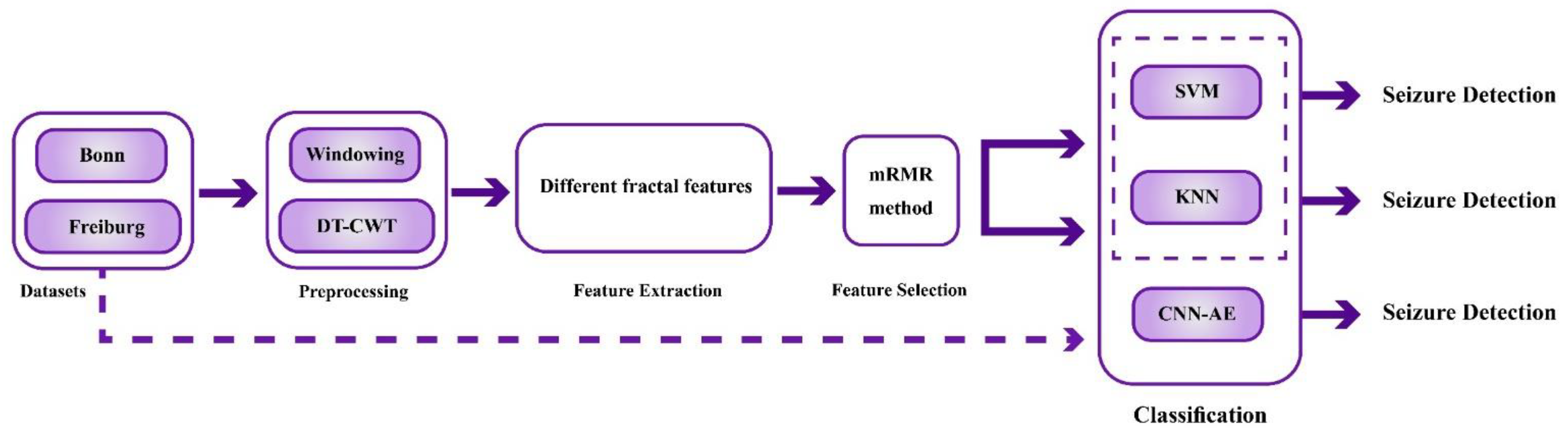
Figure 1 shows the block diagram of the proposed method for epileptic seizure detection. The Bonn [29] and Freiburg [30] datasets are employed to perform experiments. In the preprocessing step, all datasets are prepossessed using a Butterworth band pass filter with 0.5–60 Hz cut-off frequency. Following this, the EEG signals of both datasets are segmented into various time windows. Afterward, decomposition of the EEG signals into different sub-bands is carried out using DT-CWT [31,32].
The DT-CWT was first proposed by Kingsbury [33]. The DT-CWT has two parallel structures for obtaining real and imaginary parts of EEG signals. As compared to DWT, DT-CWT has several advantages, such as approximate shift immutability [34,35]. This helps to extract meaningful frequency information from each EEG signal [36]. The DT-CWT conversion is used in this paper with five decomposition levels, and a variety of fractal-based features are extracted from each decomposition level.
In the feature extraction step, various nonlinear features based on FDs are extracted from DT-CWT sub-bands, including HE [37], PFD [38], KFD [38], HFD [38], BC [39], MBC [39], Sevcik [40], DFA [41], RQA [42], MSFD [43], and MF-DFA [44]. FD features contain crucial information about EEG signals, and for this purpose they were used in the present study [45]. This research is the first to combine these feature extraction methods, highlighting the significance of this article.
In the feature selection step, the mRMR method [46] is employed. In this section, the proposed method selected 25 features. Ultimately, the KNN [47], SVM [48,49], and CNN-AE methods are employed for classification. The CNN-AE classifier method with a proposed number of layers is used for the first time in this paper.
Other sections of the article are presented as follows: Section 2 explores previous research carried out on epileptic seizure detection using the FD techniques. The proposed method for epileptic seizure detection is presented in Section 3. The experiment results are presented in Section 4. Section 5 presents statistical parameters for classification performance. Then, the discussion is presented in Section 6. Finally, conclusions and future works are presented in Section 7.

2. Related Works

This section presents a literature review of previous investigations into the diagnosis of epileptic seizures via EEG signals and FD feature extraction techniques. The first study by Wijayanto et al. [50] proposed an automated epileptic seizure detection based on the FD theory. First, the EEG signals were decomposed into five sub-bands. Afterward, the KFD was employed for feature extraction. Ultimately, the SVM method was employed for the classification of features. The results of the research showed that they could obtain favorable results.
El-Kishky et al. [51] employed different features for epileptic seizure detection. In this research, the EEG signals were first preprocessed. Afterward, various features, including HE, HFD, and Shannon entropy, were extracted from the EEG signals.
In another study, Jacob et al. [52] employed discrete wavelet transform (DWT) in the preprocessing step. Then, KFD and HFD features were extracted from DWT sub-bands. Finally, the SVM classifier was employed for classification.
Yuan et al. [51] proposed an intelligent method of epileptic seizure detection using EEG signals. In their proposed method, different techniques were employed in the preprocessing step. Afterward, differential box-counting (DBC) was investigated for feature extraction in EEG signals. They employed the SLFN method in the classification step and obtained favorable results.
In [52], the proposed method of epileptic seizure detection is implemented on the Freiburg dataset. In this study, the noises of the EEG signals were eliminated and then decomposed into time periods. Afterward, the FDs and gradient boosting methods were employed in the feature extraction, and classification steps, respectively.
Yang et al. [53] employed a new feature extraction method based on the FD theory for diagnosis of epileptic seizures using EEG signals. The dataset they employed for carrying out the experiments was of clinical type. The GFD feature extraction method was employed in this study. Following this, the run covering and SVM methods were employed in the feature selection and classification steps, respectively.
Moctezuma et al. [54] employed the CHB-MIT dataset to implement their proposed epileptic seizure diagnosis method. In this research, decomposition and preprocessing of EEG signals into different sub-bands was carried out using the empirical mode decomposition (EMD) method. Next, energy distribution and FD features were extracted from each EMD sub-band. Following this, K-means clustering and SVM methods were employed in the feature selection and classification steps, respectively.
In [55], an epileptic seizure diagnosis method via EEG signals based on the GFD technique was proposed. The Bonn dataset was employed to carry out experiments. In this research, the noises of the EEG signals were first eliminated in the preprocessing step and then decomposed into different sub-bands using DWT. The GFD method and the Renyi entropy were extracted from DWT sub-bands in the feature extraction step. Following this, the analysis of variance (ANOVA) test with the box plot method was employed in the feature selection method.
In [56], a method of epileptic seizure diagnosis using different FD methods was proposed. Different methods such as noise elimination, windowing of signals, and finally decomposition of EEG signals into different sub-bands were implemented in the preprocessing step. Next, the HFD, KFD, and Sevcik features were extracted from DWT sub-bands. Finally, the SVM was used for classification.
Sikdar et al. [57] employed the DWT to analyze the EEG signals of the Bonn dataset into different sub-bands. They investigated the MFDFA method for feature extraction. Finally, the statistical analysis and SVM methods were employed in the feature selection and classification steps, respectively.
Dalal et al. [58] used the FAWT method in the preprocessing step of the EEG signals. Then, they used the HFD and Kruskal–Wallis statistical test methods in the feature extraction and feature selection steps. Then, the SVM method was employed in the classification step.
This section introduced several articles on the diagnosis of epileptic seizures via EEG signals using the fractal technique. Other articles are introduced in Table 1.

3. Material and Methods

In this section, the steps of the proposed method are presented. First, the EEG dataset for epileptic seizures detection is introduced. In the second step, the preprocessing of EEG signals is conducted according to the DT-CWT method. In the third step, various feature extraction techniques based on FD are introduced. The fourth step is pertinent to the feature selection technique. Finally, various types of classifier algorithms are presented in step five.

3.1. Dataset

3.1.1. The Bonn Dataset

The Bonn dataset consists of five sets of D, C, B, A, and E, and each one includes 100 single-channel signals with a time duration of 23.6 s [29]. All EEG signals from this dataset are recorded in the form of 12-bit with a sampling frequency of 173.61 Hz. In this dataset, the A and B sets of the EEG signals of five individuals are normal, where the A set of EEG signals is pertinent to the case of eyes open and the B set is pertinent to the case of eyes closed. The C and D sets include the EEG signals of five patients at the pre-ictal time [24]. Ultimately, the E set includes the seizure time of five patients with epilepsy with ictal time. In this dataset, the EEG signals of the A and B sets are recorded from the scalp, and the D, C, and E sets are recorded in an invasive way. Invasive electrodes are inserted into the hippocampal formation site symmetrically. All EEG signals are recorded by a 128-channel amplifier using a common, normal reference [29]. Further information regarding the dataset is presented in Table 2 and Table 3. In addition, Figure 2 shows a sample of five sets of the Bonn dataset.

3.1.2. The Freiburg Dataset

In this dataset, the Intracranial EEG (IEEG) signals were recorded in the Freiburg hospital, Germany, from 21 patients with focal epilepsy [30]. All IEEG signals from this dataset are recorded with a sampling frequency of 256 Hz and strip, depth, and grid electrodes [25]. The age range of the patients in this dataset was between 10 and 50 years, and thirteen individuals were female, and eight individuals were male. In this dataset, there are different pre-ictal, ictal, and inter-ictal times of patients with epileptic seizures. Three different types of seizures are reported among the patients, including complex partial (CP), generalized tonic-clonic (GTC), and simple partial (SP) [30]. Each one of the patients has experienced at least two types of these seizures. Further details regarding this dataset are provided in Table 4 [30]. Figure 3 shows a section of the EEG signals from the Freiburg dataset.

3.2. Preprocessing

This DT-CWT was first proposed by Kingsbury [33] and then improved by Ivan [34,35,36], in which two wavelet filter trees are used to obtain the wavelet coefficients corresponding to the real and imaginary parts of the wavelet [33]. Figure 4 shows the DT-CWT structural. As shown in Figure 4, h 0 and h 1 show low and high-pass filters for real coefficients. Furthermore, g 0 and g 1 represent low and high-pass filters for imaginary coefficients. In addition, (↓2) indicates a decrease in the sampling rate [33].
Here, the first and second filter banks are represented by symbols ψ ( t ) and ψ ( t ) , respectively, and the complex wavelet base is defined as (1) [33]:
Ψ t ( t ) = ψ ( t ) + ψ ( t ) .
The filter bank ψ ( t ) is defined as follows [33]:
ψ ( t ) = 2 n h 1 ( n ) ( 2 t n ) .
where
( t ) = 2 n h 0 ( n ) ( 2 t n ) .
Equations are ψ ( t ) also similar to Equations (1) and (2), where parameters h 1 and h 0 are substituted with g 1 and g 0 , respectively. Ideally, ψ ( t ) is equal to Hilbert transform ψ ( t ) as follows [33]:
ψ ( t ) = H { φ ( t ) } .
An important step in establishing Equation (4) is that g 0 is equal to half the delayed sample of h 0 ( n ) [33].
g 0 ( n ) h 0 ( n 0 · 5 ) .  
In addition, in the case of orthogonal wavelet, Equation (4) is satisfied if [33]:
H 0 ( e j w ) = e j 0.5 ω H 0 ( e j ω ) ,           f o r   | ω | < π .
Therefore, ideally, high-pass filters are defined as follows [33]:
H 1 ( e j w ) = j s g n ( ω ) e j 0.5 ω H 1 ( e j ω ) ,           f o r   | ω | < π .
For accurate DT-CWT running, the first step of the filter bank entails particular precision, otherwise frequency responses will not be accurately analyzed. Suppose the k t h step of the first filter bank that terminates with H 1 ( e j w ) . If H ( k ) ( e j w ) is the equivalent response, then we can apply new identities for k > 1, as represented as follows [33]:
H k ( e j ω ) = H 1 ( e j 2 k 1 ω ) m = 0 k 2 H 0 ( e j 2 m ω ) ,           f o r   | ω | < π .
If the equivalent response of the second filter bank of the corresponding branch, which is obtained by substituting H i with H i , is shown with H ( k ) ( e j w ) , then we have [33]:
H 1 ( e j ω ) = H 1 ( e j ω ) .
H ( 1 ) ( e j ω ) = H 1 ( e j ω ) .
Assuming pairs { h 0 , h 1 } ,   { g 0 ,   g 1 } satisfy Equations (6) and (7), it follows that for all k ≥ 1, H ( k ) ( e j w )   and H ( k ) ( e j w ) estimate the following equation [33]:
H ( k ) ( e j ω ) = j   s g n ( ω ) e j 0.5 ω H k ( e j ω ) ,           f o r   | ω | < π .
That is equal to [33]:
H ( k ) ( e j ω ) H ( k ) ( e j ω ) = H 0 ( e j ω ) H 0 ( e j w ) H ( k 1 ) ( e j 2 ω ) H ( k 1 ) ( e j 2 ω ) = j s g n ( ω ) e j 0.5 ω ,           f o r   | ω | < π .
Furthermore, if the k t h response of the new step of the first and second filter banks are shown with H n e w ( k ) ( e j w ) and H n e w ( k ) ( e j w ) , respectively, then we can conclude:
We have pairs of { h 0 , h 1 } ,   { g 0 ,   g 1 } which satisfy Equations (6) and (7) for k > 1 [33]:
H n e w ( k ) ( e j w ) = H { H n e w ( k ) ( e j w ) } .
If and only if [33]:
g 0 ( n ) = h 0 ( n 1 ) .
More information regarding DT-CWT is presented in [33]. In this study, we employed the Kingsbury toolbox, which covers various filters including Antonini (An), Q-shift (QS), LeGall (LeG), and near-symmetric (NS) filters [33]. Reference [
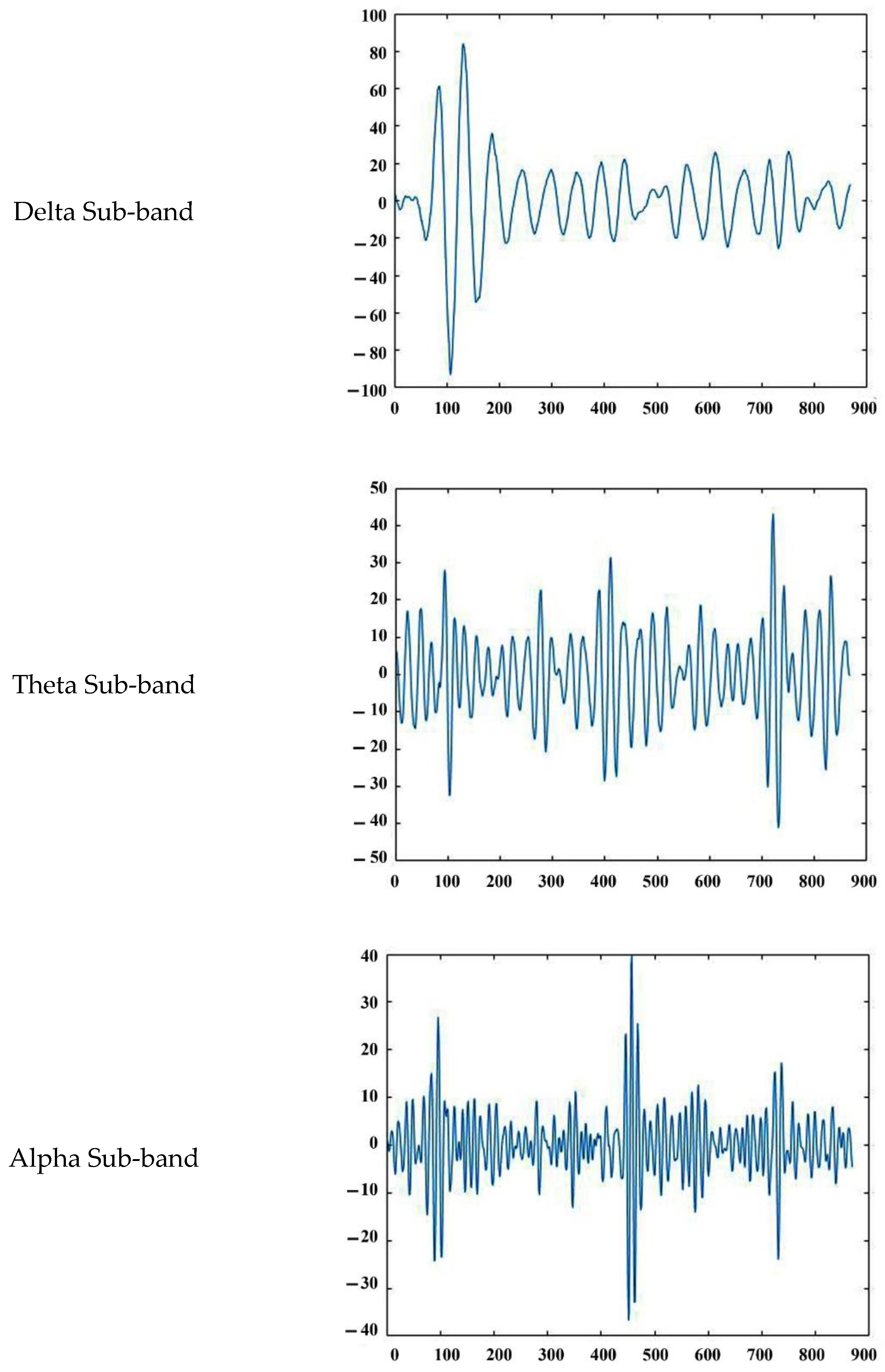
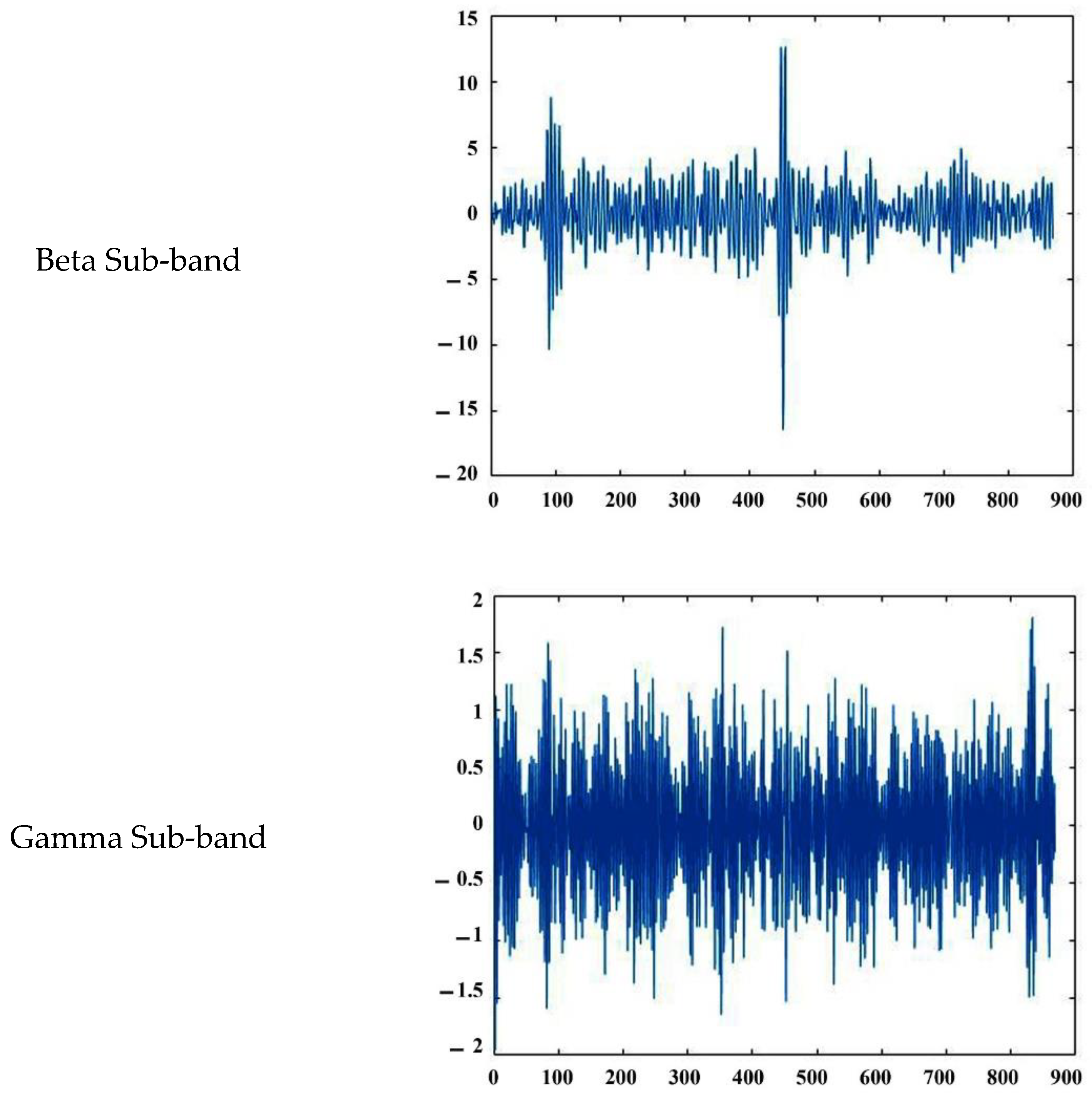
70] shows that NS 13/19 and QS 14/14 filters give more successful results than other filters. Therefore, we performed our simulations using these filters. We considered five sub-bands because of the five important cerebral frequencies for epileptic seizures detection, including delta, theta, alpha, beta, and gamma waves. Therefore, each EEG signal in the datasets were segmented into five sub-bands, and then FDs features were extracted from each sub-band. Figure 5 shows the five frequency sub-bands of an EEG signal using DT-CWT with NS 13/19 and QS 14/14 filters.

3.3. Feature Extraction

Feature extraction is accounted for as the essential step of epileptic seizure diagnosis. Various nonlinear features are introduced in this section. These features are mostly based on the FD theories.

3.3.1. Hurst Exponent

The HE is employed to calculate the correlation in time series, including EEG signals [37]. HE is widely used to assess whether there is a long-term correlation in a time series. According to the interesting features of HE, it is employed for feature extraction from EEG signals [37]. The HE relationship can be expressed as follows [37]:
  H E = log ( R S ) ( T ) .
where R is the difference between the maximum and minimum deviation and is pertinent to the mean. S indicates the standard deviation of the time series and T indicates the time duration of data [37].

3.3.2. Higuchi

The FD refers to the fractional or non-integer dimension of a geometric object. This dimension is a relative criterion of the number of structural blocks forming a pattern [38]. This feature is useful in different fields of the medical sciences [38]. Consider the x ( 1 ) , ( 2 ) , , N time series. Consider x m k Equation that expresses k number of time series:
x m k = { x ( m ) . x ( m + k ) . x ( m + 2 k ) x ( m + N m k k ) } ,               f o r     m = 1.2 k .
In the above equation, m is the initial time, k is a delay, and a is the integer part of a. Mean duration of L m ( k ) for each time series is defined as follows [38]:
L m ( k ) = i = 1 N m k | x ( m + i k ) x ( m + ( i 1 ) k ) | ( n 1 ) N m k k .
In the above equation, N and ( n 1 ) N m k k are the duration of time series x and normalization factor, respectively. In Equation (18), the sum of mean durations L (k) for each k display is indicated [38].
L ( k ) = m = 1 k L m ( k ) .

3.3.3. Katz

KFD is one of the FD techniques. In the KFD algorithm, the FD is calculated according to Equation (19) [38].
D = l o g 10 ( L ) l o g 10 ( d ) .
where L Is the length of the whole curve or the sum of distances between consecutive points in the time series, and d is the estimated diameter that is equal to the distance between the first point of the sequence and a point in the sequence. Mathematically, L and d are calculated as follows [38]:
d = max 2 i N { | x ( i + 1 ) x ( i ) | } .
L = i = 1 N 1 | x ( i + 1 ) x ( i ) | .
where i will be equal to the point with a maximum distance from 1 . The FD calculated by this method depends on the measurement unit. If the measurement unit changes, the calculated FD will change as well. The KFD method solved this problem using a general unit. L and d are normalized using the mean distance between consecutive points of a _ . Therefore, Equation (19) can be expressed as follows [38]:
D = l o g 10 ( L a _ ) l o g 10 ( d a _ ) .
The final Kartz equation can be expressed as follows by considering n = L a _ [38]:
D = l o g 10 ( n ) l o g 10 ( d L ) + l o g 10 ( n ) .

3.3.4. Petrosian

PFD is a quick method of estimating FD [38]. The PFD method is expressed as Equation (24) [38]:
D = l o g 10 n l o g 10 n + l o g 10 ( n n + 0.4 N Δ ) .
where n is the length of the sequence and N Δ is the number of changes in generated binary sequence [38].

3.3.5. Sevcik

The Sevcik algorithm is based on the Hausdorff dimension D h , defined as follows [39,40]:
D h = l i m ϵ 0 log N ( ε ) log ( ε ) .
In the equation above, N ( ε ) is the number of balls with ε radius. By defining N ( ε ) = 1 2 ε , the equation is written as follows [39,40]:
D h = l i m ϵ 0 log ( L ) log ( 2 ε ) log ( ε ) .
D h = l i m ϵ 0 1 log ( L ) log ( 2 ) log ( ε ) .
In this method, the signals are normalized in two dimensions, which is 1 square meter. The normalized value of x * and ordinate y * are as follows [39,40]:
x i * = x i x m a x .                                 i = 1 , 2 , , N
y i * = y i y m i n y m a x y m i n .                       i = 1 , 2 , , N
The square unit can be imagined as a network of N*N cells. The final equation is indicated in Equation (30) [39,40].
D s = l i m N ´ 0 1 + log ( L ) log ( 2 ) log ( 2 ( 1 N ) ) .

3.3.6. Box Counting

The BC method is one of the most important fractal methods, playing a crucial part in medical signals analysis [39]. In this method, the EEG signals are covered with a number of boxes, and their number is counted with a specific size to check how many are required for complete coverage. The mathematical definition is provided as follows [39]:
D B = l i m r 0 ( log N ( r ) / log ( 1 r ) ) .
In this equation, N ( r ) is the number of total boxes with r size. The counting box algorithm estimates the curve by the number of boxes required to cover the multiple box curve [39]. Thus,
log N ( r ) = D B log ( 1 r ) + c .
where C is a constant, the lowest square of the best straight line is considered as the DB box-counting dimension estimation of the curve [39].

3.3.7. Multiresolution Box-Counting

Assume a discrete-time signal s = { s ( 1 ) , s ( 2 ) , , s ( N ) } with the sampling frequency of f s with N samples. Each sample point s(i) is in the form of i = 1,…, N(X(i), y(i)). The steps of this method are defined in the following [39].
Step 1:
Consider two S(i) and S(i + 1) points indicating EEG signals with the interval of d t = x ( i + 1 ) x ( i ) = 1 f s , whose points height is in the form of h = y ( i + 1 ) y ( i ) . This method is repeated for all points on the EEG signal. In Equation (33), the total number of required boxes are provided to cover EEG signal with r resolution [39].
B ( r ) = s u m ( b ( i ) ) .     i = 1 , , N 1
Step 2:
Each intermittent point is placed on the signal to obtain the temporal resolution of r = 2 f s . It is repeated in this temporal resolution, and the total number of required boxes is calculated to cover the entire curve [39].
Step 3:
We receive the number of boxes to cover the curve by repeating the steps above for multiple temporal resolutions. For r = 1 f s   ,   2   f s   ,   ,   R f s that R f s the maximum temporal resolution is true where the investigated curve is placed [39].
Step 4:
The linear regression coefficient of curve log ( B ( r ) )   versus log ( 1 r )   is considered an EEG signal fractal dimension estimation [39].

3.3.8. DFA

In order to extract DFA, the method proposed by Peng et al. is employed [41]. Consider { x ( i ) ,   i = 1 , 2 , , N } time series. { y ( k ) } Time series can be obtained according to Equation (34) using the difference sum of {x(i)} time series from its mean [41].
  y ( k ) = i = 0 k [ x ( i ) x ] .
In this equation, <x> is the mean of {x(i)} time series [41].
In the next step, the obtained { y ( k ) } time series is divided into N n = i n t ( N / n ) identical windows with the length of n, and each window is a line on the point sets and is picked using the least square error method. Afterward, mean squared error function F ( n ) for whole time series { y ( k ) } and window length n is obtained according to Equation (35) [41].
F ( n ) = 1 N k = 1 N [ y ( k ) y n ( k ) ] 2 .  
In this equation, y n ( k ) is the time series obtained from the line in each window [41].

3.3.9. Recurrent Quantitative Analysis

Using these recurrent maps provides the possibility of not only reviewing but also quantifying the hidden pattern and finding structural changes and the similarities among various patterns in data [42]. Known as RQA, this ability is a nonlinear method of processing time series, capable of quantifying the repeat number and range in a dynamic system, thus, creating its trajectory in the phase space [42]. This method’s various criteria are provided in the following [42].
(1) Recurrent Rate
Recurrent Rate (RR) specifies the percentage of recurrent points in a map pertinent to the total correlation defined as follows [42]:
R R = 1 N 2 i , j = 1 N R i , j .
(2) DET
It defines the percentage of existing recurrent points of diagonal lines to the total recurrent points. The diagonal lines consist of two or multiple points that are neighbors in the diagonal form without any other distance [42].
D E T = l = l m i n N l P ( l ) i , j = 1 N R i , j .
(3) Lmax Index
It defines the biggest diagonal line length [42].
L m a x = m a x ( { l i ; i = 1 , , N l } ) .
(4) ENTR Index
It defines the entropy of diagonal lines [42].
E N T R = l = l m i n N P ( l ) l n ( P ( l ) ) .
(5) LAM Index
It defines the percentage of recurrent points creating the perpendicular (vertical) lines [42].
L A M = v = v m i n N v P ( v ) v = 1 N v P ( v ) .
(6) Trap Time (TT)
It defines the average length of vertical points [42].
T T = v = v m i n N v P ( v ) v = v m i n N P ( v ) .

3.3.10. Margaos-Sun Fractal Dimension (MSFD)

The MSFD is one of the other fractal methods used for extracting the features from signals or time series [43]. Similar to the aforementioned fractal methods, this method is of paramount importance in multi-dimensional signals analysis. In this method, the EEG signals of both datasets are segmented with different time length windows, and afterward, MSFD is applied to them. Further explanations regarding this method are provided in [43].

3.3.11. MFDFA

In this section, the MFDFA algorithm for the time series x k signal of length N is presented. This technique consists of five steps, which are described below [44].
In the first step, the cumulative deviation relation x k for   y ( i ) is calculated using the Equation (42) [44].
Y ( i ) = k = 1 i [ x k x ] .               ,   i = 1 , , N .
where
x = 1 N k = 1 N x k .
In Equation (43), the signal x k converts to the time series y ( i ) [44].
In the second step, y(i) is divided into Ns non-overlapping segments whose length is equal to s (Ns ≡ int (N/s)) [44].
In the third step, the least-squares for the polynomial series of order m are used to calculate distances v (v = 1,2,…, Ns) [44].
F 2 ( s , v ) = 1 s i = 1 s { Y [ ( v 1 ) s + i ] y v ( i ) } 2 .
For each segment v, v = 1,…, Ns and
F 2 ( s , v ) = 1 s i = 1 s { Y [ N ( v N s ) s + i ] y v ( i ) } 2 .
The effects of noise interference as well as non-static processes are eliminated at this stage. This leads to obtaining multi-fractal properties [44].
In the fourth step, the oscillation function of order qth is calculated for each scale s. This function has a qth RMS order [44].
F q ( s ) = { 1 2 N s v = 1 2 N s [ F 2 ( s , v ) ] q / 2 } 1 / q .
Finally, the comparison powers of the log-log diagrams of Fq (s) are calculated for each q in the fifth step. The relation of this section is defined as follows [44]:
F q ( s ) S h ( q ) .
In this relation, h(q) is generalized Hurst power. The generalized HE is as follows [44]:
τ ( q ) q h ( q ) 1 .
Note that a multi-fractal signal has multiple HEs. Moreover, the parameter τ(q) has a nonlinear relation with q [44].
In addition, it is proved that the singularity spectrum f (α) is related to h (q), which is shown in Equations (49) and (50).
α = h ( q ) + q h ( q ) .
f ( α ) = q [ α h ( q ) ] + 1 .
The spectrum can be specified using a quadratic function with minimum squares. It is important to note that the quadratic function in question must lie in the vicinity of α0.
f ( α ) = A ( α α 0 ) 2 + B ( α α 0 ) + C .
In this relation, C is an additive constant, and B is a measure of spectral asymmetry. Finally, the spectrum width is defined as follows [44]:
W = α 1 α 2 .
w i t h   f ( α 1 ) = f ( α 1 ) = 0 .
As indicated by width W, the spectrum in this relation is multi-fractal [44].

3.4. Information on Number of Features

This section describes the output values for each feature extraction technique. As discussed earlier, the DT-CWT technique was employed to decompose EEG signals into five sub-bands alpha, beta, gamma, theta, and delta. Then, a total number of 11 features were extracted from each DT-CWT sub-band, including MFDFA, MSFD, MBC, BC, Sevcik, DFA, HE, PFD, KFD, HFD, and RQA, each with its own output values. Additionally, some features had only one output and others possessed multiple outputs. The MSFD, Sevcik, DFA, HE, PFD, KFD, HFD, BC, and MRBC have a single output and MFDFA and RQA have multi outputs. The RQA method has six outputs and the MFDFA has different outputs. For the Bonn dataset with time windows of 5 s, the MFDFA has 51 outputs. Additionally, the MFDFA has 55 outputs for the Freiburg dataset with time windows of 4 s.
For the Bonn dataset, each EEG signal was segmented into time windows of 5 s. Time windows of 5 s have given the greatest accuracy in epileptic seizure detection according to [71]. For the Bonn dataset, the number of segments is equal to 2000, and 330 features (11 FDs) were extracted from each frame. As reported in [51], each EEG signal in the Freiburg dataset was segmented into time windows of 4 s. The number of features extracted for each frame of the Freiburg dataset was 350. Table 4 shows that the Freiburg dataset includes multiple subjects with various data lengths.

3.5. Feature Selection Using mRMR Method

mRMR is a feature selection method proposed by Peng et al. [46]. This method selects a group of features whose mutual information is minimal and with the output (class label) as the maximum value [46]. The mutual information of two features, x, and y, is defined as Equation (53), where p(x), p(y), and p(x, y) are the probability density functions (PDF) [46].
I ( x ; y ) =   p ( x , y ) log p ( x , y ) p ( x ) p ( y ) d x d y .
The maximum correlation or dependence between the features and class label is calculated via the formula as follows [46]:
max D ( S , c ) , D = 1 | S | x i ϵ S I ( x i ; c ) .
where S is the set of features and c is the class label. In addition, the minimum redundancy among the features is calculated via the formula as follows [46]:
min R ( S ) , R = 1 | S | 2 x i , X j S I ( x i , x j ) .
In the end, the mRMR equation is calculated as follows [46]:
max ( D , R ) , = D R .

3.6. Classification Methods

The proposed classification algorithms are examined in this section. In this study, the proposed classification methods include KNN [47], SVM [48,49], and the CNN-AE method. The novelty of this section is to employ the CNN-AE method with the number of proposed layers. An explanation of each method is provided in the following section.

3.6.1. Support Vector Machine

The SVM method is one of the well-established, popular, and best classification methods [48,49]. This method is widely used in various 2-class and multiclass classification problems with significantly high performance. In the SVM method, the 2-class or multiclass classification is performed using various kernels such as linear and RBF [48,49]. In this article, the RBF kernel is used to classify binary- and multiclass problems.

3.6.2. KNN

The KNN method, also used as a classification method, operates such that it finds the nearest neighbor for each data (according to the Euclidean distance) [47]. Afterward, it selects the K-nearest neighbor, specifying the data label based on the label of the majority. This method operates significantly slowly. More information on this method is provided in [47]. In this article, K is considered to be three.

3.6.3. Convolutional Autoencoder (CNN-AE)

Nowadays, DL methods have a special role in various medical applications, and numerous investigations are being conducted in this field [72,73,74,75]. Various DL models have been provided so far, the combined CNN-AE architecture is among them. Unsupervised learning-based CNN-AE is used for input data training [76,77]. This architecture has two parts, decoder and encoder, each of which uses convolutional layers [76,77]. In this method, first, data are entered into encoder layers, received in the output data in compressed form. Then, the encoder section data is received in the decoder section, and the data recovery operation is performed. In this study, a CNN-AE model together with the number of proposed layers is employed. The proposed method is shown in detail in Table 5.
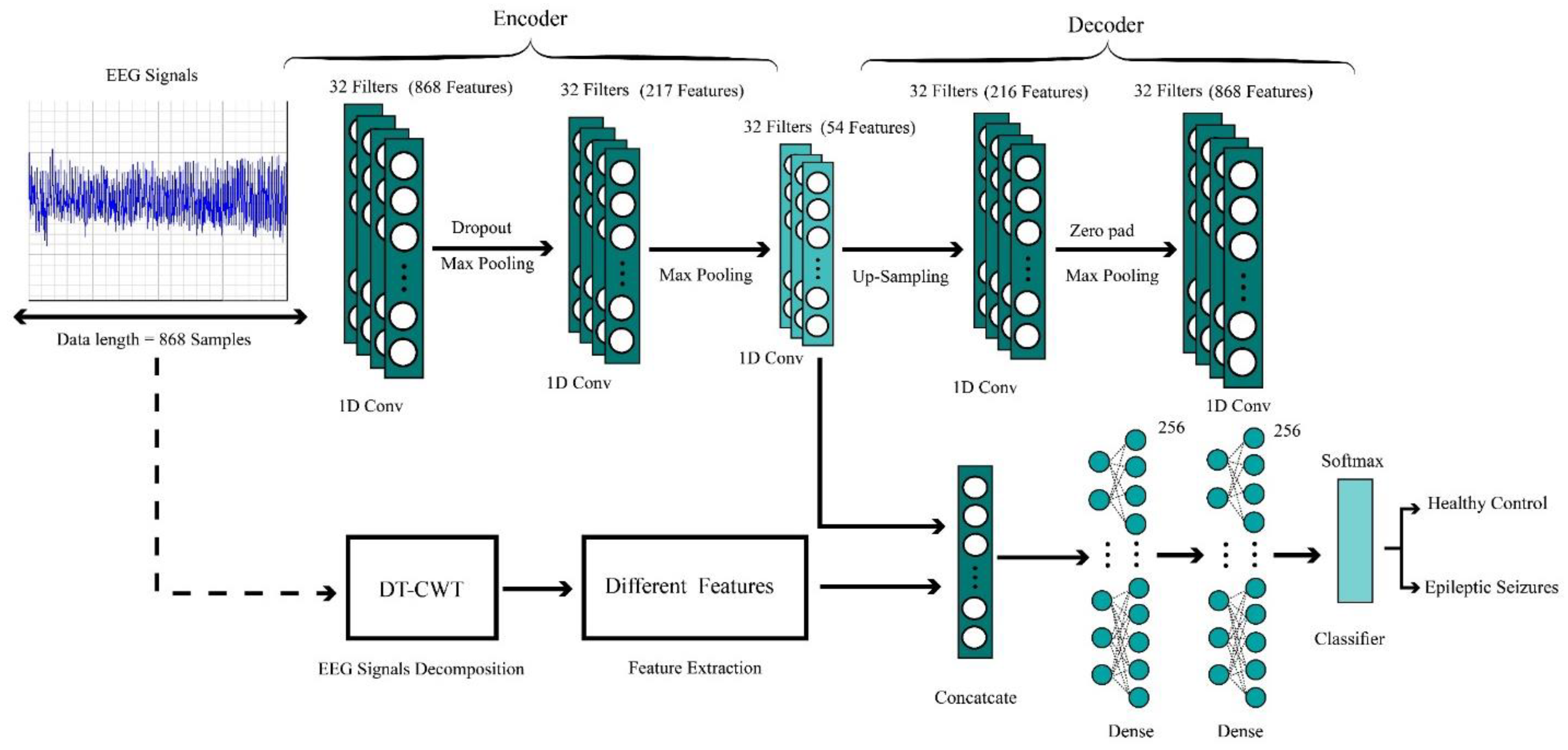
A block diagram of the proposed technique is shown in Figure 6, where the parameters of each layer in the Bonn dataset are illustrated for more simplicity. EEG signals of each dataset are first applied to the network’s inputs. As shown in Figure 6, EEG signals pass through the encoder layers allowing them to extract the features of interest. The input EEG signals are reconstructed in decoder layers. The number of features extracted are presented in Figure 6 and Table 5. As illustrated in Figure 6, handcrafted features are merged with features of the CNN-AE model upon feature reduction via mRMR. Here, 25 handcrafted features are merged with features of the CNN-AE model within the concatenate block. Thereupon, data were classified into three fully connected (FC) layers, with the first two layers having 256 neurons and the third layer incorporating the Softmax activation function. The steps used to extract features and classify data for the Freiburg dataset are similar to those used on the Bonn dataset.

4. Statistical Parameters for Classification Performance

The assessment parameters have a crucial role in demonstrating the performance of classification algorithms. In this paper, accuracy (Acc), precision (Prec), specificity (Spec), sensitivity (Sens), and F1_score statistical metrics are used [71]. The pertinent equations of each have been illustrated below. In addition, the K-fold cross validation with k = 10 is used for evaluation [71].
A c c = T P + T N F P + F N + T P + T N
S e n s = T P F N + T P .
S p e c = T N F P + T N .
F S = 2   T P 2   T P + F P + F N .

5. Experiment Results

In this section, we present the results of the proposed method. Simulations were performed using a hardware system with 16 GB RAM, GPU Nvidia 1070, and Core i7 processor. In addition, Matlab 2019a software has been used to implement preprocessing, feature extraction, and feature selection. Classification algorithms including KNN, SVM, and CNN-AE have been implemented using Python language and Scikit-Learn [78] and Keras toolboxes [79].
The proposed method of this article includes four sections: preprocessing, feature extraction, feature selection, and classification. In the preprocessing step, firstly, we used a Butterworth band-pass filter with 0.5–60 Hz cut-off frequency for removal of EEG artifacts. Then, the EEG signals of the datasets were segmented into different time windows. In this step, the EEG window length for the Bonn dataset is 5 s, and for the Freiburg dataset is 4 s. The process of choosing time frames is of utmost importance for CADS efficiency, as it largely influences the precise processing of EEG signals for reaching the best detection accuracy. Similar to [71], signals were segmented into time windows of 5 s in the Bonn dataset. Likewise, the EEG signals in the Freiburg dataset were segmented into time windows of 4 s, similar to the method reported in [51]. Additionally, the DT-CWT is used for EEG signal decomposition into different sub-bands.
In the feature extraction step, various FD features were extracted from DT-CWT sub-bands. In this research, FD features consist of HE [37], PFD [38], KFD [38], HFD [38], BC [39], MBC [39], Sevcik [40], DFA [41], RQA [42], MSFD [43], and MFDFA [44]. The combining of FD features for feature extraction from EEG signals is the first innovation of the paper.
The execution time of feature extraction algorithms is of great importance. In practical applications, the execution time of each feature extraction algorithm plays a crucial role in terms of hardware implementation. We examine the execution time of each feature extraction algorithm in this part of the experiment. Accordingly, in Table 6, the execution time of each feature extraction algorithm is shown in the Bonn and Freiburg datasets. The values in Table 6 are in seconds. As evidenced, MSFD has the lowest execution time, whereas MFDFA has a greater execution time.
The third section is pertinent to feature selection. In this section, the mRMR method is employed for feature selection.
In the fourth section, various classification algorithms are used. These methods include KNN, SVM, and CNN-AE. The SVM classification algorithm was chosen with radial basis function (RBF) kernel and KNN method with k = 3. The CNN-AE method is a further novelty of the present study.
In this paper, the CNN-AE proposed model consists of two inputs. In the first input, the raw EEG signals of the datasets are applied to the proposed CNN-AE model. Then, CNN-AE features are combined with FD features. Results show that combining the handcrafted features with the CNN-AE features increases the CADS efficiency in epileptic seizure detection from EEG signals. Furthermore, in this part of the experiment, the K-Fold cross validation with k = 10 is used. In addition, to present logical results, the classifier algorithms have been run ten times under the same conditions, and their average results have been presented in tables. In this section, the results of the proposed method for the Bonn and Freiburg datasets are presented. Table 7 provides the results of the proposed method without considering the mRMR feature selection algorithm for the Bonn dataset. Table 8 presents the the results of using the mRMR feature selection algorithm for the Bonn dataset.
Table 7 shows that the proposed CNN-AE method has achieved satisfactory results. Compared to other classifier algorithms, the proposed method for binary and multi-class problems’ classification of the Bonn datasets has higher efficiency. In Table 8, we present the results of the proposed method with the mRMR method for the Bonn dataset.
As shown in Table 8, the use of the mRMR method alongside classifier algorithms led to higher diagnostic accuracy. In this section, we observe that the performance of KNN, SVM and CNN-AE algorithms has been significantly improved. 
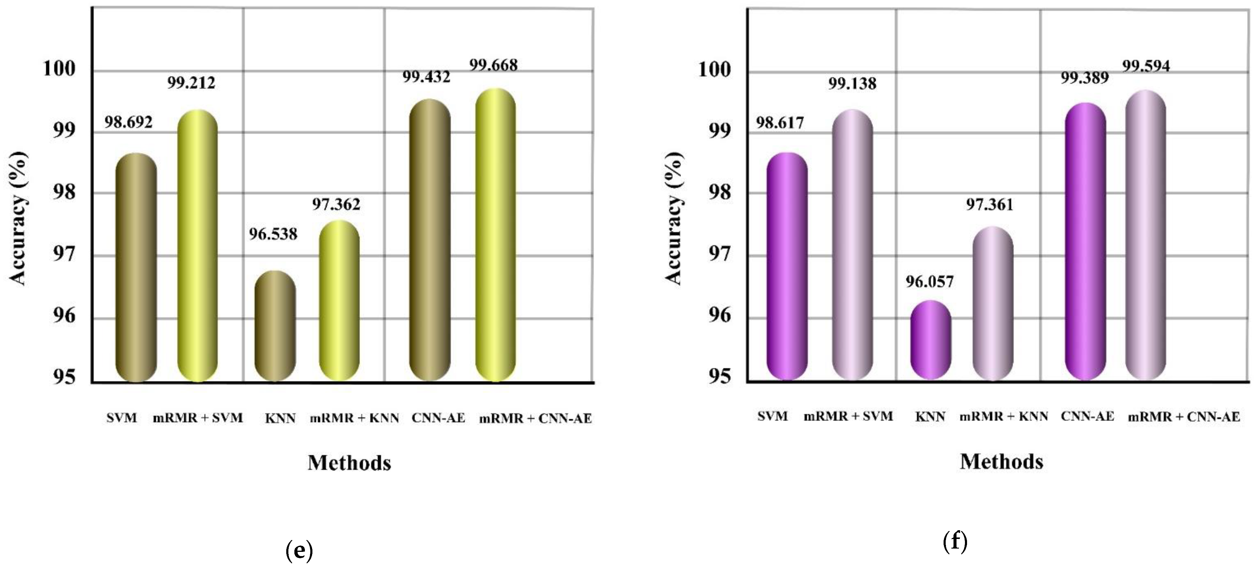
Figure 7 shows the results of the classifier algorithms with the mRMR feature selection method for the different problem classifications in the Bonn dataset. Figure 7 shows that using the mRMR method has increased the efficiency of classifier algorithms in epileptic seizure detection.
Table 9 shows the results of the proposed method for the Freiburg dataset. As shown in Table 9, the CNN-AE algorithm has been able to achieve the highest accuracy compared to other classifier algorithms when using mRMR.
Figure 8 shows the accuracy of various classifier algorithms with or without the mRMR method. As demonstrated in Table 7, Table 8 and Table 9, the proposed CNN-AE model has the highest detection accuracy for the Bonn and Freiburg datasets.

6. Discussion

This study provides a CADS for epileptic seizure detection via EEG signals using FD features and the proposed CNN-AE method. The proposed CADS include four sections: preprocessing, feature extraction, feature selection, and DL-based classification. First, the EEG signals of both datasets were decomposed into different time windows. Afterward, the DT-CWT technique was used for EEG signal decomposition into different sub-bands. In addition, the NS 13/19 and QS 14/14 filters were used for simulation of the DT-CWT.
Previous studies have indicated that EEG signals have a chaotic nature. Accordingly, using nonlinear feature extraction techniques, e.g., entropies [26], LLE [27], FDs [50,51,52,53,54,55,56,57,58,59,60,61,62,63,64,65,66,67,68,69], etc., leads to CADS performance enhancement in epileptic seizure detection [69]. Thereby, in the feature extraction step, different FD features are extracted from DT-CWT sub-bands. For the first time, different FD feature extraction methods are combined in this study, and this is considered to be the novelty of this paper.
In the following step, in order to reduce the size of the feature matrix, the mRMR method is used. In this step, the proposed feature selection method extracted 25 features.
In the final step, various machine learning (ML) and DL algorithms are used to classify the input data. The classifier methods consist of KNN, SVM, and CNN-AE methods. The CNN-AE method with proposed layers is another novelty of the paper. As previously mentioned, this architecture has two inputs, one of them is for applying raw EEG signals to the model, and the other input is for applying FD features. In the classification section, in order to calculate valid results, K-Fold with k = 10 is used. The CNN-AE architecture of this study is a feature fusion method since the FD-based handcrafted features and DL features are combined in this method to increase the accuracy of epileptic seizure detection. For the Bonn dataset, the proposed method achieved 99.736% accuracy for two-class classification problems and 99.594% accuracy for three-class classification problem. In addition, the proposed method on the Freiburg dataset achieved 99.176% accuracy. The experiment results show that the proposed method for both datasets achieved satisfactory results.

7. Conclusions and Future Works

Epilepsy is among a group of neural brain disorders taking place at different ages with various symptoms. If not diagnosed in the first stages, epileptic seizures will develop further [1,2,3,4,5]. Thereby, diagnosis of epileptic seizures in the first stages is of paramount importance for specialist physicians [6]. There have been various methods introduced to date for the early diagnosis of epileptic seizures. Among these methods, the recording of EEG signals is crucial for specialist physicians and neurologists. The EEG signals include important information regarding brain function at the time of epileptic seizures, which is significantly important for physicians. Recording EEG signals for epileptic seizure diagnosis is carried out in a long-term form, such that physicians cannot precisely examine all signals in detail. In addition, many factors, e.g., different artifacts in EEG signals, contribute to the fact that physicians encounter challenges in epileptic seizure detection.
In order to overcome the aforementioned obstacles, different AI methods are provided to help epileptic seizure diagnosis via EEG signals, and numerous investigations are being conducted. The AI techniques consist of various ML and DL methods. Each of these methods has some drawbacks and benefits.
This paper provides a novel CADS for epileptic seizure detection in EEG signals using FD features and a CNN-AE model with proposed layers. In this study, the steps of CADS for epileptic seizure detection from EEG signals include preprocessing, feature extraction, feature selection, and classification. Firstly, the Bonn and Freiburg datasets were used for experiments. During preprocessing, a band-pass filter (BPF) with 0.5–60 Hz cut-off frequency was employed for removal of artifacts in the EEG signals. In the next step, the EEG signals of the datasets were segmented into different time windows. For this, each EEG signal was segmented into time windows of 5 s and 4 s for the Bonn and Freiburg datasets, respectively. The DT-CWT with QS 14/14 and NS 13/19 filters was then used to decompose the EEG signals into different sub-bands. Feature extraction was performed employing various FD techniques. This step is the first innovation of the paper. Then, the mRMR technique was used for feature selection and the number of features was reduced to 25. The classification was eventually carried out using various ML models and a CNN-AE model, where the CNN-AE model with proposed layers is another novelty of the paper. The experiment results shows that the proposed CADS achieved the highest accuracy. Table 10 and Table 11 display the related works on epileptic seizure detection in EEG signals using the Bonn and Freiburg datasets, respectively.
As shown in Table 10 and Table 11, the proposed method has been able to achieve satisfactory results compared to previous work. The proposed method includes a combination of the most important preprocessing, feature extraction, feature selection, and classification methods for epileptic seizure detection. This has improved the efficiency of the proposed method compared to related work.
The proposed method has higher accuracy than other methods used in practical applications in epileptic seizure detection in EEG signals, such that it can be implemented on hardware platforms such as field programmable gate array (FPGA) [108,109,110] and employed in health centers as an auxiliary tool for quick epileptic seizure diagnosis [111].
In future works, we could use various CNN-AE models such as convolutional De-noising AE (CNN-DAE) [112,113] models for epileptic seizure detection. First, the EEG signals were converted to 2D images using the short-time Fourier transform (STFT) technique and then applied to one of the inputs of the CNN-AE model [114]. Then, various 2D features of STFT were extracted and applied to the other input of the CNN-AE model [115]. Another future study is using local binary pattern (LBP) feature extraction methods [116,117], such that the EEG signals of LBP features are extracted and applied to the CNN-AE input. For future works, we can use new deep feature fusion methods for epileptic seizure diagnosis using EEG signals [118,119]. Another future study is using advanced DL models for epileptic seizure detection in EEG signals [120,121,122,123,124,125,126].

Author Contributions

Conceptualization, A.M. and A.Z.; methodology, A.Z., A.M. and M.Y.; software, A.M.; validation, R.A. and M.Y.; formal analysis, A.M., R.A., A.Z. and M.Y.; resources, A.Z. and A.M.; writing—original draft preparation, A.M. and R.A.; writing—review and editing, A.M., A.Z., M.Y. and R.A.; visualization, A.Z., A.M. and R.A. All authors have read and agreed to the published version of the manuscript.

Funding

This research received no external funding.

Institutional Review Board Statement

Not applicable.

Informed Consent Statement

Not applicable.

Data Availability Statement

Not applicable.

Conflicts of Interest

The authors declare no conflict of interest.

References

  1. Litt, B.; Echauz, J. Prediction of epileptic seizures. Lancet Neurol. 2002, 1, 22–30. [Google Scholar] [CrossRef]
  2. Kumar, Y.; Dewal, M.L.; Anand, R.S. Epileptic seizures detection in EEG using DWT-based ApEn and artificial neural network. Signal Image Video Process. 2014, 8, 1323–1334. [Google Scholar] [CrossRef]
  3. Spagnoli, C.; Fusco, C.; Pisani, F. Rett Syndrome Spectrum in Monogenic Developmental-Epileptic Encephalopathies and Epilepsies: A Review. Genes 2021, 12, 1157. [Google Scholar] [CrossRef]
  4. Hatano, K.; Fujimoto, A.; Inenaga, C.; Otsuki, Y.; Enoki, H.; Okanishi, T. Non-Ruptured Temporal Lobe Dermoid Cyst Concomitant with Focal Cortical Dysplasia Causing Temporal Lobe Epilepsy—A Case Report and Literature Review. Brain Sci. 2021, 11, 1136. [Google Scholar] [CrossRef]
  5. Shoeibi, A.; Khodatars, M.; Ghassemi, N.; Jafari, M.; Moridian, P.; Alizadehsani, R.; Panahiazar, M.; Khozeimeh, F.; Zare, A.; Hosseini-Nejad, H.; et al. Epileptic Seizures Detection Using Deep Learning Techniques: A Review. Int. J. Environ. Res. Public Health 2021, 18, 5780. [Google Scholar] [CrossRef]
  6. Tsiouris, Κ.Μ.; Pezoulas, V.C.; Zervakis, M.; Konitsiotis, S.; Koutsouris, D.D.; Fotiadis, D.I. A long short-term memory deep learning network for the prediction of epileptic seizures using EEG signals. Comput. Biol. Med. 2018, 99, 24–37. [Google Scholar] [CrossRef]
  7. Shoeibi, A.; Ghassemi, N.; Khodatars, M.; Jafari, M.; Moridian, P.; Alizadehsani, R.; Khadem, A.; Kong, Y.; Zare, A.; Gorriz, J.M.; et al. Applications of Epileptic Seizures Detection in Neuroimaging Modalities Using Deep Learning Techniques: Methods, Challenges, and Future Works. arXiv 2021, arXiv:2105.14278. [Google Scholar]
  8. Pittau, F.; Grouiller, F.; Spinelli, L.; Seeck, M.; Michel, C.M.; Vulliemoz, S. The role of functional neuroimaging in pre-surgical epilepsy evaluation. Front. Neurol. 2014, 5, 31. [Google Scholar] [CrossRef] [Green Version]
  9. Cendes, F.; Theodore, W.H.; Brinkmann, B.H.; Sulc, V.; Cascino, G.D. Neuroimaging of epilepsy. Handb. Clin. Neurol. 2016, 136, 985–1014. [Google Scholar]
  10. Gross, D.W. Diffusion tensor imaging in temporal lobe epilepsy. Epilepsia 2011, 52, 32–34. [Google Scholar] [CrossRef] [PubMed]
  11. Jang, S.W.; Lee, S.H. Detection of epileptic seizures using wavelet transform, peak extraction and PSR from EEG signals. Symmetry 2020, 12, 1239. [Google Scholar] [CrossRef]
  12. Abiyev, R.; Arslan, M.; Bush Idoko, J.; Sekeroglu, B.; Ilhan, A. Identification of epileptic EEG signals using convolutional neural networks. Appl. Sci. 2020, 10, 4089. [Google Scholar] [CrossRef]
  13. San-Segundo, R.; Gil-Martín, M.; D’Haro-Enríquez, L.F.; Pardo, J.M. Classification of epileptic EEG recordings using signal transforms and convolutional neural networks. Comput. Biol. Med. 2019, 109, 148–158. [Google Scholar] [CrossRef]
  14. Gu, Y.; Cleeren, E.; Dan, J.; Claes, K.; Van Paesschen, W.; Van Huffel, S.; Hunyadi, B. Comparison between scalp EEG and behind-the-ear EEG for development of a wearable seizure detection system for patients with focal epilepsy. Sensors 2018, 18, 29. [Google Scholar] [CrossRef] [PubMed] [Green Version]
  15. Shoeibi, A.; Sadeghi, D.; Moridian, P.; Ghassemi, N.; Heras, J.; Alizadehsani, R.; Khadem, A.; Kong, Y.; Nahavandi, S.; Gorriz, J.M. Automatic Diagnosis of Schizophrenia using EEG Signals and CNN-LSTM Models. arXiv 2021, arXiv:2109.01120. [Google Scholar] [CrossRef]
  16. Alizadehsani, R.; Roshanzamir, M.; Hussain, S.; Khosravi, A.; Koohestani, A.; Zangooei, M.H.; Abdar, M.; Beykikhoshk, A.; Shoeibi, A.; Zare, A.; et al. Handling of uncertainty in medical data using machine learning and probability theory techniques: A review of 30 years (1991–2020). Ann. Oper. Res. 2021, 1–42. [Google Scholar] [CrossRef] [PubMed]
  17. Sadeghi, D.; Shoeibi, A.; Ghassemi, N.; Moridian, P.; Khadem, A.; Alizadehsani, R.; Teshnehlab, M.; Gorriz, J.M.; Nahavandi, S. An Overview on Artificial Intelligence Techniques for Diagnosis of Schizophrenia Based on Magnetic Resonance Imaging Modalities: Methods, Challenges, and Future Works. arXiv 2021, arXiv:2103.03081. [Google Scholar]
  18. Varone, G.; Gasparini, S.; Ferlazzo, E.; Ascoli, M.; Tripodi, G.G.; Zucco, C.; Calabrese, B.; Cannataro, M.; Aguglia, U. A Comprehensive Machine-Learning-Based Software Pipeline to Classify EEG Signals: A Case Study on PNES vs. Control Subjects. Sensors 2020, 20, 1235. [Google Scholar] [CrossRef] [Green Version]
  19. Tzallas, A.T.; Tsipouras, M.G.; Tsalikakis, D.G.; Karvounis, E.C.; Astrakas, L.; Konitsiotis, S.; Tzaphlidou, M. Automated Epileptic Seizure Detection Methods: A Review Study; Books on Demand: Norderstedt, Germany, 2012. [Google Scholar]
  20. Assi, E.B.; Nguyen, D.K.; Rihana, S.; Sawan, M. Towards accurate prediction of epileptic seizures: A review. Biomed. Signal Process. Control 2017, 34, 144–157. [Google Scholar] [CrossRef]
  21. Boonyakitanont, P.; Lek-Uthai, A.; Chomtho, K.; Songsiri, J. A review of feature extraction and performance evaluation in epileptic seizure detection using EEG. Biomed. Signal Process. Control 2020, 57, 101702. [Google Scholar] [CrossRef] [Green Version]
  22. Sriraam, N.; Raghu, S.; Tamanna, K.; Narayan, L.; Khanum, M.; Hegde, A.S.; Kumar, A.B. Automated epileptic seizures detection using multi-features and multilayer perceptron neural network. Brain Inform. 2018, 5, 1–10. [Google Scholar] [CrossRef]
  23. Al Ghayab, H.R.; Li, Y.; Siuly, S.; Abdulla, S. Epileptic seizures detection in EEGs blending frequency domain with information gain technique. Soft Comput. 2019, 23, 227–239. [Google Scholar] [CrossRef]
  24. Tzallas, A.T.; Tsipouras, M.G.; Fotiadis, D.I. Epileptic seizure detection in EEGs using time–frequency analysis. IEEE Trans. Inf. Technol. Biomed. 2009, 13, 703–710. [Google Scholar] [CrossRef] [PubMed]
  25. Wang, L.; Xue, W.; Li, Y.; Luo, M.; Huang, J.; Cui, W.; Huang, C. Automatic epileptic seizure detection in EEG signals using multi-domain feature extraction and nonlinear analysis. Entropy 2017, 19, 222. [Google Scholar] [CrossRef] [Green Version]
  26. Raghu, S.; Sriraam, N.; Kumar, G.P.; Hegde, A.S. A novel approach for real-time recognition of epileptic seizures using minimum variance modified fuzzy entropy. IEEE Trans. Biomed. Eng. 2018, 65, 2612–2621. [Google Scholar] [CrossRef]
  27. Korda, A.I.; Asvestas, P.A.; Matsopoulos, G.K.; Ventouras, E.M.; Smyrnis, N. Automatic identification of eye movements using the largest lyapunov exponent. Biomed. Signal Process. Control 2018, 41, 10–20. [Google Scholar] [CrossRef]
  28. Li, Q.; Gao, J.; Huang, Q.; Wu, Y.; Xu, B. Distinguishing Epileptiform Discharges from Normal Electroencephalograms Using Scale-Dependent Lyapunov Exponent. Front. Bioeng. Biotechnol. 2020, 8, 1006. [Google Scholar] [CrossRef] [PubMed]
  29. EEG Time Series Data (Department of Epileptology University of Bonn, Germany). Available online: http://epileptologie-bonn.de/cms/front_content.php?idcat=193&lang=3&changelang=3 (accessed on 25 September 2021).
  30. EEG Database. Available online: https://epilepsy.uni-freiburg.de/freiburg-seizure-prediction-project/eeg-database/ (accessed on 10 December 2021).
  31. Slimen, I.B.; Boubchir, L.; Mbarki, Z.; Seddik, H. EEG epileptic seizure detection and classification based on dual-tree complex wavelet transform and machine learning algorithms. J. Biomed. Res. 2020, 34, 151. [Google Scholar] [CrossRef]
  32. Khan, A.T.; Khan, Y.U. Dual tree complex wavelet transform based analysis of epileptiform discharges. Int. J. Inf. Technol. 2018, 10, 543–550. [Google Scholar] [CrossRef]
  33. Kingsbury, N.G. The dual-tree complex wavelet transform: A new technique for shift invariance and directional filters. IEEE Digit. Signal Process. Workshop 1998, 86, 120–131. [Google Scholar]
  34. Das, A.B.; Bhuiyan, M.I.H.; Alam, S.S. A statistical method for automatic detection of seizure and epilepsy in the dual tree complex wavelet transform domain. In Proceedings of the 2014 International Conference on Informatics, Electronics & Vision (ICIEV), Dhaka, Bangladesh, 23–24 May 2014; pp. 1–6. [Google Scholar]
  35. Hassan, A.R.; Bhuiyan, M.I.H. Dual tree complex wavelet transform for sleep state identification from single channel electroencephalogram. In Proceedings of the 2015 IEEE International Conference on Telecommunications and Photonics (ICTP), Dhaka, Bangladesh, 26–28 December 2015; pp. 1–5. [Google Scholar]
  36. Bhuiyan, M.I.H.; Das, A.B. A subband correlation-based method for the automatic detection of epilepsy and seizure in the dual tree complex wavelet transform domain. In Proceedings of the 2014 IEEE Conference on Biomedical Engineering and Sciences (IECBES), Kuala Lumpur, Malaysia, 8–10 December 2014; pp. 811–816. [Google Scholar]
  37. Madan, S.; Srivastava, K.; Sharmila, A.; Mahalakshmi, P. A case study on Discrete Wavelet Transform based Hurst exponent for epilepsy detection. J. Med. Eng. Technol. 2018, 42, 9–17. [Google Scholar] [CrossRef]
  38. Esteller, R.; Vachtsevanos, G.; Echauz, J.; Litt, B. A comparison of waveform fractal dimension algorithms. IEEE Trans. Circuits Syst. I Fundam. Theory Appl. 2001, 48, 177–183. [Google Scholar] [CrossRef] [Green Version]
  39. Raghavendra, B.S.; Dutt, N.D. Computing fractal dimension of signals using multiresolution box-counting method. Int. J. Inf. Math. Sci. 2010, 6, 50–65. [Google Scholar]
  40. Majkowski, A.; Kołodziej, M.; Rak, R.J.; Rysz, A. Implementation of ECoG Signal Energy, Entropy and Fractal Dimension for Spike Detection. In Proceedings of the 2018 IEEE International Symposium on Medical Measurements and Applications (MeMeA), Rome, Italy, 11–13 June 2018; pp. 1–6. [Google Scholar]
  41. Croce, P.; Quercia, A.; Costa, S.; Zappasodi, F. Circadian rhythms in fractal features of EEG signals. Front. Physiol. 2018, 9, 1567. [Google Scholar] [CrossRef] [Green Version]
  42. Gruszczyńska, I.; Mosdorf, R.; Sobaniec, P.; Żochowska-Sobaniec, M.; Borowska, M. Epilepsy identification based on EEG signal using RQA method. Adv. Med. Sci. 2019, 64, 58–64. [Google Scholar] [CrossRef]
  43. Maragos, P.; Sun, F.K. Measuring the fractal dimension of signals: Morphological covers and iterative optimization. IEEE Trans. Signal Process. 1993, 41, 108. [Google Scholar] [CrossRef]
  44. Zhang, Z.; Wen, T.; Huang, W.; Wang, M.; Li, C. Automatic epileptic seizure detection in EEGs using MF-DFA, SVM based on cloud computing. J. X-ray Sci. Technol. 2017, 25, 261–272. [Google Scholar] [CrossRef]
  45. Theiler, J. Estimating fractal dimension. JOSA A 1990, 7, 1055–1073. [Google Scholar] [CrossRef] [Green Version]
  46. Cai, Y.; Huang, T.; Hu, L.; Shi, X.; Xie, L.; Li, Y. Prediction of lysine ubiquitination with mRMR feature selection and analysis. Amino Acids 2012, 42, 1387–1395. [Google Scholar] [CrossRef] [PubMed]
  47. Liao, Y.; Vemuri, V.R. Use of k-nearest neighbor classifier for intrusion detection. Comput. Secur. 2002, 21, 439–448. [Google Scholar] [CrossRef]
  48. Noble, W.S. What is a support vector machine? Nat. Biotechnol. 2006, 24, 1565–1567. [Google Scholar] [CrossRef] [PubMed]
  49. Meyer, D.; Leisch, F.; Hornik, K. The support vector machine under test. Neurocomputing 2003, 55, 169–186. [Google Scholar] [CrossRef]
  50. Wijayanto, I.; Rizal, A.; Humairani, A. Seizure detection based on EEG signals using katz fractal and SVM classifiers. In Proceedings of the 2019 5th International Conference on Science in Information Technology (ICSITech), Yogyakarta, Indonesia, 23–24 October 2019; pp. 78–82. [Google Scholar]
  51. Yuan, Q.; Zhou, W.; Liu, Y.; Wang, J. Epileptic seizure detection with linear and nonlinear features. Epilepsy Behav. 2012, 24, 415–421. [Google Scholar] [CrossRef] [PubMed]
  52. Zhang, Y.; Zhou, W.; Yuan, S.; Yuan, Q. Seizure detection method based on fractal dimension and gradient boosting. Epilepsy Behav. 2015, 43, 30–38. [Google Scholar] [CrossRef]
  53. Yang, S.; Li, G.; Lu, J.; Sun, Y.; Huang, Z. EEG-Based Seizure Diagnosis Using Discriminative Fractal Features from Feature Selection. In Proceedings of the International Conference on Intelligent Computing, Nanchang, China, 3–6 August 2019; pp. 436–447. [Google Scholar]
  54. Moctezuma, L.A.; Molinas, M. Classification of low-density EEG for epileptic seizures by energy and fractal features based on EMD. J. Biomed. Res. 2020, 34, 180. [Google Scholar] [CrossRef]
  55. Uthayakumar, R.; Easwaramoorthy, D. Epileptic seizure detection in EEG signals using multifractal analysis and wavelet transform. Fractals 2013, 21, 1350011. [Google Scholar] [CrossRef]
  56. Humairani, A.; Atmojo, B.S.; Wijayanto, I.; Hadiyoso, S. Fractal Based Feature Extraction Method for Epileptic Seizure Detection in Long-Term EEG Recording. In Journal of Physics: Conference Series; IOP Publishing: Bristol, UK, 2021; Volume 1844, p. 012019. [Google Scholar]
  57. Sikdar, D.; Roy, R.; Mahadevappa, M. Epilepsy and seizure characterisation by multifractal analysis of EEG subbands. Biomed. Signal Process. Control 2018, 41, 264–270. [Google Scholar] [CrossRef]
  58. Dalal, M.; Tanveer, M.; Pachori, R.B. Automated identification system for focal EEG signals using fractal dimension of FAWT-based sub-bands signals. In Machine Intelligence and Signal Analysis; Springer: Singapore, 2019; pp. 583–596. [Google Scholar]
  59. El-Kishky, A. Assessing entropy and fractal dimensions as discriminants of seizures in EEG time series. In Proceedings of the 2012 11th International Conference on Information Science, Signal Processing and their Applications (ISSPA), Montreal, QC, Canada, 2–5 July 2012; pp. 92–96. [Google Scholar]
  60. Jacob, J.E.; Gopakumar, K. Automated diagnosis of encephalopathy using fractal dimensions of EEG sub-bands. In Proceedings of the 2018 IEEE Recent Advances in Intelligent Computational Systems (RAICS), Thiruvananthapuram, India, 6–8 December 2018; pp. 94–97. [Google Scholar]
  61. Dash, D.P.; Kolekar, M.H. Epileptic seizure detection based on EEG signal analysis using hierarchy based Hidden Markov Model. In Proceedings of the 2017 International Conference on Advances in Computing, Communications and Informatics (ICACCI), Udupi, India, 13–16 September 2017; pp. 1114–1120. [Google Scholar]
  62. Easwaramoorthy, D.; Uthayakumar, R. Improved generalized fractal dimensions in the discrimination between healthy and epileptic EEG signals. J. Comput. Sci. 2011, 2, 31–38. [Google Scholar] [CrossRef]
  63. Sharma, M.; Pachori, R.B.; Acharya, U.R. A new approach to characterize epileptic seizures using analytic time-frequency flexible wavelet transform and fractal dimension. Pattern Recognit. Lett. 2017, 94, 172–179. [Google Scholar] [CrossRef]
  64. Sharma, M.; Pachori, R.B. A novel approach to detect epileptic seizures using a combination of tunable-Q wavelet transform and fractal dimension. J. Mech. Med. Biol. 2017, 17, 1740003. [Google Scholar] [CrossRef]
  65. Jirka, J.; Prauzek, M.; Krejcar, O.; Kuca, K. Automatic epilepsy detection using fractal dimensions segmentation and GP–SVM classification. Neuropsychiatr. Dis. Treat. 2018, 14, 2439. [Google Scholar] [CrossRef] [Green Version]
  66. Wijayanto, I.; Hadiyoso, S.; Aulia, S.; Atmojo, B.S. Detecting Ictal and Interictal Condition of EEG Signal using Higuchi Fractal Dimension and Support Vector Machine. In Journal of Physics: Conference Series; IOP Publishing: Bristol, UK, 2020; Volume 1577, p. 012016. [Google Scholar]
  67. Dautov, Ç.P.; Özerdem, M.S. Epilepsy detection using a naive signal decomposition method combined with fractal dimension. In Proceedings of the 2018 26th Signal Processing and Communications Applications Conference (SIU), Izmir, Turkey, 2–5 May 2018; pp. 1–4. [Google Scholar]
  68. Diykh, M.; Abdulla, S.; Saleh, K.; Deo, R.C. Fractal dimension undirected correlation graph-based support vector machine model for identification of focal and non-focal electroencephalography signals. Biomed. Signal Process. Control 2019, 54, 101611. [Google Scholar] [CrossRef]
  69. Wijayanto, I.; Hartanto, R.; Nugroho, H.A. Higuchi and Katz Fractal Dimension for Detecting Interictal and Ictal State in Electroencephalogram Signal. In Proceedings of the 2019 11th International Conference on Information Technology and Electrical Engineering (ICITEE), Pattaya, Thailand, 10–11 October 2019; pp. 1–6. [Google Scholar]
  70. Li, M.; Chen, W.; Zhang, T. Automatic epileptic EEG detection using DT-CWT-based non-linear features. Biomed. Signal Process. Control 2017, 34, 114–125. [Google Scholar] [CrossRef]
  71. Ghassemi, N.; Shoeibi, A.; Rouhani, M.; Hosseini-Nejad, H. Epileptic seizures detection in EEG signals using TQWT and ensemble learning. In Proceedings of the 2019 9th International Conference on Computer and Knowledge Engineering (ICCKE), Mashhad, Iran, 24–25 October 2019; pp. 403–408. [Google Scholar]
  72. Shoeibi, A.; Khodatars, M.; Alizadehsani, R.; Ghassemi, N.; Jafari, M.; Moridian, P.; Khadem, A.; Sadeghi, D.; Hussain, S.; Zare, A.; et al. Automated detection and forecasting of covid-19 using deep learning techniques: A review. arXiv 2020, arXiv:2007.10785. [Google Scholar]
  73. Khodatars, M.; Shoeibi, A.; Sadeghi, D.; Ghaasemi, N.; Jafari, M.; Moridian, P.; Khadem, A.; Alizadehsani, R.; Zare, A.; Kong, Y.; et al. Deep learning for neuroimaging-based diagnosis and rehabilitation of autism spectrum disorder: A review. arXiv 2020, arXiv:2007.01285. [Google Scholar] [CrossRef]
  74. Ayoobi, N.; Sharifrazi, D.; Alizadehsani, R.; Shoeibi, A.; Gorriz, J.M.; Moosaei, H.; Khosravi, A.; Nahavandi, S.; Chofreh, A.G.; Goni, F.A.; et al. Time Series Forecasting of New Cases and New Deaths Rate for COVID-19 using Deep Learning Methods. arXiv 2021, arXiv:2104.15007. [Google Scholar] [CrossRef] [PubMed]
  75. Mohammadpoor, M.; Shoeibi, A.; Shojaee, H. A hierarchical classification method for breast tumor detection. Iran. J. Med. Phys. 2016, 13, 261–268. [Google Scholar]
  76. Yildirim, O.; San Tan, R.; Acharya, U.R. An efficient compression of ECG signals using deep convolutional autoencoders. Cogn. Syst. Res. 2018, 52, 198–211. [Google Scholar] [CrossRef]
  77. Chen, M.; Shi, X.; Zhang, Y.; Wu, D.; Guizani, M. Deep features learning for medical image analysis with convolutional autoencoder neural network. IEEE Trans. Big Data 2017, 7, 750–758. [Google Scholar] [CrossRef]
  78. Pedregosa, F.; Varoquaux, G.; Gramfort, A.; Michel, V.; Thirion, B.; Grisel, O.; Blondel, M.; Prettenhofer, P.; Weiss, R.; Dubourg, V.; et al. Scikit-learn: Machine learning in Python. J. Mach. Learn. Res. 2011, 12, 2825–2830. [Google Scholar]
  79. Gulli, A.; Pal, S. Deep Learning with Keras; Packt Publishing Ltd.: Birmingham, UK, 2017. [Google Scholar]
  80. Zhang, T.; Han, Z.; Chen, X.; Chen, W. Subbands and cumulative sum of subbands based nonlinear features enhance the performance of epileptic seizure detection. Biomed. Signal Process. Control 2021, 69, 102827. [Google Scholar] [CrossRef]
  81. Jindal, K.; Upadhyay, R.; Singh, H.S. Application of tunable-Q wavelet transform based nonlinear features in epileptic seizure detection. Analog Integr. Circuits Signal Process. 2019, 100, 437–452. [Google Scholar] [CrossRef]
  82. Thara, D.K.; PremaSudha, B.G.; Xiong, F. Auto-detection of epileptic seizure events using deep neural network with different feature scaling techniques. Pattern Recognit. Lett. 2019, 128, 544–550. [Google Scholar]
  83. David, S.A.; Machado, J.A.T.; Inácio, C.M.; Valentim, C.A. A combined measure to differentiate EEG signals using fractal dimension and MFDFA-Hurst. Commun. Nonlinear Sci. Numer. Simul. 2020, 84, 105170. [Google Scholar] [CrossRef]
  84. Ballester, P.; Araujo, R.M. On the performance of GoogLeNet and AlexNet applied to sketches. In Proceedings of the Thirtieth AAAI Conference on Artificial Intelligence, Phoenix, AZ, USA, 12–17 February 2016. [Google Scholar]
  85. Tzimourta, K.D.; Tzallas, A.T.; Giannakeas, N.; Astrakas, L.G.; Tsalikakis, D.G.; Angelidis, P.; Tsipouras, M.G. A robust methodology for classification of epileptic seizures in EEG signals. Health Technol. 2019, 9, 135–142. [Google Scholar] [CrossRef]
  86. Singh, G.; Kaur, M.; Singh, B. Detection of epileptic seizure EEG signal using multiscale entropies and complete ensemble empirical mode decomposition. Wirel. Pers. Commun. 2021, 116, 845–864. [Google Scholar] [CrossRef]
  87. Atal, D.K.; Singh, M. A hybrid feature extraction and machine learning approaches for epileptic seizure detection. Multidimens. Syst. Signal Process. 2020, 31, 503–525. [Google Scholar] [CrossRef]
  88. Deriche, M.; Arafat, S.; Al-Insaif, S.; Siddiqui, M. Eigenspace time frequency based features for accurate seizure detection from EEG data. IRBM 2019, 40, 122–132. [Google Scholar] [CrossRef]
  89. Aliyu, I.; Lim, C.G. Selection of optimal wavelet features for epileptic EEG signal classification with LSTM. Neural Comput. Appl. 2021, 1–21. [Google Scholar] [CrossRef]
  90. Liu, J.; Woodson, B. Deep learning classification for epilepsy detection using a single channel electroencephalography (EEG). In Proceedings of the 2019 3rd International Conference on Deep Learning Technologies, Xiamen, China, 5–7 July 2019; pp. 23–26. [Google Scholar]
  91. Daoud, H.G.; Abdelhameed, A.M.; Bayoumi, M. Automatic epileptic seizure detection based on empirical mode decomposition and deep neural network. In Proceedings of the 2018 IEEE 14th International Colloquium on Signal Processing & Its Applications (CSPA), Penang, Malaysia, 9–10 March 2018; pp. 182–186. [Google Scholar]
  92. Abdel-Ghaffar, E.A. Effect of tuning TQWT parameters on epileptic seizure detection from EEG signals. In Proceedings of the 2017 12th International Conference on Computer Engineering and Systems (ICCES), Cairo, Egypt, 19–20 December 2017; pp. 47–51. [Google Scholar]
  93. Gupta, V.; Bhattacharyya, A.; Pachori, R.B. Classification of seizure and non-seizure EEG signals based on EMD-TQWT method. In Proceedings of the 2017 22nd International Conference on Digital Signal Processing (DSP), London, UK, 23–25 August 2017; pp. 1–5. [Google Scholar]
  94. Zhang, T.; Chen, W.; Li, M. Generalized Stockwell transform and SVD-based epileptic seizure detection in EEG using random forest. Biocybern. Biomed. Eng. 2018, 38, 519–534. [Google Scholar] [CrossRef]
  95. Waqar, H.; Xiang, J.; Zhou, M.; Hu, T.; Ahmed, B.; Shapor, S.H.; Iqbal, M.S.; Raheel, M. Towards classifying epileptic seizures using entropy variants. In Proceedings of the 2019 IEEE Fifth International Conference on Big Data Computing Service and Applications (BigDataService), Newark, CA, USA, 4–9 April 2019; pp. 296–300. [Google Scholar]
  96. Truong, N.D.; Kavehei, O. Low precision electroencephalogram for seizure detection with convolutional neural network. In Proceedings of the 2019 IEEE International Conference on Artificial Intelligence Circuits and Systems (AICAS), Hsinchu, Taiwan, 18–20 March 2019; pp. 299–301. [Google Scholar]
  97. Nassralla, M.; Haidar, M.; Alawieh, H.; El Hajj, A.; Dawy, Z. Patient-aware EEG-based feature and classifier selection for e-health epileptic seizure prediction. In Proceedings of the 2018 IEEE Global Communications Conference (GLOBECOM), Abu Dhabi, United Arab Emirates, 9–13 December 2018; pp. 1–6. [Google Scholar]
  98. Yuan, Q.; Zhou, W.; Zhang, L.; Zhang, F.; Xu, F.; Leng, Y.; Wei, D.; Chen, M. Epileptic seizure detection based on imbalanced classification and wavelet packet transform. Seizure 2017, 50, 99–108. [Google Scholar] [CrossRef] [PubMed]
  99. Zhou, M.; Tian, C.; Cao, R.; Wang, B.; Niu, Y.; Hu, T.; Guo, H.; Xiang, J. Epileptic seizure detection based on EEG signals and CNN. Front. Neuroinform. 2018, 12, 95. [Google Scholar] [CrossRef] [Green Version]
  100. Mahmoodian, N.; Boese, A.; Friebe, M.; Haddadnia, J. Epileptic seizure detection using cross-bispectrum of electroencephalogram signal. Seizure 2019, 66, 4–11. [Google Scholar] [CrossRef] [Green Version]
  101. Martinez-del-Rincon, J.; Santofimia, M.J.; del Toro, X.; Barba, J.; Romero, F.; Navas, P.; Lopez, J.C. Non-linear classifiers applied to EEG analysis for epilepsy seizure detection. Expert Syst. Appl. 2017, 86, 99–112. [Google Scholar] [CrossRef] [Green Version]
  102. Jaafar, S.T.; Mohammadi, M. Epileptic Seizure Detection using Deep Learning Approach. UHD J. Sci. Technol. 2019, 3, 41–50. [Google Scholar] [CrossRef] [Green Version]
  103. Truong, N.D.; Nguyen, A.D.; Kuhlmann, L.; Bonyadi, M.R.; Yang, J.; Ippolito, S.; Kavehei, O. Integer convolutional neural network for seizure detection. IEEE J. Emerg. Sel. Top. Circuits Syst. 2018, 8, 849–857. [Google Scholar] [CrossRef]
  104. Abbaszadeh, B.; Yagoub, M.C. Optimum Window Size and Overlap for Robust Probabilistic Prediction of Seizures with iEEG. In Proceedings of the 2019 IEEE Conference on Computational Intelligence in Bioinformatics and Computational Biology (CIBCB), Siena, Italy, 9–11 July 2019; pp. 1–5. [Google Scholar]
  105. Mohammadi, M.; Khan, N.A.; Pouyan, A.A. Automatic seizure detection using a highly adaptive directional time–frequency distribution. Multidimens. Syst. Signal Process. 2018, 29, 1661–1678. [Google Scholar] [CrossRef]
  106. Sun, C.; Cui, H.; Zhou, W.; Nie, W.; Wang, X.; Yuan, Q. Epileptic seizure detection with EEG textural features and imbalanced classification based on EasyEnsemble learning. Int. J. Neural Syst. 2019, 29, 1950021. [Google Scholar] [CrossRef] [PubMed]
  107. Abugabah, A.; AlZubi, A.A.; Al-Maitah, M.; Alarifi, A. Brain epilepsy seizure detection using bio-inspired krill herd and artificial alga optimized neural network approaches. J. Ambient. Intell. Humaniz. Comput. 2020, 12, 3317–3328. [Google Scholar] [CrossRef]
  108. Ahmadi-Dastgerdi, N.; Hosseini-Nejad, H.; Amiri, H.; Shoeibi, A.; Gorriz, J.M. A Vector Quantization-Based Spike Compression Approach Dedicated to Multichannel Neural Recording Microsystems. Int. J. Neural Syst. 2021. [Google Scholar] [CrossRef]
  109. Sahani, M.; Rout, S.K.; Dash, P.K. FPGA implementation of epileptic seizure detection using semisupervised reduced deep convolutional neural network. Appl. Soft Comput. 2021, 110, 107639. [Google Scholar] [CrossRef]
  110. Saidi, A.; Othman, S.B.; Kacem, W.; Saoud, S.B. FPGA Implementation of EEG Signal Analysis System for the Detection of epileptic seizure. In Proceedings of the 2018 International Conference on Advanced Systems and Electric Technologies (IC_ASET), Hammamet, Tunisia, 22–25 March 2018; pp. 415–420. [Google Scholar]
  111. Verma, N.; Shoeb, A.; Bohorquez, J.; Dawson, J.; Guttag, J.; Chandrakasan, A.P. A micro-power EEG acquisition SoC with integrated feature extraction processor for a chronic seizure detection system. IEEE J. Solid-State Circuits 2010, 45, 804–816. [Google Scholar] [CrossRef]
  112. Gondara, L. Medical image denoising using convolutional denoising autoencoders. In Proceedings of the 2016 IEEE 16th International Conference on Data Mining Workshops (ICDMW), Barcelona, Spain, 12–15 December 2016; pp. 241–246. [Google Scholar]
  113. Du, B.; Xiong, W.; Wu, J.; Zhang, L.; Zhang, L.; Tao, D. Stacked convolutional denoising auto-encoders for feature representation. IEEE Trans. Cybern. 2016, 47, 1017–1027. [Google Scholar] [CrossRef] [PubMed]
  114. Yuan, Y.; Xun, G.; Jia, K.; Zhang, A. A multi-view deep learning method for epileptic seizure detection using short-time fourier transform. In Proceedings of the 8th ACM International Conference on Bioinformatics, Computational Biology, and Health Informatics, Boston, MA, USA, 20–23 August 2017; pp. 213–222. [Google Scholar]
  115. Beeraka, S.M.; Kumar, A.; Sameer, M.; Ghosh, S.; Gupta, B. Accuracy Enhancement of Epileptic Seizure Detection: A Deep Learning Approach with Hardware Realization of STFT. Circuits Syst. Signal Process. 2021, 1–24. [Google Scholar] [CrossRef]
  116. Burrello, A.; Schindler, K.; Benini, L.; Rahimi, A. Hyperdimensional computing with local binary patterns: One-shot learning of seizure onset and identification of ictogenic brain regions using short-time ieeg recordings. IEEE Trans. Biomed. Eng. 2019, 67, 601–613. [Google Scholar] [CrossRef]
  117. Kumar, T.S.; Kanhangad, V.; Pachori, R.B. Classification of seizure and seizure-free EEG signals using local binary patterns. Biomed. Signal Process. Control 2015, 15, 33–40. [Google Scholar] [CrossRef]
  118. Huang, C.; Chen, W.; Chen, M.; Yuan, B. A Feature Fusion Framework and Its Application to Automatic Seizure Detection. IEEE Signal Process. Lett. 2021, 28, 753–757. [Google Scholar] [CrossRef]
  119. Hu, D.; Cao, J.; Lai, X.; Wang, Y.; Wang, S.; Ding, Y. Epileptic state classification by fusing hand-crafted and deep learning EEG features. IEEE Trans. Circuits Syst. II Express Briefs 2020, 68, 1542–1546. [Google Scholar] [CrossRef]
  120. Sharifrazi, D.; Alizadehsani, R.; Roshanzamir, M.; Joloudari, J.H.; Shoeibi, A.; Jafari, M.; Hussain, S.; Sani, Z.A.; Hasanzadeh, F.; Khozeimeh, F.; et al. Fusion of convolution neural network, support vector machine and Sobel filter for accurate detection of COVID-19 patients using X-ray images. Biomed. Signal Process. Control 2021, 68, 102622. [Google Scholar] [CrossRef]
  121. Baydokhty, M.E.; Zare, A.; Balochian, S. Performance of optimal hierarchical type 2 fuzzy controller for load–frequency system with production rate limitation and governor dead band. Alex. Eng. J. 2016, 55, 379–397. [Google Scholar] [CrossRef] [Green Version]
  122. Alizadehsani, R.; Sharifrazi, D.; Izadi, N.H.; Joloudari, J.H.; Shoeibi, A.; Gorriz, J.M.; Hussain, S.; Arco, J.E.; Sani, Z.A.; Khozeimeh, F.; et al. Uncertainty-aware semi-supervised method using large unlabelled and limited labeled COVID-19 data. arXiv 2021, arXiv:2102.06388. [Google Scholar]
  123. Shoeibi, A.; Khodatars, M.; Jafari, M.; Moridian, P.; Rezaei, M.; Alizadehsani, R.; Khozeimeh, F.; Gorriz, J.M.; Heras, J.; Panahiazar, M.; et al. Applications of Deep Learning Techniques for Automated Multiple Sclerosis Detection Using Magnetic Resonance Imaging: A Review. arXiv 2021, arXiv:2105.04881. [Google Scholar] [CrossRef] [PubMed]
  124. Khozeimeh, F.; Sharifrazi, D.; Izadi, N.H.; Joloudari, J.H.; Shoeibi, A.; Alizadehsani, R.; Gorriz, J.M.; Hussain, S.; Sani, Z.A.; Moosaei, H.; et al. Combining a convolutional neural network with autoencoders to predict the survival chance of COVID-19 patients. Sci. Rep. 2021, 11, 1–18. [Google Scholar] [CrossRef]
  125. Sharifrazi, D.; Alizadehsani, R.; Joloudari, J.H.; Shamshirband, S.; Hussain, S.; Sani, Z.A.; Hasanzadeh, F.; Shoaibi, A.; Dehzangi, A.; Alinejad-Rokny, H. CNN-KCL: Automatic Myocarditis Diagnosis using Convolutional Neural Network Combined with K-means Clustering. Preprints 2020. [Google Scholar] [CrossRef]
  126. Shoeibi, A.; Ghassemi, N.; Khodatars, M.; Moridian, P.; Alizadehsani, R.; Zare, A.; Khosravi, A.; Subasi, A.; Acharya, U.R.; Gorriz, J.M. Detection of Epileptic Seizures on EEG Signals Using ANFIS Classifier, Autoencoders and Fuzzy Entropies. arXiv 2021, arXiv:2109.04364. [Google Scholar] [CrossRef]
Figure 1. The block diagram of proposed method for epileptic seizure detection.
Bdcc 05 00078 g001
Figure 2. Exemplary EEGs from five samples of the Bonn dataset.
Bdcc 05 00078 g002
Figure 3. Exemplary EEGs from five samples of the Freiburg dataset.
Bdcc 05 00078 g003
Figure 4. DT-CWT wavelet conversion scheme with four decomposition steps.
Bdcc 05 00078 g004
Figure 5. Five frequency sub-bands of an EEG signal using DT-CWT.
Bdcc 05 00078 g005aBdcc 05 00078 g005b
Figure 6. Proposed CNN-AE model for epileptic seizure detection.
Bdcc 05 00078 g006
Figure 7. Results for the Bonn Dataset. (a): set A-E, (b): Set B-E, (c): set C-E, (d): set D-E, (e): set ABCD-E, (f): set AB-CD-E.
Bdcc 05 00078 g007aBdcc 05 00078 g007b
Figure 8. Results for the Freiburg dataset.
Bdcc 05 00078 g008
Table 1. Related works on diagnosis of epileptic seizures using FD features.
WorksDatasetPreprocessingFeature ExtractionFeature SelectionClassifier
[50]BonnDecomposing into 5 Sub-bandsKFDNASVM
[51]FreiburgSliding window, FilteringDBCNASLFN
[52]FreiburgFiltering, SegmentationFDNAGradient Boosting
[53]ClinicalFilteringGFDRun CoveringSVM
[54]CHB-MITSegmentation, EMDEnergy Distribution Features, FDsK MeansSVM
[55]BonnFiltering, DWTGFD, Rayni EntropyANOVANA
[56]CHB-MITFiltering, Windowing, EMDHFD, KFD, Sevcik--SVM
[57]BonnFiltering, DWTMF-DFAStatistical AnalysisSVM
[58]Bern-BarcelonaFAWTHFDKruskal–Wallis Statistical TestRELS-TSVM
[59]BonnFiltering, Segmentation, NormalizationShannon entropy, HFD, HETwo-sample t-testNA
[60]ClinicalFiltering, DWTHFD, KFDNASVM
[61]ClinicalFilteringAverage Entropy Feature and
Hjorth Parameters
ANOVAK Means
[62]ClinicalSegmentationGFD, Rényi EntropyANOVA--
[63]BonnFiltering, ATFFWTShift-invariance Property, Tunable Oscillatory Attribute, FDStudent’s t-testLS-SVM
[64]BonnFiltering, TQWTFDsStudent T-Test, SFSLS-SVM
[65]ClinicalFiltering, DWTFDsGASVM
[66]BonnDecompositionHFD--SVM
[67]BonnFiltering, Signal Decomposition Through Naive MethodHFD----
[68]BernSliding Window Technique, ClusteringUndirected Graph Construction- Fractal Dimension (FD-NG)--SCA-SVM
[69]Bonn--HFD, KFD--SVM
Table 2. Thorough explanation of five subsets of dataset.
SetsSubjects
Patient StageNum. of CasesNum. of DataLength of Segments
Set AEye Open51004097
Set BEye Closed51004097
Set CSeizure Free51004097
Set DSeizure Free51004097
Set ESeizure Activity51004097
Table 3. Further details about six problem classification.
RowClassificationsDescription
1A-EHealthy Control—Ictal
2B-EHealthy Control—Ictal
3C-EInterictal—Ictal
4D-EInterictal—Ictal
5ABCD-ENormal—Seizure
6AB-CD-EHealthy Control—Interictal—Seizure
Table 4. Further details about the Freiburg dataset.
PatientAgeGenderSeizure OriginSeizure TypeNumber of Seizures
115FemaleTemporalSP, CP4
238MaleFrontalSP, CP, GTC3
314MaleTemporalSP, CP5
426FemaleTemporalSP, CP, GTC5
516FemaleFrontalSP, CP, GTC5
631FemaleTemporalCP, GTC3
742FemaleTemporalSP, CP, GTC3
832FemaleTemporalSP, CP2
944MaleFrontalCP, GTC5
1047MaleFrontalSP, CP, GTC5
1110FemaleFrontalSP, CP, GTC4
1242FemaleFrontalSP, CP, GTC4
1322FemaleTemporalSP, CP, GTC2
1441FemaleTemporalCP, GTC4
1531MaleFrontalSP, CP, GTC4
1650FemaleTemporalSP, CP, GTC5
1728MaleTemporalSP, CP, GTC5
1825FemaleTemporalSP, CP5
1928FemaleFrontalSP, CP, GTC4
2033MaleTemporalSP, CP, GTC5
2113MaleTemporalSP, CP5
Table 5. Details of proposed CNN-AE method.
ArchitectureLayersFiltersKernel SizeStrideActivationNumber of Features
(Bonn Dataset)
Number of Features
(Freiburg Dataset)
EncoderInput Data--------8681024
Conv1D3271ReLU8681024
Max Pooling--41--217256
Dropout----Rate = 0.25--217256
Conv1D3271ReLU217256
Max Pooling--41--5464
DecoderConv1D3271ReLU5464
Up Sampling--41--216256
Conv1D3271ReLU216256
Up Sampling--41--8641024
Zero Pad--------8681024
Conv1D171TanH8681024
Table 6. The execution time of each FD method.
DatasetHEPFDKFDHFDBCMBCSevickDFARQAMSFDMF-DFA
Bonn0.02460.00270.01070.02030.08300.21830.00470.04740.10390.00720.1617
Freiburg0.02420.002810.01140.020010.08270.21890.00510.04500.10430.00770.1622
Table 7. Results for the Bonn dataset using different classifier methods without mRMR technique.
MethodsSetsAccuracy (%)Sensitivity (%)Specificity (%)F1_Score (%)
SVMA-E98.213 ± 1.2397.933 ± 1.6898.028 ± 1.3798.832 ± 0.82
B-E98.131 ± 1.5497.896 ± 2.1197.842 ± 2.1498.127 ± 1.08
C-E98.928 ± 1.0797.871 ± 2.0997.947 ± 1.1198.935 ± 1.03
D-E98.769 ± 0.9498.724 ± 1.2398.022 ± 1.8098.534 ± 1.48
ABCD-E98.692 ± 1.2898.772 ± 0.8797.979 ± 1.2398.631 ± 1.11
AB-CD-E98.617 ± 0.7698.634 ± 1.0398.081 ± 1.1498.603 ± 1.23
KNNA-E96.152 ± 2.3697.307 ± 1.9497.192 ± 2.3196.286 ± 2.29
B-E97.024 ± 2.0796.943 ± 2.4896.414 ± 0.8897.119 ± 1.35
C-E96.941 ± 1.7197.219 ± 1.5197.128 ± 1.2496.268 ± 2.28
D-E96.803 ± 1.6396.774 ± 2.6296.915 ± 0.9696.523 ± 1.16
ABCD-E96.538 ± 3.2296.922 ± 3.0796.896 ± 1.7796.487 ± 1.28
AB-CD-E96.057 ± 2.0496.231 ± 1.3596.093 ± 2.2396.342 ± 3.14
CNN-AEA-E99.613 ± 0.1499.523 ± 0.2199.652 ± 0.3299.742 ± 0.27
B-E99.608 ± 0.3799.431 ± 0.3299.563 ± 0.3599.638 ± 0.33
C-E99.482 ± 0.2799.308 ± 0.2899.798 ± 0.6899.431 ± 0.25
D-E99.558 ± 0.3899.378 ± 0.1799.416 ± 0.3999.483 ± 0.39
ABCD-E99.432 ± 0.2498.604 ± 0.4999.584 ± 0.1899.309 ± 0.47
AB-CD-E99.389 ± 0.4199.281 ± 0.2899.375 ± 0.3499.736 ± 0.22
Table 8. Results for the Bonn dataset using different classifier methods alongside mRMR technique.
MethodsSetsAccuracy (%)Sensitivity (%)Specificity (%)F1_Score (%)
SVMA-E99.542 ± 0.4199.477 ± 0.3299.482 ± 0.4199.389 ± 0.43
B-E99.384 ± 0.4399.431 ± 0.5399.528 ± 0.3799.682 ± 0.21
C-E99.423 ± 0.2699.569 ± 0.4199.323 ± 0.5998.761 ± 0.89
D-E99.348 ± 0.3199.284 ± 0.2899.411 ± 0.4699.313 ± 0.51
ABCD-E99.212 ± 0.6899.363 ± 0.3999.268 ± 0.2499.084 ± 0.85
AB-CD-E99.138 ± 0.5299.212 ± 0.7199.381 ± 0.3799.026 ± 0.62
KNNA-E97.308 ± 2.0497.493 ± 1.6398.387 ± 1.4397.482 ± 2.41
B-E97.177 ± 1.8797.241 ± 2.0897.715 ± 2.3297.361 ± 1.63
C-E97.592 ± 1.4497.137 ± 1.1497.093 ± 0.9697.452 ± 1.92
D-E97.431 ± 1.1297.765 ± 1.9698.934 ± 0.4997.524 ± 1.09
ABCD-E97.474 ± 2.2197.913 ± 1.8398.887 ± 1.1197.385 ± 1.31
AB-CD-E97.361 ± 1.8597.137 ± 0.8497.128 ± 2.7197.276 ± 2.26
CNN-AEA-E99.834 ± 0.1399.772 ± 0.1999.823 ± 0.1599.793 ± 0.33
B-E99.785 ± 0.2999.467 ± 0.5199.732 ± 0.1899.809 ± 0.19
C-E99.718 ± 0.6399.715 ± 0.2299.581± 0.3999.573 ± 0.28
D-E99.679 ± 0.2699.413 ± 0.5199.611 ± 0.2199.644 ± 0.31
ABCD-E99.668 ± 0.4199.649 ± 0.2999.424 ± 0.3399.818 ± 0.17
AB-CD-E99.594 ± 0.3699.535 ± 0.4199.662 ± 0.3299.676 ± 0.24
Table 9. Results of proposed method for the Freiburg dataset.
MethodAccuracy (%)Sensitivity (%)Specificity (%)F1_Score (%)
SVM96.832 ± 1.5797.036 ± 1.8296.317 ± 2.1297.109 ± 1.32
mRMR + SVM98.718 ± 1.0798.263 ± 0.8697.828 ± 1.3998.134 ± 0.74
KNN95.111 ± 2.6294.781 ± 2.8495.017 ± 3.1295.942 ± 2.53
mRMR + KNN96.194 ± 1.9495.962 ± 1.1996.419 ± 2.0896.081 ± 1.39
CNN-AE99.072 ± 0.4099.167 ± 0.7198.431 ± 0.6299.145 ± 0.44
mRMR + CNN-AE99.176 ± 0.3199.237 ± 0.2499.697 ± 0.2899.204 ± 0.38
Table 10. Comparison of proposed method with other related works on the Bonn dataset.
WorkDatasetPreprocessingFeature ExractionDimension ReductionClassificationAcc
[80]BonnFSWT, CSoSFuzzyEn, HFDt-DSNEKNN93.62%
[81]BonnTQWTApEn, HFD, KFD--SVM, RF100%
[82]BonnWindowingFeature scalingDNN97.21%
[83]BonnStandard PreprocessingMFDFA, HE, FD, Combined IndexStatistical AnalysisN/AN/A
[84]BonnWindowing, DWTDifferent Statistical Features--ANNMulti-Class: 97.33%
[85]BonnWindowing, DWTDifferent Linear and Non-Linear Features--RF95.60%
[86]BonnComplete Ensemble Empirical Mode Decomposition (CEEMD) MethodMultiscale Dispersion Entropy (MDE)Different MethodsANNBinary-Class:99%
Multi-Class: 98.97%
[87]BonnEnhanced Curvelet Transformation (ECT)MGT. NPT. GLCMPCARF98%
[88]BonnFiltering, Windowing, SVDHistogram--Different MethodsN/A
[89]BonnWindowing, DWTDifferent Statistical FeatuersCCP, PCALSTM99%
[90]BonnSTFTHaralick Features--DT92.50%
[91]BonnEMD. MPF1D-CNNSoftmax98.60%
[92]BonnTQWTAVP and SVD Features--KNN98.80%
[93]BonnEMD with TQWTInformation Potential (IP) FeaturesDifferent TechniquesLS-SVM99%
[94]BonnGeneralized Stockwell Transform (GSD)SVM--RF99.12%
ProposedBonnFiltering, Windowing, DT-CWT11 Fractal Dimension FeaturesmRMRCNN-AEBinary-Class:99.736%
Multi-Class: 99.594%
Table 11. Comparison of proposed method with other related works of the Freiburg dataset.
WorkDatasetPreprocessingFeature ExractionDimension ReductionClassificationAcc
[95]FreiburgFilteringDifferent Entropies (ApEn, SampEn, PE, PFuzzy)--SVM95.30%
[96]FreiburgWindowing, FFTProposed CNN ArchitecutreSoftmax92%
[97]FreiburgDWTDESA, Temporal and Spatial AveragingFeature AggregationDifferent Methods95%
[98]FreiburgWindowing, WPTDifferent Features--Weighted ELMN/A
[99]FreiburgEEG Signals DecompositionCNN ModelN/AN/A
[100]FreiburgFilteringDifferent Linear and Non-Linear Features--SVM96.8%
[101]FreiburgWTDifferent Statistical FeaturesBag-of-WordsSVMN/A
[102]FreiburgFilteringProposed LSTM ModelN/A97.75%
[103]FreiburgFiltering, FFTDL Model (Integer-Net)N/A93.2%
[104]FreiburgFilteringDifferent Linear and Non-Linear Features--SVM97.5%
[105]FreiburgFiltering, Highly Adaptive Directional Time–Frequency Distribution (HADTFD)TF-Flux, TF-Entropy, TF-FlatnessSpatial AveragingLinear Classifier98.56%
[106]FreiburgWindowing, DWT1D-LBP Features--Different Methods95.33%
[107]FreiburgFilteringDifferent Linear and Non-Linear FeaturesKrill Herd MethodProposed Classifier Method98.9%
Proposed MethodFreiburgFiltering, DT-CWT11 Fractal Dimension FeaturesmRMRCNN-AE99.176%
Publisher’s Note: MDPI stays neutral with regard to jurisdictional claims in published maps and institutional affiliations.

