Uncovering Active Communities from Directed Graphs on Distributed Spark Frameworks, Case Study: Twitter Data

Abstract

Directed graphs can be prepared from big data containing peoples’ interaction information. In these graphs the vertices represent people, while the directed edges denote the interactions among them. The number of interactions at certain intervals can be included as the edges’ attribute. Thus, the larger the count, the more frequent the people (vertices) interact with each other. Subgraphs which have a count larger than a threshold value can be created from these graphs, and temporal active communities can then be mined from each of these subgraphs. Apache Spark has been recognized as a data processing framework that is fast and scalable for processing big data. It provides DataFrames, GraphFrames, and GraphX APIs which can be employed for analyzing big graphs. We propose three kinds of active communities, namely, Similar interest communities (SIC), Strong-interacting communities (SC), and Strong-interacting communities with their “inner circle” neighbors (SCIC), along with algorithms needed to uncover them. The algorithm design and implementation are based on these APIs. We conducted experiments on a Spark cluster using ten machines. The results show that our proposed algorithms are able to uncover active communities from public big graphs as well from Twitter data collected using Spark structured streaming. In some cases, the execution time of the algorithms that are based on GraphFrames’ motif findings is faster.

1. Introduction

Community detection is an increasingly popular approach to uncovering important structures in large networks [1,2,3]. Recently, its use in social networks for advertising and marketing purposes has received considerable attention [4]. Dense connections among users in the same community can potentially magnify “word of mouth” effects and facilitate the spread of promotions, news, etc.

Graphs can be used to represent naturally occurring connected data and to describe relationships in many different fields, such as social networks, mobile phone systems and web pages on the internet [5,6,7]. One of the most common uses for graphs today is to mine social media data, specifically to identify cliques, recommend new connections, and suggest products and ads. Graphs are formed from datasets of vertices or nodes and edges that connect among vertices. Depending on the context of interactions among vertices, we may create directed or undirected graphs from datasets. If the interaction directions are considered important for the purpose of analysis, then directed graphs should be chosen. Otherwise, if relationships among vertices are equal, undirected graphs may be used. The aim of community detection in graphs is to identify the groups and possibly their hierarchical organization by using only the information encoded in the graph topology [2]. This is a classic problem of finding subsets of nodes such that each subset has higher connectivity within itself than it does compared to the average connectivity of the graph as a whole, and also has appeared in various forms in several other disciplines.

Over the last two decades, data generated by people, machine and organizations have been increasing rapidly. This modern data can no longer be managed and analyzed using the traditional technologies, leading to the birth of a new field, namely, big data. The field of big data analysis is associated with its ”Five Vs”, which are volume, velocity, variety, veracity and value. The needed technologies have been developed to tackle the first four of these in order to find value; among those are Apache Hadoop and Spark. While Hadoop with its Hadoop File Systems (HDFS) and YARN handles the distributed storage and resource management in the cluster, which may include thousands of machines, Spark, running on top of YARN with its Resilient Distributed Datasets (RDD), provides speedy parallel computing with distributed memory. Together, they can process petabytes of big data. The Machine Learning libraries implemented in Spark are designed for very simple use [6], and Spark is also well-suited to handling big graphs [5].

Spark’s GraphX is a graph processing system. It is a layer on top of Spark that provides a graph data structure composed of Spark RDDs. It provides an API to operate on those graph data structures [5]. GraphX API provides standard algorithms, such as Shortest Paths, Connected Components and Strongly Connected Components. The Connected Components algorithm is relevant for both directed and undirected graphs. For directed graphs, Strongly Connected Components can be used to detect vertices that have “reciprocated connections”.

Dave et al. [8] developed GraphFrames, an integrated system that lets Spark users combine graph algorithms, pattern matching and relational queries and optimize work across them. A GraphFrame is logically represented as two DataFrames: an edge DataFrame and a vertex DataFrame. To make applications easy to write, GraphFrames provide a concise, declarative API based on the “data frame” concept. The pattern operator enables easy expression of pattern matching or motif finding in graphs. Because GraphFrames is built on top of Spark, it has the capability to process graphs having millions or even billions of vertices and edges stored in distributed file systems (such as HDFS in Hadoop).

As previously mentioned, communities can be uncovered from social media data such as tweets from Twitter. Tweets are considered as big data in a stream. Stream processing is a key requirement of many big data applications [6]. Based on the methodology for processing data streams, a data stream can be classified as either an online (live) data stream or as an off-line (archived) data stream [9]. An important distinction between off-line and online is that the online method is constrained by the detection and reaction time (due to the requirement of real-time applications) while the off-line is not. Depending on its objective (such as finding trending topics, vs. detecting communities), a stream of tweets can be processed either online or off-line.

We found that unlike “fixed” communities that can be uncovered from users’ following/follower behaviors, temporal “informal”, communities can also be detected from batches of tweet streams; each batch is collected during a certain period of time (such as daily or weekly), thus, applying the off-line stream computation approach. For this purpose, graphs are created from users’ interaction through the reply and quote status of each tweet. The user IDs become the nodes, while the replies or quotes among users are translated into edges. Intuitively, a group of people who frequently interact with each other during a certain short period become a community (at least during that period). Thus, the more frequent a group of users interact with each other, the more potential there is for a community to be formed among those users. In this regard, we found that the communities formed from one period of time to another are very dynamic. The number of communities changes from one period to another, as do the members in each community. Communities which existed in one period may disappear in the next period, whereas other communities may be formed. The dynamic nature of the communities is in line with the users’ interest towards particular tweets’ content, which varies over time.

In our study of the literature (Section 2.1), we found that most community detection techniques are aimed at processing undirected graphs, and are based on the clustering techniques. The proposed algorithms take the size of a cluster or a community as one of their inputs. For processing big data such as batches of tweets this approach poses a weakness, as the exact number of communities is not known in advance. Moreover, the number of communities that can be discovered may change from batch to batch. We also found that most community detection algorithms are complex and thus difficult to implement, particularly on a distributed framework such as Spark.

As data accumulates, data science has been becoming necessity for a variety of organizations. When aiming to discover insights, stages in data science include: defining the problems to be solved by the data; its collection and exploration; its preparation the data (feature engineering); finding algorithms, techniques or technologies that are suitable for solving problems; performing data analysis; and evaluating the results. If the results are not satisfying, the cycle of stages is repeated. The vast majority of work that goes into conducting successful analyses lies in preprocessing data or generating the right features, as well as selecting the correct algorithms [10]. Given the objective of uncovering “temporal communities” from batches of tweets and the advantages that have been discussed in the previous paragraphs, Spark provides Dataframes, GraphX and GraphFrames that can be best utilized to process big graphs. The technique could be simple yet effective and scalable for processing big graphs.

In this work, we propose a concept of temporal communities, then develop techniques that are effective for uncovering those communities from directed graphs in the Spark environment. The case study is of directed graphs prepared from a dataset of tweet batches. The criteria of the proposed technique are that it is able to (1) discover communities without defining the number of communities, (2) handle directed big graphs (up to millions of vertices and/or edges); and (3) take advantages of the Dataframes, GraphX and GraphFrames APIs provided by Spark in order to process big data. We also propose a method for preparing the directed graphs that effectively supports the findings. While most of the communities’ detection techniques (see Section 2.1) have been developed for undirected graphs, we intend to contribute techniques for processing directed big graphs, especially using APIs provided by Spark. Although our proposed technique is based on the intention to analyze graphs of tweets, it will also be useful for other directed graphs created from other raw (big) data, such as web page clicks, messaging, forums, phone calls, and so on.

In essence, the major contributions of this paper are summarized as follows:

(1)

The concept of temporal active communities suitable for social networks, where the communities are formed based on the measure of their interactions only (for every specific period of time). There are three communities defined: similar interest communities (SIC), strong-interacting communities (SC), and strong-interacting communities with their “inner circle” neighbors (SCIC).

(2)

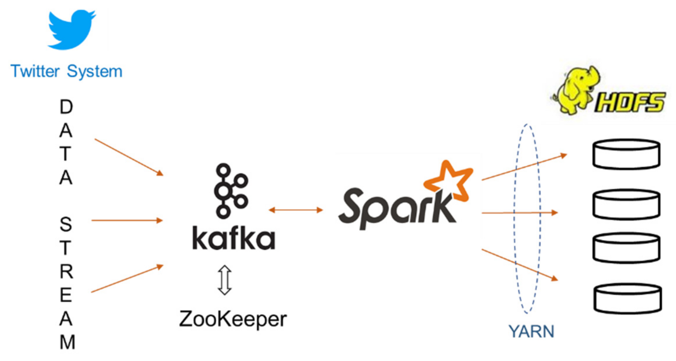
The algorithms to detect SIC, SC and SCIC from directed graphs in an Apache Spark framework using DataFrames, GraphX and GraphFrames API. As Spark provides data stream processing (using Spark Streaming as well as Kafka), the algorithms can potentially be used for analyzing the stream via the off-line computation approach for processing batches of data stream.

(3)

The use of motif finding in GraphFrames to discover temporal active communities. When the interaction patterns are known in advance, motif finding can be employed to find strongly connected component subgraphs. This process can be very efficient when the patterns are simple.

This paper is organized as follows: Section 2 discusses related work on community detection techniques as well as work that has been done in analyzing Twitter data and the big data technologies employed in this research, which are Spark, GraphX, and GraphFrames. Section 3 excerpts the results of the experiment comparing Strongly Connected Component algorithm and motif findings on Spark. Section 4 presents our proposed techniques. Section 5 discusses the experiments using public and Twitter data. In Section 6, we present our conclusions and further works.

2. Literature Review

2.1. Related Works

Formidably sized networks are becoming more and more common, such that many network sizes are expected to challenge the storage capability of a single physical computer. Fung [11] handles big networks with two approaches: first, he adopts big data technology and distributed computing as storage and processing, respectively. Second, he develops discrete mathematics in InfoMap for the distributed computing framework and then further develops the mathematics for a greedy algorithm, called InfoFlow, for detecting communities from undirected big graphs. InfoMap and InfoFlow are implemented on Apache Spark using the Scala language. The InfoFlow performance is evaluated using big graphs of 50,515 to 5,154,859 vertices and the results show that the runtime complexity of InfoFlow had logarithmic runtime complexity, while retaining accuracy in the resulted community.

The existing community detection algorithms principally propose iterative solutions of high polynomial order that repetitively require exhaustive analysis. These methods can undoubtedly be considered, resource-wise, to be overdemanding, unscalable, and inapplicable in big data graphs such as today’s social networks. To address these issues, Makris and Pispirigos [3] proposed a novel, near-linear, and scalable community prediction methodology. Using a distributed, stacking-based model, the underlined community hierarchy of any given social network is efficiently extracted in spite of its size and density. Their proposed method consists of three stages: first, subgraph extraction (the bootstrap resampling method is adopted and multiple BFS crawlers are randomly triggered to extract subgraphs of a predefined size; the maximum number of BFS crawlers, which are concurrently executed, is practically determined by the level of parallelism of the execution system); second, feature enrichment (each individual edge is properly enriched with features that include its network topology information up to a predefined depth of a value k; The value of k is an essential parameter that seriously affects the community prediction’s performance); third, a stacking ensemble learner is employed to detect communities (the independently trained, heterogeneous base learners are aptly combined by training a final model relying on the individual base learners’ predictions; it is built on top of a distributed bagging ensemble of L2 regularized, binary logistic regression classifiers, and a distributed gradient boosted trees ensemble model, also known as distributed GBT boosting ensemble model). To evaluate the methods, the experiments were conducted on Spark cluster with eight nodes using seven undirected and directed graphs (available at https://snap.stanford.edu/data/, accessed on 19 March 2021) having 1858 to 154,908 vertices. For evaluating the communities, the metrics measured are accuracy, recall, precision, specificity and F1-score. The metric values show that the models have detected the communities accordingly. The execution time of stacking ensemble methods executed in parallel on the Spark cluster beats that of the Louvain and Girwan–Newman methods that run on single node.

Bae et al. [1] developed a parallel algorithm for graph clustering called RelaxMap that parallelizes the optimization of flow-compression for community detection. It employs a prioritization strategy that avoids handling vertices that do not significantly improve the algorithm. The core algorithm works in two phases. In Phase 1, the visit probability (rank) of each vertex is computed in terms of the network flow. In Phase 2, tthe space of possible modularizations is greedily searched. In the search procedure for the best new module of a vertex v, the algorithm calculates the total in-flow and total out-flow between the vertex v and its neighbor modules (i.e., the set of modules to which any of its neighbors belong). The algorithm stops when the change in the minimum description length (MDL) score in each iteration is less than a minimum quality improvement threshold, Lprev − L < τ.

Bhatt et al. [12] proposed a community detection and characterization algorithm that incorporates the contextual information of node attributes described by multiple domain-specific hierarchical concept graphs. The core problem is to find the context that can best summarize the nodes in communities, while also discovering communities aligned with the context summarizing communities. The proposed algorithm iteratively optimizes two tasks, (i) optimal community label assignment while keeping the community context unchanged, and (ii) optimal community context assignment while keeping the community labels constant.

Most of the existing community detection methods have been proposed based exclusively on social connections. The emergence of geo-social networks (GeoSNs) motivates the integration of location information in community detection. In this context, a community contains a group of users that are tightly connected socially and are situated in the same geographic area. Yao, Papadias and Bakiras [4] have proposed a model called Density-based Geo-Community Detection (DGCD) in geo-social networks. This model extends the density-based clustering paradigm to consider both the spatial and social relationships between users. The results of the experiment show that the proposed model produces geo-social communities with strong social and spatial cohesiveness, which cannot be captured by existing graph or spatial clustering methods.

In [13], Jia et al. proposed CommunityGAN, a community detection framework that jointly solves overlapping community detection and graph representation learning. CommunityGAN aims to learn network embeddings like AGM (Affiliation Graph Model) through a specifically designed GAN. AGM is a framework which can model densely overlapping community structures. It assigns each vertex-community pair a nonnegative factor which represents the degree of membership of the vertex to the community. Thus, the strengths of membership from a vertex to all communities compose the representation vector of it. The algorithm of CommunityGAN takes as inputs the number of communities c, size of discriminating samples m, and size of generating samples n.

Roghani, Bouyer and Nourani [14] proposed a Spark-based parallel label diffusion and label selection-based (PLDLS) community detection algorithm using GraphX, which is an improved version of LPA, by putting aside randomness parameter tuning. PLDLS introduces NI, which is the importance measure of a node, used to find core nodes that initially form communities. For every node, NI(i) is locally computed using the following equation:

$$NI\left(i\right)=sim\_sum\left(i\right)\times \mathrm{deg}{\left(i\right)}^2$$

(1)

where $si{m}_{sum\left(i\right)}={\displaystyle \sum }_{j\in N_i}similarit{y}_{i,j}^{jaccard}$ and deg(i) is the degree measure of ith node.

In essence, PLDLS steps are as follows: Using GraphX, the input dataset is represented as an RDD containing pairs of vertex and edge collections, G(V,E). NI(i) is computed in parallel using Equation 1. Nodes having NI(i) ≥ Average (NI of all nodes) are selected. The modes of these selected nodes are computed. The communities are initialized with the member of core nodes with NI(i) ≥ mode of NI. The communities are then expanded by diffusing with their neighbors, to include first and second level nodes. First-level nodes are groups of neighbors (FLIN) that form a triangle with a core node and its most important neighbor; all of them at once get the same label. Second-level nodes are the neighbor nodes of FLIN that satisfy NI(FLIN) ≥ NI(i) and have Jaccard similarity higher than 0.5. Through iterative computation, the rest of the nodes (the unlabeled ones) are visited and labeled with their community ID. Using Pregel functions, the labels are improved, then the communities are merged in parallel (to integrate communities that are likely to be merged) in order to obtain more dense and accurate communities.

In real world networks, such as interpersonal relationship in human society and academic collaboration networks, communities tend to overlap. Thus, finding the overlapping community structure in complex networks is needed. As reported in [15], LinkSHRINK is an overlapping community detection method that combines density-based clustering with modularity optimization in a link graph. It finds overlapping communities by merging reductant nodes with parameter ω. It avoids the problem of excessive overlapping and reveals the overlapping community structure with different overlap degrees by using parameter ω. To find overlapping communities in large-scale networks, Zhang et al. [15] parallelized LinkSHRINK on Spark using GraphX (named as PLinkSHRINK) and Hadoop using Map-Reduce jobs (named as MLinkSHRINK). Through a series of experiments using synthetic and real networks, it is reported that: (1) while LinkSHRINK cannot handle very large graphs, PLinkSHRINK and MLinkSHRINK can find communities in large networks with millions of edges efficiently without losing significant accuracy; (2) on Spark, the running time of PLinkSHRINK correlates with the executer cores, or performance improves with an increasing number of cores; and (3) PLinkSHRINK runs faster on large networks than MLinkSHRINK and LinkSHRINK.

DENCAST [16] is a parallel clustering algorithm for Spark. It is based on a well-known density-based clustering algorithm, DBSCAN, which is able to identify arbitrarily shaped clusters. DBSCAN works iteratively and needs two parameters, which are eps (maximum distance of objects) and minPts (minimum points). DBSCAN starts with an arbitrary object o and, if this is a core object, it retrieves all the objects which are density-reachable from the core by using eps and minPts, and returns a cluster. The algorithm then proceeds with the next unclustered object until all objects are visited. Thus, DBSCAN works with graphs that represent the objects and their neighbors. Using GraphX on Spark, DENCAST identifies the reachable nodes of all the core objects simultaneously. This is performed by propagating the cluster assignment of all the core objects to their neighbors until the cluster assignment appears stable enough. Based on the evaluation experiments on a Spark cluster, it was concluded that DENCAST is able to handle large-scale and high-dimensional data. The model has high accuracy. It also significantly outperforms the distributed version of K-means in Apache Spark in terms of running times.

In [17], Krishna and Sharma discuss the review results of five parallel community detection algorithms, as follows: (1) the distributed memory-based parallel algorithm based on modularity maximization proposed by Louvain and implemented on an MPI-based HPC cluster; (2) Picaso, a parallel community detection model based on approximate optimization. It is based on two approaches: a computing “mountain” (of vertices) based on approximate optimization and modularity, and the Landslide algorithm, which is iterative and implemented using GraphX on Spark; (3) FPMQA, a parallel modularity optimization algorithm that uses the modularity technique to identify communities in the social networks. The networks are initialized with people connected based on their comments on similar topic of interests, namely similar view network (SVN). The FPMQA algorithm is executed in parallel to process this SVN (there will be a group of nodes connected in this SVN due to common interest). Based on gain modularity measures, SVNs may be merged. The modularity computation is done in parallel; (4) PLPAC, a label propagation-based parallel community detection algorithm with nodes confidence. In label propagation algorithm (LPA), each node label (denoting its community ID) is updated based on the labels with the highest modularity among their neighbors. The proposed parallel algorithm is implemented using MapReduce; (5) an algorithm for detecting disjointed communities on large-scale networks, which is based on the Louvain algorithm and implemented for parallel shared memory. All of the algorithms discussed in [17] work with undirected graphs, or do not consider direction (of the edges between nodes) as important for finding communities.

Atastina et al. [7] discusses how to process communication transaction data to find the communities and track the evolution of the communities over time. The Facetnet algorithm, which is based on clustering vertices, is applied to undirected graphs to mine the communities.

Twitter messages or tweets, which originate from all over the world using many languages, have also attracted researchers. Three examples of recent work results are excerpted below.

In a case study using Twitter data, Sadri et al. [18] analyzed the characteristics and growth of online social interaction networks, examining the network properties and deriving important insights based on the theories of network science literature. The data is specific to the Purdue University community. They collected tweets (between 16 April 2016 and 16 May 2016) using a specific keyword ‘purdue’ and captured 56,159 tweets. Of these tweets, 19,532 did not include any user mentions, while the rest of the tweets included at least one user mention in each tweet. The dataset contains 34,363 unique users and 38,442 unique undirected links (39,709 links if direction is considered). The graphs, which are created from users and their mentions, are analyzed as both undirected and directed graphs, using visualization, vertex degree (including in-out degree), graph radius, connected component and clustering. Key insights found were: (i) the graph indicated that with some vertices being highly active, there are connected components and hubs; (ii) network elements and average user degree grow linearly each day, but network densities tend to become zero, and the largest connected components exhibit higher connectivity when compared to the whole graph; (iii) network radius and diameter become stable over time, which suggests a small-world property.

All of the above community detection techniques do not discuss the importance of edge direction. The directed graphs discussed in [18] are only used to compute in-out degree.

2.2. Spark, GraphX and GraphFrames

2.2.1. Apache Spark

Apache Spark is a data processing framework that is fast and scalable for processing big data, employing non-iterative as well as iterative algorithms. It is written in Scala and runs in Java Virtual Machine (JVM). For processing big data, Spark is more often used in tandem with a distributed storage system (such as Hadoop Distributed File System, HDFS) and a cluster manager, such as Apache Hadoop YARN [6,19,20]. HDFS is a distributed file system designed to reliably store very large files across machines in a large cluster. Each HDFS file is stored as a sequence of blocks; these blocks are replicated for fault tolerance. Apache Hadoop YARN (Yet Another Resource Negotiator) provides the resource management and job scheduling for Hadoop clusters, consisting of master and data (slave/worker) nodes [21,22]. As YARN is able to manage clusters each with thousands of machines, it supports Spark scalability for processing big data. When run on top of YARN, a physical Spark cluster that consists of driver and worker machines may have thousands of workers that can run parallel tasks on the workers.

Resilient Distributed Datasets. Spark is built around a data abstraction called Resilient Distributed Datasets (RDD). An RDD is an immutable distributed collection of objects and is commonly split into multiple partitions [19,23]. Those partitions are stored across worker nodes’ memory if Spark is run on YARN or another resource manager. Each partition of an RDD can be processed by one task or more that run parallel across the core machines, which speeds up overall computation. Once created, RDDs offer two types of operations, transformations and actions. Actions are functions that return values that are not RDDs, whereas transformations return other forms of RDD. Each Spark application must contain at least one action (such as collect, count, take and saveAsTextFile), since actions either bring information back to the driver or write the data to stable storage. Transformations (such as sort, reduce, group and filter) construct new RDDs from the old ones. Transformations and actions are different because of the way Spark computes RDDs. Operations on RDDs are queued up in a lazy fashion and then executed all at once only when needed, that is, when an action is called. At this time, Spark optimizes those operations and also plans data shuffles (which involve expensive communication, serialization, and disk I/O) and generates an execution graph, the Directed Acyclic Graph (DAG), detailing a series of execution plans; it then executes these plans [5]. Spark can keep an RDD loaded in-memory on the executor nodes throughout the life of a Spark application for faster access in repeated computations [21].

Spark Application. A Spark application corresponds to a set of Spark jobs defined by one SparkContext in the driver program [4]. A Spark application begins when a SparkContext is started, which causes a driver and a series of executors be started on the worker nodes of the cluster. Each executor corresponds to a JVM. The SparkContext determines how many resources are allotted to each executor. When a Spark job is launched, each executor has slots for running the tasks needed to compute an RDD. Physically, each task runs on a machine core, and one task may process one or more RDD partition (when an RDD is created by loading a HDFS file, the default is: Spark creates an RDD partition for each HDFS block, and stores this partition in the memory of the machine that has the block). One Spark cluster can run several Spark applications concurrently. The applications are scheduled by the cluster manager and correspond to one SparkContext.

A Spark application can run multiple concurrent jobs, whereas a job corresponds to an RDD action that is called (see Figure 1). That is, when an RDD action is called, the Spark scheduler builds a DAG and launches a job. Each job consists of stages. One stage corresponds to one wide-transformation, which occurs when a reducer function that triggers shuffling data (stored as RDD partitions) across the network is called (see Figure 2). Each stage consists of tasks, which are run in parallel, and each task executes the same instruction on an executor [19,23]. The number of tasks per stage depends on the number of RDD partitions and the outputs of the computations.

Examples of transformations that cause shuffling include groupByKey, reduceByKey, aggregateByKey, sortByKey, and join. Several narrow transformations (such as map, filter, mapPartitions and sample) are grouped into one stage. As shuffling is known as an expensive operation and can degrade computation, it is necessary to design Spark applications that involve minimum number of shuffles or stages to achieve better performance.

2.2.2. GraphX and GraphFrames

GraphX is an embedded graph processing framework built on top of Apache Spark. It implements a notion called the property graph, whereby both vertices and edges can have arbitrary sets of attributes associated with them. GraphX recasts graph-specific optimizations as distributed join optimizations and materialized view maintenance [24]. Users can simply use GraphX’s API to operate on those graph data structures [5]. This provides a powerful low-level interface. However, like RDDs it is not easy to use or optimize. However, GraphX remains a core part of Spark for graph processing [6].

Distributed Graph Representation [24]: GraphX represents graphs internally as a pair of vertex and edge collections built on the RDD abstraction. These collections introduce indexing and graph-specific partitioning as a layer on top of RDDs. The vertex collection is hash-partitioned by the vertex IDs. To support frequent joins across vertex collections, vertices are stored in a local hash index within each partition. The edge collection is horizontally partitioned. GraphX enables vertex-cut partitioning. By default, edges are assigned to partitions based on the partitioning of the input collection (e.g., the HDFS blocks). A key stage in graph computation is constructing and maintaining the triplets view, which consists of a three-way join between the source and destination vertex properties and the edge properties. The techniques used include Vertex Mirroring, Multicast Join, Partial Materialization, and Incremental View Maintenance.

GraphX API provides an implemented standard algorithm, such as PageRank, Connected Components and Strongly Connected Components (SCC). While the Connected Components algorithm is relevant for both directed and undirected graphs, Strongly Connected Components is for directed graphs only, and can be used to detect vertices that have “reciprocated connections”. A few of the graph algorithms, such as SCC, are implemented using Pregel.

The Pregel algorithm that computes SCCs from a directed graph G = (V,E) is excerpted as follows.

Let SCC(v) be the SCC that contains v, and let Out(v) (and In(v)) be the set of vertices that can be reached from v (and that can reach v) in G, then SCC(v) = Out(v) ∩ In(v). Out(v) and In(v) are computed by forward/backward breadth-first search (BFS) from a source v that is randomly picked from G. This process then repeats on G[Out(v) − SCC(v)], G[In(v) − SCC(v)] and G[V − (Out(v)ՍIn(v) − SCC(v))], where G[X] denotes the subgraph of G induced by vertex set X. The correctness is guaranteed by the property that any remaining SCC must be in one of these subgraphs.

Yan et al. [25] designed two Pregel algorithms based on label propagation. The first propagates the smallest vertex (ID) that every vertex has seen so far (namely, the miLabel algorithm), while the second propagates multiple source vertices to speed up SCC computation (namely, multi-Label algorithm). miLabel algorithm requires a graph decomposition, which allows the algorithm to run multiple rounds of label propagation.

Graph Decomposition: given a partition V, denoted by V₁, V₂, …, V_l, G is decomposed into G[V₁], G[V₂], …, G[V_l] in two supersets (here, each vertex v contains a label i indicating v ε V_i): (i) each vertex notifies all its in-neighbors and out-neighbors about its label i; (ii) each vertex checks the incoming messages, removes the edges from/to the vertices having labels different from its own label, and votes to halt.

MinLabel Algorithm: the min-label algorithm repeats the following operations: (i) forward min-label propagation; (ii) backward min-label propagation; (iii) an aggregator collects label pairs (i, j), and assigns a unique ID to each V_(i,j); graph decomposition is then performed to remove edges crossing different G[V_ID]; finally, each vertex v is labeled with (i; i) to indicate that its SCC is found. In each step, only unmarked vertices are active, and thus vertices do not participate in later rounds once their SCC is determined. Each round of the algorithm refines the vertex partition of the previous round. The algorithm terminates once all vertices are marked.

GraphX Weaknesses: GraphX limitations stem from the limitations of Spark. GraphX is limited by the immutability of RDDs, which is an issue for large graphs [5]. In some cases, it also suffers from a number of significant performance problems [21].

GraphFrames extends GraphX to provide a DataFrame API and support for Spark’s different language bindings so that users of Python can take advantage of the scalability of the tool [6]. So far, it is a better alternative to GraphX [21]. GraphFrames is an integrated system that lets Spark users combine graph algorithms, pattern matching and relational queries, and optimizes work across them. A GraphFrame is logically represented as two DataFrames: an edge DataFrame and a vertex DataFrame [8].

In Spark, DataFrames are distributed as table-like collections with well-defined rows and columns [6]. These consist of a series of records that are of type Row, and a number of columns that represent a computation expression that can be performed on each individual record in the Dataset. Schemas define the name as well as the type of data in each column. Spark manipulates Row objects using column expressions in order to produce usable values. Filtering and applying aggregate functions (count, sum, average, etc.) to group records are among these useful expressions. With its lazy computation (see Section 2.2.1), whenever Spark receives a series of expressions for manipulating DataFrames that need to return values, it analyzes those expressions, prepares a logical optimized execution plan, creates a physical plan, then executes the plan by coordinating with the resource manager (such as YARN) to generate parallel tasks among the workers in the Spark cluster.

GraphFrames generalizes the ideas in previous graph-on-RDBMS systems, by letting the system materialize multiple views of the graph and executing both iterative algorithms and pattern matching using joins [8]. It provides a pattern operator that enables easy expression of pattern matching in graphs. Typical graph patterns consist of two nodes connected by a directed edge relationship, which is represented in the format ()-[]->(). The graph patterns as the input of the pattern operator are usually called network motifs, which are sub-graphs that repeat themselves in the graph that is analyzed. The pattern operator is a simple and intuitive way to specify pattern matching. Under the hood, it is implemented using the join and filter operators available on a GraphFrame.

Because GraphFrames builds on top of Spark, this brings three benefits: (i) GraphFrames can load data from the volumes saved data in many formats supported by Spark (GraphFrames has the capability of processing graphs having millions or even billions of vertices and edges); (ii) GraphFrames can use a growing list of machine learning algorithms in MLlib; and (iii) GraphFrames can call the Spark DataFrame API.

One case of using GraphFrames is discussed in [26], where an efficient method of processing SPARQL queries over GraphFrames was proposed. The queries were applied to graph data in the form of a Resource Description Framework (RDF) that was used to model information in the form of triples <subject, predicate, object>, where each edge can be stored as a triple. They created queries based on two types of SPARQL queries, chain queries and star-join queries. The experiments were performed using the dataset produced by the Lehigh University benchmark (LUBM) data generator, which is a synthetic OWL (Web Ontology Language) dataset for a university. Overall, the proposed approach works well for large datasets.

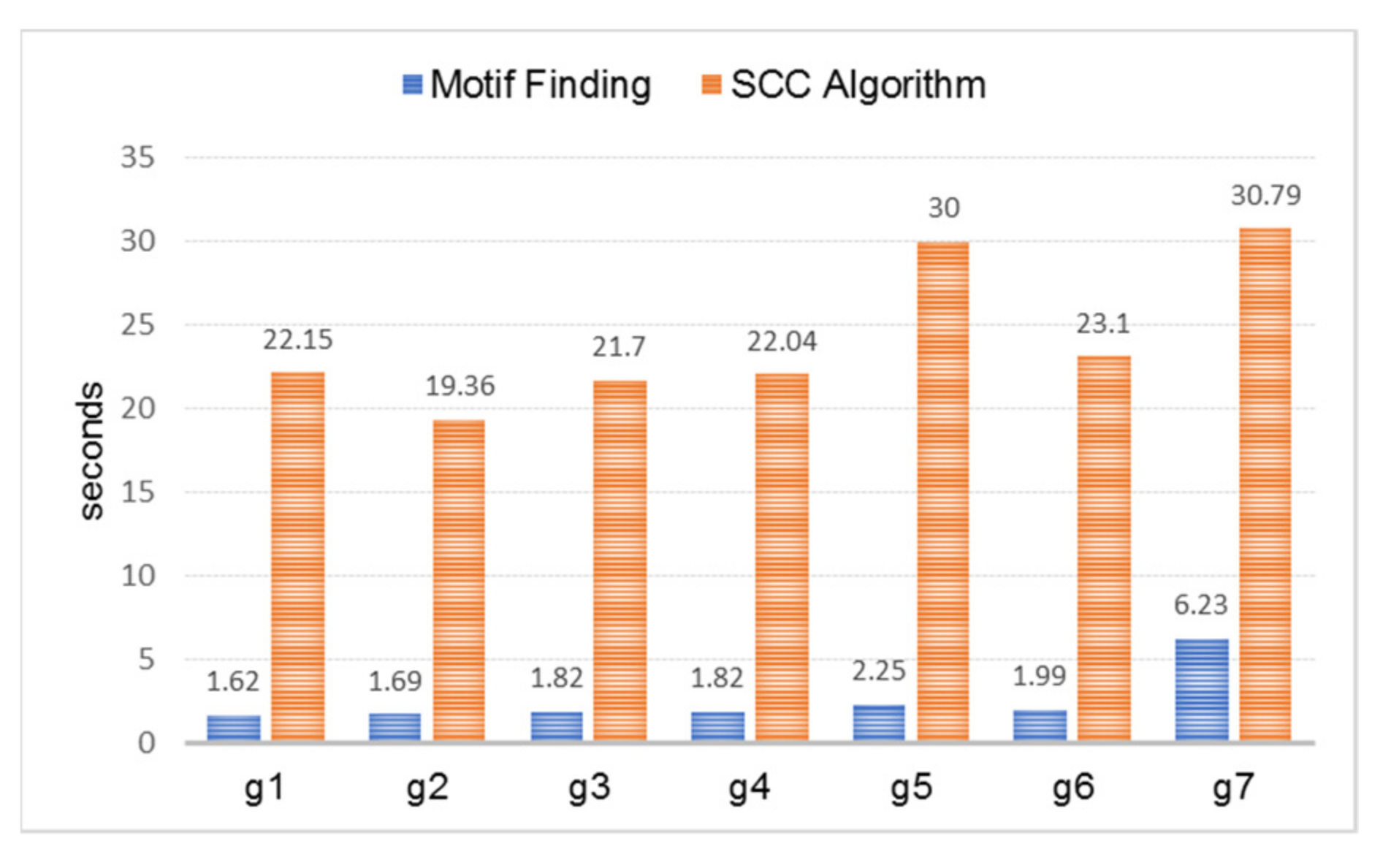
3. Comparing SCC Algorithm and Motif Finding on Spark

As presented in Section 2.2.2, GraphFrames provides graph pattern matching (motif finding). We found that SCC subgraphs used to uncover active communities from directed graphs can be detected using GraphX SCC algorithm as well motif finding. In this section, we present our experimental results of SCC algorithm and motif finding performance.

As discussed in Section 2.2.1, data shuffling across a Spark cluster is expensive. When an algorithm for processing big data is run, Spark generates a stage whenever it encounters a wide transformation function, a computation that requires shuffling among RDD partitions across the network. Using the Spark web UI, we can observe and learn several kinds of computation statistics, DAG, execution plan and other related information regarding the applications being run. The DAG, execution plan, jobs, stages and parallel tasks can be used to measure the complexity of the program or algorithm that is run.

We created seven synthetic small graph datasets (g1, g2, …, g7), each consisting of vertex and edge dataframes. Each of the six datasets has an SCC subgraph that is shown in Figure 3, while one dataset (g7) contains all of the SCC subgraphs.

As the synthetic datasets are small, we performed these experiments on a Spark cluster with a single machine with i7-3770 CPU, four cores and 16 Gb memory. The cluster ran Apache Spark 2.4.5, Java 1.8.0_40, and Scala 2.11.12. The following steps were performed for each graph dataset:

(1)

An instance of GraphFrame for each graph dataset was created;

(2)

SCC algorithm was used to detect SCCs from the graph instance;

(3)

A set of patterns was searched from the graph instance. The pattern set searched on g1 was “(a)-[e1]->(b); (b)-[e2]->(a)”, g2 was “(a)-[e1]->(b); (b)-[e2]->(c); (c)-[e3]->(a)”, g3 was “(a)-[e1]->(b); (b)-[e2]->(c); (c)-[e3]->(d); (d)-[e4]->(a)”, g4 was “(a)-[e1]->(b); (b)-[e2]->(c); (c)-[e3]->(b); (b)-[e4]->(a)”, g5 was “(a)-[e1]->(b); (b)-[e2]->(c); (c)-[e3]->(d); (d)-[e4]->(e); (e)-[e5]->(a)”, and g6 was “(a)-[e1]->(b); (b)-[e2]->(c); (c)-[e3]->(b); (b)-[e4]->(a);(c)-[e5]->(d); (d)-[e6]->(c)”. For g7, all of the patterns were combined.

Then the execution time as well as the information on the Spark web UI were observed on each run and recorded.

The Scala codes executed in these experiments are attached in Appendix A.

As discussed in Section 2.2.2, motif findings were executed using the join and filter operators. For instance, below is the optimized logical plan of query (a), g1.find(“(a)-[e1]->(b); (b)-[e2]->(a)”) generated by Spark:

1   +- Project [cast(a#34 as string) AS a#83, cast(e1#32 as string)

             AS e1#84, cast(b#36 as string) AS b#85, cast(e2#57 as string)

               AS e2#86]

2      +- Join Inner, ((e2#57.src = b#36.id) && (e2#57.dst = a#34.id))

3         : - Join Inner, (e1#32.dst = b#36.id)

4         :  : - Join Inner, (e1#32.src = a#34.id)

5         :  :  : - Project [named_struct(src, src#10, dst, dst#11, weight, weight#12) AS e1#32]

6         :  :  :  +- Relation[src#10,dst#11,weight#12] csv

7         :  :  +- Project [named_struct(id, id#26) AS a#34]

8         :  :  +- Relation[id#26] csv

9         :  +- Project [named_struct(id, id#26) AS b#36]

10         :     +- Relation[id#26] csv

11         + - Project [named_struct(src, src#10, dst, dst#11, weight, weight#12) AS e2#57]

12            +- Relation[src#10,dst#11,weight#12] csv

In the plan above, the inner join (between vertex and edge dataframes) is performed three times, to resolve part of the query “(a)-[e1]” (line 4), “(a)-[e1]->(b)” (line 3) and “(b)-[e2]->(a)” (line 2). As discussed in Section 2.2.1, a Spark job is created when an application calls an RDD action. Here, a job is created each time a project (filter) operation is applied to the result of the join (line 5, 7, 9, and 11). Thus, there are four jobs. The overall DAG is shown on Figure 4. In the physical execution plan, the inner join is implemented by BroadcastExchange then BroadcastHashJoin. Broadcasting records stored in the RDD partitions causes data shuffling (such as in wide transformation) that produces one stage. Hence, there are four stages (one job only having one stage). Other queries of motif findings are executed using join and filter, analogous to (a); the number of jobs and stages is presented on

Table 1. Comparison of Spark jobs and stages.

Case	Graph	Motif Finding		SCC Algorithm
		#Jobs	#Stages	#Jobs	#Stages
(a)	g1	4	4	29	75
(b)	g2	6	6	28	75
(c)	g3	8	8	30	83
(d)	g4	7	7	32	80
(e)	g5	10	10	38	105
(f)	g6	10	10	37	98
(g)	g7	45	45	41	114

.

Unlike motif findings, which implement queries where the execution plan is available for observation, when running the SCC algorithm (as with other algorithms designed based on RDD) we can only observe the execution process through its jobs, stages, DAG and tasks. As can be observed, when the SCC algorithm is run it requires many jobs and stages (see Table 1). For instance, when processing g1, Spark generates 29 jobs. As an example, the DAG of its sixth job (with Id 9) with three stages is provided in Appendix A, Figure A1: Stage 14 performs mapping at GraphFrame, Stage 13 performs mapPartitioning at VertexRDD, and Stage 15 folding at VertexRDDImpl. From the number of jobs, stages and DAG, we can learn that the implementation of the iterative SCC algorithm on Spark (see Section 2.2.2) is complex and requires lots of machine and network resources.

In line with the number of jobs and stages (Table 1), the execution time of each motif finding is also smaller compared to the SCC algorithm (see Figure 5).

It is known that hash-join time complexity is O(n + m), where n + m denotes the total records in two tables being joined. On a system with p cores, the expected complexity of the parallel version of no partitioning hash join is O((n + m)/p) [27]. Although this complexity it not specifically applied for hash join in Spark, the motif finding execution time seems to be in line with O((n + m)/p).

The time complexity of parallel SCC algorithm for Spark is not discussed in [8] and [24]. To the best of our knowledge, it is not discussed in any other literature either. However, by comparing the stages of SCC versus motif finding presented in Table 1, it can be learned that the SCC computation is far more complex than the motif finding.

Findings of these experiments: when there are not many patterns of SCC subgraphs in a directed graph, motif finding runs faster and uses less network resources compared to the SCC algorithm. Hence, this can be used as an optional technique in finding active communities from directed graphs.

4. Proposed Techniques

A streaming computational model is one of the widely used models for processing and analyzing massive data [9]. Based on the methodology for processing data streams, a data stream can be classified as an online (live stream) data stream or an off-line (archived) data stream. Online data streams (such as those of stock tickers, network measurements, and sensor data) need to be processed online because of their high speed. An Off-line stream is a sequence of updates to warehouses or backup devices, where the queries over the off-line stream can be processed offline. The online method is constrained by the detection and reaction times due to the requirement of real-time applications, while the off-line is free from this requirement. Depending on its objective (such as finding trending topics vs. detecting communities), a stream of tweets can be processed either online or off-line. We proposed techniques that can be used to analyze off-line as well as near-real-time batches of data stream to uncover temporal active communities using the SCC algorithm and motif finding in Spark.

4.1. Active Communities Definition

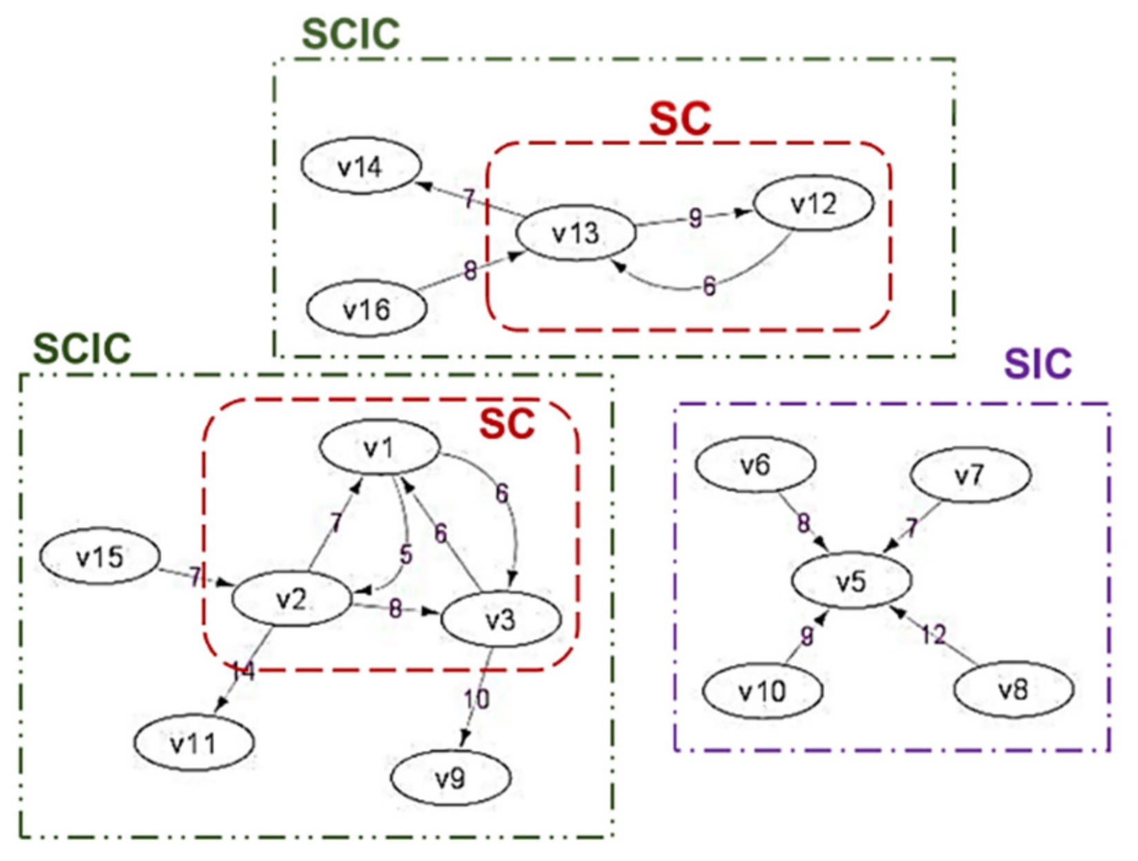
Based on our observation of Twitter users’ posts, we learned that during certain periods of time (such as weekly) lots of users either send tweets or respond to other users’ tweets in ways that show patterns. Only tweets that draw other users’ interest were responded to with retweet, reply or quote tweets. Thus, based on their interests that lead to frequent responses, Twitter users may form temporal active communities without intent. To form graphs that can be used to uncover these communities, the Twitter users are defined as vertices, while their interactions (reply and quote) become the edges. The number of interactions can be included as an edge attribute (such as weight), which then may be used to select the frequent vertices (vertices who communicate to each other frequently) by applying a threshold value.

For a certain (relatively short) period of time, we define three types of active communities (see Figure 6):

(1)

Similar interest communities (SIC): A group of people responding to the same event. Real world examples: (a) Twitter users who frequently retweet or reply or quote a user’s tweets, which means that those users have the same interest toward the tweet content; (b) forum users who frequently give comments or reply to posts/threads posted by certain user/users, which means those users have the same interest in discussion subjects.

(2)

Strong-interacting communities (SC): A group of people who interact with each other frequently in a period of time. Real world example: a group of people who reply/call/email/tweet/message each other.

(3)

Strong-interacting communities with their “inner circle” neighbors (SCIC): The extension of SC, where SC members become the core of the communities, added by the “external” people who are frequently directly contacted by the core members, as well as “external” people who directly contact the core members. Real world example: as in the aforementioned SC, now also including the surrounding people who actively communicate with them.

4.2. Proposed Algorithms

Based on the previous definition, we propose three techniques to process weighted directed graphs, G. G = (V,E) where V = vertices, E = edges. E must have one or more attributes, including its weight. V may have one attribute or more, thus E(Id, at₁, at₂, …), where Id is the Id of the vertex, followed by its attributes. E(srcId, dstId, a₁, a₂, …, w), where srcId = Id of the source vertex, dstId = Id of the target vertex, a_i = i-th attribute, w = weight of edges, denoting the count of srcId interacts to dstId.

(a)

Detecting SIC from directed graphs

The proposed algorithm (Algorithm 1) is simple, in that it is only based on dataframe queries.

Algorithm 1: DetectSIC

Descriptions: Detecting SIC from a directed graph using GraphFrame Input: Directed graph G, thWC1 = threshold of w; thIndeg = threshold of vertices in-degree Output: Communities stored in map structure, comSIC = map(CenterId, list of member Ids); a vertex can be member of more than one community. Steps: (1) Graph preparation: (a) filteredE = E in G with w > thWC1 //Only edges having w > thWC1 is used to construct the graph; (b) GFil = (V, filteredE) (2) Compute inDeg for every vertex in GFil, store into dataframe, inD(Id, inDegree) (3) selInD (IdF, inDegree) = inD where inDeg > thIndeg (4) Find communities: (a) dfCom = (GFil where its nodes having Id = selInD.IdF) inner join with E on Id = dstId, order by Id; (b) Collect partitions of dfCom from every worker (coalesce) then iterate on each record: read Id and srcId column, map the pair value of (Id, srcId) into comSIC

(b)

Detecting SC using motif finding

In this proposed algorithm (Algorithm 2), the data preparation is performed for reducing the number of vertices in the graphs. Only vertices passing the filter with a threshold of degree that will be further processed. In this algorithm, strongly connected sub-graphs, which are further processed into communities, are detected using motif findings described in Section 2.2 and Section 3.

Algorithm 2: DetectSC-with-MotifFinding

Descriptions: Detecting SC using motif finding Input: Directed graph G; thWC1 = threshold of w; thDeg = threshold of vertices degree; motifs = {motif1, motif2, …, motifn} where motif1 = 1st pattern of SC, motif2 = 2nd pattern of SC, motifn = the nth pattern of SC Output: Communities stored in map structure, comSCMotif = map(member_Ids: String, member_count: Int) where member_Ids contains list of Id. A vertex can be member of more than one community. Steps: (1) Graph preparation: (a) filteredE = E in G with w > thWC1; (b) GFil = (V, filteredE) (2) Compute degrees for every vertex in GFil, store into a dataframe, deg(Id, degree) (3) selDeg (IdF, degree) = deg where degree > thDeg (4) Gsel = subgraph of GFil where its nodes having Id = selInD.IdF (5) For each motifi in motifs, execute Gsel.find(motifi), store the results in dfMi, filter records in dfMi to discard repetitive set of nodes (6) Collect partitions of dfMi from every worker (coalesce), then call findComDFM(dfMi)

In step 5: As motif finding computes the SC using repetitive inner join (of node Ids), a set of Ids (for an SC) exists in more than one record. For an SC with n member, the set will appear in n! records. For instance, an SC with vertex Id {Id1, Id2, Id3} will appear in six records, where the attributes of the nodes are in the order of {Id1, Id2, Id3}, {Id1, Id3, Id2}, {Id2, Id1, Id3}, {Id2, Id3, Id1}, {Id3, Id1, Id2} and {Id3, Id2, Id1}. Thus, only one record must be kept by filtering them.

In step 6: The size of dfM_i, where its partitions are stored in the workers, generally will be a lot smaller than G, therefore this dataframe can be collected into the master and computed locally using non-parallel computation (Algorithm 3).

Algorithm 3: findComDFM

Descriptions: Formatting communities from dataframe dfMi Input: dfMi Output: Communities stored in map structure, comSCMotif: map(member_Ids: String, member_count: Int). member_Ids: string of sorted Ids (separated by space) in a community, member_count: count of Ids in a community Steps: (1) For each row in collected dfMi: (2)    line = row (3)    parse line and find every vertex Id in str with space to separate between Id,           with the count of Ids store in member_count (4)    sort Ids in str in ascending order (5)    add (str, Id) into comMotif // as str is the key in comMotif, only unique value of str will be successfully added

(c)

Detecting SC using SCC algorithm

Given the complexity of the SCC algorithm computation (see Section 2.2.2), the number of vertices in the graph will be reduced by filtering those having a threshold of degree. The SCC algorithm in Spark returns a dataframe of sccs(Id, IdCom), where Id is a vertex Id and IdCom is the Id of the connected component where that vertex is being grouped. Thus, for obtaining the final SC, that dataframe is further processed in Algorithm 4 that calls Algorithm 5 on Step 6.

Algorithm 4: DetectSC-with-SCC

Descriptions: Detecting SC using SCC algorithm Input: Directed graph G; thWC1 = threshold of w; thDeg = threshold of vertices degree; thCtMember = threshold of member counts in an SCC Output: Communities stored in map structure, comSIC = map(CenterId, list of member Ids). A vertex can be member of more than one community. Steps: (1) Graph preparation: (a) filteredE = E in G with w > thWC1; (b) GFil = (V, filteredE) (2) filteredG = subgraph of GFil where each vertex has degree > thDeg (3) Find strongly connected components from filteredG, store as sccs dataframe (4) Using group by, create dataframe dfCt(idCom,count), then filter with count > thCtMember // The SCC algorithm record every vertex as a member of an SCC (SCC may contain one vertex only) (5) Join sccs and dfCt on Id = IdCom store into sccsSel // sccsSel contains only records in a community having more than one member (6) Collect partitions of sccsSel from every worker, sort the records by idCom in ascending order, then call findComSC(sccsSel)

Algorithm 5: findComSC

Descriptions: Formatting communities from sccsSel Input: Dataframe containing connected vertices, sccs(id, idCom) Output: Communities stored in map structure, comSCC: map(idCom: String, ids_count: String). idCom: string of community Id, Ids_count: strings of list of vertex Ids in a community separated by space and count of Ids. Steps: (1) prevIdCom = “”; keyStr = “”; addStatus = false; nMember = 0 (2) For each row in sccsSel (3)   line = row; parse line; strId = line[0]; idC = line[1] (4)   if line is the first line: add strId to keyStr; prevIdCom = idC;         nMember = nMember + 1 (5)   else if prevIdCom == idC and line is not the last line: add strId to keyStr;         nMember = nMember + 1 (6)   else if prevIdCom != idC and line is not the last line: add strId  to keyStr,            nMember = nMember + 1; add (keyStr, nMember) to comSCC; keyStr =””; nMember = 0; addStatus = true;    //Final check (7)   if addStatus == false and line is the last line: add (keyStr, nMember) to comSCC; addStatus = true;

(d)

Detecting SCIC

The members in an SCIC are the vertices in SCC and the neighbor vertices (connected to the vertices in a SCC by “in-bound” or “out-bound” connection). After the dataframe containing the SCC vertices is computed using Algorithm 4, the steps in Algorithm 6 are added with dataframe join operations. On Step 10, Algorithm 7 is called to format the communities. In Algorithm 8, steps of Algorithm 2 are added with more steps to process the SCC neighboors vertices as well.

Algorithm 6: DetectSCIC-with-SCC

Descriptions: Detecting SCIC using SCC algorithm Input: Directed graph G; thWC1 = threshold of w; thDeg = threshold of vertices degree; thCtMember = threshold of member counts in an SCC Output: Communities stored in map structure, comSCIC = map(idCom: String, ids_count: String). A vertex can be member of more than one community. Steps: Step 1 to 6 is the same with the ones in DetectSC-with-SCC. (7) Join sccsSel with filteredE based on sccsSel.id = filteredE.dst store as dfIntoSCC with src column renamed as friendId //neighbor nodes contact SCC nodes (8) Join sccsSel with filteredE based on sccsSel.id = filteredE.src store as dfFromSCC with dst column renamed as friendId // neighbor nodes contacted by SCC nodes (9) Merge dfIntoSCC and dfFromSCC into dfComExpand dataframe using union operation (10) Collect partitions of dfComExpand from every worker, sort the records by IdCom in ascending order, then call findComSCIC(dfComExpand) // The schema is: dfComExpand(id, idCom, friendId)

Algorithm 7: findComSCIC

Descriptions: Formatting communities from dfComExpand Input: Dataframe containing connected vertices, dfComExpand (id, idCom, friendId ) Output: Communities stored in map structure, comSCIC: map(idCom: String, ids_count: String). idCom: string of community Id, Ids_count: strings of vertex Ids in a community separated by space and count of Ids the community. Steps: (1) prevIdCom = “”; keyStr = “”; addStatus = false; nMember = 0 (2) For each row in dfComExpand (3)    line = row; parse line; strId = line[0]; idC = line[1]; idFr = line[2] (4)    if line is the first line: add strId and idFr to keyStr; prevIdCom = idC;          nMember = nMember + 2 (5)   else if prevIdCom == idC and line is not the last line: add idFr to keyStr;          nMember = nMember + 1 (6)   else if prevIdCom != idC and line is not the last line: add idFr to keyStr,          nMember = nMember + 1; add (keyStr, nMember) to comSCC;          keyStr =””; nMember = 0; addStatus = true;    //Final check (7)  if addStatus == false and line is the last line: add (keyStr, nMember) to comSCC; addStatus = true;

Algorithm 8: DetectSCIC-with-Motif

Descriptions: Detecting SCIC using motif finding Input: Directed graph G; thWC1 = threshold of w; thDeg = threshold of vertices degree; thCtMember = threshold of member counts in an SCC Output: Communities stored in map structure, comSCICMotif = map(IdCom, list of member Ids). A vertex can be member of more than one community. Steps: Step 1 to 6 is the same with the ones in DetectSC-with- Motif (7) Initialize an array, arrCom(IdCom, IdM) where IdCom is Id of the community, IdM is Id of the member; IdC = 0 (8) for each pair of (member_Ids, member_count) from comSCMotif: (9)       IdC = IdC + 1 (10)       parse member_Ids then for each Id add(IdC, Id) into arrCom (11) create a dataframe, dfCom(IdCom, id) from arrCom (12) Join dfCom with filteredE based on dfCom.id = filteredE.dst store as dfIntoSCC with src column renamed as friendId //neighbor nodes contact SCC nodes (13) Join dfCom with filteredE based on dfCom.id = filteredE.src store as dfFromSCC with dst column renamed as friendId // neighbor nodes contacted by SCC nodes (14) Merge dfIntoSCC and dfFromSCC into dfComExpand dataframe using union operation (15) Collect partitions of dfComExpand from every worker, sort the records by IdCom in ascending order, then call findComSCIC(dfComExpand) // The schema is: dfComExpand(id, idCom, friendId)

5. Experiments and Results

In this section, we present some results of the experiments of our proposed methods. All of the experiments discussed below were conducted on a Spark cluster, which is physically located in our laboratories. It consists of ten machines (one as a driver and nine as workers), each with CPU i7-9700K running at 3.6 GHz and has eight cores, with RAM of 32 Gb. The cluster ran Apache Spark 2.4.5, Java 1.8.0_292, Hadoop 3.1.3 with YARN and Scala 2.11.12. While performing the experiments, we used nine workers, each with four cores.

5.1. Public Big Graphs

To obtain the data, we looked for suitable examples from large network datasets, which are available at https://snap.stanford.edu/data/ (accessed on 19 March 2021) There are many groups of datasets, such as social, citation, road, Amazon, online reviews, etc. The graph types are also categorized into undirected and directed. Among those datasets, we identified the ones that are directed and can be preprocessed (by aggregating the vertex interaction count then adding weight on the edges) such that there was a possibility that active communities could be uncovered from those datasets. Among those datasets we found only two, both of which consist of social circles: Google+ [28] and Twitter.

The first, the social circle dataset from Google+, ego-Gplus, is a directed graph dataset with 107,614 nodes and 13,673,453 edges. After a dataframe was created and the weight of edges (denoting the number of interactions between nodes) is aggregated, the distribution (range of weight:count) were as follows: 1–9: 13,291,770; 10–18: 319,710; 19–27: 48,409; 28–36: 11,413; 37–70: 2151. The average weight was 2.23, the minimum weight 1, and the maximum weight 70. Since there was no information on how long the data were recorded for (which would determine the weight threshold), we used a threshold of weight based on that distribution, (thW) = 9. Thus, only edges (with nodes connected with these edges) having weight = 10 and more were selected. After filtering the edges using this threshold, there were 381,683 edges passing this filter, with 515,322 vertices connected by those edges.

Given the large size of the graphs, the visualization of the graphs did not clearly show the patterns of SCCs. Therefore, discovering SCIC was performed using Algorithm 6. Algorithm 6 was run by varying the value of thDeg and thCtMember from 2 to 10. By using this algorithm, we only discovered two SCICs with unbalanced members. The first community had a very large number of members (such as 515,041) while the second had only a small number of members (such as 75). As each community had only member IDs, we could not interpret the pattern of the communities. If the time of each interaction among users was given, perhaps the graph could be divided periodically, and interesting communities uncovered from each period. On every run, Spark created 52 jobs and 171 stages, and the execution time was between 82.1 to 119.93 s; with larger threshold values, which led to smaller or less complex graphs, there was also faster execution.

The second dataset was of social circles from Twitter, ego-Twitter. It had 81,306 vertices and 1,768,149 edges. After a dataframe was created and the weight of edges aggregated, the distributions (ranges of weight:count) were as follows: 1–9: 1,760,054; 10–18: 7314; 19–27:612; 28–36: 80; 37–70: 89. The weight average was 1.369, minimum 1 and maximum 78. After filtering with thW = 9, there were only 8095 vertices connected by those edges.

Algorithm 6 was run by varying the value of thDeg from 2 to 36 and thCtMember from 1 to 3; we were able to discover three to eight SCICs. The members of each SCIC varied from small (20 s–30 s) to medium (300 s) and large (>4000). For instance, using thDeg = 10 and thCtMember = 2, we discovered three communities with members of 4016, 361, and 4912, and using thDeg = 5 and thCtMember = 2, we discovered four communities with members of 4380, 386, 5100, and 31. Unfortunately, as each community had only member IDs, again we could not interpret the pattern of the communities. The number of jobs and stages on every run varied, ranging from 42 to 65 jobs and 124 to 200 stages; with more complex or larger graphs, more jobs and stages were created by Spark. With more jobs and stages, execution times were longer. The execution time with 42 jobs and 124 stages was 57.1 s, whereas with 65 jobs and 200 stages it was 126.37 s.

Two series of experiments have been performed using big graphs found in public literature. The results show that the DetectSCIC-with-SCC algorithm is able to find communities in big graphs. Certain values of threshold inputs may lead to different counts of SCCs.

5.2. Real Tweets

Active communities can be detected from Twitter users by using their reply and quote statuses (in their tweets). As discussed in Section 1, a group of Twitter users who frequently interact with each other during a period of time forms an active community. The more frequently a group of Twitter users interact with each other, the more potential there is that a community will be formed. As a case study, real tweet datasets were collected and analyzed as follows.

5.3. Data Collection and Preparation

We previously built a streaming system on Spark using the Spark Streaming API with ZooKeeper and Kafka. Based on our past results in experiments comparing their performance [10], we found that the first is best for near-real time processing, including non-iterative computation. The second is suitable for collecting and storing preprocessed stream periodically, after the batch dataset is processed using a more complex algorithm which may adopt iterative computation.

With the objective of periodically detecting communities from tweets, we used the second system (Figure 7). In Kafka, we created a topic, namely Covid_twits, for collecting tweet streams with the keyword “covid” and the language “id” (Indonesian). The captured streams are processed into two groups of files, representing vertices and edges, then the files in each group are saved (as parquet files) in a different HDFS folder:

/graph/twitter_covid/edges/Year = NNNN/Month = NN/Day = NN and

/graph/twitter_covid/nodes/Year = NNNN/Month = NN/Day = NN

The preprocessed streams are saved every half-hour, each into seven partitions. Thus, each folder (in a day) contains 24 × 48 × 7 parquet files.

Among all of the attributes of each tweet (as described in https://developer.twitter.com/en/docs/twitter-api/v1/data-dictionary/overview) (accessed on 15 March 2021), the program module run in Kafka Connect selects several attributes for each record in vertices and edges as follows:

Vertices attributes: CreatedAt: DateTimeOffset; TweetId: String;Text: String; ScreenName: String; FollowersCount: Int32; FriendsCount: Int32; FavouritesCount: Int32; StatusesCount: Int32; Verified: Boolean; Lang: String; RetweetObject: String; QuoteObject: String.

Edges attributes: Src: String of ScreenName; Dst: String of ScreenName; CreatedAt: DateTime; Interaction: String with value of “reply”, “retweet” or “quote”.

From the collected vertices and edges data stored in HDFS, we then prepared the graphs for every period, with the following steps:

(1)

Create a dataframe (edgesDF) from half-hourly tweet streams (48 × 7 parquet files per day)

(2)

Filter the edgesDF to include only quote and reply tweets

(3)

Clean edgesDF by removing tweets having self reply/quote or screennames with null values.

(4)

Create a dataframe of edgesWDF from edgesDF using edgesDF.groupBy(“src”,”dst”).count()

(5)

Filter edgesWDF to include only records having count > thWeight, which means that only users who have actively replied or quoted tweets in the period are included as graph vertices. Here, the threshold used is three. Thus, all users that reply or quote tweets more than three times a week are considered active users. The statistics of the data preparation are depicted in

Table 2. Statistics of the raw and reduced (filtered) tweet datasets.

Weekly Period	#Tweets	#Quote & Reply Tweets	#Clean Edges (*)	#Weighted Edges/WE (**)	#Filtered WE (***)	#Vertices	Graph Created	#CC
24–30 January 2021	470.250	56.764	47.800	44.655	198	261	gTweets-1	81
21–27 February 2021	321.927	37.235	30.875	28.682	130	190	gTweets-2	65
28 February–6 March 2021	266.743	58.490	46.961	28.037	839	750	gTweets-3	92
7–13 March 2021	199.613	63.234	50.782	20.373	1.172	1027	gTweets-4	103
14–20 March 2021	225.231	35.846	29.947	25.880	205	264	gTweets-5	70

Note of Table 2: CC = connected component. (*) attribute value of src and dst are not null, not self-reply/quote (src = dst). (**) group by distinct pair of src-dst attribute. (***) filtered by thWeight = 3, which means every record of edges representing user interacting (by replying or quoting tweets) at least four times in a week.

.

To check whether there were opportunities to find communities, we called the GraphFrames function to compute the number of connected components (CC) from the clean graphs. The counts of CCs from every period are presented in Table 2 as well. As can be seen, there are many CCs, so there is a chance that communities can be uncovered from the clean graphs.

The most user interactions (via reply and quote) occurred between 7–13 March 2021. During this period, Indonesian badminton teams were rejected at All England tournaments. They were quarantined upon arrival in UK because they flew in one flight with other passengers detected with COVID-19. This sparked lots of reactions from Indonesian netizens.

To learn the results of data preparation, we computed aggregates of the degree, indegree, outdegree and neighborhood connectivity; the results are depicted in

Table 3. Statistics of the graphs.

Graph	Degree			Indegree			Outdegree			Neighborhood Connectivity
	Ma	Mi	Av	Ma	Mi	Av	Ma	Mi	Av	Ma	Mi	Av
gTweets-1	21	1	1.52	21	0	0.76	8	0	0.76	21	1	4.69
gTweets-2	11	1	1.37	6	0	0.68	11	0	0.68	11	1	2.50
gTweets-3	139	1	2.39	139	0	1.27	12	0	1.13	139	1	23.02
gTweets-4	92	1	2.34	92	0	1.20	92	1	22.72	13	0	1.15
gTweets-5	23	1	1.64	23	0	0.87	23	1	5.16	5	0	0.79

Legend of Table 3: Ma = maximum, Mi = minimum, Av = average.

. It is shown that each graph complies to the power law in graphs [18], in which only a few users are active. We also visualized the weighted-cleaned-directed-graph; the examples of graphs 24–30 January 2021 (gTweets-1) and 7–13 March 2021 (gTweets-4) are displayed in Figure 8 and Appendix A, Figure A2. Table 3, Figure 8 and Figure A2 show that SIC, SC and SCIC can be discovered from the prepared graphs.

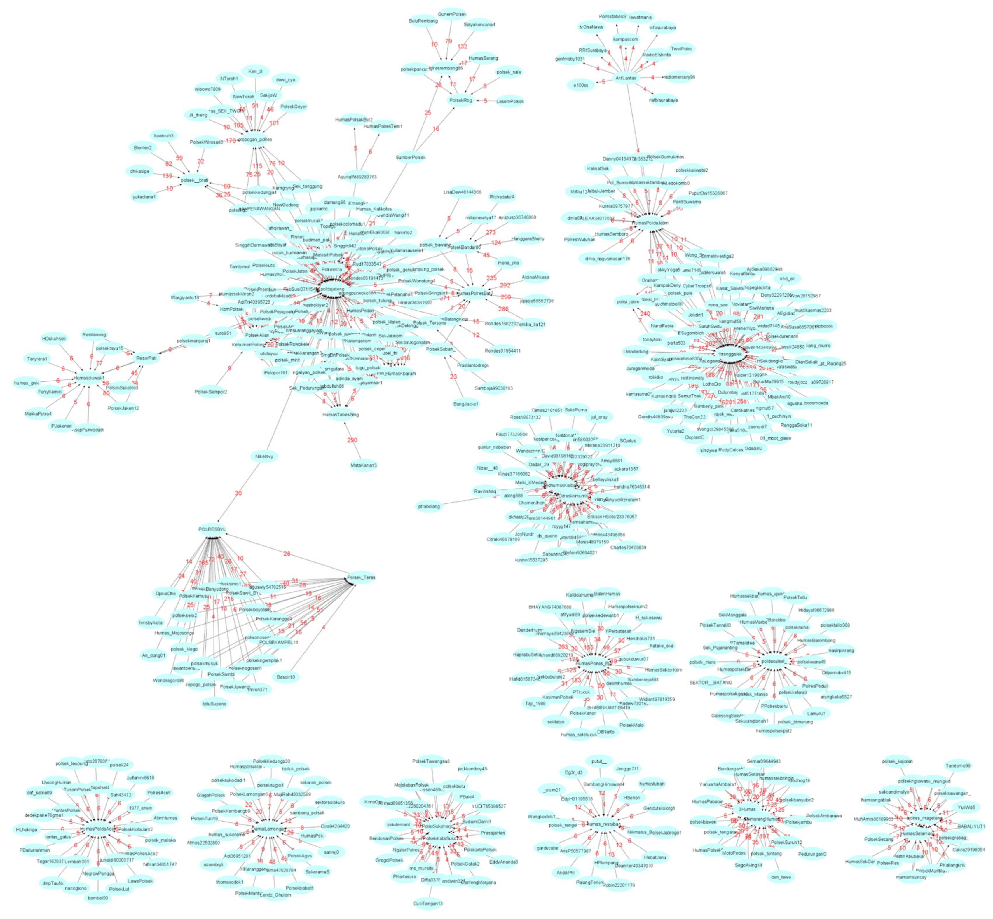
5.4. Finding and Discussion of SICs

We detected SIC using various in-degree threshold (thInDeg). As there were many SICs discovered, we present the sample SIC obtained using thInDeg = 5 and thInDeg = 10 (counts with users who are the center of communities) in

Table 4. Description of few SICs.

Graph	thInDeg	#SICs	Sample of SICs
			Center Id	#Members
gTweets-1	5	5	DamaiLamongan	21
			silentreadeer	7
			energitodayID	12
			CNNIndonesia	16
			RETHA_Monicaa	6
gTweets-2	5	1	restulungagung	6
gTweets-3	10	21	PolisiInfo	15
			humas_restuban	19
			Polres_Bwi	12
			Hpanunggalan	14
			HumasPolres_Bjn	24
gTweets-4	10	32	DitreskrimumK	33
			HumasPoldaAceh	30
			MatesihPolsek	11
			poldajateng	92
			poldasulsel_	30
gTweets-5	5	4	PolisiInfo	12
			HumasPolres_Bjn	16
			1trenggalek	10
			poldajateng	23

. The execution times of the first to fifth graphs are 1.51, 1.98, 1.86, 1.24, and 1.63 s. This shows that the GraphFrame parallel query employed in the algorithm is efficient.

As shown on Table 4, many SIC communities are found in the graphs of 28 February–6 March (gTweets-2) and 7–13 March 2021 (gTweets-4). This is in line with Table 3, where there are many nodes having a high in-degree and out-degree.

Discussion and Analysis of the SICs

The active communities may change from period to period. At the end of January 2021, the communities were news users (CNN), while in March 2021, there were many police officers from many provinces that formed the communities. Further observation of each member of the communities shows that each center of the “police SIC” received lots of reply or quote tweets from either civilians or other police offices. This shows the insight that in Indonesia, police officers are active Twitter users and gain lots of responses when they send tweets related to COVID-19. Based on these findings, further analyses can be performed (such as using NLP to mine the tweet texts for each period) in order to find linkages between the communities and the tweets’ content.

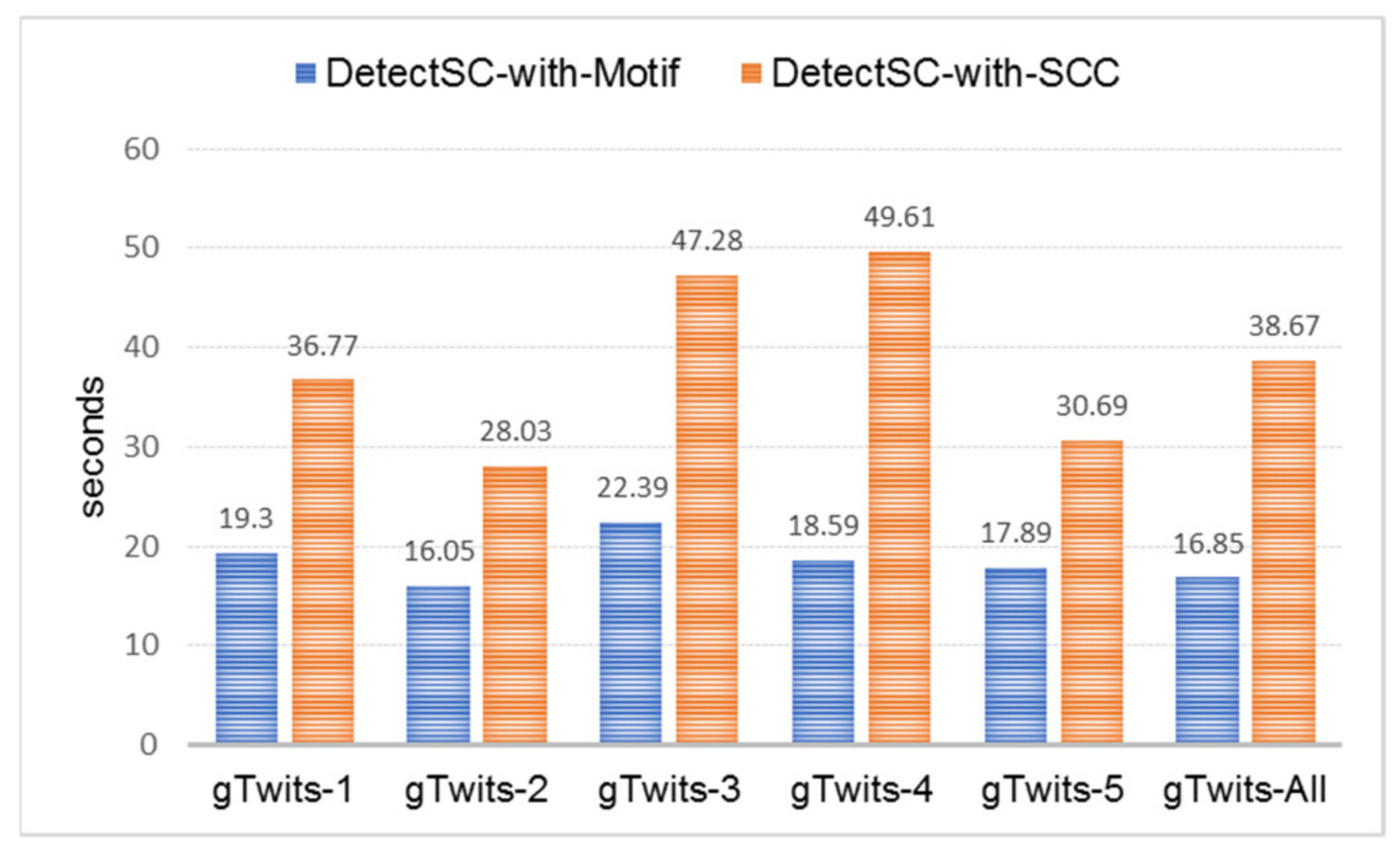
5.5. Finding and Discussion of SCs and SICs

There are many SCs and SCICs uncovered from the prepared graphs, as depicted on

Table 5. SC and SCIC discovered from 2 graphs.

Graphs/#Communities	SC: #Members: Id Members	SCIC: #Members: Id Members
gTweets-1/ 6	2: penyejuk_hati_ DariusSastro; 2: RETHA_Monicaa silentreadeer; 3: mhd_arisashari Ndrews1162011 dewis207; 2: HandriAs8 CrbSira, 3: AProletarian anakodok2009 hadifianwidjaja; 2: Korban_Rezim Tarida_Indah	2: penyejuk_hati_ DariusSastro, 8: orangdesadamai SwanLakee8 KIMLIE_8 RETHA_Monicaa keevan03 silentreadeer Chaterinee_08 perahukertas97; 4: mhd_arisashari arits_0301 Ndrews1162011 dewis207; 2: HandriAs8 CrbSira; 3: AProletarian anakodok2009 hadifianwidjaja; 4: Panglima_Minal Korban_Rezim Tarida_Indah Oposisi_Kecil
gTweets-2/ 3	2: akundihackmulu jtuvanyx; 2: sek_pemalang polres_pemalang; 2: Fido_Dildo emha_baraja	2: akundihackmulu jtuvanyx; 2: sek_pemalang polres_pemalang; 2: Fido_Dildo emha_baraja

and Appendix A,

Table A1. SC and SCIC Communities of 3 graphs.

Graphs/#Communities	SC: #Members: Id Members	SCIC: #Members: Id Members
gTweets-3/ 4	2: PolresKra MatesihPolsek; 2: dfitriani1 Trikus2012; 2: sek_pemalang polres_pemalang; 2: putu_ardikabali KakBejo	10: MatesihPolsek polsekcolomadu1 Hanafi0101 PolresKra poldajateng_ Rud17833547 Sek_Mojogedang Topage19 agungpurwoko186 cucuk_kurniawan; 3: dfitriani1 HannyValenciaa Trikus2012; 10: Jonatan77875470 Warungpring1 poldajateng_ tyas_aldian Wiekha5 sek_pemalang HumasWatukumpul polres_pemalang Anto60king sakila2021 3_Martha23 TiaraJelita20; 2: putu_ardikabali KakBejo
gTweets-4/ 4	2: 3Humas SemarangHumas; 2: Kfaizureen Mat_Erk; 3: HumasPoldaRiau BastianusRicar3 Hans77759603; 2: rokandt Alva47831808	20: 3Humas BandunganH PolsekAmbarawa PedurunganO TeloGodhog18 polsek_tengaran PolsekSuruh12 den_tewe SegoAking14 SemarangHumas HumasPolsekSum7 polsekbanyubir2 polsek_tuntang HPolsekjambu HumasGetasan polsekbawen YanuartaAmbara1 HumasPabelan humassekbringin Semar09644943 MotoPedes, 3: Kfaizureen ffiekahishak Mat_Erk; 3: HumasPoldaRiau BastianusRicar3 Hans77759603; 2: rokandt Alva47831808
gTweets-5/ 3	2: ___327____ syarlothsita; 2: tejomament BabylonGate1; 2: equalgame97 chibicatsaurus	4: ___327____ syarlothsita rokandt arifbsantoso; 2: tejomament BabylonGate1; 2: equalgame97 chibicatsaurus

. For detecting SCs, we ran Algorithm 2 using six patterns, shown in Figure 3 (Section 3). For detecting SCICs, we ran Algorithm 8 using 2 SC patterns found in SCs, which are Cyclic_2(“(a)-[e1]->(b); (b)-[e2]->(a)”) and Cyclic_22 (“(a)-[e1]->(b); (b)-[e2]->(c); (c)-[e3]->(b); (b)-[e4]->(a)”).

Our proposed techniques are based on dataframe query, SCC algorithm, and GraphFrames motif findings on Spark, which have been fully tested. To evaluate the SC and SIC results, we simply compared the communities’ and the graphs’ visualization as generated with Cystoscape (https://cytoscape.org/, accessed on 6 April 2021), as presented on Figure 8 and Figure A2. All of the computation results (Table 5 and Table A1) match with the graphs’ visualizations. For instance, six SCs and SCICs of gTweets-1 (with members shown on Table 5) comply with the graphs shown in Figure 8.

The execution times of those two algorithms in processing each graph are depicted in Figure 8 and Figure 9. Algorithm 2 (DetectSC-with-MotifFinding) ran faster compared to Algorithm 4 (DetectSC-with-SCC). Using motif findings, as more patterns were used to discover, execution was slower, because Spark performed more hash-join operations among dataframes. By comparing Figure 9 and Figure 10, it can be observed that on running Algorithm 4, most of the execution time was needed to find the strongly connected sub-graphs; the hash-join operations for finding vertices’ neighbors (Step 7–10) needed a lot less execution time.

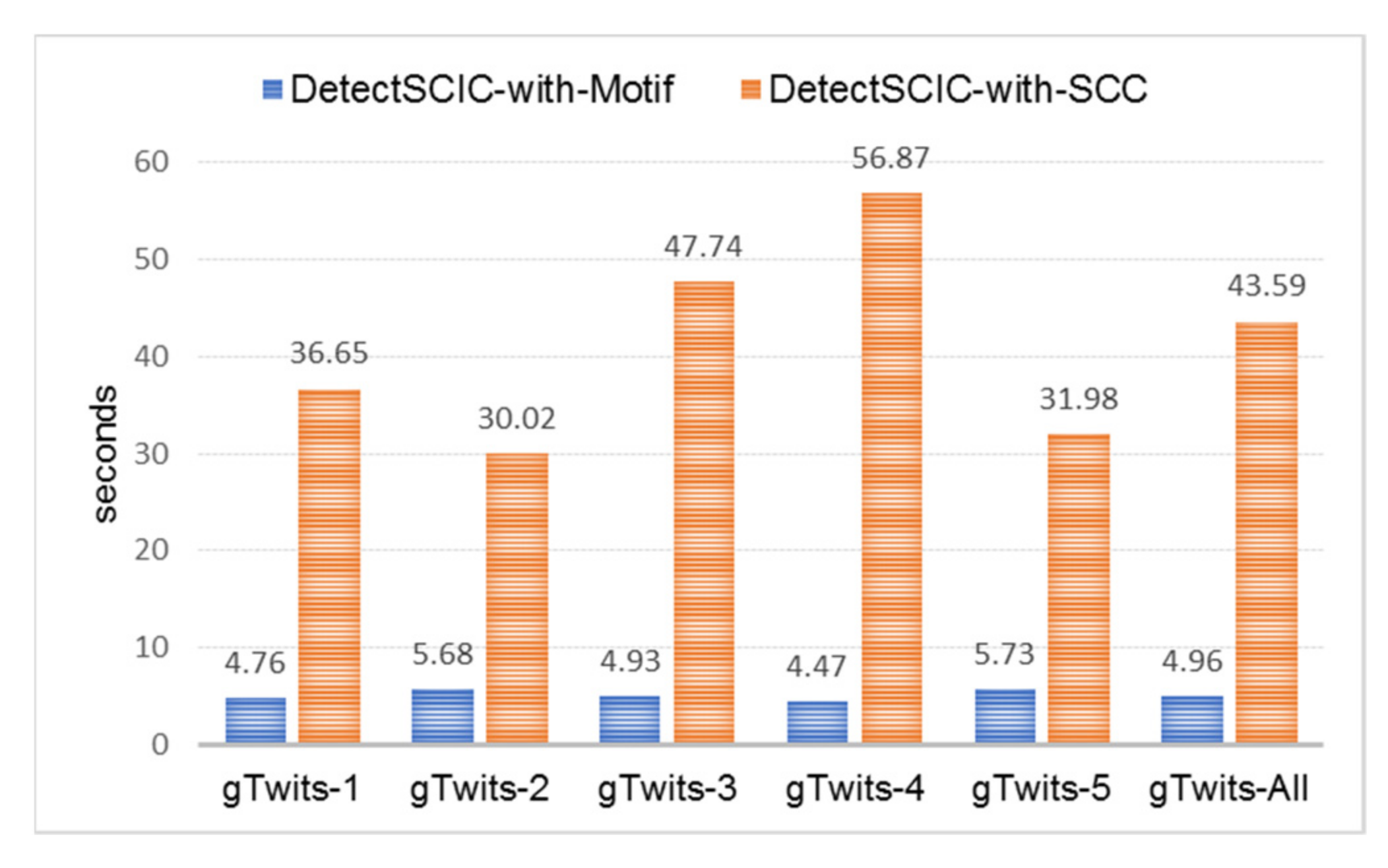
5.5.1. Discussion and Analysis of the SCs and SCICs

Compared to the SICs found (Table 4), the number of SCs and SCICs found were far smaller; there were only a few members in each community. However, since these communities conducted intense communication (via replying and quoting tweets), each community had a stronger relationship. By checking the corresponding username and attributes, we uncovered that the SC formed for each period could be characterized as follows:

(1)

24–30 January and 14–20 March 202: civilian-only communities were formed.

(2)

21–27 February 2021: civilian-only and police officer-only communities were formed.

(3)

28 February–6 March and 7–13 March 2021: civilian-only and civilian-police officer communities were formed.

Thus, in Indonesia, there were times when police officers interacted (via reply and quote) with each other frequently, forming temporal active communities.

On the other hand, each of the SCICs formed (that include SCs and their neighbors, if any) had either civilian members only or police officers and civilians together. This means that tweets from police officers on particular topics also attracted civilians, so that they drew intensive responses.

Following discovery of SCs and SCICs, further analysis can be conducted using other techniques (i.e., Natural Language Processing) to find the tweets’ discussion topic or content which draw intense responses in the community.

These findings give insights into the response to the COVID-19 pandemic, as suggested in [29]. The Indonesian Special task force includes military and police forces; these findings regarding communities from tweets prove that the police have been successful in attracting lots of users to respond to their information, which is sent via tweet.

There are potential uses for these findings. As discussed in [30], Taiwan is an example of a country that responded quickly to the pandemic crisis. Through early recognition of the crisis, daily briefings to the public, and simple health messaging, the government was able to reassure the public by delivering timely, accurate, and transparent information regarding the evolving epidemic. Having found those active communities with their “core members”, in this case, the core members can be employed or targeted to help distribute the information more effectively.

5.5.2. The Scalability Issue

As the overall time complexities of our proposed algorithms cannot be derived yet due to the lack of SCC algorithm complexity, the execution times (Figure 9 and Figure 10) have not been analyzed using their complexities. The scalability of the proposed algorithms has not been discussed based on time complexities. Rather, our view of this issue is as follows: it is known that large networks follow power law distributions (there are few nodes with high interactions and the rest are nodes with less or low interactions). In our proposed algorithms, this property is adopted in the data preparation step (Step-1), which produces smaller sizes of graphs. Using dataframes and Spark SQL, the parallel filtering in the data preparation is performed with approximately O(n/p). The complex computations are performed in the next steps that call motif finding or SCC algorithms. By feeding smaller graphs than the original raw graphs to the parallel motif finding and SCC algorithms, we expect that these graphs can be handled to detect communities.

6. Conclusions and Further Works

In Spark, simple queries can be used to find SICs from weighted directed graphs, and its computation is fast. GraphFrames motif finding and a strongly connected component algorithm can be employed to discover active communities, SCs and SCICs, from the graphs. Pros and cons include: (1) the motif finding approach has limitations in that the subgraph patterns (representing the core community members) should be defined in advance, but its computation is fast if only a few patterns are used to find strongly connected subgraphs; (2) the parallel strongly connected component algorithm is complex, requires more machine and network resources, and is slower, but it is able to find strongly connected subgraphs with previously unknown connection patterns. Thus, when fast graph processing is needed, the algorithm can be run towards sample graphs; after the subgraph patterns are found, these can be used to process the whole graphs, or the next graphs if the dataset is processed periodically.

From the case study, we have demonstrated that directed weighted graphs can be prepared from streams of tweets, which can then be mined to find useful temporal active communities. Similar approaches can be applied to other cases, where data representing peoples’ interactions from time to time (such as via comments, messaging and so forth) are recorded.

The unresolved issue in this research is deriving time complexity for each of the proposed algorithms. Further work is needed to analyze the algorithms’ scalability using their complexities. With its speedy computation in finding connected components, GraphFrames motif finding possesses the potency to be used for uncovering active temporal communities from batches of data stream coming in with high velocity, when results are needed in near-real time. It is possible to avoid delay that can accumulate between a batch and the next batch in processing, which is an important issue in processing big data streams. In such a system, Structured Streaming, which is a stream processing framework built on the Spark SQL engine [6], can be used together with GraphFrames motif finding.

References

1. Bae, S.-H.; Halperin, D.; West, J.D.; Rosvall, M.; Howe, B. Scalable and Efficient Flow-Based Community Detection for Large-Scale Graph Analysis. ACM Trans. Knowl. Discov. Data 2017, 11, 1–30. [Google Scholar] [CrossRef]
2. Fortunato, S. Community detection in graphs. In Complex Networks and Systems Lagrange Laboratory; ISI Foundation: Torino, Italy, 2010. [Google Scholar]
3. Makris, C.; Pispirigos, G. Stacked Community Prediction: A Distributed Stacking-Based Community Extraction Methodology for Large Scale Social Networks. Big Data Cogn. Comput. 2021, 5, 14. [Google Scholar] [CrossRef]
4. Yao, K.; Papadias, D.; Bakiras, S. Density-based Community Detection in Geo-Social Networks. In Proceedings of the 16th International Symposium on Spatial and Temporal Databases (SSTD’19), Vienna, Austria, 19–21 August 2019. [Google Scholar]
5. Malak, M.S.; East, R. Spark GraphX in Action; Manning Publ. Co.: Shelter Island, NY, USA, 2016. [Google Scholar]
6. Chambers, B.; Zaharia, M. Spark: The Definitive Guide, Big Data Processing Made Simple; O’Reilly Media, Inc.: Sebastopol, CA, USA, 2018. [Google Scholar]
7. Atastina, I.; Sitohang, B.; Saptawati, G.A.P.; Moertini, V.S. An Implementation of Graph Mining to Find the Group Evolution in Communication Data Record. In Proceedings of the DSIT2018, Singapore, 20–22 July 2018. [Google Scholar] [CrossRef]
8. Dave, A.; Jindal, A.; Li, L.E.; Xin, R.; Gonzalez, J.; Zaharia, M. GraphFrames: An Integrated API for Mixing Graph and Relational Queries. In Proceedings of the Fourth International Workshop on Graph Data Management Experiences and Systems, Redwood Shores, CA, USA, 24 June 2016. [Google Scholar] [CrossRef]
9. Tran, D.H.; Gaber, M.M.; Sattler, K.U. Change Detection in Streaming Data in the Era of Big Data: Models and Issues. SIGKDD Explorations. 2014. Available online: https://www.kdd.org/explorations/view/june-2014-volume-16-issue-1 (accessed on 27 February 2021).
10. Moertini, V.S.; Adithia, M.T. Pengantar Data Science dan Aplikasinya bagi Pemula; Unpar Press: Bandung, Indonesia, 2020. [Google Scholar]
11. Fung, P.K. InfoFlow: A Distributed Algorithm to Detect Communities According to the Map Equation. Big Data Cogn. Comput. 2019, 3, 42. [Google Scholar] [CrossRef] [Green Version]
12. Bhatt, S.; Padhee, S.; Sheth, A.; Chen, K.; Shalin, V.; Doran, D.; Minnery, B. Knowledge Graph Enhanced Community Detection and Characterization. In Proceedings of the 12th ACM International Conference on Web Search and Data Mining (WSDM ’19), Melbourne, VIC, Australia, 11–15 February 2019. [Google Scholar] [CrossRef]
13. Jia, Y.; Zhang, Q.; Zhang, W.; Wang, X. CommunityGAN: Community Detection with Generative Adversarial Nets. In Proceedings of the International World Wide Web Conference (WWW ’19), San Francisco, CA, USA, 13–17 May 2019. [Google Scholar]
14. Roghani, H.; Bouyer, A.; Nourani, E. PLDLS: A novel parallel label diffusion and label selection-based community detection algorithm based on Spark in social networks. Expert Syst. Appl. 2021, 183, 115377. [Google Scholar] [CrossRef]
15. Zhang, Y.; Yin, D.; Wu, B.; Long, F.; Cui, Y.; Bian, X. PLinkSHRINK: A parallel overlapping community detection algorithm with Link-Graph for large networks. Soc. Netw. Anal. Min. 2019, 9, 66. [Google Scholar] [CrossRef]
16. Corizzo, R.; Pio, G.; Ceci, M.; Malerba, D. DENCAST: Distributed density-based clustering for multi-target regression. J. Big Data 2019, 6, 43. [Google Scholar] [CrossRef]
17. Krishna, R.J.; Sharma, D.P. Review of Parallel and Distributed Community Detection Algorithms. In Proceedings of the the 2nd International Conference on Information Management and Machine Intelligence (ICIMMI), Jaipur, Rajasthan, India, 24–25 July 2020. [Google Scholar] [CrossRef]
18. Sadri, A.M.; Hasan, S.; Ukkusuri, S.V.; Lopez, J.E.S. Analyzing Social Interaction Networks from Twitter for Planned Special Events; Lyles School of Civil Engineering, Purdue University: West Lafayette, IN, USA, 2017. [Google Scholar]
19. Karau, H.; Warren, R. High Performance Spark; O’Reilly Media, Inc.: Sebastopol, CA, USA, 2017. [Google Scholar]
20. Holmes, A. Hadoop in Practice; Manning Publications, Co.: Shelter Island, NY, USA, 2012. [Google Scholar]
21. White, T. Hadoop: The Definitive Guide, 4th ed.; O’Reilly Media, Inc.: Sebastopol, CA, USA, 2015. [Google Scholar]
22. Karau, H.; Konwinski, A.; Wendell, P.; Zaharia, M. Learning Spark; O’Reilly Media, Inc.: Sebastopol, CA, USA, 2015. [Google Scholar]
23. Moertini, V.S.; Ariel, M. Scalable Parallel Big Data Summarization Technique Based on Hierarchical Clustering Algorithm. J. Theor. Appl. Inf. Technol. 2020, 98, 3559–3581. [Google Scholar]
24. Gonzalez, J.E.; Xin, R.S.; Dave, A.; Crankshaw, D. GraphX: Graph Processing in a Distributed Dataflow Framework. In Proceedings of the 11th USENIX Symposium on Operating Systems Design and Implementation (OSDI’14), USENIX Association, Denver (Broomfield), CO, USA, 6–8 October 2014; pp. 599–613. [Google Scholar]
25. Yan, D.; Cheng, J.; Xing, K.; Lu, Y.; Ng, W.S.H.; Bu, Y. Pregel Algorithms for Graph Connectivity Problems with Performance Guarantees. In Proceedings of the 40th International Conference on Very Large Data Bases, Hangzhou, China, 1–5 September 2014. [Google Scholar]
26. Bahrami, R.A.; Gulati, J.; Abulaish, M. Efficient Processing of SPARQL Queries Over GraphFrames. In Proceedings of the IEEE/WIC/ACM International Conference on Web Intelligence (WI’17), Leipzig, Germany, 23–26 August 2017; pp. 678–685. [Google Scholar]
27. Balkesen, C.; Teubner, J.; Alonso, G.; Ozsu, M.T. Main-Memory Hash Joins on Modern Processor Architectures. IEEE Trans. Knowl. Data Eng. 2015, 27, 1754–1766. [Google Scholar] [CrossRef] [Green Version]
28. McAuley, J.; Leskovec, J. Learning to Discover Social Circles in Ego Networks; Stanford University: Stanford, CA, USA, 2012. [Google Scholar]
29. Djalante, R.; Lassa, J.; Setiamarga, D.; Sudjatma, A.; Indrawan, M.; Haryanto, B.; Mahfud, C.; Sinapoy, M.S.; Djalante, S.; Rafliana, I.; et al. Review and analysis of current responses to COVID-19 in Indonesia: Period of January to March 2020. Prog. Disaster Sci. 2020, 6, 100091. [Google Scholar] [CrossRef] [PubMed]
30. Wang, C.J.; Ng, C.; Brook, R.H. Response to COVID-19 in Taiwan, Big Data Analytics, New Technology, and Proactive Testing. JAMA 2020, 323, 1341. [Google Scholar] [CrossRef] [PubMed]
Figure 1. The Spark application tree [23].
Bdcc 05 00046 g001
Figure 2. Illustration of shuffling for a stage on a Spark cluster with four workers: each worker stores one RDD partition and runs a map task, then two reducer tasks on two workers process data from map tasks.
Bdcc 05 00046 g002
Figure 3. Six SCC subgraphs to be detected from graph dataset: (a) g1, (b) g2, (c) g3, (d) g4, (e) g5, (f) g6.
Bdcc 05 00046 g003
Figure 4. The DAG of motif finding of SCC from g1, Cyclic_2.
Bdcc 05 00046 g004
Figure 5. Execution time of motif finding vs. SCC algorithm.
Bdcc 05 00046 g005
Figure 6. Illustration of active communities formed from a weighted-directed graph with threshold of edge weight = 4.
Bdcc 05 00046 g006
Figure 7. The architecture of data collection system.
Bdcc 05 00046 g007
Figure 8. Some part of the clean and filtered-weighted-directed graph, gTweets-1.
Bdcc 05 00046 g008
Figure 9. Execution time of detecting SCs.
Bdcc 05 00046 g009
Figure 10. Execution time of detecting SCICs.
Bdcc 05 00046 g010