Article

PerTract: Model Extraction and Specification of Big Data Systems for Performance Prediction by the Example of Apache Spark and Hadoop

1
fortiss, Research Institute of the Free State of Bavaria, Guerickestr. 25, 80805 Munich, Germany
2
Chair for Information Systems, Technical University of Munich (TUM), Boltzmannstr. 3, 85748 Garching, Germany
*
Author to whom correspondence should be addressed.
Big Data Cogn. Comput. 2019, 3(3), 47; https://doi.org/10.3390/bdcc3030047
Submission received: 13 July 2019 / Revised: 2 August 2019 / Accepted: 6 August 2019 / Published: 9 August 2019

Abstract

:
Evaluating and predicting the performance of big data applications are required to efficiently size capacities and manage operations. Gaining profound insights into the system architecture, dependencies of components, resource demands, and configurations cause difficulties to engineers. To address these challenges, this paper presents an approach to automatically extract and transform system specifications to predict the performance of applications. It consists of three components. First, a system-and tool-agnostic domain-specific language (DSL) allows the modeling of performance-relevant factors of big data applications, computing resources, and data workload. Second, DSL instances are automatically extracted from monitored measurements of Apache Spark and Apache Hadoop (i.e., YARN and HDFS) systems. Third, these instances are transformed to model- and simulation-based performance evaluation tools to allow predictions. By adapting DSL instances, our approach enables engineers to predict the performance of applications for different scenarios such as changing data input and resources. We evaluate our approach by predicting the performance of linear regression and random forest applications of the HiBench benchmark suite. Simulation results of adjusted DSL instances compared to measurement results show accurate predictions errors below 15% based upon averages for response times and resource utilization.

1. Introduction

Big data frameworks are specialized to analyze data with high volume, variety, and velocity efficiently [1]. By distributing and parallelizing processing, they allow for horizontal scalability. Since the introduction of the MapReduce paradigm, there have been several frameworks released to support different types of applications, such as machine learning and stream processing. For all types, the performance of such software systems in terms of response time, throughput, and resource utilization is essential for a successful application [2]. It is a difficult and complex task to manage and evaluate the performance for different scenarios such as changing data input and hardware resources [3].
Practical evaluations such as load tests on test systems are expensive. They require multiple experiments and only test a subset of configuration parameters. Additionally, they usually run with a reduced amount of data and resources. Thus, it is not able to draw accurate conclusions about the performance behavior. Performance models, on the other hand, provide an established evaluation approach by depicting performance characteristics of software systems and simulating their behavior or analytically solving them [4]. However, there are several challenges: creating models by hand is expensive, error-prone and slow as software systems are complex and continuously evolve [5]. There is a lack of tool support for automatic model extraction. Regarding big data system, most related modeling approaches are also specific to a certain technology (i.e., Apache MapReduce) and only consider the response time of applications but not demands for resources (i.e., CPU).
In order to address these challenges, we propose a specification and model extraction approach for big data systems called PerTract to evaluate and predict the performance. We present a domain-specific language (DSL) to allow for modeling specifications on an architecture-level in a tool-agnostic way. To demonstrate our approach, we use Apache Spark for the application layer, in particular one random forest and one linear regression application that both use Spark’s machine learning library. Additionally, we use Apache Hadoop for data provisioning and resource management. Figure 1 illustrates an overview of our approach. We extract execution components and inter-component interactions, resource landscape, and data workload in three separated specifications of a DSL instance using interfaces and logs of these technologies. In addition, we extract monitoring traces of applications (i.e., CPU times) and interrelate these with data workload information to identify parametric dependencies and estimate parametric resource demands of each execution component. On this basis, performance predictions are enabled. Therefore, we transform a DSL instance into a Palladio component model (PCM) [6]. Palladio is a model-based performance evaluation tool on the architecture-level that is supported by several analytical solvers and simulation engines.
Our approach provides several benefits. It integrates model-based activities, which are performed during development, and measurement-based activities, which are carried out during operations (DevOps) [5]. The automated extraction process eliminates the effort to create models by hand. As applications are continuously updated, DSL instances can be extracted and tracked for each release as they evolve as well. This also enables engineers to continuously manage and plan required capacities and evaluate the performance for different scenarios (e.g., changing data workload) by adapting model parameters. Finally, it gives detailed insights about resource demands of execution components of an application and can be used to detect performance changes and regressions.
To sum up, the contributions of this paper are the following:
  • A DSL for modeling performance-relevant factors of big data systems,
  • An automatic extraction of system structure, behavior, resource demands, and data workload from Apache Spark and Apache Hadoop,
  • Transformations from DSL instances to model- and simulation-based performance evaluation tools,
  • Tool support for this approach.
To the best of our knowledge, our approach is the first white-box approach to extract performance-relevant metrics that allow for performance predictions of response times and resource usage. The developed tools are open source [7] and extendable for extracting DSL instances from other frameworks and for transforming them to other model-based performance evaluation tools.
This paper builds upon our previous work [8,9,10,11] on modeling and simulating the performance of big data applications and includes the following major improvements and extensions:
  • A formalism and DSL to model big data applications,
  • A lightweight Java agent to sample stack traces and CPU times from applications,
  • Automatic extraction of DSL instances,
  • Detailed evaluation against complex applications of the HiBench benchmark suite.
The remainder of this work is structured as follows: Section 2 describes related literature and approaches in the area of modeling and simulating big data applications. Section 3 introduces the model formalism as well as the DSL, which are required to understand this paper. Section 4 describes the extraction of DSL instances by the example of Apache Spark and Apache Hadoop. Section 5 presents the transformation to PCM models to allow for simulating the performance. Section 6 evaluates the prediction accuracy of our proposed approach for different upscaling scenarios and describes our assumptions and limitations. Finally, Section 7 outlines conclusions of our work and ideas for future activities.

2. Related Work

Since the Apache Hadoop family was the first widely-adopted big data framework, initial performance modeling approaches have been concentrating on this technology stack.
Vianna et al. [12] predict the response time of MapReduce applications by introducing an analytical model, which they validated against an event-driven queuing network simulator. Their approach primarily concentrated on synchronization delays between map and reduce tasks. Verma et al. [13] introduce another approach for MapReduce. They developed a framework to allow for predicting response times before moving applications to different target platforms. The framework applies multiple benchmarks on source platforms and a regression-based model to relate the performance of source and the target platforms. Zhang et al. [14,15,16] present multiple approaches where most of them are based on the analytical model by [13]. Therefore, they additionally take heterogeneous clusters and configuration optimizations into account.
For other applications of the Hadoop family, Barbierato et al. [17] developed a language for the description of performance models. As a main component, the model uses the SQL-like query language of Apache Hive, a data warehouse built on top of Apache Hadoop. Ardagna et al. [18] propose approaches to estimate response times of Hive requirements. Therefore, they presented multiple performance analysis models with increasing complexity and accuracy, such as queueing networks and stochastic well formed nets. They also considered unreliable resources in their experiments. Lehrig [19] proposes a scalability and elasticity analysis of Software-as-a-Service applications at design time using architectural templates for Palladio. They plan to enhance it for big data paradigms on the processing layer and data layer.
Wang and Khan [3] propose a prediction model for estimating response times of Apache Spark applications. In their approach, they consider demands for in-memory as well as demands for disk drives but not CPU processing. Another work by Ardagna et al. [20] explores three modeling approaches for execution time prediction of Spark applications: one queuing network with a fork-join model and one with a task precedence model. Third, they present a discrete event simulation engine dagSim. The evaluation was conducted for different applications such as logistic regression and K-Means running in a public cloud. Although the variance of the prediction accuracy is low for all approaches, the third approach delivers the most precise results.
Besides analytical and simulation-driven approaches, there are also approaches using machine learning for Apache Spark. Rekha and Praveen [21] evaluated different machine learning algorithms (i.e., multi linear regression and support vector machine) as well as an analytical model to predict execution times of Spark stages in development environments. They include multiple parameters from application logs into their models but only use execution times and do not consider resource demands. They also mention the drawback of machine learning approaches, which require intensive experiments and data collection. Furthermore, Venkataraman et al. [22] present Ernest, a performance prediction framework for large scale analytics using machine learning kernels. It involves an automatic process to collect training data and to build a non-negative least squared model taking only a few parameters. They evaluate their approach on Amazon EC2 and show accurate predictions of execution times for increasing machine numbers. It is a black-box approach and does not give any insight into components of an application. As Ernest is bound to the structure of machine learning jobs, Alipourfard et al. [23] present CherryPick, which intends to find best cloud configurations for various applications and use Bayesian optimization to create performance models. A configuration, for instance, contains parameters such as the number of virtual machines, CPU, and cores. In contrast to our work, they support additional types of applications (i.e., Spark SQL). Additionally, Witt et al. [24] provide an extensive survey on performance prediction of batch processing using black box monitoring and machine learning.
Castiglione et al. [25] propose a general approach to model the behavior of batch applications and concentrate on cloud infrastructures and evolution dynamics in terms of resource requirements and energy consumption. Therefore, they use an analytic modeling technique based Markovian agents and mean field analysis to describe the behavior of interactive cloud, batch, and time constrained applications. Niemann [26] also presents an approach in the area of energy consumption. He focuses on Apache Cassandra, a distributed data management system, and uses queueing Petri nets to predict the performance and energy consumption of different workloads and platforms. Casale et al. [27] propose a model-driven engineering for quality assurance of data-intensive software systems concentrating on Apache Hadoop and MapReduce, NoSQL databases, and stream processing (i.e., Apache Storm). Their approach aims at simulating, verifying, and optimizing architectures of big data applications. The models contain three different model layers including a platform-independent, a technology-specific and a deployment-specific model [28]. Gómez et al. [29] also shows an approach to transform these models into stochastic Petri nets, which is intended to allow for evaluating performance requirements. Lastly, Ginis and Strom [30] hold a patent in the area of stream processing. The patent describes a method to model performance characteristics of publish–subscribe systems using queueing theory. However, the method does not include resource demands such as CPU, memory, and disks.
To summarize, the mentioned approaches focus on predicting the metric response time and often only implicitly assume resource demands for service executions per resource but do not link them to software components and operations [5]. To the best of our knowledge, automatic model extraction in the area of big data are only supported by the mentioned machine learning approaches [22,23]. However, these are black-box approaches and the models serve as interpolation of the measurements [5]. Consequently, they do not model detailed information of the system architecture and dependencies and cannot be adapted for further evaluation scenarios. Finally, most of the mentioned models are technology-specific and, thus, are difficult to adapt and generalize them.

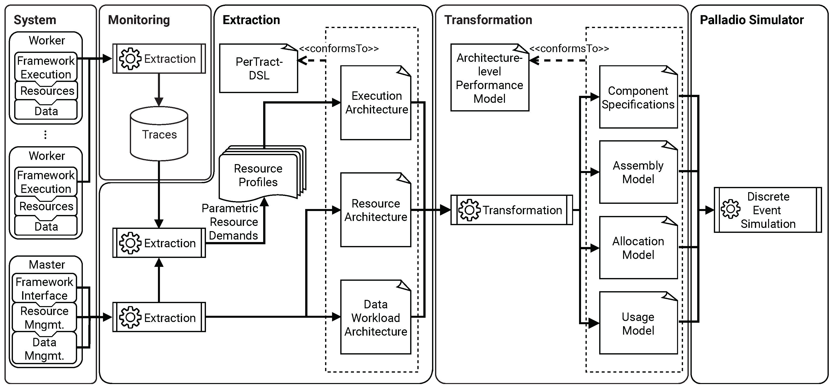
3. Modeling Approach
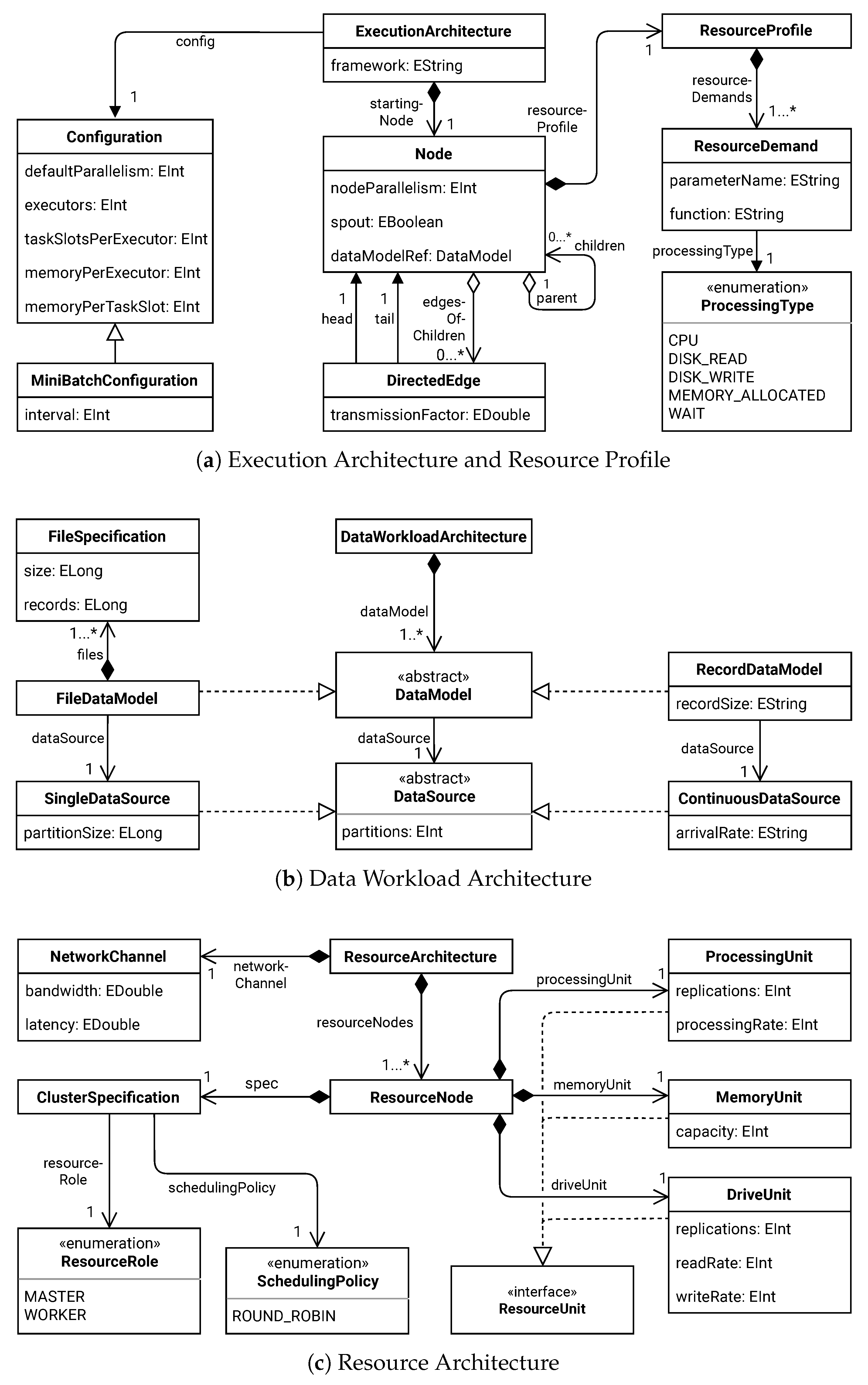
In this section, we describe the formalism for specifying big data systems. Afterwards, we present the PerTract-DSL based on the formalism.

3.1. Formalism

The specification consists of the following components:
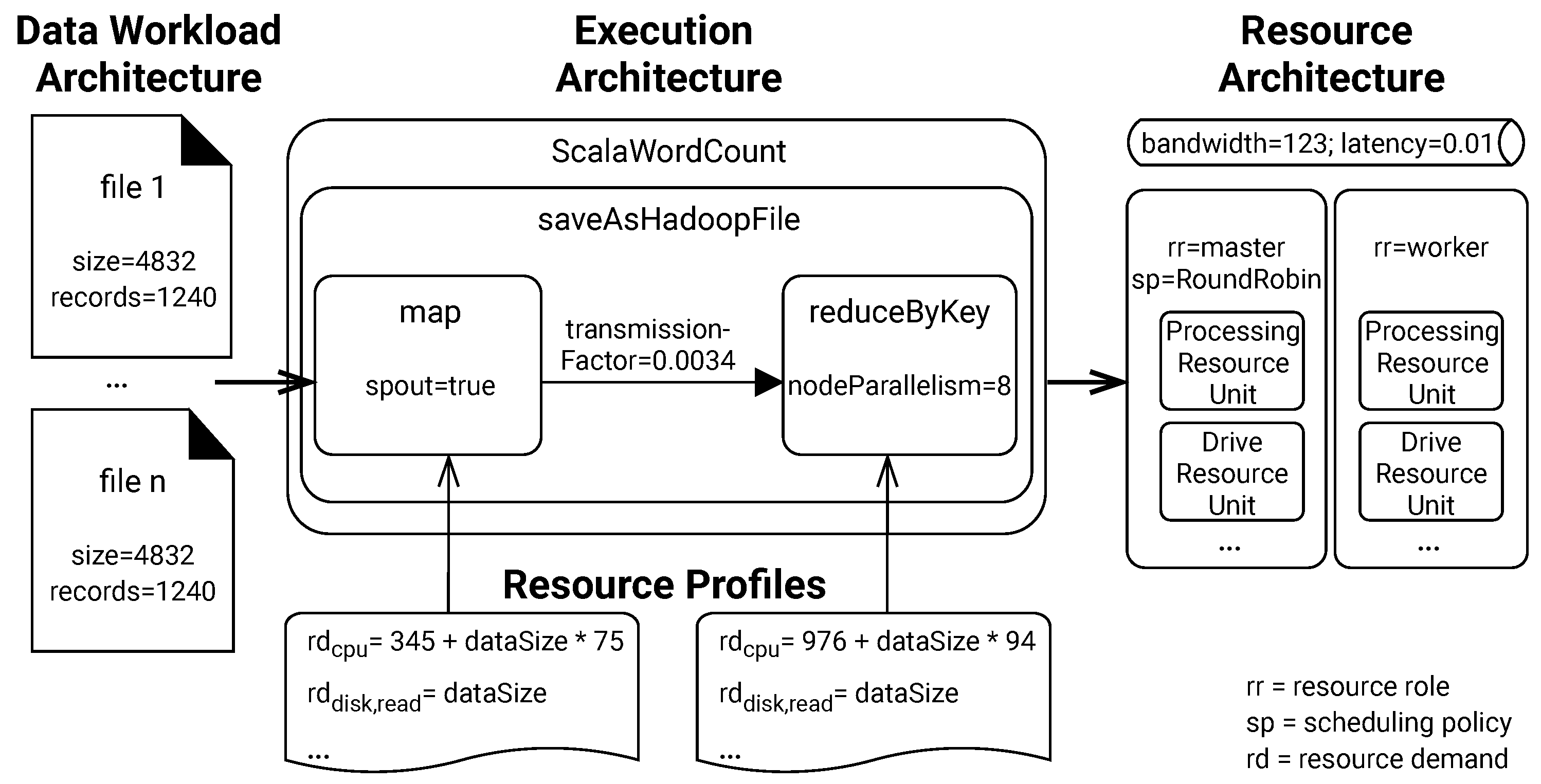
  • An Execution Architecture of the application, specifying nested directed graphs for execution components,
  • A set of Resource Profiles, providing demands of different resources with parametric dependencies for the nodes of a graph,
  • A Data Workload Architecture, specifying the underlying data model and type of data source
  • A Resource Architecture, specifying a cluster of resource nodes, each with several resource units

3.1.1. Application Execution Architecture

The specification of the application Execution Architecture is a 2-tuple ( c , n ) where c C is the application configuration and n N specifies an initial node of the application.
A configuration c C is represented by the 5-tuple ( p d , e , t s e , m e , m t s ) where p d is the default parallelism for operations, more specifically tasks, of an application (e.g., join or reduce); e is the number of executors, which manage tasks; t s e describes the number of tasks slots per executor that can be executed in parallel; m e is the amount of main memory per executor that is available for tasks; and m t s represents the amount of memory that each task slot requires to be allocated.
Nodes N are composite components. They can represent directed graphs N G N and execution nodes of a directed graph N E N . In Figure 2, ScalaWordCount and saveAsHadoopFile represent a directed graph and map and reduce an execution node.
A directed graph n g N G is a 2-tuple ( N n g , E n g ) , in which N n g is a set of nodes (or vertices) of the directed graph n g such that n g N n g ; and E n g is a set of directed edges. A directed edge e E is represented by a 3-tuple ( n t , n h , t e ) , where n t N is the tail of e; n h N is the head of e; and t e R 0 specifies the factor of how many data are transmitted from n t to n h dependent on the amount of input data of n t .
An execution node n e N E is a 5-tuple ( p n , s , m , n n g , r p ) where p n is the parallelism of node (e.g., some big data frameworks such as Apache Flink allow for specifying the parallelism for each operation individually); s indicates whether n e is a spout that is the node depending on partitioned data from an external source, such as a file system or messaging system; m M is a reference to the dependent data model from the Data Workload Architecture; n n g N G references the parent directed node graph; and r p R P describes the Resource Profile of n e .

3.1.2. Resource Profile

We use Resource Profiles to specify multiple resource demands. A Resource Profile r p R P describes an ordered set of parametric resource demands R D . A parametric resource demand r d R D is a 3-tuple ( r t , f r t , p ) in which r t R T represents the resource type and f r t : R 0 R 0 is a function to specify the actual value of a resource demand in dependence on a parameter p (e.g., number of partitions of an input data source).

3.1.3. Data Workload Architecture

The model to represent the data workload is kept very simple. A Data Workload Architecture d D is a singleton containing a set of data models M. A data model m M contains one data source d s D S element that consists of a parameter p d s to specify the number of partitions.

3.1.4. Resource Architecture

A Resource Architecture r a R A is a pair ( n c , R N ) in which n c N C is a network channel and R N is a set of resource nodes. A network channel n c N C is a 2-tuple ( b , l ) where b describes its bandwidth and l its latency. A resource node r n R N describes a cluster node and is a 2-tuple ( c s , R U ) in which c s C S is a cluster specification and R U is a set of resource units. A cluster specification c s C S is described by a 2-tuple ( r r , s p ) where r r R R describes a resource role (i.e., master node or worker node) and s p S P the scheduling policy for distributing task across resource nodes (i.e., round robin). A resource unit r u R U represents CPU, drive, and memory units.

3.2. PerTract-DSL

The PerTract-DSL follows the system model formalism described in the previous subsection and constitutes a language for specifying such models. Figure 2 illustrates an exemplary PerTract-DSL instance for a big data application. The PerTract-DSL is implemented as an Ecore-based meta-model using the Eclipse Modeling Framework (EMF) [31]. We use the DSL as an intermediate language to extract model instances and adapt its parameters for different scenarios. Afterwards, we generate architecture-level performance models that we use to simulate and predict the performance.
Figure 3a shows the classes and relationships of the Execution Architecture and Resource Profile. The Execution Architecture includes execution flows and operations on data and a configuration of an application. The configuration includes multiple parameters to specify the application settings. Depending on the application type (i.e., batch, mini-batch, and stream), a corresponding configuration type can be instantiated and may include additional parameters. For instance, a MiniBatchConfiguration involves an interval variable to indicate the mini-batch intervals.
In order to specify operations on data and execution flows, we use nodes and directed edges (for instance, distributed acyclic graphs DAGs represent execution flows in Apache Spark, topologies in Apache Storm, and job graphs and execution graphs in Apache Flink). Therefore, a Node is a composite that can represent two roles—a directed graph that contains several nodes (children) and edges, and an execution node that executes tasks. In the latter case, a node contains a Resource Profile for its tasks.
The term Resource Profile describes a set of resource demands for transactions of an application [32,33,34]. This includes resource demands for CPU, disk, memory, and network usage. Resource Profiles have been used for transactions for a specific workload and specific servers [32,33] but also for component operations within the control flow of each transaction independent of their deployment topology [34]. Branches with probabilities for its occurrences represent operation control flows. As yet, the related approaches do not use parametric dependencies and use Resource Profiles in the area of enterprise applications, where the workload is mainly user-driven and the resource demands for operations may remain static for each user. In our case, operations highly depend on incoming data volume either dependent on the data size or number of records.
We change the notion of Resource Profiles for our purposes in three ways. First, we include parametric dependencies. Second, we do not model the control flow and probability as this information is contained in the directed graph. Third, we do not apply a Resource Profile on the same fine granularity level of operations except for a set of operations and tasks. Big data frameworks chain and group single operations together and transform each grouping into a set of tasks, which will eventually be executed multiple times in a distributed way. The number of executed tasks usually depends on the number of partitions. As we model data and hardware resources as first-class entities in dedicated specifications, the exact number and distribution of operations depends on them. Therefore, we apply a Resource Profile on a group of chained operations. It forms the basis to derive tasks with resource demands and predict the performance by combining them with data workload and Resource Architectures.
While considering data as first-class entities, we focus on specifying only performance-relevant factors of data as presented in Figure 3b. A Data Workload Architecture contains one or several data models, which are either file-based (e.g., for batch applications) or record-based (e.g., for stream applications). The former contains multiple file specifications and a single data source, which specifies the partition size of the files and the number of partitions. The latter contains a variable to indicate the mean record size and a continuous data source, which describes the number of partitions of a data stream as well as the arrival rate per second of one record.
Figure 3c illustrates an overview of the classes and relationships of the Resource Architecture. It is a simplified version based on the resource environment model of PCM including our extension [6,9]. It contains several resource nodes that, combined, represent a cluster. Each resource node contains a processing unit, memory unit, and drive unit with individual processing rates or capacities. The resource demands of one Resource Profile will be performed on the corresponding resource units of one resource node.

4. Extracting Model Instances by the Example of Apache Spark, Apache YARN and Apache HDFS

Since creating models for applications, data, and resources requires much effort, we propose an approach to automatically extract PerTract-DSL instances based on monitoring measurements and logs. The remainder of this section describes the approach to extract a DSL instance in detail, comprising the monitoring on application level (Section 4.1), the extraction of Execution Architectures from applications (Section 4.2), the estimation of Resource Profiles for stages of applications (Section 4.3), the derivation of Data Workload Architectures (Section 4.4), and the extraction of hardware resources (Section 4.5).

4.1. Extraction of Resource Demands

Collecting measurement data is necessary in order to extract Resource Profiles, estimate resource demands, and calculate parametric dependencies. Profilers provide a common way to extract fine-grained data such as stack traces and CPU times. We examined multiple Java profilers but found that the performance of big data applications is significantly increased by their overhead. Therefore, we chose a sampling approach and developed a lightweight Java agent for sampling CPU values for either stack traces or thread groups of long-running applications.
Algorithm 1 shows the main procedure of the agent. It collects samples in intervals of 100 milliseconds, which we found to cause only low overhead while still providing high accuracy in our experiments. Therefore, the agent fetches a dictionary of thread identifiers and corresponding stack traces by calling the getAllStackTraces() method provided by the Java Thread class. The dictionary contains only entries for threads that are in an active state at the point of time requested. The CPU time is collected for each thread by using the ThreadMXBean management interface (i.e., the getThreadCpuTime(long id) method) for monitoring of the Java Virtual Machine (JVM). The CPU times for thread groups with the same names will be summed up and sent as a batch to an Apache Cassandra repository. Additionally, the name of the JVM will be transmitted to the repository for each measurement.
Algorithm 1: Sampling thread groups and CPU values.
Bdcc 03 00047 i001

4.2. Extraction of Execution Architectures

The Apache Spark framework introduces so-called resilient distributed datasets (RDDs). RDDs are parallel data structures to store intermediate results in memory and offer coarse-grained operations, which can be applied on them and work the same way on all data items [35]. Spark offers several operations and transformations such as map and reduce.
A Spark application is executed by forming a DAG based on associated operations and grouping them into stages of tasks. A stage chains operations with narrow dependencies, which means a shuffle operation is not required e.g., a map and a subsequent filter operation [35]. The number of tasks of one stage depends on the number of RDD partitions. Stages are executed successively and constitute one job. One or more jobs compose one Spark application. The application is managed by one context. It runs in the main process called the driver program. It allocates executors to worker nodes and schedules and assigns tasks of an application on to executors. An executor is a process that executes the tasks and operations in parallel [36].
In order to automatically extract execution components and inter-component interactions from Apache Spark, we access the interfaces of the embedded history server. We remind readers that we refer to the specification introduced in Section 3.1. We use the Spark environment properties to derive an Application Configuration. We set p d to spark.default.parallelism, e to spark.executor.instances, t s e to spark.executor.cores, and m e to spark.executor.memory. While a DAG created by Apache Spark models RDDs as nodes and operations as edges, we create nodes on three levels—on application-, job- and stage-level—and data flows as edges (similar to the JobGraph of Apache Flink).
On the application-level, one initial node is created to represent the application itself (i.e., ScalaWordCount in Figure 2). It contains a set of child nodes and edges for the job-level.
On the job-level, we read the interface for job metrics of the corresponding application and create a set of nodes containing one element for each job entry. As jobs may be executed in parallel, we consider the chronological sequence of jobs by accessing start times and end times in order to create a set of directed edges and connect successive nodes. The data transmission factor of each edge is calculated by bringing the input data of the tail and head in dependence:
d t e = i n p u t n t i n p u t n h .
Each job node contains a set of child nodes and edges for the stage-level. On the stage-level, we access the interface for stage metrics of the corresponding application and create a set of nodes containing one element for each stage entry corresponding to one job. In order to derive the parallelism p n of each node and whether it represents a spout s n , we obtain the read data metrics of each stage and distinguish between input and shuffle data:
s n = { (2a) t r u e , for   i n p u t > 0   s h u f f l e = 0 , (2b) f a l s e , otherwise,
p n = { (3a) p d s , for i n p u t > 0   s h u f f l e = 0 , (3b) p d , otherwise .
In case a stage has read input bytes, the initial RDD of the stage is created by an external data source and contains as many partitions as the data source. This usually applies to each initial stage of a job. For this case, we set s n to true (Equation (2a)) and specify p n according to the number of partitions of the data source p d s (Equation (3a)). In case a stage has read shuffled data, the corresponding RDD of the stage is already transformed based on prior RDDs. Its partitions equal the default parallelism p d . Therefore, we set s n to false (Equation (2b)) and set p n to p a (Equation (3b)). The data transmission factor is calculated as in (Equation (1)). Finally, we extract one Resource Profile for each node element on the stage-level.

4.3. Extraction and Estimation of Resource Profiles

A Resource Profile consists of a set of resource demands where each element may involve a different resource type and a function to specify the value. Our main focus lies on the CPU resource. As Kay et al. [37] systematically identified by the example of Apache Spark, CPU is the bottleneck of data analytics applications in most cases contrary to the widely-accepted opinion that disk and network are weak points.
We define three different CPU demands for each stage i E N . The first one represents the actual time to process a task. We define a linear function dependent on the parameter p describing the data size for each task of a stage. The slope of the function is calculated by using aggregated CPU times originating from task-related thread groups across all Spark executors. This CPU time is divided by the total amount of read data for each stage:
f i , c p u , t a s k ( p ) = p c p u T i m e i , t a s k i n p u t i + shuffle i .
The second CPU demand represents the overhead of coordinating with the driver program, preparing a task before it is actually executed, and postprocessing. These times are provided by the Spark task metrics interface (i.e., they are included in the variables executorDeserializeTime and resultSerializationTime). As the coordination grows with the number of Spark executors, we define the demand dependent on the configuration parameter e, the number of executors. We observed that this demand varies very strong from task to task, especially for the first tasks of a stage. As averaging the metric is not reasonable, we model this demand by converting the series of time values to a boxed probability density function (PDF) with variable interval sizes as specified by PCM [6]. In order to box the CPU values, we use the percentiles 5, 25, 50, 75 and 95 as intervals since they are provided by the Spark’s interface.
The third CPU demand represents the overhead caused by providing infrastructure services for one task. As it is independent of data input, we define a static demand using aggregated CPU times of traces originating from worker-related thread groups across all Spark executors. We additionally divide the CPU times by the total number of tasks to receive the demand for one task:
f i , c p u , i n f r a = c p u T i m e i , w o r k e r n u m C o m p l T a s k s + n u m F a i l T a s k s .
For the extraction of drive demands, we examined several approaches to estimate read and write demands. As we are not able to measure the drive demands on an appropriate level without adding instrumentation to HDFS (similar to [37]), we extract only a resource demand for reading data, which equals the dependent parameter p describing the data size for each stage.
Similarly, network demands on a low granularity level are only able to be retrieved by instrumenting Spark in a sophisticated way. In order to compensate and include the time delays caused by network traffic, we extract wait demands. We calculate the delays between stages by comparing their start and end times and model the demand accordingly.
Furthermore, we do not extract demands for allocating main memory at the moment. As simulation approaches for memory are still limited and neglect features such as garbage collection, the prediction accuracy of this resource is debatable [34].

4.4. Extraction of Data Workload Architectures

The Hadoop distributed file system (HDFS) is a distributed, scalable, and fault-tolerant storage system for big data [38]. Files are split into a sequence of blocks according to a specified block size, which are are replicated to different data nodes to support fault tolerance [38]. For instance, if Spark applications read a file from HDFS, it will be represented by one RDD with as many partitions as blocks.
In order to extract the Data Workload Architecture, we create a file-based data model and a single data source for a specified folder in HDFS and create a file specification for each file. To access the required information, we use the client library of Apache Hadoop. We access the size of each file as well as calculate the partition size and number of overall partitions p d s .

4.5. Extraction of Resource Architectures

Cluster managers, such as Apache Hadoop YARN and Apache Mesos, arbitrate resources for batch and stream applications and provide support to distribute them on cluster nodes. YARN stands for Yet Another Resource Negotiator and follows a master–worker architecture [38]. This includes one resource manager and multiple node managers. A node manager runs on each worker node and is responsible for executing resource containers. A resource container is an abstract notion for resources such as CPU, memory, and HDD in which application tasks run [38]. If a new application is submitted, a responsible application master will be executed in a new resource container. It orchestrates application tasks and, therefore, requests resource containers from the resource manager and monitors their state [39]. Apache Spark is able to run in different modes on YARN. In the so-called client-mode, for instance, the driver program and Spark context runs at the client itself, the application master requests resources for executors, and each executor will run in its own resource container [36].
In order to extract Resource Architectures, we use the public interface provided by YARN to retrieve metrics of each cluster node. For each node manager, we create one resource node r n R N . Therefore, we assign a worker resource role and create a resource unit for each CPU, drive, and memory. The CPU cores and memory capacity are extracted via the interface. As drive information is not available, we set the read and write speed manually (e.g., by testing HDFS with the included DFSIO benchmark).
Besides the set of resource nodes, we create a network channel and also set the bandwidth and latency manually.

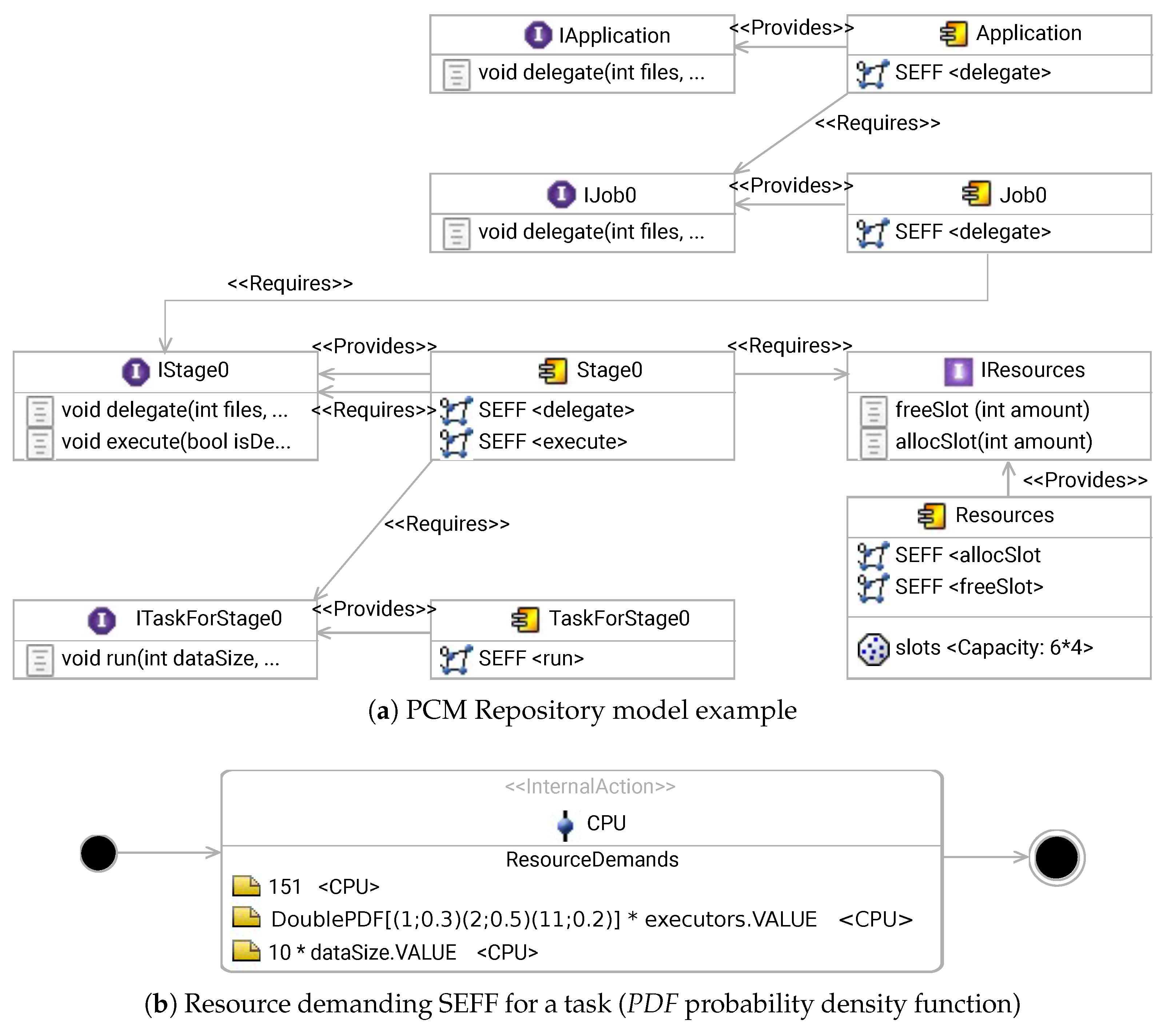
5. Transformation to Performance Models

This section describes the concepts of the architecture-level performance model PCM and how we transform DSL instances into PCM models.

5.1. Palladio Component Model

We chose to use PCM [6] as a model-based performance evaluation tool as it enables engineers to specify software systems independent of technology, include resource demands for software components, consider resource contention, and predict not only response time, but also resource utilization. Furthermore, the tool support is mature, open source, and continuously maintained with a large community.
In particular, PCM is developed for component-based software systems and enables engineers to describe performance relevant factors of software architectures, resource environments, and usage behavior [4]. It is implemented in Ecore from the Eclipse Modeling Framework (EMF) and consists of multiple models [6]. Software interfaces and components are specified in the Repository Model (Figure 4a). Components provide the implementation for signatures of interfaces. Therefore, they contain a resource demanding service effect specification (RDSEFF) in which the activities such as parametric resource demands and external calls of signatures are modeled similar to activity diagrams (Figure 4b). Components are additionally assembled in a System Model. In the Resource Environment Model, network and hardware resources are specified such as processing resources (CPU, disk, and delay), processing rates, and scheduling policies. The Allocation Model allows for deploying assembled components from the System Model on resources from the Resource Environment Model. The usage and workload of software components are specified in the Usage Model. Finally, PCM provides a simulator for its models, which is based on a process-oriented discrete event simulation.

5.2. Transformation to PCM

We describe the transformation for each DSL component. Table 1 shows the mapping of DSL concepts to PCM elements. An Execution Architecture is transformed to a Repository Model (Figure 4a). In order to traverse the Edges and Nodes of an Execution Architecture, we use a recursive depth-first search. Upon visiting each Node, we check if it contains child Nodes and Edges. If this is the case, we again traverse this Node and the procedure repeats.
For each Node, we create one Interface with several signatures and a corresponding Basic Component that provides the signatures using an RDSEFF. If a Node contains child Nodes, we add a delegate signature to the corresponding Interface (i.e., IJob0). Additionally, the Basic Component requires the Interfaces of the child Nodes.
Parameters of the Configuration and parametric dependencies of the Execution Architecture are transformed into input parameters of each Signature. We consider parameters for the number of files, the data size of one file, the default partition size, the number of partitions, and the number of executors. In order to model and limit the maximum number of concurrent tasks, we separately specify an Infrastructure Component to represent a pool of available task slots. The component contains two SEFFs to acquire and to release a task slot. In order to finally execute a task, a slot must be acquired first. After task completion, the slot is released again. In the case of Apache Spark, the limiting number of task slots is the number of total cores.
Edges are represented in the RDSEFF of a Basic Component. Each delegate RDSEFF models the flow by using External Call Actions to invoke signatures of required Interfaces in the specified order (i.e., Job0 invokes the prepare signature of IStage0). In the course of this, the input parameters are forwarded and altered at specific points to model the data transmission factor t e of an Edge.
If a Node contains a Resource Profile, we transform it by creating several model elements. In order to call a group of tasks in parallel, we add two signatures to the corresponding Interface of the Node (i.e., Stage0). The providing RDSEFF prepare is intended to create a set of parallel tasks. It uses a Distributed Call Action to invoke the execute signature of the same Interface several times in parallel. The parallelism is either defined by the number of partitions of a data source p d s or the specified parallelism of the Node p n . The execute RDSEFF acquires and releases a task slot before and after prompting a task.
We create an additional Interface and Basic Component (i.e., TaskForStage) to model a task. Its behavior run is responsible to execute the parametric resource demands of a task (Figure 4b). Only the wait demand of a Resource Profile will be executed in the prior prepare RDSEFF as the demand occurs once at the beginning of each stage and not for each task. We automatically assemble all Basic Components of the Repository Model in order to derive Palladio’s System Model.
Since the Resource Architecture follows the concepts of Palladio’s Resource Environment Model, the transformation is linear. We transform each Resource Node to a Resource Container and convert the Cluster Specification and Resource Role accordingly. Additionally, we transform each Resource Unit to an equivalent Processing Resource Unit including the specification of processing rates, number of replicas (e.g., the number of cores), and scheduling policies. Finally, all Resource Containers are connected to networks via a Linking Resource.
In order to create the Allocation Model, we deploy all assembled Basic Components from the System Model on the master Resource Container from the Resource Environment Model. Our previous extensions [9] enable Palladio’s simulation framework SimuCom to distribute resource demands to Resource Containers that represent worker nodes with a round robin policy.
Finally, we transform the Data Workload Architecture to a Usage Model. We create one Entry Level System Call that invokes the delegate signature of the Application Interface. The required input parameters are transformed based on the Data Model and Data Source. We specify the number of files, the data size of one file, the default partition size, and the number of partitions. For the Single Data Source, we create a simple closed Workload with a population of one, which means the Entry Level System Call is triggered once.
All transformed models can be used by Palladio’s simulator to predict performance metrics.

6. Evaluation

This section evaluates the model extraction and performance simulation approach introduced in this work.

6.1. Research Methodology

In order to validate our approach, we conduct three integrated controlled experiments by modeling and simulating the execution of two different exemplary machine learning applications [40]. Therefore, we formulate three claims by exemplary problems from a performance management perspective.
First, engineers are interested in the performance behavior of applications and resources in case data workload grows. This experiment evaluates the claim that data workloads can be changed independently of Execution Architectures and Resource Architectures. We initially extract one PerTract-DSL instance for each of the two applications based on monitoring data. Afterwards, we adapt data sizes in Data Workload Architectures and compare predictions for response times and CPU utilization with corresponding monitored measurements in several upscaling scenarios.
Second, engineers need to evaluate the scalability of applications if additional hardware resources are allocated. This experiment evaluates the claim that resources can be altered independently of Execution Architectures and Resource Architectures. We modify and add worker nodes in Resource Architectures without changing Execution Architectures and Data Workload Architectures. Afterwards, we compare predictions results with corresponding monitored measurements.
Third, engineers need to efficiently plan and manage capacities for given data workloads and performance requirements [5]. This experiment evaluates the claim that data workloads as well as resources can be changed independently of Execution Architectures. Similarly, we use the models extracted in the first experiment and conduct several upscaling scenarios regarding data workload and cluster size without modifying Execution Architectures. Afterwards, we compare the simulated prediction results with corresponding measurements.

6.2. HiBench Benchmark Suite

In our experiments, we apply the HiBench benchmark suite to run representative and reproducible applications and workloads for Apache Spark [41]. As the automatic extraction approach shall allow for modeling complex applications, we use two machine learning applications. We chose a random forest classification (RFC) since random forests represent frequently used machine learning models for classification and regression. HiBench implemented the application using Apache Spark’s machine learning library MLlib and provides an RFC-specific data generator. Additionally, we chose a linear regression (LR) as it is a common approach for regression analysis and forecasting. Therefore, HiBench’s implementation uses a model without regularization using a stochastic gradient descent to predict label values. Similarly, it implements Spark’s MLlib and includes its own data generator.

6.3. Experiment Setup

Table 2 and Table 3 illustrates our testbed and data configurations. The hardware environment includes five servers. Each server is connected to a storage area network (IBM System Storage EXP3512, New York, NY, USA) via fibre channel allowing for eight gigabits per second (GBit/s). The servers are also connected in a local area network (LAN) with one GBit/s.
We virtualized each server using the VMware ESXi hypervisor (VMware, Palo Alto, CA, USA) and configured eight cores and 36-gigabyte (GB) memory for each virtualized machine (VM). On each server, we allocated four VMs. On the first server, we use one VM as a master node for Apache HDFS and YARN, one VM for managing the cluster (i.e., Apache Ambari), one VM for storing monitoring data, and one VM for initiating the benchmark applications. On the remaining four servers, we use each VM as a worker node. We deployed the Hortonworks Data Platform to use Apache Spark, YARN, and HDFS. For HDFS, we kept the default configurations including a replication factor of three and a data block size of 128 megabytes (MB). For YARN, we configured 26 GB and six virtual cores (vCores) per container, for Spark executors 22 GB as well as six cores. Since we experienced that not all cores were utilized when running applications, we changed the resource calculator to be dominant and enabled CPU scheduling to address this issue. For evaluating the prediction accuracy, we compare the metrics response time and CPU utilization. For simulations, we captured the simulated mean response time (MRT) as well as the simulated mean CPU utilization (MCPU) across the cluster. For the benchmark measurements, applications were executed four times for each experiment to avoid any distortions. Similarly, monitored MRT and monitored MCPU on the user-level were calculated. Monitored response times are derived from the Spark monitoring API and monitored CPU measurements from the Ambari Metrics System (2.6.0).
Table 4 and Table 5 list all simulated and monitored MRT and MCPU results, the root mean square errors (RMSE), and the relative prediction errors. They provide the basis for presenting and discussing our experiments in the following.

6.4. Collecting Resource Demands and Extracting Execution Architectures

The extraction and transformation process follows the overview illustrated in Figure 1. In order to extract an Execution Architecture for one application, we monitor the application using our profiler presented in Section 4.1 to extract stack traces and corresponding CPU times. Additionally, the Spark framework itself monitors an application. As described in Section 4.2, execution components and inter-component interactions are extracted using Spark’s interfaces. For each execution component, CPU resource demands are generated by processing corresponding CPU times and interrelating them with data input information of each component as explained in Section 4.3.
In order to evaluate the three proposed claims, we derive one initial PerTract-DSL instance for each of the two machine learning applications that we use throughout all experiments. According to each experiment and scenario, we adapt the PerTract-DSL instance and simulate it to derive predictions.

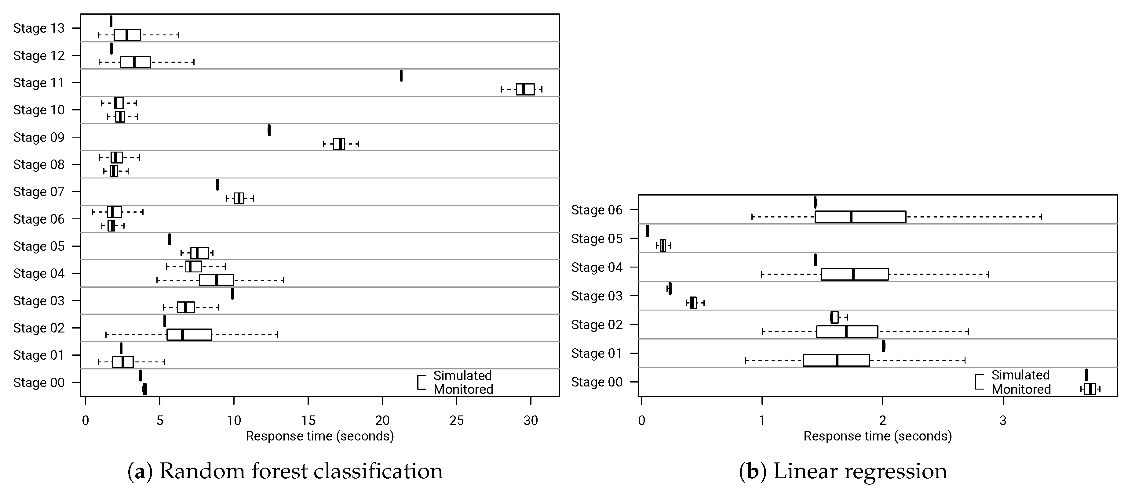
6.5. Evaluating Data Workload Changes

In order to evaluate our first claim that data workload changes can be modified independently, we specified three different scenarios small, large, and huge for both applications. Table 3 shows the corresponding number of files, file sizes, total partitions and total sizes for each scenario. The basis for evaluating workload changes of each application provides one initial PerTract-DSL instance each. We extracted this instance from a monitored experiment with a small data workload in a cluster of four worker nodes. Afterwards, we changed the Data Workload Architecture according to the scenarios large and huge and simulated the model instances. The simulation and monitoring results are part of Table 4 and Table 5.
The starting experiment (i.e., four nodes and small workload) shows a response time prediction error of 0.78% for the RFC and 2.23% for the LR application. CPU prediction errors amount to 6.69% and 2.94%. Changing the data workload according to the large and huge scenarios leads to a response time prediction error of 7.90% and 7.73% for the RFC and 6.45% and 6.30% for the LR applications. Similar to the prediction errors, the RMSE increased in both scenarios. For the huge scenario, Figure 5 illustrates the response time statistics of simulated and monitored Spark tasks for each stage. For both applications, we predict the median of the tasks for 16 of 21 stages with errors below 30%. However, the monitored results show an increased deviation compared to the simulation results, especially, for the LR application. This is due to the monitored delays and task processing, which showed great variances. While we model delays with probability distributions, we only use the mean for estimating CPU demands and did not depict this behavior. For the RFC application, tasks for stages 05, 07, 09, and 11 also differ significantly. These stages contain reduce operations for which the input data size does not exactly scale linearly with increasing data workload for this RFC application. However, the error only has a minor effect on the overall application response time as stages for reduce tasks consist of only eight tasks compared to 360 tasks for each of the other stages.
For the large and huge workload scenarios, the RMSE for CPU consistently remain below 9%. CPU prediction errors amount to 14.45% and 11.42% for the RFC and 9.53% and 1.54% for the LR application. Figure 6 illustrates the CPU utilization over time for one experiment run. In order to avoid illustrating too many lines, we calculated the mean across the worker nodes. Although underestimating the CPU utilization by 6.4% for the RFC application, the graphs of the simulated and monitored values map very closely.
The results for response time and resource utilization show accurate prediction results based upon averages for upscaling workload changes. Therefore, we validated the claim of being able to change data workloads independent of Execution Architectures and Resource Architectures.

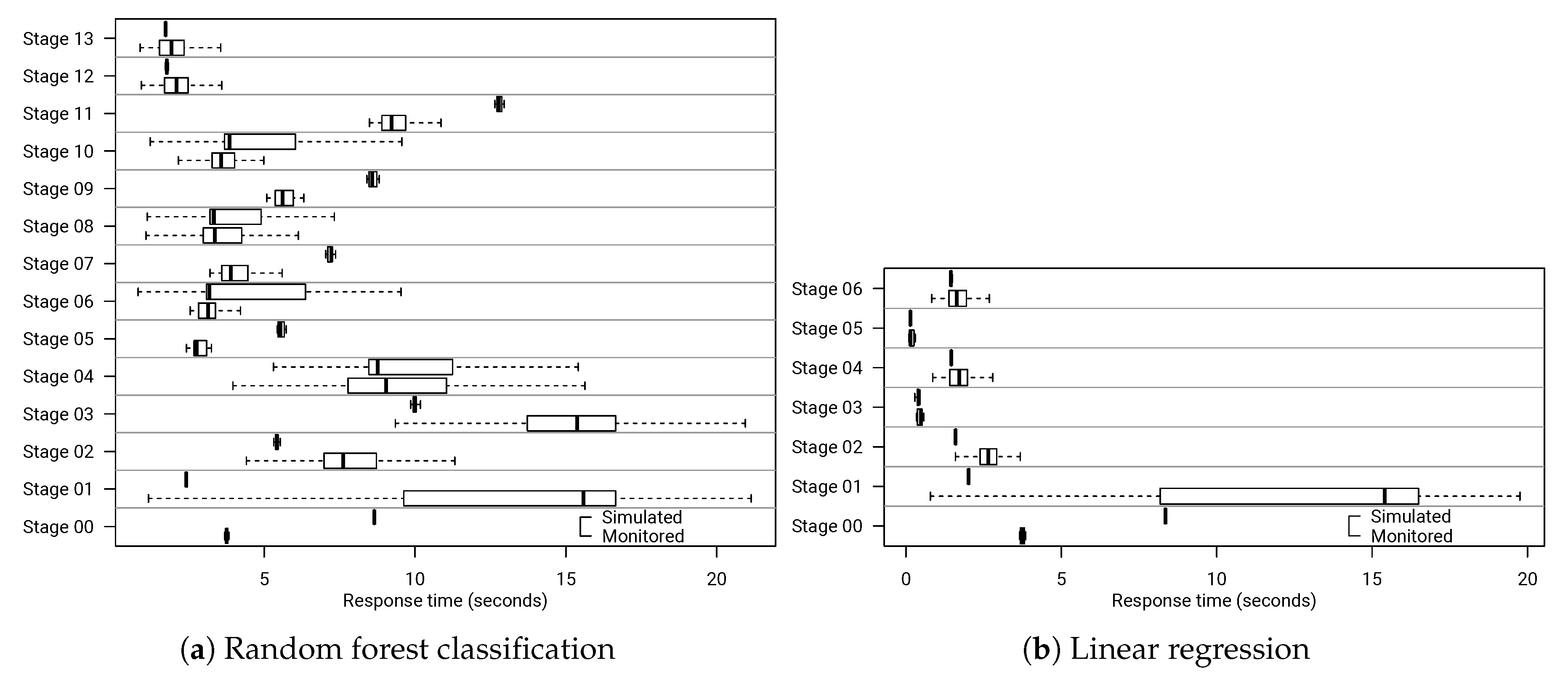
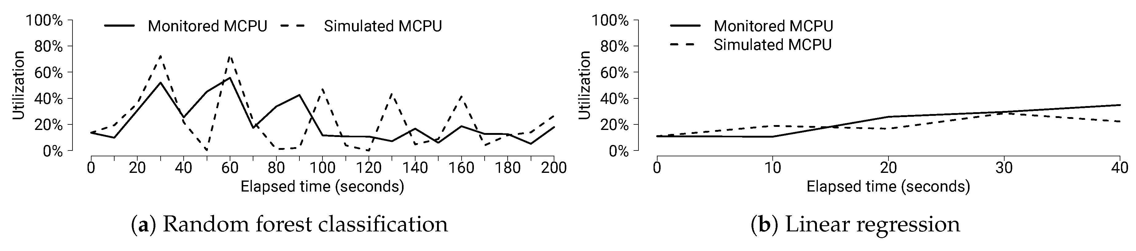
6.6. Evaluating Resource Changes

We increased the initial cluster size of four worker nodes by factors two and four in order to evaluate our second claim that hardware resources can be changed independently of Execution Architectures and Data Workload Architectures.
Similarly, the evaluation is based on one initial PerTract-DSL instance for each application, which is the same as for the data workload evaluation and was extracted from a monitored experiment with four worker nodes. Afterwards, we increased the worker nodes to eight and 16 nodes in the Resource Architecture. Additionally, we adapted the number of executors e in the application configuration of the Execution Architecture to match the number of worker nodes. The simulation and monitoring results are part of Table 4 and Table 5.
In the previous subsection, we already discussed the same starting experiment, which does not include any changes. For eight worker and 16 worker nodes, response time prediction errors amount to 10.53% and 0.08% for the RFC application and 6.59% and 1.34% for the LR application, respectively. Compared to the data workload changes, the RMSE is lower throughout the resource changes for both applications. Figure 7 additionally shows the detailed response time statistics of Spark tasks for each stage of the applications. Compared to the data workload evaluation, the median values of simulated and monitored results lie closer together. The distance of the first and third quartiles are also predicted more accurately for most stages of both applications. For a few stages such as Stage 01, minimum, maximum, and quartiles differ significantly. Nonetheless, response time predictions errors on application-level remain below 15% in total.
For eight worker and 16 worker nodes, CPU prediction errors come to 1.13% and 2.32% for the RFC application and to 9.86% and 12.26% for the LR application, respectively. Figure 8 illustrates the CPU utilization over time for one experiment run. For the RFC application, the simulated CPU usage overestimates several peaks and underestimates negative peaks. However, it depicts the progression of the monitored results overall. For the LR application, the predicted CPU utilization is very precise.
In total, the simulation results show accurate prediction results for upscaling hardware resource changes with mean prediction errors below 15% and validate the claim that hardware resource can be modified without changing Execution Architectures and Data Workload Architectures.

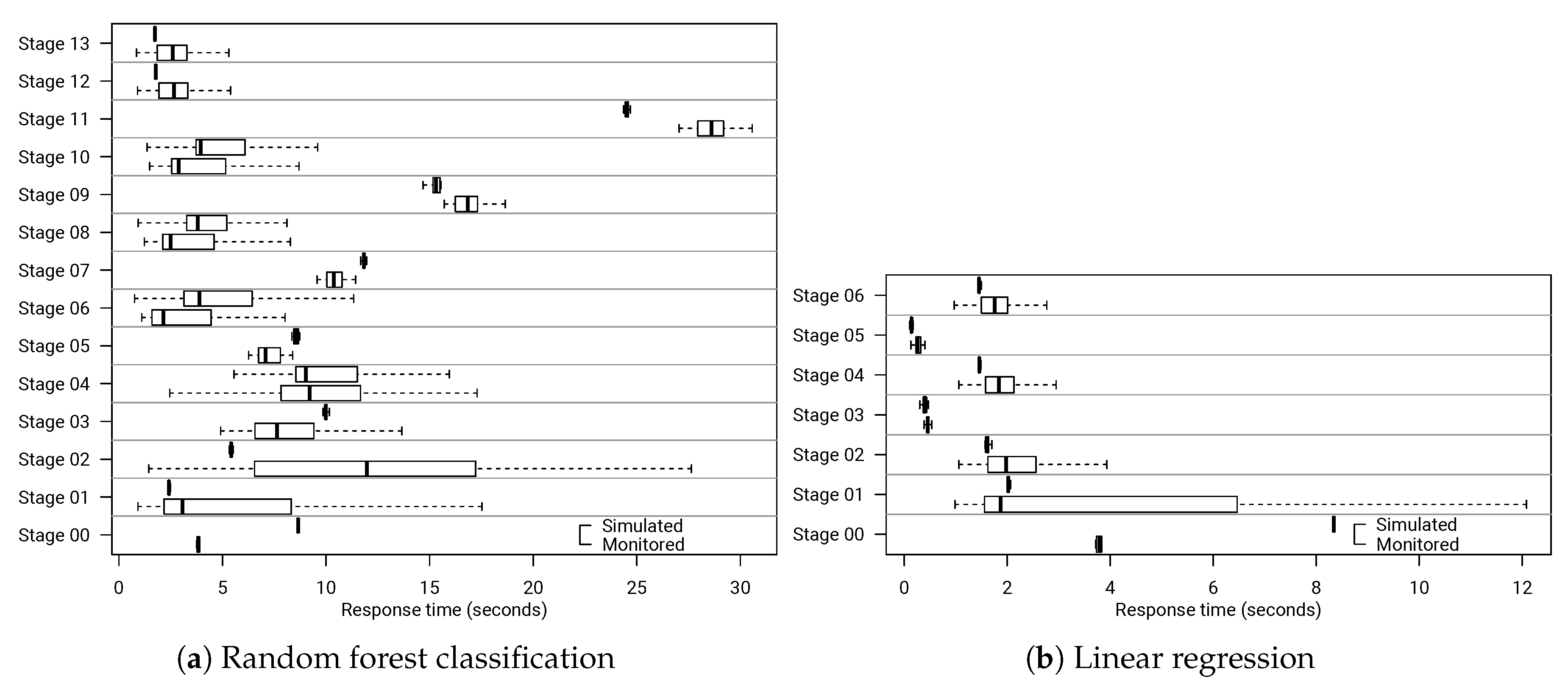
6.7. Evaluating Data Workload and Resource Changes

In order to evaluate our claim that data workload and hardware resources can be modified without changing application Execution Architectures, we applied both upscaling scenarios together, regarding data workload as well as worker nodes. The simulation and monitoring results are part of Table 4 and Table 5. Again, the evaluation is based on the same initially extracted PerTract-DSL instance for each application.
For eight worker nodes and a large data workload, response time prediction errors amount to 14.74% for the RFC and 4.79% for the LR application. For huge data workload, the errors are 8.94% and 4.15%, respectively. For 16 worker nodes and a large data workload, response time prediction errors come to 0.76% for the RFC and 10.74% for the LR application. With huge data workload, the errors are 6.06% and 6.93%, respectively. The RMSE results consistently behave similarly to prediction errors. The highest RMSE amounts to 56.62 s, which equals 14.97% of the corresponding monitored response times. For all scenarios, prediction errors constantly remain below 15%. Figure 9 additionally shows the response time statistics of results with 16 worker nodes and huge workload. Compared to the two previous evaluations, the simulation results depict monitoring results as the closest for both applications.
Looking at the CPU results for eight worker nodes and a large data workload, prediction errors amount to 11.29% for the RFC application and 7.85% for the LR application. For a huge workload, the errors remain similarly with 13.98% and 9.04%. For 16 worker nodes and a large data workload, the errors also remain 11.57% and 8.97%. With a huge data workload, they decrease a little to 9.63% and 6.89%, similar to the response time prediction.
Figure 10 shows the CPU utilization over time of one run with 16 worker nodes and a huge data workload. In case of the RFC application, the simulation graph depicts the progression of the monitored measurements. However, it shifts as the response time differs. In case of the LR application, the simulated CPU utilization is also slightly shifted due to the different response times. Otherwise, it depicts the monitored utilization except for one peak at the beginning. This is due to overestimating the CPU demand for Stage 00. Similarly, the task response time also significantly differs for Stage 00 for both applications throughout all experiments. The reason for the overestimation is that this stage consists of only one task, which does not scale linearly with the dependent data size. This is a case that we intentionally did not consider and could not cover as it requires metaknowledge of the application that we do not expect in an automatic extraction process.
Overall, the simulated results for response times on an application-level as well as CPU utilization show accurate predictions for both data workload changes and hardware resources. The mean prediction errors remained below 15% as well as the RMSE compared to the monitored results. In performance evaluation literature, prediction errors of 30% across cluster sizes are expected [20]. Therefore, we validated the claim of being able to change data workloads and resources’ architectures independent of Execution Architectures. Our approach enriches related work by predicting CPU utilization across clusters and over time.

6.8. Threats to Validity

Although we applied some sophisticated machine learning applications, we generated data and used only a set of sample applications from one benchmark suite. As they are far more complex applications and have deviating data in praxis, this represents a threat to external validity [42].
Furthermore, we evaluated our approach only for one technology (i.e., Apache Spark) and one type of application (i.e., batch). In previous work, we showed that our approach is also applicable for Spark Streaming applications [11]. However, we claim that the DSL builds a foundation to specify other technologies as well, such as Apache Flink and Apache Storm. Extensions might be required (e.g., additional parameters) to support modeling and accurate predictions. We plan to evaluate this in our future work.
We used several visualizations and statistical measures such as mean, standard deviation, and relative error to ensure statistical conclusion validity. While the results of one measure can be close to each other (e.g., mean), another measure can differ significantly (e.g., minimum value).

6.9. Assumptions and Limitations

We allocated one Spark executor to each node during our experiments. It is also possible to size less cores and memory for Spark executors, which would enable Spark to allocate multiple executors to one node. Although we are also able to model and simulate these scenarios, we did not evaluate such a case. We evaluated our experiments in a virtualized, but exclusive cluster in which no other applications were running in parallel and using any CPU, disk drives, or networks. For data analytics applications, CPU is usually the bottleneck [37]. As HiBench and other industry benchmarks mainly consist of only compute-intensive applications, we did not evaluate our approach for a wider variety of applications.
Regarding our modeling approach, we specified the input of a subsequent Spark stage probabilistically depending on the output data of a previous stage. Therefore, our prediction error will increase, if the properties of the initial underlying data set change significantly (e.g., the number of distinct words in case of a word count application). Another limitation is that we only include network delays in our models and simulations, but did not simulate network throughput and bandwidth yet. The same applies to disk drives. In addition, we also did not consider rack awareness in our specification. Regarding big data features and PCM, Heinrich et al. [43] discuss current challenges and potential solutions, for instance, for modeling data structures and continuous data flows.

7. Conclusions and Future Work

Modeling and predicting the performance of big data applications are essential for planning capacities and evaluating configurations. Automatically deriving models, specifying applications tool-agnostic, and gaining insights into performance-relevant factors of system architectures and dependencies are complex challenges. We present PerTract, an approach to automatically extract model specifications and transform them to the model-based performance evaluation tool Palladio. A PerTract-DSL allows the specification of (i) application execution architectures including components, parametric dependencies, and resource demands, (ii) computing resources, and (iii) data workloads. It is specifically designed for big data systems, decreases the complexity compared to full performance models, and simplifies the changeability to users. We demonstrated the extraction of DSL instances by the example of Apache Spark applications, Apache YARN resources, and Apache HDFS data. This is the first white-box approach to present an automated way to integrate measurements and estimate resource demands to produce performance models that can be simulated. We used two machine learning applications of the HiBench benchmark suite in the evaluation and upscaled data sizes as well as cluster sizes in different scenarios. We are able to predict mean response times on application-level and CPU usage with accurate predictions errors below 15%.
In our future work, we plan to extract DSL instances from more technologies. We already provide a way to extract the execution architecture of Apache Flink applications, but need further investigations to estimate accurate resource demands. Additional technologies include Apache Mesos for modeling computing resources and Apache Kafka for characterizing data workload. We also plan to implement direct transformations from the DSL to a scalable event-oriented discrete-event simulation as we are reaching the limit for simulating continuous sources (data streams). Finally, we will extend the specification of continuous data sources to include load intensity profiles that model variations in arrival rates [44].

Author Contributions

Conceptualization: J.K. and H.K.; Resources: H.K.; Software: J.K.; Validation: J.K.; Writing—original draft: J.K.; Writing—review and editing: J.K. and H.K.; Supervision: H.K.

Funding

This research received no external funding.

Conflicts of Interest

The authors declare no conflict of interest.

Abbreviations

The following abbreviations are used in this manuscript:
CPUCentral processing unit
DSLDomain-specific language
EMFEclipse modeling framework
GBGigabyte
HDFSHadoop distributed file system
LANLocal area network
LRLinear regression
MBMegabytes
MCPUMean CPU utilization
MRTMean response time
PCMPalladio component model
PDFProbability density function
RDDResilient distributed dataset
RDSEFFResource demanding service effect specification
RFCRandom forest classification
RMSERoot mean square error
VMVirtualized machine

References

  1. Schermann, M.; Hemsen, H.; Buchmüller, C.; Bitter, T.; Krcmar, H.; Markl, V.; Hoeren, T. Big Data—An interdisciplinary opportunity for information systems research. Bus. Inf. Syst. Eng. 2014, 6, 261–266. [Google Scholar] [CrossRef]
  2. Brunnert, A.; Vögele, C.; Danciu, A.; Pfaff, M.; Mayer, M.; Krcmar, H. Performance management work. Bus. Inf. Syst. Eng. 2014, 6, 177–179. [Google Scholar] [CrossRef]
  3. Wang, K.; Khan, M.M.H. Performance Prediction for Apache Spark Platform. In Proceedings of the 17th International Conference on High Performance Computing and Communications, New York, NY, USA, 24–26 August 2015; pp. 166–173. [Google Scholar]
  4. Brosig, F.; Meier, P.; Becker, S.; Koziolek, A.; Koziolek, H.; Kounev, S. Quantitative Evaluation of Model-Driven Performance Analysis and Simulation of Component-Based Architectures. IEEE Trans. Softw. Eng. 2015, 41, 157–175. [Google Scholar] [CrossRef]
  5. Brunnert, A.; van Hoorn, A.; Willnecker, F.; Danciu, A.; Hasselbring, W.; Heger, C.; Herbst, N.; Jamshidi, P.; Jung, R.; von Kistowski, J.; et al. Performance-Oriented DevOps: A Research Agenda; Technical Report SPEC-RG-2015-01; SPEC Research Group—DevOps Performance Working Group, Standard Performance Evaluation Corporation (SPEC): Gainesville, FL, USA, 2015; Available online: http://research.spec.org/fileadmin/user_upload/documents/wg_devops/endorsed_publications/SPEC-RG-2015-001-DevOpsPerformanceResearchAgenda.pdf (accessed on 8 August 2019).
  6. Becker, S.; Koziolek, H.; Reussner, R. The Palladio component model for model-driven performance prediction. J. Syst. Softw. 2009, 82, 3–22. [Google Scholar] [CrossRef]
  7. Kroß, J. PerTract. Available online: https://github.com/johanneskross/pertract (accessed on 7 August 2019).
  8. Kroß, J.; Brunnert, A.; Prehofer, C.; Runkler, T.; Krcmar, H. Stream Processing on Demand for Lambda Architectures. In Computer Performance Engineering; Beltrán, M., Knottenbelt, W., Bradley, J., Eds.; Lecture Notes in Computer Science; Springer International Publishing: Cham, Switzerland, 2015; Volume 9272, pp. 243–257. [Google Scholar]
  9. Kroß, J.; Brunnert, A.; Krcmar, H. Modeling Big Data Systems by Extending the Palladio Component Model. In Proceedings of the 2015 Symposium on Software Performance, Munich, Germany, 4–6 November 2015. [Google Scholar]
  10. Kroß, J.; Krcmar, H. Modeling and Simulating Apache Spark Streaming Applications. In Proceedings of the 2016 Symposium on Software Performance, Kiel, Germany, 8–9 November 2016. [Google Scholar]
  11. Kroß, J.; Krcmar, H. Model-based Performance Evaluation of Batch and Stream Applications for Big Data. In Proceedings of the IEEE 25th International Symposium on Modeling, Analysis and Simulation of Computer and Telecommunication Systems (MASCOTS), Banff, AB, Canada, 20–22 September 2017; pp. 80–86. [Google Scholar]
  12. Vianna, E.; Comarela, G.; Pontes, T.; Almeida, J.; Almeida, V.; Wilkinson, K.; Kuno, H.; Dayal, U. Analytical Performance Models for MapReduce Workloads. Int. J. Parallel Program. 2013, 41, 495–525. [Google Scholar] [CrossRef]
  13. Verma, A.; Cherkasova, L.; Campbell, R.H. Profiling and evaluating hardware choices for MapReduce environments: An application-aware approach. Perform. Eval. 2014, 79, 328–344. [Google Scholar] [CrossRef]
  14. Zhang, Z.; Cherkasova, L.; Loo, B.T. Benchmarking Approach for Designing a Mapreduce Performance Model. In Proceedings of the ACM/SPEC International Conference on Performance Engineering, Prague, Czech Republic, 21–24 April 2013; ACM Press: New York, NY, USA, 2013; pp. 253–258. [Google Scholar]
  15. Zhang, Z.; Cherkasova, L.; Loo, B.T. Performance Modeling of MapReduce Jobs in Heterogeneous Cloud Environments. In Proceedings of the 2013 IEEE Sixth International Conference on Cloud Computing, Santa Clara, CA, USA, 28 June–3 July 2013; IEEE: Washington, DC, USA, 2013; pp. 839–846. [Google Scholar] [Green Version]
  16. Zhang, Z.; Cherkasova, L.; Loo, B.T. Exploiting Cloud Heterogeneity to Optimize Performance and Cost of MapReduce Processing. SIGMETRICS Perform. Eval. Rev. 2015, 42, 38–50. [Google Scholar] [CrossRef]
  17. Barbierato, E.; Gribaudo, M.; Iacono, M. Performance evaluation of NoSQL big-data applications using multi-formalism models. Future Gener. Comput. Syst. 2014, 37, 345–353. [Google Scholar] [CrossRef]
  18. Ardagna, D.; Bernardi, S.; Gianniti, E.; Karimian Aliabadi, S.; Perez-Palacin, D.; Requeno, J.I. Modeling Performance of Hadoop Applications: A Journey from Queueing Networks to Stochastic Well Formed Nets. In Algorithms and Architectures for Parallel Processing; Carretero, J., Garcia-Blas, J., Ko, R.K., Mueller, P., Nakano, K., Eds.; Lecture Notes in Computer Science; Springer International Publishing: Cham, Switzerland, 2016; pp. 599–613. [Google Scholar] [Green Version]
  19. Lehrig, S. Applying Architectural Templates for Design-Time Scalability and Elasticity Analyses of SaaS Applications. In Proceedings of the 2nd International Workshop on Hot Topics in Cloud Service Scalability, Dublin, Ireland, 22 March 2014; pp. 2:1–2:8. [Google Scholar]
  20. Ardagna, D.; Barbierato, E.; Evangelinou, A.; Gianniti, E.; Gribaudo, M.; Pinto, T.B.M.; Guimarães, A.; da Silva, A.P.C.; Almeida, J.M. Performance Prediction of Cloud-Based Big Data Applications. In Proceedings of the ACM/SPEC International Conference on Performance Engineering, Berlin, Germany, 9–13 April 2018; pp. 192–199. [Google Scholar]
  21. Singhal, R.; Singh, P. Performance Assurance Model for Applications on SPARK Platform. In Performance Evaluation and Benchmarking for the Analytics Era; Nambiar, R., Poess, M., Eds.; Lecture Notes in Computer Science; Springer International Publishing: Cham, Switzerland, 2018; pp. 131–146. [Google Scholar]
  22. Venkataraman, S.; Yang, Z.; Franklin, M.; Recht, B.; Stoica, I. Ernest: Efficient Performance Prediction for Large-Scale Advanced Analytics. In Proceedings of the 13th USENIX Symposium on Networked Systems Design and Implementation (NSDI 16), Santa Clara, CA, USA, 13–17 March 2016; USENIX Association: Santa Clara, CA, USA, 2016; pp. 363–378. [Google Scholar]
  23. Alipourfard, O.; Liu, H.H.; Chen, J.; Venkataraman, S.; Yum, M.; Zhang, M. CherryPick: Adaptively Unearthing the Best Cloud Configurations for Big Data Analytics. In Proceedings of the 14th USENIX Symposium on Networked Systems Design and Implementation (NSDI 17), Boston, MA, USA, 27–29 March 2017; USENIX Association: Boston, MA, USA, 2017; pp. 469–482. [Google Scholar]
  24. Witt, C.; Bux, M.; Gusew, W.; Leser, U. Predictive performance modeling for distributed batch processing using black box monitoring and machine learning. Inf. Syst. 2019, 82, 33–52. [Google Scholar] [CrossRef] [Green Version]
  25. Castiglione, A.; Gribaudo, M.; Iacono, M.; Palmieri, F. Modeling performances of concurrent big data applications. Softw. Pract. Exp. 2014, 45, 1127–1144. [Google Scholar] [CrossRef]
  26. Niemann, R. Towards the Prediction of the Performance and Energy Efficiency of Distributed Data Management Systems. In Proceedings of the ACM/SPEC International Conference on Performance Engineering, Delft, The Netherlands, 12–16 March 2016; pp. 23–28. [Google Scholar]
  27. Casale, G.; Ardagna, D.; Artac, M.; Barbier, F.; Nitto, E.D.; Henry, A.; Iuhasz, G.; Joubert, C.; Merseguer, J.; Munteanu, V.I.; et al. DICE: Quality-driven Development of Data-intensive Cloud Applications. In Proceedings of the Seventh International Workshop on Modeling in Software Engineering, Florence, Italy, 16–24 May 2015; pp. 78–83. [Google Scholar]
  28. Guerriero, M.; Tajfar, S.; Tamburri, D.A.; Di Nitto, E. Towards a Model-driven Design Tool for Big Data Architectures. In Proceedings of the 2nd International Workshop on BIG Data Software Engineering, Austin, TX, USA, 2016; pp. 37–43. [Google Scholar]
  29. Gómez, A.; Merseguer, J.; Di Nitto, E.; Tamburri, D.A. Towards a UML Profile for Data Intensive Applications. In Proceedings of the 2Nd International Workshop on Quality-Aware DevOps, Saarbrücken, Germany, 21 July 2016; pp. 18–23. [Google Scholar]
  30. Ginis, R.; Strom, R.E. Method for Predicting Performance of Distributed Stream Processing Systems. U.S. Patent 7,818,417, 19 October 2010. [Google Scholar]
  31. Steinberg, D.; Budinsky, F.; Paternostro, M.; Merks, E. EMF: Eclipse Modeling Framework, 2nd ed.; Addison-Wesley: Boston, MA, USA, 2009. [Google Scholar]
  32. King, B. Performance Assurance for IT Systems; Auerbach Publications: Boston, MA, USA, 2004. [Google Scholar]
  33. Brandl, R.; Bichler, M.; Ströbel, M. Cost accounting for shared IT infrastructures. Wirtschaftsinformatik 2007, 49, 83–94. [Google Scholar] [CrossRef]
  34. Brunnert, A.; Krcmar, H. Continuous Performance Evaluation and Capacity Planning Using Resource Profiles for Enterprise Applications. J. Syst. Softw. 2017, 123, 239–262. [Google Scholar] [CrossRef]
  35. Zaharia, M.; Chowdhury, M.; Das, T.; Dave, A.; Ma, J.; McCauley, M.; Franklin, M.J.; Shenker, S.; Stoica, I. Resilient Distributed Datasets: A Fault-tolerant Abstraction for In-memory Cluster Computing. In Proceedings of the 9th USENIX Conference on Networked Systems Design and Implementation, San Jose, CA, USA, 25–27 April 2012; USENIX Association: Berkeley, CA, USA, 2012; p. 2. [Google Scholar]
  36. Apache Spark. Lightning-Fast Cluster Computing. Available online: https://spark.apache.org (accessed on 19 February 2018).
  37. Ousterhout, K.; Rasti, R.; Ratnasamy, S.; Shenker, S.; Chun, B.G. Making Sense of Performance in Data Analytics Frameworks. In Proceedings of the 12th USENIX Symposium on Networked Systems Design and Implementation, Oakland, CA, USA, 4–6 May 2015; USENIX Association: Oakland, CA, USA, 2015; pp. 293–307. [Google Scholar]
  38. Apache Hadoop. Welcome to Apache Hadoop! Available online: https://hadoop.apache.org/ (accessed on 1 January 2017).
  39. Dean, J.; Ghemawat, S. MapReduce: Simplified Data Processing on Large Clusters. Commun. ACM 2008, 51, 107–113. [Google Scholar] [CrossRef]
  40. Hevner, A.R.; March, S.T.; Park, J.; Ram, S. Design Science in Information Systems Research. MIS Q. 2004, 28, 75–105. [Google Scholar] [CrossRef]
  41. Huang, S.; Huang, J.; Dai, J.; Xie, T.; Huang, B. The HiBench benchmark suite: Characterization of the MapReduce-based data analysis. In Proceedings of the 26th International Conference on Data Engineering Workshops, Long Beach, CA, USA, 1–6 March 2010; pp. 41–51. [Google Scholar]
  42. Wohlin, C.; Runeson, P.; Höst, M.; Ohlsson, M.C.; Regnell, B.; Wesslén, A. Experimentation in Software Engineering; Springer: Berlin/Heidelberg, Germany, 2012. [Google Scholar]
  43. Heinrich, R.; Eichelberger, H.; Schmid, K. Performance Modeling in the Age of Big Data—Some Reflections on Current Limitations. In Proceedings of the 3rd International Workshop on Interplay of Model-Driven and Component-Based Software Engineering, Saint-Malo, France, 2 October 2016; pp. 37–38. [Google Scholar]
  44. Kistowski, J.V.; Herbst, N.; Kounev, S.; Groenda, H.; Stier, C.; Lehrig, S. Modeling and Extracting Load Intensity Profiles. ACM Trans. Auton. Adapt. Syst. 2017, 11, 23:1–23:28. [Google Scholar] [CrossRef]
Figure 1. Overview of the extraction and transformation approach.
Bdcc 03 00047 g001
Figure 2. Exemplary PerTract-DSL instance.
Bdcc 03 00047 g002
Figure 3. PerTract-DSL classes and relationships.
Bdcc 03 00047 g003
Figure 4. Exemplary transformed PCM instances.
Bdcc 03 00047 g004
Figure 5. Response time statistics of Spark tasks for each stage (four worker nodes, huge data workload).
Bdcc 03 00047 g005
Figure 6. Mean CPU utilization of four worker nodes (huge data workload).
Bdcc 03 00047 g006
Figure 7. Response time statistics of Spark tasks for each stage (16 worker nodes, small data workload).
Bdcc 03 00047 g007
Figure 8. Mean CPU utilization of 16 worker nodes (small data workload).
Bdcc 03 00047 g008
Figure 9. Response time statistics of Spark tasks for each stage (16 worker nodes, huge data workload).
Bdcc 03 00047 g009
Figure 10. Mean CPU utilization of 16 worker nodes (huge data workload).
Bdcc 03 00047 g010
Table 1. Mapping of PerTract-DSL to PCM elements.
PerTract-DSLPCM Model Elements
Execution ArchitectureRepository Model
 Nodes Interface, Basic Component
 Edges RDSEFF
 Configuration Parameters, Infrastructure Component
Resource Profile Distributed Call Action, RDSEFF
Resource ArchitectureResource Environment Model
 Resource Node Resource Container
 Cluster Specification Cluster Specification
 Network Channel Linking Resource
Data Workload ArchitectureUsage Model
 Data Model Entry Level SystemCall, Parameters
 Data Source Workload
RDSEFF Resource Demanding Service Effect Specification; Distributed Call Action, Cluster Specification PCM extensions [9].
Table 2. Software and hardware configuration of the test system.
Software platform Hortonworks Data Platform (2.6.3.0-235)
 - Apache Spark (2.2.0)
 - Apache Hadoop (2.7.3)
 - Apache Ambari (2.6.0)
Java virtual machine Oracle JDK (1.8.0_60)
Operating system CentOS Linux (7.2.1511)
Virtualization VMware ESXi (5.1.0), 8 cores, 36 GB RAM
CPU cores48 × 2.1 GHz
CPU sockets4 × AMD Opteron 6172
Random access memory (RAM)256 gigabyte (GB)
Hardware systemIBM System X3755M3
Table 3. Data workload scenarios and configurations.
ApplicationScenarioFile SizeFilesPartitionsTotal Size
Random forest classificationSmall1.89 gigabyte812815.12 gigabyte
Large3.58 gigabyte823228.64 gigabyte
Huge5.52 gigabyte836044.16 gigabyte
Linear regressionSmall1.86 gigabyte812014.88 gigabyte
Large3.49 gigabyte822427.92 gigabyte
Huge5.59 gigabyte836044.72 gigabyte
Table 4. Monitored and simulated mean response times (seconds).
Random Forest Classification ApplicationLinear Regression Application
WorkerDataMonitoredSimulated PredictionMonitoredSimulated Prediction
NodesWorkloadMRTMRTRMSEErrorMRTMRTRMSEError
4Small264.79262.714.470.78%42.1543.091.192.23%
Large502.09462.4140.267.90%71.9676.604.736.45%
Huge755.05696.7059.657.73%124.21116.3813.396.30%
8Small222.46199.0424,9210.53%35.2832.952.656.59%
Large378.31322.5456.6214.74%52.2449.743.664.79%
Huge534.12486.3448.488.94%76.7373.544.604.15%
16Small196.62196.464.340.08%37.8437.332.221.34%
Large287.38285.2011.560.76%40.8645.244.4810.74%
Huge373.74396.3825.976.06%53.2756.964.056.93%
Table 5. Monitored and simulated mean CPU utilization.
Random Forest Classification ApplicationLinear Regression Application
WorkerDataMonitoredSimulated PredictionMonitoredSimulated Prediction
NodesWorkloadMCPUMCPURMSEErrorMCPUMCPURMSEError
4Small48.96%45.69%3.31%6.69%48.86%47.43%2.53%2.94%
Large56.93%48.70%8.23%14.45%57.55%52.06%5.62%9.53%
Huge56.06%49.66%6.43%11.42%56.32%55.45%4.02%1.54%
8Small35.23%34.83%0.91%1,13%36.03%32.48%3.72%9.86%
Large44.64%39.60%5.31%11.29%46.13%42.51%3.85%7.85%
Huge47.27%40.66%6.61%13.98%52.93%48.15%4.81%9.04%
16Small22.65%22.12%0.84%2.32%22.05%19.34%2.91%12.26%
Large31.23%27.61%3.65%11.57%31.85%28.99%3.06%8.97%
Huge34.00%30.72%3.39%9.63%38.22%35.59%3.13%6.89%

