Data Stream Clustering Techniques, Applications, and Models: Comparative Analysis and Discussion

Abstract

Data growth in today’s world is exponential, many applications generate huge amount of data streams at very high speed such as smart grids, sensor networks, video surveillance, financial systems, medical science data, web click streams, network data, etc. In the case of traditional data mining, the data set is generally static in nature and available many times for processing and analysis. However, data stream mining has to satisfy constraints related to real-time response, bounded and limited memory, single-pass, and concept-drift detection. The main problem is identifying the hidden pattern and knowledge for understanding the context for identifying trends from continuous data streams. In this paper, various data stream methods and algorithms are reviewed and evaluated on standard synthetic data streams and real-life data streams. Density-micro clustering and density-grid-based clustering algorithms are discussed and comparative analysis in terms of various internal and external clustering evaluation methods is performed. It was observed that a single algorithm cannot satisfy all the performance measures. The performance of these data stream clustering algorithms is domain-specific and requires many parameters for density and noise thresholds.

1. Introduction

Nowadays automation is in almost every domain and transactions of everyday life are recorded at high speed. The huge amount of data generated by these processes can be termed a data stream. The problem of clustering data streams has been extensively studied and researched in recent years [1,2,3,4,5]. In many organizations, the number of transactions generated due to business process is very large; however, these transactions are recorded and kept, thus it is essential to analyze such data streams to extract trends for improvement in business development. As generation of records across business processes is a continuous process that occurs over time, the databases grow without limit. Such databases may show trend change over time, this process is data evolution.

In data mining, data objects are represented as points. The classification of data into clusters is unsupervised and can be denoted as $X= C_1 \cup \dots C_i \cup C_k; C_i \cap C_j= \mathsf{\Phi }\left(i \ne j\right)$ where, $X$ denotes original dataset, $C_i, C_j$ are clusters formed in $X$, and $k$ denotes the number of clusters formed [6]. In case of unsupervised knowledge, only former information of the domain and data are known, however structured characteristics are not known. It is very common that these unknown structural characteristics include the spatial distribution of the data. Characteristics such as volume, density, shape, or orientation are the basis of cluster formation. Clustering is a method to group unlabeled data sets based on “similarity” of the features extracted out of data items, and allocations of dissimilar data items in different groups. The clustering problem is to partition a given data set in one or more groups of similar objects. The similarity feature or measure of the objects with respect to each other is generally distance or density function. The traditional clustering techniques, methods, and algorithms are widely studied in the research community [7,8,9,10,11,12]. Recently, clustering with data streams and problems related to this are also discussed.

Most of the algorithms on clustering data streams generate clusters over the whole data set. These algorithms consider clustering as a single-pass clustering method. For some applications, such clustering methods are useful, however, in the case of data streams, it is necessary to define the clustering problem carefully, as the data stream is an infinite process in which data is evolved with time. The clusters are also varying with respect to the time when they are calculated and the time over which they are measured. For example, a particular application may have the requirement of the user to examine clustering occurring with respect to a time-frame, these clusters are attended as special case. Therefore, it is necessary for the data stream algorithm to provide an interface for user-defined time periods in order to generate relevant clusters. Various surveys have been conducted on mining data streams. Most of them discuss the techniques and theory related to data streams [2,13,14,15,16]. The most frequently used methods and techniques are discussed in some of the review literature [17,18]. Clustering algorithms are compared based on different characteristics [19]. Some of the review papers discuss density-based clustering techniques on data streams [20]. A survey in a past paper [21] discussed a review on density-based clustering techniques and methods for evolving data-streams. The work in a different paper [22] is one of the earlier contributions in survey of clustering algorithms. The authors have surveyed clustering algorithms used in different domains and their applications on benchmark datasets and computational problems. They also discussed many closely correlated topics such as cluster validation and proximity measures. The authors of a past paper [22] talked about applications, challenges, techniques, and technologies on big data. They have tried to present a list of technologies currently used to deal with big data. Their focus is on clustering techniques based on MapReduce and parallel classification using MapReduce. The authors of another past paper [22] used taxonomy and empirical analysis to survey clustering algorithms on big data. They presented a survey of different categories of existing clustering algorithms (partitioning-based, model-based, grid-based, hierarchical-based, and density-based). The authors give a comparison between these five categories of data clustering. The goal is to find the best performing algorithm for data stream clustering.

Motivation: In real-life applications some of the data set may contain large amounts of noise and outliers. Therefore clusters are not necessarily spherical in shape. The density-based clustering methods can handle noise and outliers effectively. It is not necessary to specify the number of clusters as initial assumptions. In many applications, the main issue is to do cluster analysis of evolving data streams. Some of the examples, where clustering of high dimensional data is very important, are described below.

Gene Expression Analysis: In the medical domain, a huge amount of data on molecular biology is being generated. This type of data (also called as gene expression data) consists of features such as gene expression. The gene expression level shows conclusions regarding the amount of the corresponding gene product. Such data comprises of concurrent measurement of the gene expression level for thousands of genes under hundreds of conditions. The data is represented in the form of a Data Matrix, in which rows are genes and columns are different experimental conditions, different tissues, consecutive time clots, or different patients. There exists a requirement for biologists to identify patterns within such bid datasets. Therefore, based on the scope of the research data mining tasks can be applied.

Text Documents: Generating clusters or groups based on themes from text documents, such as web pages, is necessary in many applications. In these cases, text documents are transformed into high-dimensional feature vectors based on frequency features. The data matrix generated contains rows and columns, where columns represent the count of one particular term. The documents are grouped based on the frequency of words and similar words in a subset of terms, these subsets are related to the theme of the documents. A particular document may happen to have overlap among groups for different themes; therefore it may be possible to assign membership of the document to various groups simultaneously, based on similarities of the frequency of words in the different subsets of terms.

Customer Recommendation Systems: In customer recommendation systems, reviews from the customers regarding a company’s product are captured. The company may have a wide range of products. Customer’s reviews having the same or similar remarks of preferences are grouped for market analysis. Based on the analysis special offers and strategic planning related to marketing is applied. The problem is to cluster customers with overlapping preferences based on the type of product.

The remainder of this paper is organized as follows. In the next section i.e., Section 2, traditional clustering techniques are discussed. In Section 3 one algorithm from each clustering technique is discussed that is related to data stream clustering. Section 4 overviews the criteria to evaluate clustering methods. Section 5 examines how algorithms overcome challenging issues and compare them based on evaluation metrics. In Section 6, experimentation and results are presented for some of these data stream clustering algorithms. Finally, Section 7 concludes our study and introduces some current issues in the clustering of data streams.

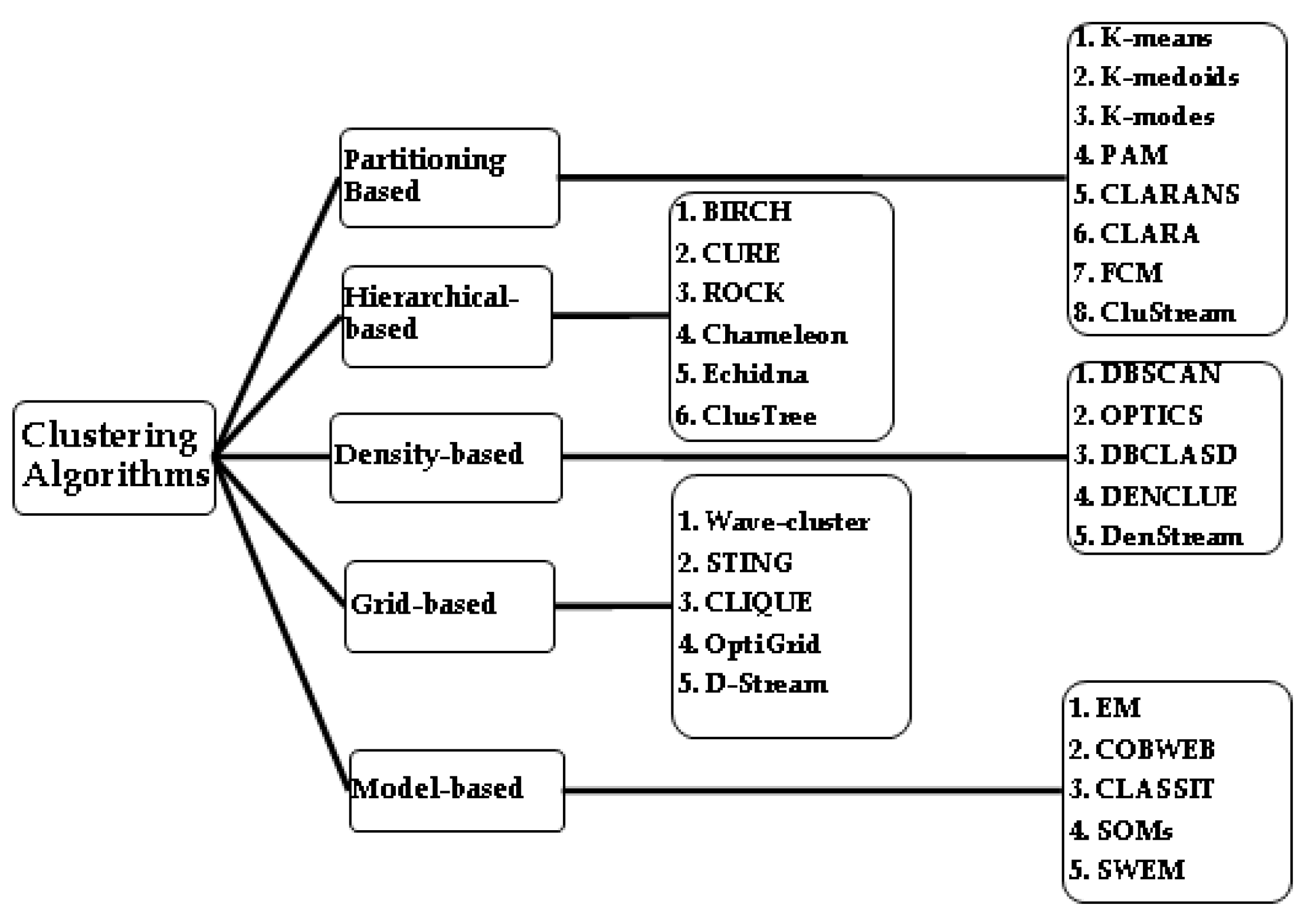
2. Clustering Techniques

A clustering technique is a process of grouping objects into different sets called clusters. Clustering is well-studied problem, and many clustering techniques have been proposed in past literature [23,24,25]. Data stream clustering typically maintains the synopsis of the data stream. Most of these algorithms are extended versions of traditional clustering algorithms satisfying certain constraints. The traditional clustering algorithms that are base-line algorithms for data stream algorithms are classified as follows.

2.1. Partitional Clustering

Partitioned-based methods mostly divide the data item (objects) sets into a number of groups called partitions, each partition represents a cluster. These clusters possess certain properties, e.g., each cluster must contain at least one data item and each data item should be categorized to exactly one cluster. There are many clustering methods using partition-based clustering algorithms such as K-means [26], K-medoids [6,27], K-modes [6,27], PAM [27], CLARA [27], CLARANS [27], FCM [27], and CluStream [1]. All of these algorithms generate clusters. In k-means clustering, a cluster is a group of points near to the center of the cluster. The k-medoids algorithm is similar to k-means but in the case of k-means the average distance is calculated; whereas, in the case of the k-medoids algorithms mediods of the cluster points are calculated. Extensions of the k-means algorithm on data streams have been discussed previously such as where entire data stream is clustered in the STREAM [28,29] algorithm like the LSEARCH algorithms/method which uses a k-median approach and is used for data streams. Aggarwal et al. proposed an algorithm called CluStream that uses a k-means approach for clustering evolving data streams. In CluStream the online–offline framework for clustering data stream is used; this has been adopted for most of the data stream clustering algorithms.

2.2. Hierarchical Clustering

A hierarchical clustering method forms a hierarchy or tree of the clusters. There are two types of hierarchical methods: (i) agglomerative and (ii) divisive. In the agglomerative approach, a bottom-up strategy is used, which initially considers each object as a group, then successively, as the clustering process progresses upwards, objects are grouped together based on closeness. In a similar way, the top-down approach, which is a divisive approach that initially collects all objects into one group, and then recursively, as the algorithm progresses, it splits the group based on a similarity measure among the objects. BIRCH [30], CURE [31], ROCK [32], and Chameleon [33] are best suitable algorithms. ClusTree [34] generates and maintain hierarchy of micro-clusters at different levels.

2.3. Density-Based

Partitional clustering methods uses distance measure between the objects to cluster the objects. Generally, clusters generated out of this approach are spherical in shape. It may not be possible to discover arbitrary shaped cluster. The methods using density as basis for identifying clusters are categorizes as density-based methods. In these methods, cluster generated in all directions as long as density in the neighborhood exceeds some threshold. This method naturally protects data set from outlier. The overall density of a point is processed and analyzed in order to determine features or functions of dataset which influences a particular data point. The algorithms like DBSCAN, OPTICS, DBCLASD, DENCLUE and DenStream uses an approach such that noise (outliers) are automatically filtered out and cluster of arbitrary shape are constructed.

2.4. Grid-Based

The object space is divided into the finite number of cells called as grid structure. All cluster operations are performed on the grid structure (i.e., quantized space). As it computes statistical values for the grids, speed of the method increase substantially. It is because of accumulated grid-data, grid-based clustering is not dependent on the number of data objects. Regional statistical data, calculated over data objects mapped uniformly on the grid, is further used for cluster formation rather than data stream directly. Grid-based methods’ performance is proportional to the size of grid, which need very less space as compare to actual data stream. Algorithms such as Wave-Cluster and STING works on this methodology. Some of the grid-based methods are using density measure for clustering data streams. Such methods are called as density grid-based clustering methods. The data points are mapped into grids, and these grids are clustered using density of data point as reference. In such methods data points are mapped into the grids, and the grids are clustered based on density of data points. Algorithms like D-Stream [35] and MR-Stream [35] are belong to density grid-based algorithms.

2.5. Model-Based

Clustering methods use some predefined mathematical model to fit the data and then optimizes them. The basic assumption is that data is hybrid in terms of probability distributions. Model-based methods determine the number of clusters based on standard statistics. In order to have robust clustering method noise and outliers are considered while calculation of standard statistic. The issue in Clustering problem is to automatically determine the number of clusters based on standard statistic, taking outliers and noise into consideration. Therefore, these types of methods are very much robust methods with respect to noise and outliers. Based on approach used to generate clusters, these model-based methods are categorized into statistical and neural network approach methods. Algorithm like MCLUST [36] is model-based clustering algorithm. There are other model-based clustering algorithms like EM [37] (based on mixture density approach), COBWEB [38] (conceptual clustering), and neural network based methods such as self-organizing feature maps. Those model-based algorithms which are based on statistical approaches uses probability measures in determining clusters. In case of neural network approach, input and output are connected with units carrying weights. The Neural Network properties are useful in clustering problem; therefore neural network approach is much popular in clustering. The properties such as (1) Neural Network have in-built parallel and distributed computing architecture; (2) The interconnected weights are recursively adjusted so as to best fit the data. The weights are then normalized because of this recursive operation. The selection of feature is done on the basis of patterns; (3) Numerical data is processed or converted/transformed into quantitative features. Each cluster is represented as exemplar; which then acts as prototype of the cluster and does not belong to specific object. New incoming objects are assigned to cluster whose exemplar is similar, based on some distance measure.

SOM (Self Organizing Maps) [39] method reduces complex and nonlinear statistical relationship of high-dimensional data items to a single geometric relationship on a low-dimensional platform. Since this type of method compresses information with preserving related and most important topological and metric relationships of the primary data items on the platform, it is creating abstraction of its kind.

Figure 1 provides the five classes of categorization as described above.

3. Literature Survey

This section presents comprehensive survey on Data Stream Clustering Methods and Algorithms.

3.1. Partitional Clustering Method

k-means, k-medoids and k-modes Algorithm

In above Algorithm 1: k-means is explained; in which step (3) calculate mean of given cluster, however, mean is highly sensitive to noise (i.e., outliers or values which are not significant for domain). Improved method is k-medoids, for which medoid is calculated for data set instead of mean of the data set. Following are two methods for calculating medoids for data set:

Method 1:

Method 2:

Let $\mathit{S}=\left\{ {\underset{\_}{\mathit{x}}}_1 ,{\underset{\_}{\mathit{x}}}_2,\dots , {\underset{\_}{\mathit{x}}}_n\right\}\subseteq {\mathit{\Re }}^{\mathit{M}}$ d- Euclidean Distance Calculate $a_i=Max\left\{d\left(\underset{\_}{\mathit{x}},{\underset{\_}{\mathit{x}}}_i\right): \underset{\_}{\mathit{x}}\in \mathit{S}\right\}i=1,2,\dots ,n$ Also, compute $a_{i_0}=Min\left(a_i\right)fori=1,2,\dots ,n$ Then medoid of $\mathit{S}$ is ${\underset{\_}{\mathit{x}}}_{i_0}.$

Let $\mathit{S}=\left\{ {\underset{\_}{\mathit{x}}}_1 ,{\underset{\_}{\mathit{x}}}_2,\dots , {\underset{\_}{\mathit{x}}}_n\right\}\subseteq {\mathit{\Re }}^{\mathit{M}}$ and $\overline{\underset{\_}{\mathit{x}}}=$ $\frac{1}{n}{{\displaystyle \sum }}_{i=1}^n{\underset{\_}{\mathit{x}}}_i$ Let ${\underset{\_}{\mathit{x}}}_i\in \mathit{S} besuchthat$ If $d\left({\underset{\_}{\mathit{x}}}_i,\overline{\underset{\_}{\mathit{x}}}\right)\le d\left(\underset{\_}{\mathit{x}},\overline{\underset{\_}{\mathit{x}}}\right)\forall \underset{\_}{\mathit{x}}\in \mathit{S}$, Then call ${\underset{\_}{\mathit{x}}}_i$ to be the Medoid of $\mathit{S}$.

Spherical k-means clustering Algorithm: For clustering text documents spherical k-means clustering algorithm is generally used. This algorithm uses cosine similarity measure in place of Euclidian distance to calculate “similarity” of objects in a given “vector space model” (also known as “bag of words in text mining). This Vector space model is the collection of text documents. This multivariate numerical data clustering is done using traditional clustering method. Documents $d_i$ are represented by feature vectors $x_i$, clustering this data into k groups is to minimize the function ${{\displaystyle \sum }}_{i}d\left(x_i, p_{c\left(i\right)}\right)$, where $p_{c\left(i\right)}$ is function of centroid representing assignment of c of objects i to cluster ids $c\left(i\right)\in \left\{1,\dots , k\right\}$, for a suitable similarity measure d. Therefore spherical k-means algorithms is to minimize cosine similarity function; $min\left\{{{\displaystyle \sum }}_{i}1-\cos \left(x_i, p_{c\left(i\right)}\right)\right\}$.

Algorithm 1. k-means

Data: $No of Clusters=k$

$S= \left\{x_1, x_2, \dots , x_n\right\} \subset {\Re }^M$

$d=Euclidean distance$

$1. A_{1_1}, A_{1_2}, \dots , A_{1_k} Partitions of S into k subsets$

$2. A_{2_1}= A_{2_2}= \dots = A_{2_k}= \mathsf{\Phi }$

$3. y_i=mean of A_{1_i} , where i=1,2,\dots , k$

$4. For j=1,2,\dots , n$

$put x_j in A_{2_i} if d\left(x_j, y_i\right) <d\left(x_j, y_{i_1}\right) , i_1 \ne i and i=1,2,\dots ,k$,

// here minimum of all distances from each mean is calculated;

$5. If A_{1_i}= A_{2_i} \forall i=1,2,\dots , k then STOP.$

$Otherwise$

$Rename A_{2_i} as A_{1_i} \forall i=1,2,\dots , k and goto STEP 2.$

3.2. Hierarchical Clustering Method

BIRCH Method:

BIRCH Method also is Balanced Iterative Reducing and Clustering using Hierarchies Clustering technique. This method uses hierarchical clustering methodology. In this method Tree of clusters; in which clusters represents unique features, are formed known as Clustering Feature (CF) Tree. There may be group of such trees depending on dimension of the problem under consideration. This tree is basic notion for summarization of cluster; which represents cluster hierarchy.

BIRCH method maintain tuple containing summary of information as cluster feature such as $CF=\left(n, LS, SS\right)$, where n is number of data points within a cluster, LS represents sum of all points within a cluster (i.e., ${{\displaystyle \sum }}_{i=1}^n{x}_i$), and SS is square sum of these n data points (i.e., ${{\displaystyle \sum }}_{i=1}^n{x}_i{}^2$). The statistics for individual cluster, such as centroid $x_0$, radius R, and diameter D is used recursively with multiphase clustering technique. These phases are: Phase 1: BRICH generates multilevel CF-tree by preventing data’s inherent structure, consists of compress data during initial scan

Phase 2: Clustering algorithm is then applied staring from leaf modes of the CF-tree, this will remove sparse clusters as noise or outliers and dense nodes are grouped into clusters.

3.3. Density-Based Clustering Method

Conducting extensive review it is observed that based on strategy used by these density-based data-stream clustering algorithms, lead to group them into two types such as density micro-based clustering algorithms and density grid-based clustering algorithms.

Clusters are generated based on density of the region separated by sparse region. DBSCAN [40] (Density-Based Spatial Clustering of Applications with Noise) works on large spatial data; identifying connected regions with high density. In

Table 1. Density-Based data stream clustering algorithms’ categorization.

Density-Based Data Stream Clustering Algorithms
Density Micro-Clustering Algorithms		Density Grid-Based Clustering Algorithms
DenStream (2006)	HDenStream (2009)	DUC-Stream (2005)	PKS-Stream (2011)
StreamOptics (2007)	SOStream (2012)	D-Stream I (2007)	DCUStream (2012)
C-DenStream (2009)	HDDStream (2012)	DD-Stream (2008)	DENGRIS-Stream (2012)
rDenStream (2009)	PreDeConStream (2012)	D-Stream II (2009)	ExCC (2013)
SDStream (2009)	FlockStream (2013)	MR-Stream (2009)

shows categorization of density-based algorithms.

The number of points such as neighborhood points, closed to a particular point decides the density of the point. Such dense neighborhood defined with respect to: the radius (ε) of the neighborhood (ε-neighborhood), and the number of the objects in the neighborhood (MinPts). The basic definitions in DBSCAN are introduced in the following, where D is a current set of data points:

Basic Definition	Description
ε-neighborhood of a point	the neighborhood within a radius of ε. Neighborhood of a point p is denoted by $N_{\epsilon }\left(p\right)$: $N_{\epsilon }\left(p\right)=\left\{q\in D|dist\left(p,q\right)\le \epsilon \right\}$, where dist(p, q) denotes the Euclidean distance between points p and q
MinPts	the minimum number of points around a data point in the $\epsilon$-neighborhood
core point	a point is a core point if the cardinality of whose ε-neighborhood is at least MinPts
border point	a point is a border point if the cardinality of its ε-neighborhood is less than MinPts and at least one of its ε-neighbors is a core point
noise point	a point is a noise point if the cardinality of its ε-neighborhood is less than MinPts and none of its neighbors is a core point
directly density reachable	a point p is directly density reachable from point q, if p is in the ε-neighborhood of q and q is a core point
density reachable	a point p is density reachable from point q, if p is in the ε-neighbourhood of q and q is not a core point but they are reachable through chains of directly density reachable points
density-connected	if two points p and q are density reachable from a core point o, p and q are density connected
cluster	Maximal set of density-connected points.

DBSCAN Algorithm:

Let $\mathit{S}=\left\{ {\underset{\_}{\mathit{x}}}_1 ,{\underset{\_}{\mathit{x}}}_2,\dots , {\underset{\_}{\mathit{x}}}_n\right\}\subseteq {\mathit{\Re }}^{\mathit{M}}$ be set of multi-dimensional Data Set.

• Input $r, \epsilon such that r>0 and \epsilon >0$;
• Generate clusters ${\mathit{A}}_{\mathit{i}}=\left\{ \mathit{x} \in \mathit{S}:d\left({\underset{\_}{\mathit{x}}}_i, \underset{\_}{\mathit{x}}\right)\le \mathit{\epsilon }\right\} i=1,2,\dots , n$;
• If $\left|{\mathit{A}}_{\mathit{i}}\right|<r,$ then ${\mathit{A}}_{\mathit{i}}$ shall not be consider for further calculations;
• Calculate ${\mathit{A}}_{\mathit{i}} \cup {\mathit{A}}_{\mathit{j}} if {\mathit{A}}_{\mathit{i}} \cap {\mathit{A}}_{\mathit{j}}\ne \mathsf{\Phi }, where i \ne j$;
• Repeat step (4) till no such union exists.

3.4. Grid-Based Clustering Method

D-Stream Algorithm:

Basic Definitions: Let Input data has $d$ dimensions, and each input data record is defined within space $S= S_1 \times S_2 \times \dots \times S_d$, where $S_i$ is the definition of space for ith dimension. In D-stream the $d$-dimensional space is partitioned into density grids. Suppose for each dimension, its space $S_i$, $i=1,2, \dots , d$ is divided into $p_i$ partitions as $S_i= S_{i,1} \cup S_{i,2} \cup \dots \cup S_{i,p_i}$, then the data space $S$ is partitioned into $N= {{\displaystyle \prod }}_{i=1}^d{p}_i$ density grids. For density grid $g$ that is composed of $S_{1,j_1} \times S_{2,j_2}\dots \times S_{d,j_d}, j=1,\dots , p_i,$ it is denoted as $g=\left(j_1, j_2, \dots , j_d\right).$ A data record $x=\left(x_1, x_2, \dots , x_d\right)$ can be mapped to density grid $g\left(x\right)$ as $g\left(x\right)=\left(j_1, j_2, \dots , j_d\right) where x_i\in S_{i, j_i}.$ For each data record $x$, calculate density coefficient, which decreases as $x$ ages. Let $T\left(x\right)= t_c$ be time stamp of $x$ as it arrives at time $t_c$, and its density coefficient at time t is: [40] $D\left(x,t\right)= {\lambda }^{t-T\left(x\right)}= {\lambda }^{t- t_c}$, where $\lambda \in \left(0, 1\right)$ is called the decay factor. Let $E\left(g,t\right)$ set of data records that are mapped to $g$ at or before time $t$.

The Density of Grid$g$ is: [40] $D\left(g,t\right)={\displaystyle \sum }_{x\in E\left(g,t\right)}D\left(x,t\right)$.

Gird Density is updated as: [40] $D\left(g,t_n\right)= {\lambda }^{t_n-t_l}D\left(g,t_l\right)+ 1$, where $t_n$ is time at grid $g$ receives new data records and $t_l$ is time when grid $g$ received last data records. In order to update all grids for every time step, $\mathsf{\Theta }\left(N\right)$ computation time is required, however, calculating grid density by above method need to update one gird, therefore, $\mathsf{\Theta }\left(1\right)$ computation time is required. In order to save memory space Characteristic Vector of grid is defined as a tuple ($t_g, t_m, D, label, status$), therefore no need to save time stamps and densities of all data records, where $t_g$ is the last time when grid $g$ is updated, $t_m$ is the last time when $g$ is removed from the $grid\_list$, $D$ is the grid density at last update, $label$ is the class label of the grid, and $status$ = {SPORADIC, NORMAL}.

In order to derive cluster, the grid density is to be calculated [40]. Let $X\left(t\right)$ be the set of all data records that arrive from time $0$ to $t$, thus ${{\displaystyle \sum }}_{x \in X\left(t\right)}D\left(x,t\right)\le \frac{1}{1- \lambda }, for any t=1,2,\dots$; and $\underset{t\to \infty }{\lim }{{\displaystyle \sum }}_{x \in X\left(t\right)}D\left(x,t\right)=\frac{1}{1-\lambda }$.

Average density of each grid is $\frac{1}{N\left(1- \lambda \right)}$ and a grid $g$ is called dense grid if $D\left(g,t\right)\ge \frac{C_m}{N\left(1-\lambda \right)}=D_m$ where $C_m >1$ is a parameter controlling the threshold. A grid $g$ called sparse grid if $D\left(g,t\right)\le \frac{C_l}{N\left(1-\lambda \right)}= D_l$, where $0 <C_l <1$. A grid $g$ called transitional grid if $\frac{C_l}{N\left(1-\lambda \right)}\le D\left(g,t\right) \le \frac{C_m}{N\left(1-\lambda \right)}$.

• Neighboring Grids [40]: consider two density grids $g_1=\left(j_1^1, j_2^1,\dots , j_d^1\right)$ and $g_2=\left(j_1^2, j_2^2, \dots , j_d^2\right)$, if there exist $k$, $1 \le k \le d$, such that

  (i)

  $j_i^1= j_i^2, i=1,2,\dots ,k-1,k+1,\dots ,d$; and

  (ii)

  $\left|j_i^1- j_i^2\right|=1$;

  then $g_1$ and $g_2$ are neighboring grids in the $k^{th}$ dimension denoted as $g_1~ g_2$.
• Grid Group [40]: A set of density grids $G=\left(g_1,\dots , g_m\right)$ is a grid group if for any two grids $g_i, g_j \in G$, there exist a sequence of grids $g_{k_1},\dots , g_{k_l}$ such that $g_{k_1}= g_i$, $g_{k_l}= g_j$, and $g_{k_1} ~ g_{k_2}, g_{k_2} ~ g_{k_3}, \dots , and g_{k_{l-1}} ~ g_{k_l}$.
• Inside and Outside Grids [40]: Consider a Grid Group $G=\left(g_1,\dots , g_m\right)$ and a grid $g \in G$, suppose $g=\left(j_1, \dots , j_d\right)$, if $g$ has neighboring grid in every dimension $i=1,\dots ,d$, then $g$ is an inside grid in $G$. Otherwise $g$ is outside grid in $G$.
• Grid Cluster [40]: Let $G=\left(g_1,\dots , g_m\right)$ be grid groups, if every inside grids of $G$ are a dense grids and every outside grids are either a dense grid or a transitional grid, then $G$ is a grid cluster.

As time progress a dense grid likely to degenerate to a transitional grid of sparse grid if new data is not received for long duration. It is also likely to be possible for a sparse grid to transform into dense grid as it me receives some new data records. Therefore, after a period of time, the density of each grid should be inspected and the clusters adjusted. It is therefore, necessary to decide duration of time interval. The value of such time interval or gap should not be too small or too large. If it is too large, dynamic changes of data streams will not be captured, also if it is too small computational workload increases.

It is essential to calculate minimum time required for dense grid to degenerate to sparse grid as well as minimum time required to sparse grid to become dense grid. Then time gap will have value minimum of both of these times.

For any dense grid minimum time required to become sparse grid is [40] ${\delta }_0= {\log }_{\lambda }\left(\frac{C_l}{C_m}\right)$, For any sparse grid minimum time required to become dense grid is [40] ${\delta }_1= {\log }_{\lambda }\left(\frac{N- C_m}{N- C_l}\right)$, therefore gap time is $ga{p}_{time}=min\left\{{\delta }_0, {\delta }_1\right\}$.

Sporadic Grids: It is observed that most of the grids in the space are empty or receive data infrequently. A characteristic vector is maintained only for non-empty grids. But, in practice it is observed that, because of noise or outliers may increase non-empty grids, which will be processed during clustering. Such grids are called Sporadic Grids. Sparse grid with $D \le D_l$ are sporadic grids. There are two reasons for density to be less than $D_l$ are: (1) it has received very few data; and (2) density is reduced by effect of decay factor. It is necessary to remove grids that belong to case (1), but if grids are removed for type (2), then quality of clustering may deteriorate as such grids may contain many data records that are often upgraded to transitional or dense grid. Density Threshold Function provides solution for differentiation of these grids.

Density Threshold Function [40]: Suppose the last update time of grid $g$ is $t_g$, then at time $t (t> t_g)$, the density threshold function is: $\pi \left(t_g, t\right)= \frac{C_l}{N} {{\displaystyle \sum }}_{i=0}^{t-t_g}{\lambda }^i= \frac{C_l\left(1- {\lambda }^{t-t_g+1}\right)}{N\left(1-\lambda \right)}$,

Properties of threshold functions are:

(i)

If $t_1 \le t_2 \le t_3$, then ${\lambda }^{t_3-t_2} \pi \left(t_1,t_2\right)+ \pi \left(t_2+ 1, t_3\right)= \pi \left(t_1, t_3\right)$

(ii)

If $t_1 \le t_2$, then $\pi \left(t_1,t\right)\ge \pi \left(t_2, t\right)for any t> t_1, t_2$.

At time t, a sparse grid is a sporadic grid if:

Condition 1: $D\left(g,t\right)< \pi \left(t_g,t\right)$; and

Condition 2: $t \ge \left(1+ \beta \right)t_m$ if $g$ has been deleted before (at time $t_m$), where $\beta >0$ is a constant.

In D-Stream, grid_list is maintained which contains grids under consideration for clustering. Following are the rules to remove sporadic grids (sparse grids) from grid_list:

Rule 1: During each iteration all grids satisfying Condition 1 and Condition 2 are marked as SPORADIC, but wait until next periodic inspection to be considered for deletion.

Rule 2: In the next periodic inspection, if grid $g$ marked as SPORADIC has not received any data, grid $g$ will be removed from grid_list. Otherwise, check if $g$ satisfies (Condition 1) and (Condition 2): if yes, keep $g$ marked as SPROADIC but do not remove it; otherwise reset the label to NORMAL.

Consider a grid $g$, whose density at time $t$ is $D\left(g,t\right)$. Suppose that it has been deleted several times before $t$ (the density is reset to zero each time) because its density is less than the density threshold function at various times. Suppose these density values are not cleared and suppose all data are kept, the density of grid g would be $D_a\left(g,t\right)$. This $D_a\left(g,t\right)$ is called the complete density function of the grid $g$.

Suppose the last time a grid $g$ is deleted as a sporadic grid is $t_m$ and the last time $g$ receives a data record is $t_g$. If at current time $t$, $D\left(g,t\right)< \pi \left(t_g, t\right)$, then $D_a\left(g,t\right)< \pi \left(0,t\right)< D_l$.

Suppose the density of a grid $g$ at time $t$ is $D\left(g,t\right)$, and $g$ receives no data from $t+1$ to $t+ga{p}_{time}$, then there exist $t_0>0$ and $t_1>0$ such that: [32].

(a)

If $D\left(g,t\right)< D_l$, then $D_a\left(g, t+ga{p}_{time}\right)< D_l for t \ge t_0$.

(b)

If $D\left(g,t\right)< D_m$, then $D_a\left(g, t+ga{p}_{time}\right)< D_m for t \ge t_1$.

3.5. Model-Based Clustering Methods

Fuzzy Clusters: Given a set of objects, $X=\left\{x_1, \dots , x_n\right\}$, a fuzzy set $S$ is a subset of $X$ that allow each object in $X$ to have membership degree between 0 and 1. i.e., $F_S:X \to \left[0,1\right]$.

The fuzzy set idea is applied on clusters. That is, given set of objects, a cluster is fuzzy set of objects. Such a cluster is called fuzzy cluster. Consequently, a clustering contains multiple fuzzy clusters.

Given a set of objects, $o_1,\dots , o_n$, a fuzzy clustering of k fuzzy clusters, $C_1,\dots , C_k$, can be represented using a partition matrix, $M=\left[w_{ij}\right]\left(1 \le i \le n, 1 \le j \le k\right)$, where $w_{ij}$ is the membership degree of $o_i$ in fuzzy cluster $C_j$. The partition matrix should satisfy the following three requirements:

• For each object, $o_i$, and cluster, $C_j, 0 \le w_{ij} \le 1$. This requirement enforces that a fuzzy cluster is fuzzy set.
• For each object, $o_i$, ${{\displaystyle \sum }}_{j=1}^k{w}_{ij}=1$. This requirement ensures that every object participates in clustering equivalently.
• For each cluster, $C_j, 0< {{\displaystyle \sum }}_{i=1}^n{w}_{ij}<n$. This requirement ensures that for every cluster, there is at least one object for which the membership value is nonzero.

Given a set of objects, $o_1,\dots , o_n$, and a fuzzy clustering $C$ of $k$ clusters, $C_1,\dots , C_k$. Let $M=\left[w_{ij}\right] \left(1 \le i \le n, 1 \le j \le k\right)$ be the partition matrix. Let $c_1,\dots , c_k$ be the centers of clusters $C_1,\dots , C_k$, respectively. Center can be either mean or medoid. Similarity or distance between the center of the cluster and an object is assignment measure which decides how well object belongs to cluster. For any object, $o_j$, and the cluster $C_j$, if $w_{ij}>0$, then $dist\left(o_i,c_j\right)$ measures compactness of object with corresponding cluster. As an object belongs to more than one cluster, the sum of distances to the corresponding cluster centers weighted by degrees of membership captures how well the object fits the clustering. For an object $o_i$, the sum of squared error (SSE) [27] is $SSE\left(o_i\right)$ controls the influence of the degrees of membership. The larger the value of $p$, the larger the influence of the degrees of membership. Therefore, the SSE for a cluster, $C_j$, is $SSE\left(C_j\right)$ and the SSE of the clustering is $SSE\left(C\right)$.

Probabilistic Model based clusters: Given data set, $D$, and k, the number of clusters required, that task of probabilistic model-based cluster analysis is to infer a set of k probabilistic clusters that is most likely to generate $D$ using this data generation process. Consider a set, $\mathit{C}$, of $k$ probabilistic clusters, $C_1,\dots , C_k$, with probability density function $f_1,\dots , f_k$, respectively, and their probabilities, ${\omega }_1,\dots , {\omega }_k$. For an object, $o$, the probability that $o$ is generated by cluster $C_j \left(1 \le j \le k\right)$ is given by $P\left(o|C_j\right)= {\omega }_j{f}_j\left(o\right)$. Therefore, the probability that $o$ is generated by the set $\mathit{C}$ of clusters is $P\left(o|\mathit{C}\right)={{\displaystyle \sum }}_{\mathit{j}\mathit{=}\mathit{1}}^{\mathit{k}}{\omega }_j{f}_j\left(0\right)$, Since the objects are assumed to have generated independently, for a data set,$D=\left\{o_1,\dots ,o_n\right\}$, of n objects, also $P\left(D|\mathit{C}\right)={{\displaystyle \prod }}_{i=1}^{n}P(o_i|\mathit{C})={{\displaystyle \prod }}_{i=1}^n{{\displaystyle \sum }}_{j=1}^k{\omega }_j{f}_j\left(o_i\right)$. It is clear that the task of probabilistic model-based cluster analysis on a data set, $D$, is to find a set $\mathit{C}$ of $k$ probabilistic clusters such that $P(D|\mathit{C})$ is maximized.

Expectation-Maximization (EM) Algorithm:

The expectation step(E-step): Objects allocation is performed with respect to the current cluster centers, based on closeness to center of the cluster. Given the current cluster centers, object allocation to the cluster is done based on closeness to the center of the cluster. It is expected that object belongs to that closest cluster.

The maximization step (M-step): For a given cluster arrangement, the center are adjusted such that, the sum of the distances from the objects assigned to this cluster and the new cluster is minimized. The similarity of the object to a cluster is maximized. An expectation-maximization (EM) algorithm is a framework that approaches maximum likelihood or maximum a posteriori estimates of parameters of statistical models.

4. Evaluation Clustering Methods

Cluster evaluation checks the feasibility of clustering analysis on a data set and the quality of the results generated by clustering methods. The major tasks of clustering evaluation include the following:

4.1. Assessing Cluster Tendency

In order to assess clustering, first non-random structure need to evaluate, as clustering analysis on the data set is meaningful only when there is non-random structure in the data. The Hopkins Statistic is a spatial statistic to test spatial randomness of data points as distributed in space. Given as data set, $D$, which is a sample of random variables, $o$, it is about to determine pace of such, $o$, whether uniformly distributed in the data space. The Hopkins Statistic is calculated as:

• Sample $n$ points, ${\mathit{p}}_{\mathbf{1}},\dots , {\mathit{p}}_{\mathit{n}}$, uniformly from D. The probability of inclusion of each point in $D$ is same. For each point, ${\mathit{p}}_{\mathit{i}}$, the nearest neighbour of ${\mathit{p}}_{\mathit{i}} \left(1\le i \le \right)$ in $D$ is calculated, and let $x_i$, be the distance between ${\mathit{p}}_{\mathit{i}}$ and its nearest neighbour in $D$, then $x_i= \underset{\mathit{v}\in D}{\min }\left\{dist\left({\mathit{p}}_{\mathit{i}}, \mathit{v}\right)\right\}$
• Sample $n$ points, ${\mathit{q}}_{\mathbf{1}},\dots , {\mathit{q}}_{\mathit{n}}$, uniformly from $D$. For each ${\mathit{q}}_{\mathit{i}} \left(1\le i\le n\right)$, calculate nearest neighbour of ${\mathit{q}}_{\mathit{i}}$ in $D-\left\{{\mathit{q}}_{\mathit{i}}\right\}$, and let $y_i$ be the distance between ${\mathit{q}}_{\mathit{i}}$ and its nearest neighbour in $D-\left\{{\mathit{q}}_{\mathit{i}}\right\}$, then $y_i= \underset{\mathit{v}\in D, \mathit{v} \ne {\mathit{q}}_{\mathit{i}}}{\min }\left\{dist\left({\mathit{q}}_{\mathit{i}}, \mathit{v}\right)\right\}$
• Hopkins Statistic, $H$, is calculated as $H= \frac{{{\displaystyle \sum }}_{i=1}^n{y}_i}{{{\displaystyle \sum }}_{i=1}^n{x}_i+ {{\displaystyle \sum }}_{i=1}^n{y}_i}$

The Value of $H$ tells about uniform distribution of data point in sample space. If $H$ is near to 0 data points are highly skewed, otherwise uniformly distributed.

4.2. Determining Number of Clusters in a Data Set

Methods which are based on partitional approach (like k-means) require number of clusters in a data set as a parameter. However, number of cluster may be treated at important summary statistic of a data set. Therefore, it is desirable to estimate this number even before a clustering method is used to derive detailed clusters.

4.3. Measuring Clustering Quality

After applying clustering method on a data set, the resultant clusters need to be tested for fitment with data set and matching the ground truth (if such truth is available). The results of two clustering methods can be compared as it is applied on similar data sets.

Evaluation measures are internal and external measures, depending on whether or not they employ a ground truth clustering for comparison. A different categorization additionally identifies so called relative measures, comparing the single partitions within a clustering result. However, this group is less recognized and solutions are often specialized to a specific domain. Following

Table 2. Internal and External measures for evaluation of clustering algorithm [41].

External Measures	Internal Measures
Cluster Accuracy	Compactness
Random Index	Separation
Adjusted Random Index	Davies-Bouldin Index
Normalized Mutual Information	Dumm Validity Index
Purity (P)	Sum of Square Error
Precision	Silhouette
Recall
Entropy (E)
F Measure (F)

shows various evaluation measures for measuring quality of clustering and efficiency of clustering algorithms.

4.3.1. The Internal Measures for Evaluation of Clustering Quality

Cluster Accuracy (CA)

CA measures the percentage of correctly classified data points in the clustering solution compared to pre-defined class labels. The CA is [41] $CA= {{\displaystyle \sum }}_{i=1}^K\frac{\max \left(C_i/L_i\right)}{\left|\mathsf{\Omega }\right|}$ where $C_i$ is the set of instances in the ith cluster; $L_i$ is the class labels for all instances in the i^th cluster, and $\max \left(C_i/L_i\right)$ is the number of instances with the majority label in the ith cluster (e.g., if label l appears in the ith cluster more often than any other label, then $\max \left(C_i/L_i\right)$ is the number of instances in $C_i$ with the label l).

Adjusted Rand Index (ARI)

ARI takes into account the number of instances that exist in the same cluster and different clusters. The expected value of such a validation measure is not zero when comparing partitions [41].

$$ARI= \frac{n_{11}+ n_{00}}{n_{00}+ n_{01}+ n_{10}+ n_{11}}= \frac{n_{11}+ n_{00}}{\left(\begin{array}{c}n\\ 2\end{array}\right)}$$

where:

−

$n_{11}$: Number of pairs of instances that are in the same cluster in both.

−

$n_{00}$: Number of pairs of instances that are in different clusters.

−

$n_{10}$: Number of pairs of instances that are in the same cluster in A, but in different clusters in B. $A$ is set of cluster based on external criterion and B is set of cluster based on clustering result.

−

$n_{01}$: Number of pairs of instances that are in different clusters in A, but in the same cluster in B. A is set of cluster based on external criterion and B is set of cluster based on clustering result.

The value of ARI lies between 0 and 1, and the higher value indicates that all data instances are clustered correctly and the cluster contains only pure instances.

Normalized Mutual Information (NMI)

This is one of the common external clustering validation metrics measure that estimate the quality of the clustering with respect to a given class labelling of the data. More formally, NMI can effectively measure the amount of statistical information shared by random variables representing the cluster assignments and the pre-defined label assignments of the instances. Thus, NMI is calculated as follows [41]:

$$NMI= \frac{\sum d_{h,l} \log \left(\frac{\left|\mathsf{\Omega }\right|.d_{h,l}}{d_h{c}_l}\right)}{\sqrt{\left({{\displaystyle \sum }}_h{d}_h\log \left(\frac{d_h}{d}\right)\right) \left({{\displaystyle \sum }}_l{c}_l\log \left(\frac{c_l}{d}\right)\right)}}$$

where $d_h$ is the number of flows in class h, $c_l$ is the number of flows in cluster l and $d_{h,l}$ is the number of flows in class h as well as in cluster l. The NMI value is 1 when the clustering solution perfectly matches the pre-defined label assignments and close to 0 for a low matching.

The contingency Matrix [41]: Given a data set $D$ win $n$ objects, assume that the partition $P= \left\{P_1,\dots , P_k\right\}$ of $D$, where ${{\displaystyle \cup }}_{i=1}^K{P}_i=D$ and $P_i \cap P_j= \varnothing for 1 \le i\ne j\le K$, and $K$ is the number of clusters. If there is “true” class labels for the data, it has another partition on $D$: $C= \left\{C_1,\dots , C_{K^{\prime }}\right\}$, where ${{\displaystyle \cup }}_{i=1}^{K^{\prime }}{C}_i=D$ and $C_i \cup C_j= \varnothing for i=1 \le i\ne j\le K^{\prime }$, where $K^{\prime }$ is the number of classes. Let $n_{ij}$ denote the number of objects in cluster $P_i$ from class $C_j$, then the information common to two partition is maintained in the form of contingency matrix as shown in

Table 3. The Contingency matrix.

	$\mathbf{Partition}\mathit{C}$
Partition $P$		$C_1$	$C_2$	$\cdots$	$C_{K^{\prime }}$	$\sum$
	$P_1$	$n_{11}$	$n_{12}$	$\cdots$	$n_{1K^{\prime }}$	$n_{1.}$
	$P_2$	$n_{21}$	$n_{22}$	$\cdots$	$n_{2K^{\prime }}$	$n_{2.}$
	$⋮$	$⋮$	$⋮$	$\cdots$	$⋮$	$⋮$
	$P_K$	$n_{K1}$	$n_{k2}$	$\cdots$	$n_{K{K}^{\prime }}$	$n_{K.}$
	$\sum$	$n_{.1}$	$n_{.2}$	$\cdots$	$n_{.K^{\prime }}$	$n$

below:

Then external measures are represented by following formulae (using above notations):

Entropy: The entropy measure is for quality which determine the belongeness of the selected points to the allotted gropus. The notations used in the following formula is defined in Table 3.

$$E= -{\displaystyle \sum }_i{P}_i\left({{\displaystyle \sum }}_j\frac{P_{ij}}{P_i} \log \frac{P_{ij}}{P_i}\right), where p_{ij}= \raisebox{1ex}{$n_{ij}$}\!\left/ \!\raisebox{-1ex}{$n$}\right. ; p_i= \raisebox{1ex}{$n_{i.}$}\!\left/ \!\raisebox{-1ex}{$n$}\right.;and p_j= \raisebox{1ex}{$n_{.j}$}\!\left/ \!\raisebox{-1ex}{$n$}\right.$$

Purity: This is same as entropy except the ration is considered with elements of the whole class. Here all paramenters are also defined in Table 3.

$$P= {{\displaystyle \sum }}_i{P}_i\left(\underset{j}{\max }\frac{P_{ij}}{P_i}\right), where p_{ij}= \raisebox{1ex}{$n_{ij}$}\!\left/ \!\raisebox{-1ex}{$n$}\right. ; p_i= \raisebox{1ex}{$n_{i.}$}\!\left/ \!\raisebox{-1ex}{$n$}\right.;and p_j= \raisebox{1ex}{$n_{.j}$}\!\left/ \!\raisebox{-1ex}{$n$}\right.$$

F Measure: This evaluation method is evolved for hierarchical clustering. It can be used for partitional clustering. It combines precision and recall concept from the information retrieval community. The parameters used in following formula are described in Table 3.

$$F= {{\displaystyle \sum }}_j{P}_{j}ma{x}_i\left[2 \left(\left(p_{ij}/p_i\right) (p_{ij}/p_j) \right)/\left(\left(p_{ij}/p_i\right)+ (p_{ij}/p_j) \right)\right] where p_{ij}=\raisebox{1ex}{$n_{ij}$}\!\left/ \!\raisebox{-1ex}{$n$}\right. ; p_i=\raisebox{1ex}{$n_{i.}$}\!\left/ \!\raisebox{-1ex}{$n$}\right.;and p_j= \raisebox{1ex}{$n_{.j}$}\!\left/ \!\raisebox{-1ex}{$n$}\right.$$

Silhouette Coefficient

The Silhouette coefficient is measure; this tells about how well the clusters are separated and how compact the clusters are. Let $D$ be data set with n objects partitioned into k clusters, $C_1,\dots , C_k$. For each object o ∈ D, calculate a(o) as average distance between o and all other objects within the cluster to which o belongs.

$$a\left(\mathit{o}\right)= \frac{{{\displaystyle \sum }}_{{\mathit{o}}^{\mathit{\prime }} \in C_i, \mathit{o} \ne {\mathit{o}}^{\mathit{\prime }}}dist\left(\mathit{o},{\mathit{o}}^{\mathit{\prime }}\right)}{\left|C_i\right|-1}$$

and calculate, b(o) as minimum average distance from o to all clusters to which o is not a member.

$$b\left(\mathit{o}\right)= \underset{C_j:1\le j\le k,j\ne i}{\min }\left\{\frac{{{\displaystyle \sum }}_{{\mathit{o}}^{\mathit{\prime }}\in C_j}dist\left(\mathit{o},{\mathit{o}}^{\mathit{\prime }}\right)}{\left|C_j\right|}\right\}$$

The silhouette coefficient of o is

$$s\left(\mathit{o}\right)= \frac{b\left(\mathit{o}\right)- a\left(\mathit{o}\right)}{\max \left\{a\left(\mathit{o}\right),b\left(\mathit{o}\right)\right\}}$$

4.3.2. The External Measure for Evaluation of Clustering Quality

Compactness (CP)

It is one of the commonly measurements used to validate clusters by employing only the information inherent to the dataset. Thus, a good clustering will create clusters with instances that are similar or closest to one another. More precisely, CP measures the average distance between every pair of data points [41,42] is ${\overline{CP}}_i=\frac{1}{\left|{\mathsf{\Omega }}_{\mathrm{i}}\right|} {{\displaystyle \sum }}_{x_i \in {\mathsf{\Omega }}_i}\Vert x_i- w_i\Vert$ where $\mathsf{\Omega }$ is the set of instances ($x_i$) that have been grouped into a cluster and $W$ is the set of $w_i$ centroids of clusters in $\mathsf{\Omega }$. As a global measure of compactness, the average of all clusters is calculated [41,42] as $\overline{CP}= \frac{1}{K} {{\displaystyle \sum }}_{k=1}^K\overline{C{P}_i}$ where K denotes the number of clusters in the clustering result. Ideally, the members of each cluster should be as close to each other as possible. Therefore, a lower value of CP indicates better and more compact clusters.

Separation (SP)

This measure quantifies the degree of separation between individual clusters. It measures the mean Euclidean distance between cluster centroids [41,42] is $\overline{SP}= \frac{2}{k^2- k} {{\displaystyle \sum }}_{i=1}^k{{\displaystyle \sum }}_{j=i+1}^k{\Vert w_i- w_j\Vert }_2$, where an $\overline{SP}$ close to 0 is an indication of closer clusters.

Davies-Bouldin Index (DB)

This index can identify cluster overlap by measuring the ratio of the sum of within-cluster scatters to between-cluster separations. It is defined as [41,42] $DB= \frac{1}{k} {{\displaystyle \sum }}_{i=1}^k\underset{j\ne i}{\max }\left(\frac{\overline{C_i+ \overline{C_j}}}{{\Vert w_i- w_j\Vert }_2}\right)$, where a DB close to 0 indicates that the clusters are compact and far from each other.

Dunn Validity Index (DVI)

The DVI index quantifies not only the degree of compactness of clusters but also the degree of separation between individual clusters. DVI measures inter cluster distances (separation) over intra cluster distances (compactness). For a given number of clusters K;, the definition of such an index is given by the following equation [41,42]:

$$DVI= \frac{\underset{0<m\ne n<K}{\min }\left\{\underset{\begin{array}{c}\forall x_i\in {\mathsf{\Omega }}_m\\ \forall x_j\in {\mathsf{\Omega }}_n\end{array}}{\min }\left\{\Vert x_i- x_j\Vert \right\}\right\}}{\underset{0<m\le K}{\max }\underset{\forall x_i,x_j\in {\mathsf{\Omega }}_m}{\max }\left\{\Vert x_i- x_j\Vert \right\}}$$

If a dataset containing compact and well-separated clusters, the distance between the clusters is usually large and their diameters are expected to be small. Thus, a larger DVI value indicates compact and well-separated clusters.

5. Challenging Issues and Comparison

In case of data stream clustering there are many challenges for implementation of algorithm on real-time data stream.

• For Data stream algorithms it is necessary to specify parameters especially in case of k-means type algorithms such as; (i) the expected number of clusters (in case of k-means algorithm it is necessary to specify number of clusters) or the expected density of clusters (in case of density-based method it is required to tune minimum number of points for a given radius of the micro-clusters); (ii) the window length, whose size controls the trade-off between quality and efficiency; and (iii) the fading factor of clusters or objects, which gives more importance to the most recent objects.
• Data stream algorithms must be robust enough to deal with existence of outliers/noise. Evolving data streams are always dynamic in nature in terms of generation of new clusters and fading of old clusters. This nature of data stream imposes another challenge to deal with; algorithms should provide mechanism to identify outliers/noise in such cases.
• The window models techniques somewhat deals with challenges arise with non-stationary distributions of data streams. Still there is need to develop more and more robust data stream clustering algorithms for change detection (context) for trends analysis.
• Data type presented in many data streams are of mixed type, i.e., categorical, ordinal, etc. within several real-world application domains. This will be another challenge in data stream clustering algorithm.
• Increase in mobile applications and activities of social network have generated data streams in big size, handling such data stream is a challenge in terms of processing capability and memory space optimization. Some of the data stream algorithms tried to provide better solution for such challenges. It is also essential to evaluate such clustering algorithms to measure effectiveness, efficiency and quality of data stream clustering algorithm.

Algorithms	Merits	Remark
DenStream [43,44]: Works on Online–offline strategy. During On-line phase DBSCAN generates core; potential; and outlier micro-clusters. During Offline Phase macro-clusters are formed.	This algorithm effectively works on evolving data-streams. A new micro-cluster is generated in case if arriving records are added into existing micro-clusters.	Memory utilization is not effective even if two clusters are merged and original is deleted. For new-cluster memory allocation is recursive until it is eliminated in pruning phase. The pruning phase is time consuming.
StreamOptics [45]: Based on micro-cluster concept. Micro cluster distance is basis for cluster formation.	OPTICS is a baseline algorithm for StreamOptics, which provide three-dimensional plot. Evolution of cluster structure over the time can be easily identified.	In this method manual checking of three-dimensional plot is necessary.
C-DenStream [46]: Uses instance level constraints from static data to stream data. These instance-level constraints are converted to micro-cluster level constraints.	Domain information is used as a constraint by adding these to micro-clusters. In case of applications where prior knowledge of membership is known, this algorithm shows accurate result.	The constraints for static data to stream data need to be defined by experts only. The limitations of DenStream algorithms is exist.
rDenStream [46,47]: rDenStream means DenStream with retrospect The algorithm uses historical outlier buffer to decide about outlier micro-cluster.	The initial arrived data is used to extract knowledge pattern.	As algorithm retains historical information buffer and process the same, therefore it increases memory usage and time complexity. An application which has large amount of outliers, this algorithm is applicable. It consumes more memory for storage of historical outliers in buffer.
SDStream [48]: During online phase micro-clusters are generated based on radius and density weight Offline phase uses potential miceo-cluster to produce final clusters of arbitrary shape.	Sliding window method is used to summarize the old data; however the recent data is process for clustering.	SDStream did not clarify the main usage of exponential histogram for the algorithm.
HDenStream [49]: Works on evolving heterogeneous data stream The algorithm has online and offline phase.	The algorithms works for heterogeneous data such as categorical, and continuous, etc.	The algorithm does not discuss how to save categorical features in an efficient way for data stream environment.
SOStream [50]: Detects structures within fast evolving data streams. The calculation of threshold for density-based clustering is automatic. Works only in online phase	The value of threshold is calculated using adaptive technique with respect to data stream. SOStream is a micro-cluster based algorithm.	This method consumes more time.
HDDStream [51]: Works with online and offline phases. In online Phase points and dimensions are summarizes. Offline phase introduces preferred vector for each micro-cluster which is related to preferred dimension.	This algorithm clusters high-dimensional data-streams.	During pruning the algorithm considers micro-cluster weights. As micro-clusters fades over-time, it is necessary to check prefer vector.
PreDeConStream [52]: Online phase is to collect summary of points and dimension. Variance of micro-cluster and their neighbors are calculated to maintain subspace prefer vector during offline phase.	Clustering can be applied to high-dimensional data stream.	This method is time consuming with searching the affected neighboring clusters.
FlockStream [53]: Micro-clusters acts as agents and they work independently to form cluster. Agents move in their predefined visibility range for a fixed time. These agents are joined if they are similar to each other to form a cluster.	The number of comparison is much less as compare to DenStream algorithm.	Offline phase is less frequent, although the algorithm forms an outlier agent to handle noise. Technique is not clear in case of removal of outliers from agent list.
DUCstream [54]: This is incremental single pass clustering algorithm using dense unit. The clusters are represented as connected a component of graph, in which vertices are dense units and edges are their relation.	A single pass algorithm for clustering evolving data streams based on swarm intelligence	Since DUCstream processes the data in chunks, it relies on the user to determine the size of the chunks of data.
DStream I [55]: Online phase reads a new data point, maps it on to grid, and updates characteristic vector. The offline phase adjusts the clusters in each time interval gap.	This algorithm clusters the data stream using grids and density. Density decaying is calculated and clusters are adjusted accordingly in real-time and thus captures evolving behavior of the data stream. This algorithm is efficient in handling outliers.	The time interval gap is decided on minimum time taken by dense grid to become sparse grid and vice versa over evolving data streams. But other factors may affect the selection of time interval gap. It cannot handle the high-dimensional data because it assumes that the majority of the grids are empty in the high-dimensional situation.
DD-Stream [56]: This method is an extension of DStream-I, in which cluster quality is improved by detecting border points.	This algorithm extracts the points which are at boundary for the grids, in order to improve the quality of clustering.	At the time of mapping of data to the grids, border points are extracted, this is time-consuming process. The sparse and dense grids are decided based on density of grid; however the algorithm does not any clear strategy for removing the sporadic grids.
D-Stream II [57]: This is modifies version of DStream-I, in which grid-attraction concept is used. To what extend the data from one grid is closed to neighbor grid is grid-attraction. Merging of attracted grids are done to form the clusters.	This algorithm considers the position of the data in the grids which improves the quality of clustering. The grid_list is maintained using tree rather than table, this improves processing time and memory usage.	The algorithm still has the problems that are already mentioned in D-Stream I.
MR-Stream [58]: During online phase, for a new data point arrival, cell is formed and a tree structure is built by way of updating weights at each nodes. During offline phase, tree-pruning is done and dense cells and sporadic cell are separated.	This method uses a memory sampling policy for running the offline component. This strategy improves the quality of clustering.	A noise cluster is formed by merging sparse grids. But there is possibility that another noise cluster may be created from sparse grids. This algorithm has limitations to handle high-dimensional data.
PKS-Stream [59]: In online phase the PKS-tree is generated by mapping the data records to the related grid cells, if the grid cell exist; otherwise new grid cell is formed. The offline phase forms the clusters based on dense high neighboring grids. In each time interval gap, the PKS-tree is adjusted and sparse grids are removed from the tree.	This algorithm support the high-dimensional data stream; using density grid-based clustering.	The tree is not removed even if a new data is added to any of the cells of the tree. The parameter k is deciding factor for clustering result.
DCUStream [60]: For each data point a tuple which include data point, existence probability and arrival time. These points are mapped to grid. Uncertain tense weight is calculated, and aggregation of these weights is uncertain data density. Core dense grid, which is dense grid with sparse neighbors. By examining all such grids, find core dense grids, which forms clusters.	The algorithm is more suitable for density-based clustering over uncertain data-streams.	An algorithm takes more time for searching core dense grid and its corresponding neighbor.
DENGRIS-Stream [61]: The algorithm use grids on which data points are mapped, then density of grids are calculated so as to decide clusters within time window units.	This algorithm use density grid-based approach over evolving data streams with sliding window model.	There is no evaluation to show its effectiveness compared with other state-of-the-art algorithms.
ExCC [62]: It is exclusive and complete clustering, and uses online–offline phases. Online phase keeps synopsis of grids. Offline phase forms clusters on demand. It is an exclusive algorithm as it uses grids for distribution of data.	ExCC is able to evaluate data streams with mixed attributes such as numeric and categorical. Furthermore, the algorithm compares the results with micro-clustering methods.	Since hold-queue approach is used for each dimension, it takes more memory and consequently processing time increases Also, to keep pool of dense grids consumes more memory.

In case of Partitioning method like STREAM [63] Algorithm, this is one of the early data stream clustering algorithms, which extends the k-medians algorithm. The STREAM algorithm is sensitive to parameter k and only able to discover spherical clusters. If the underlying data stream is evolving in nature, the algorithm fails to detect concept drift. Application problems which have limited set of data stream without evolving property may use this method. CluStream algorithm from hierarchical clustering approach, uses BIRCH method as baseline for clustering of data streams. CluStream follows online–offline approach. CluStream analyzes the evolution of clusters by using additional property to extract information of micro-clusters during a specific time range. Algorithms like HPStream [64], SWClustering [65], E-Stream are using CluStream as baseline framework. These clustering algorithms work well in case of applications with high-dimensional data streams. In density-based methods like DenStream, OPTICS-Stream algorithms are able to generate clusters of arbitrary shape and it is not essential to input number of clusters as predefined parameter. Algorithms like D-Stream, MR-Stream show better results for data streams with evolving nature. These algorithms are suitable for the applications in which it is necessary to identify trends in evolving data streams in a given time-frame. D-Stream, and MR-Stream work on density grid-base approach. A D-Stream uses the fading model to decrease the weight of cell over time. During periodic process the sparse grids are removed to save memory and accelerate the mining process. D-Stream performs clustering upon a user request. MR-Stream is a multi-resolution density grid-based clustering method for data stream. MR-Stream preserves more memory than D-Stream and accelerates the clustering process. MR-Stream provides better cluster result by extending the neighborhood concept and supports a memory sampling method that helps users to detect when concept drift occur. Algorithm like SWEM [66] works model-based approach. This is an EM-based [67] clustering algorithm for data stream using sliding window. SWEM redistributes components in the entire data space by splitting those micro-components with large variance and merging neighbor micro-components. SWEM deploys fading model to expire the statistical summarization of the micro-components. Algorithms like SOM [68] (Self-Organizing Maps), GSOM [69] (Growing SOM), CPSOM [70] (Cellular Probabilistic SOM), and GCPSOM [70] also uses model-based strategy. GSOM, CPSOM uses SOM algorithm as base-line method. Also GCPSOM is hybrid algorithm developed using GSOM and CPSOM. CPSOM is online method generally suitable for large data sets. In GSOM method nodes are generated dynamically at the boundary of the map whenever its accumulated error exceeds a threshold. As GCPSOM is a hybrid algorithm that aggregates the advantages of both the GSOM and CPSOM, it dynamically grows the feature map for the clustering data streams and keeps track clusters as they evolve.

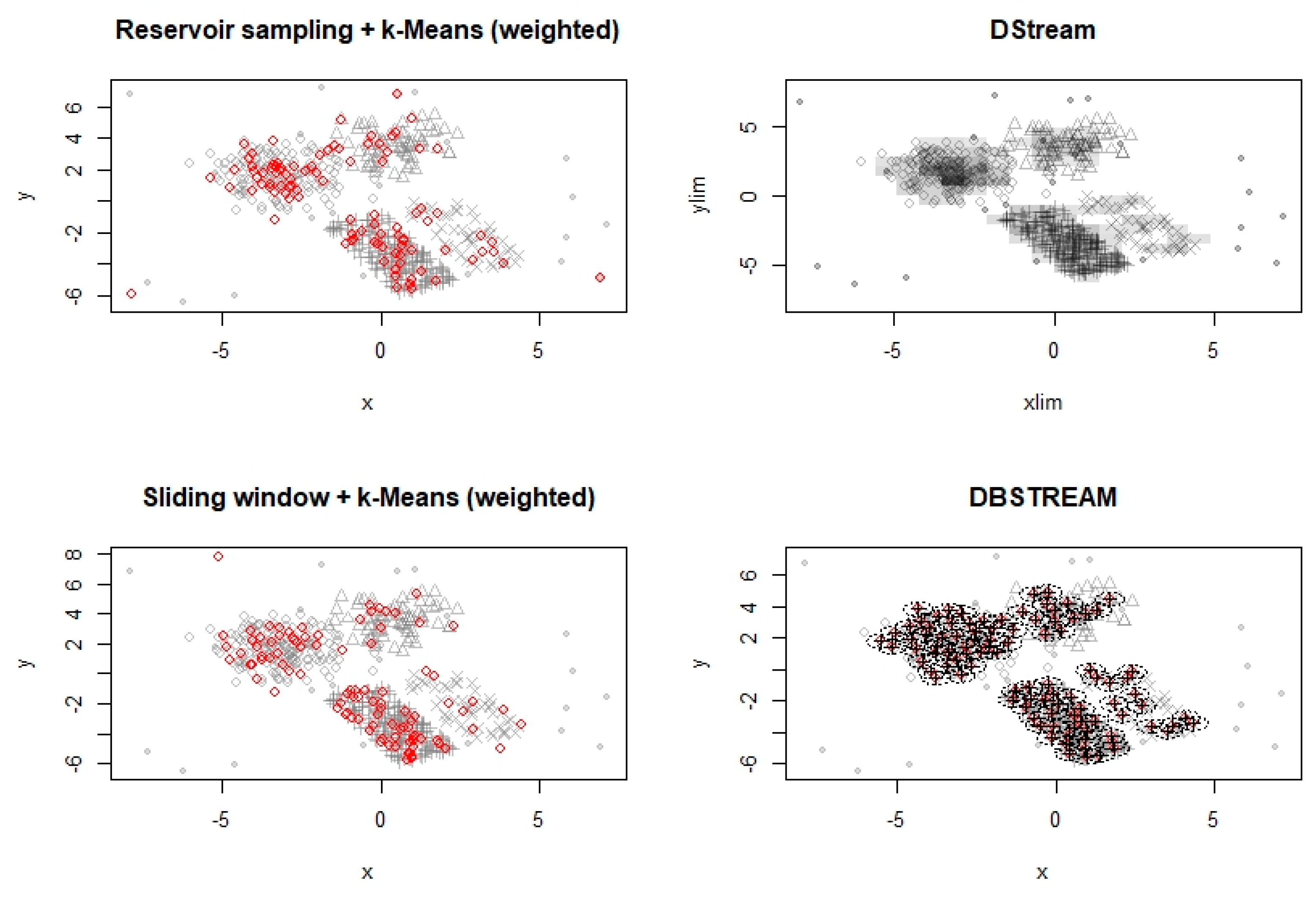
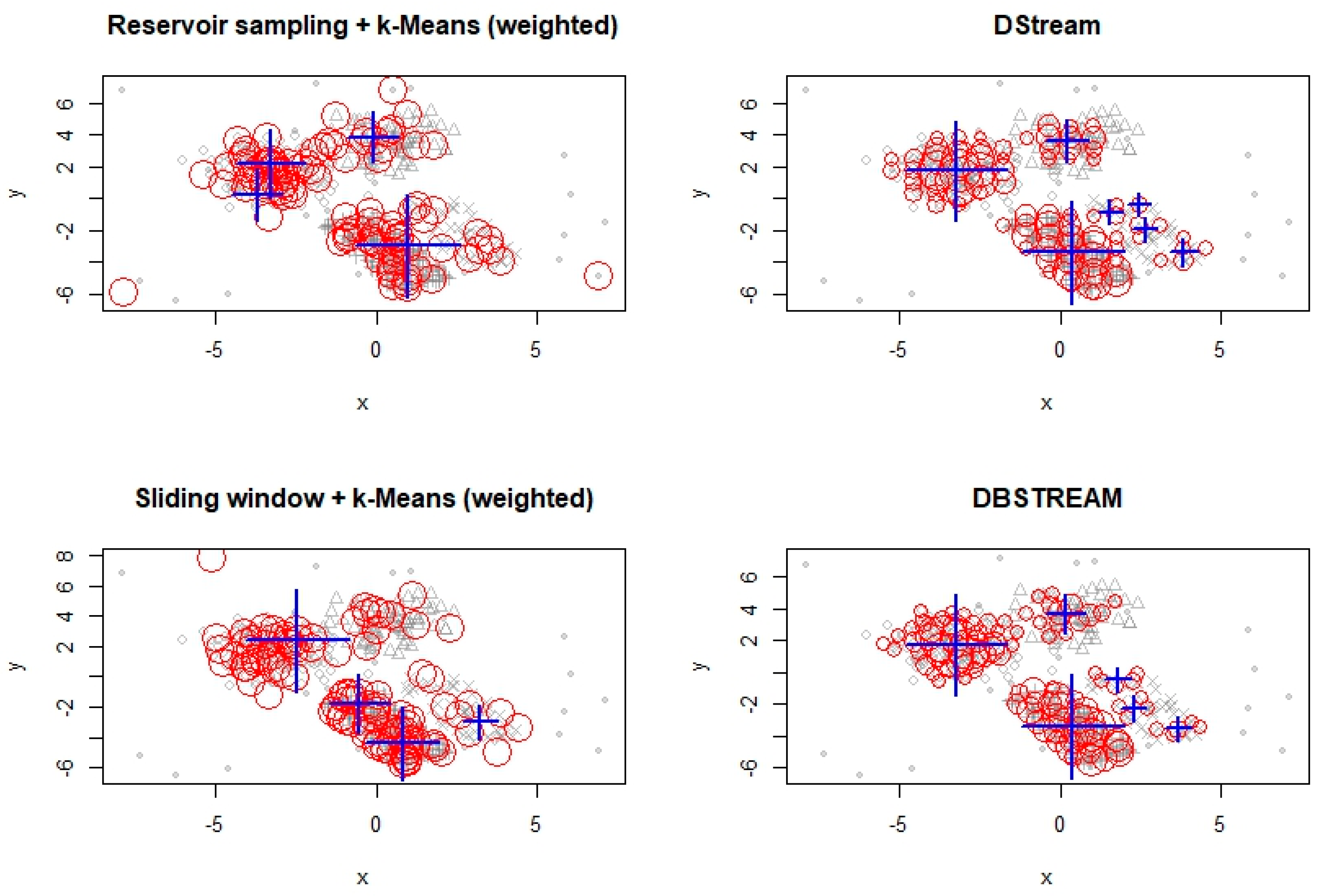
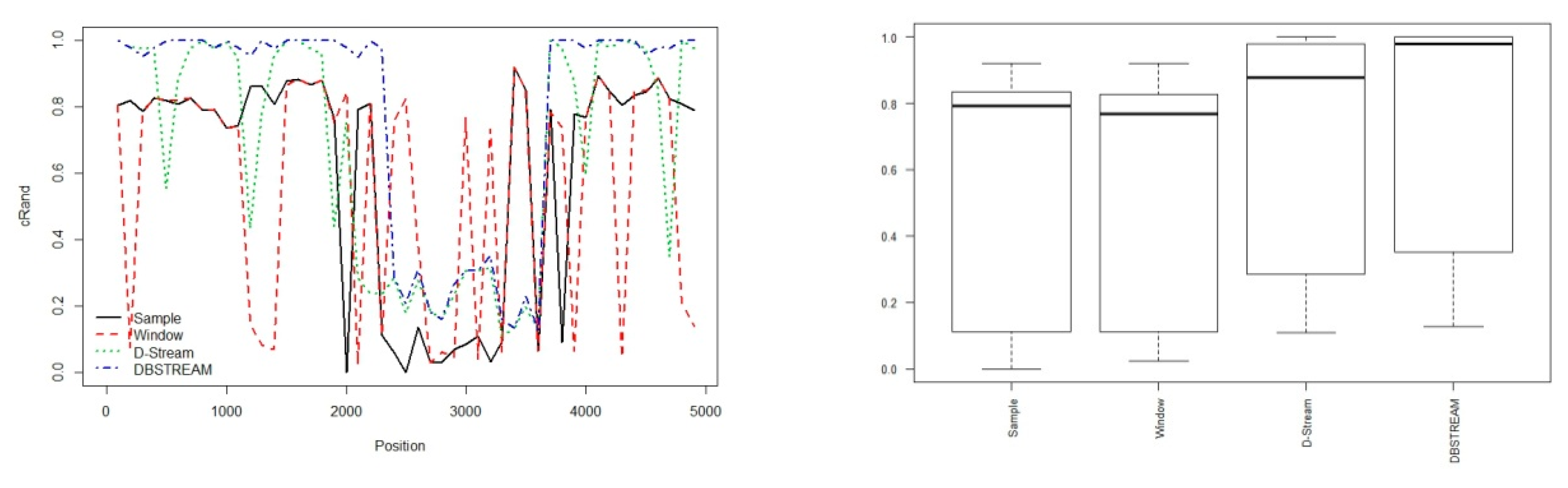
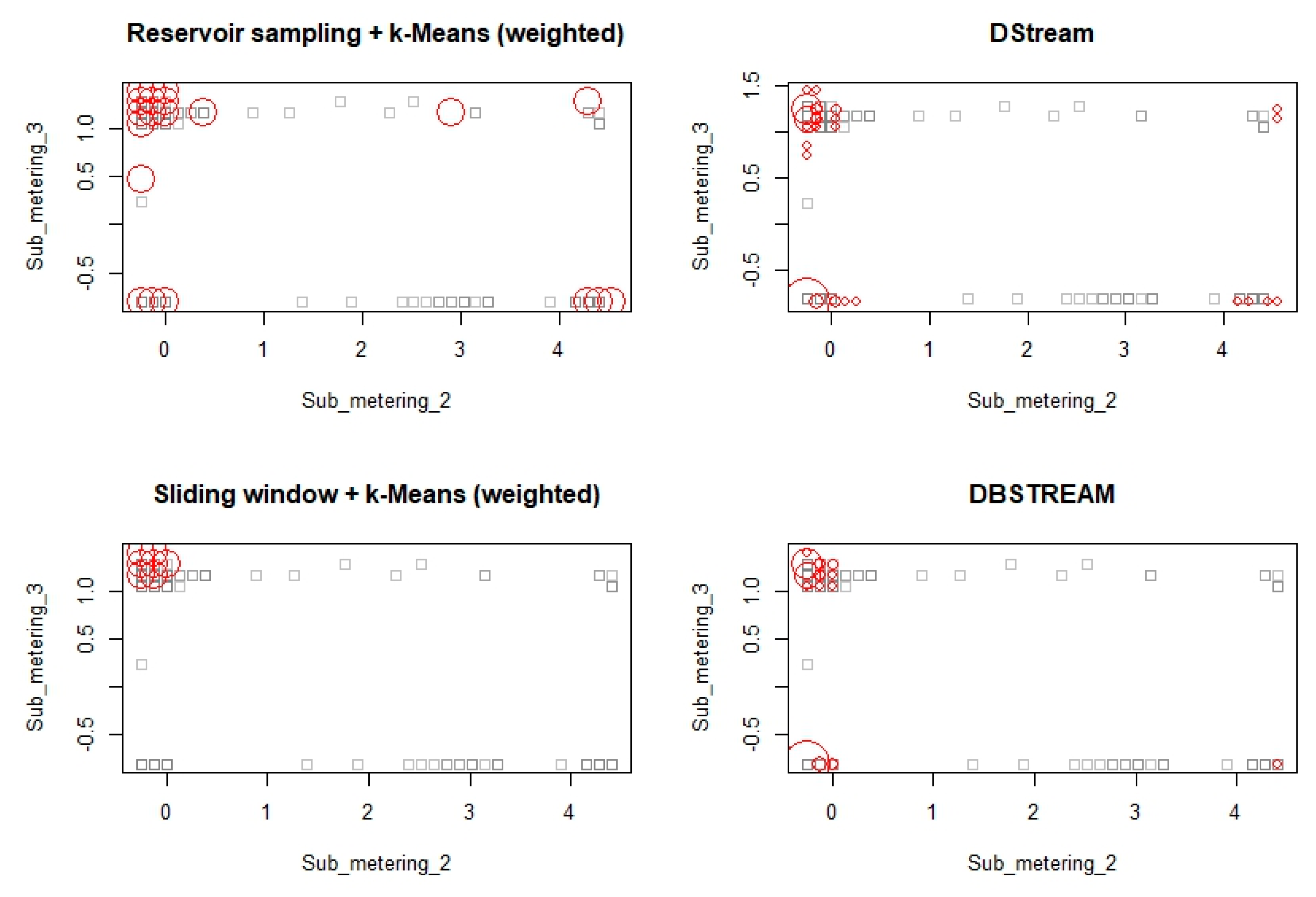
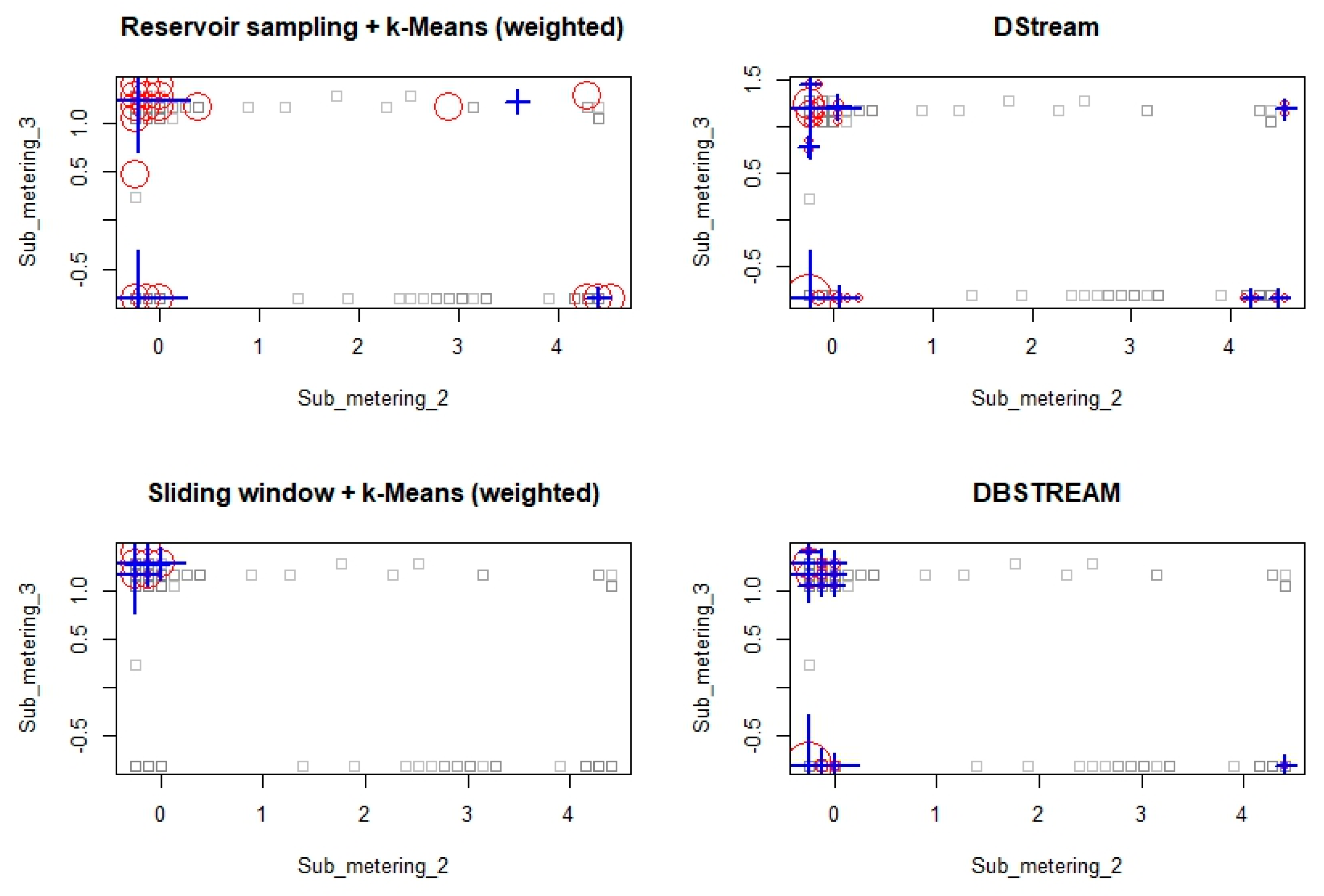
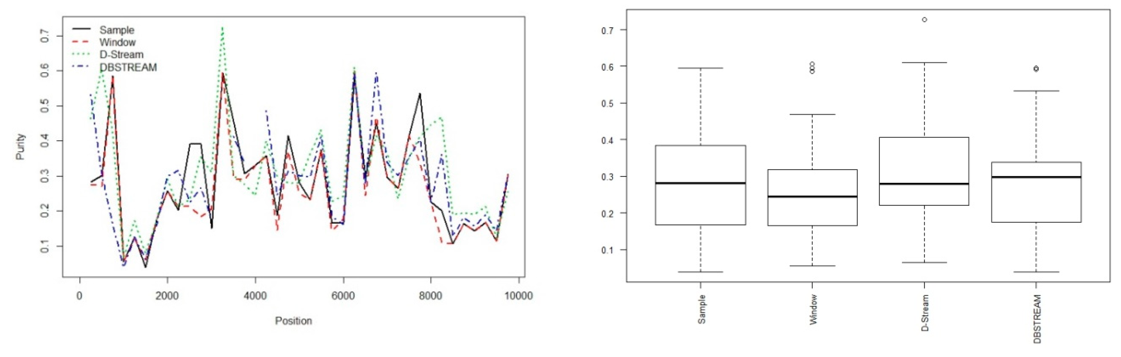
6. Experimental Results and Discussion

6.1. Experimentation with Data Streams

Some of the algorithms and techniques discussed so far are now implemented (D-Stream, DBSTREAM, Reservoir Sampling + k-means(weighted), and sliding windows +kmeans (weighted)). Comparison of these algorithms is the major purpose. A static data set is generated using stream [55,56] package in R. Around sample 1500 data points from Bars and Gaussians data stream generator of stream [55] package are extracted with 0.05% noise (1500 points are considered for experimentation purpose). First 1000 data points are used to learn clustering and next 500 points are for evaluation of these algorithms. In Figure 2 the data distribution is shown. It consists of four clusters, two Gaussians and two uniformly Filled, slightly rotated rectangular clusters. The four algorithms are initialized in stream [55] package. The algorithms are reservoir sampling re-clustered with weighted k-means, sliding window re-clustered with weighted k-means, D-Stream and DBSTREAM with their built-in re-clustering strategies. The parameters are chosen such that each shall produce approximately 100 micro-clusters.

In Figure 3, micro-cluster placement of these four algorithms is shown. Micro-clusters are shown as red circles and size is proportional to each cluster’s weights. For D-Stream values of parameters are $gridsize=0.7$ and $Cm=1.5$, here $C_m$ is parameter controlling threshold as defined in Section 3.3. For DBSTREAM radius is set as $r=0.45$. It was observed that Reservoir sampling and the sliding window select some data points as micro clusters and also include few noise points, however, D-Stream and DBSTREAM algorithms are robust to noise points and do not include these points into micro clusters. As D-Stream is grid-based, micro clusters are regularly spaces as compared to DBSTREM algorithm.

The assignment area is the area around the center of a micro-cluster in which points are considered to belong to the micro-cluster. For comparison, this appears to be interesting to visualize this for these four algorithms. Figure 4 shows the assignment area. In reservoir sampling and sliding window algorithms data points are always assigned to nearest micro-cluster, therefore it is not shown, however for DBSTREAM the assignment area for all micro-clusters is exactly the same radius, and D-Streams uses grids to show assignment area.

Micro-cluster purity index is to compare clustering quality. For each algorithm with data points which are not used for formation of the micro-clusters are deployed for such evaluation. In this case, data points are selected from 1001 onwards as first 1000 points are used for learning of clusters. Following

Table 4. Evaluation results of generated data set.

	Sample	Window	D-Stream	DBSTREAM
numMicroClusters	100.0000000	100.0000000	84.0000000	99.0000000
purity	0.9556277	0.9474273	0.9659613	0.9705846

shows the result of the same.

The results for purity for this data set are very good with reasonably well separated clusters. While comparing algorithms in terms of “purity” it is necessary to understand number of micro-clusters produced by individual algorithm, as more micro-clusters are produced, better results are obtained.

Next, macro-cluster placement is done. In case of sampling and sliding window two-stage process is created with weighted k-means method for k = 4 (the value for k is selected 4 as experimentation done with generated data with four clusters two Gaussian and two uniformly filled), D-Stream and DBSTREAM have built-in re-clustering mechanism. D-Stream joins adjacent dense grid cells to form macro-clusters and DBSTREAM joins micro-clusters reachable by overlapping assignment areas.

Figure 5 shows the macro-cluster placement. Sampling and sliding window algorithms use k-means re-clustering technique, since k = 4, they produce exactly four clusters. However, in case of D-Stream and DBSTREAM algorithms, produce the two denser clusters correctly, but split the lower density clusters into multiple pieces.

The evaluation measures at the macro-cluster level shows findings from the visual analysis of the clustering with D-Stream and DBSTREAM. These algorithms are producing the best results. It is observed that DStream and DBSTREAM do not assign some of the points which are actually not noise points will have a negative effect on the average silhouette width. Following is the result of evaluation of algorithms with respect to macro-cluster formation. The compactness of clusters in a clustering is the within-cluster sum of squares, i.e., the sum of squared distances (SSQ) between each data point and the center of its cluster. Also, in case of silhouette coefficient it was observed that, its value is very low in case of D-Stream and DBSTREAM methods. Since the number of Macro Clusters generated by D-Stream and DBSTREAM methods are seven and it is four in case of Sam1ple and Window method (which is exactly the same as data streams are generated), this shows an increase in number of clusters which results in decrease in intra-cluster average distance, and hence silhouette index is very low for D-Stream and DBSTREAM methods as compared to Sample and Window methods.

Table 5. Evaluation Results for generated data streams.

	Sample	Window	D-Stream	DBSTREAM
numMacroClusters	4.0000000	4.0000000	7.0000000	6.0000000
purity	0.8697902	0.8325503	0.8926433	0.8758753
SSQ	1199.8108788	1564.1203674	866.9658854	885.5041398
cRand	0.5811980	0.5500995	0.7820541	0.7954812
silhouette	0.4291496	0.4289753	0.3047187	0.2943902

shows results of evaluation for generated data streams.

6.2. Experimentation with Evolving Data Stream

For evolving data streams DSD_Benchmark [56] function from Stream [55] package is used. This generates two moving clusters crossing each other’s path. This generated evolving data stream is used to compare four algorithms. Initially 5000 fixed data stream points are created, and all algorithms are initialized accordingly. This time for re-clustering purpose k = 2 is selected in case of sampling and sliding window algorithms. For D-Stream and DBSTREAM, decay factor i.e., lambda is initializes to 0.01, as the cluster in the data streams move more quickly.

The four clustering algorithms are evaluated and cluster 5000 data points using the prequential evaluation method with a horizon of 250 points. Adjusted Rand Index is selected as an evaluation measure. This will generate 5000/250 = 20 evaluations for each algorithm.

Figure 6 show the Adjusted Rand Index for the four data stream clustering algorithms over the evolving data stream. It is observed that, it is not possible to separate the clusters at position 3000 when the two clusters overlap. D-Stream and DBSTREAM shows well results, where as sampling and the sliding window methods achieve only lower Adjusted Rand Index, as these algorithms cannot detect the noise and therefore tries to allocate these points to one of the cluster therefore the clusters resulting in the lower Rand Index.

6.3. Experimentation on Real-Life Data Stream

Density-based data stream clustering algorithms such as DBStream, D-Stream, and Two-stage Sampling and Sliding Window algorithms are implemented using real-life data stream available at https://archive.ics.uci.edu/ml/datasets. The data set contains consumption of electrical power at house-hold customer. It contains 207,5259 measurements gathered between December 2006 and November 2010 (47 months), with 8 attributes/labels. Attribute data type and description are shown in

Table 6. Attributes with data type.

Date	Time	global_active_power	global_reactive_power	Voltage	global_intensity	sub_metering_1	sub_metering_2	sub_metering_3
Date	Numeric	Numeric	Numeric	Numeric	Numeric	Numeric	Numeric	Numeric

and

Table 7. Description of Attributes.

Attribute Title	Description
date	Represents Date in format dd/mm/yyyy
time	Represents time in format hh:mm:ss
global_active_power	Represents household global minute averaged active power (in kilowatt).
global_reactive_power	Represents household global minute averaged reactive power (in kw).
voltage	Represents minute-averaged voltage (in volt).
global_intensity	Represents household global minute-averaged current intensity (in amp).
sub_metering_1	Represents energy sub-metering No. 1 (in watt-hour of active energy). It corresponds to the kitchen, containing mainly a dishwasher, an oven and a microwave (hot plates are not electric but gas powered).
sub_metering_2	Represents energy sub-metering No. 2 (in watt-hour of active energy). It corresponds to the laundry room, containing a washing-machine, a tumble-drier, a refrigerator and a light.
sub_metering_3	Represents energy sub-metering No. 3 (in watt-hour of active energy). It corresponds to an electric water-heater and an air-conditioner.

respectively.

In Figure 7, micro-cluster placement of these four algorithms is shown. Micro-clusters are shown as red circles and size is proportional to each cluster’s weights. For D-Stream values of parameters are $gridsize=0.1$ and $Cm=1.5$. For DBSTREAM radius is set as $r=0.36$.

It was observed that Reservoir sampling and the sliding window select some data points as micro clusters and also include few noise points, however, D-Stream and DBSTREAM algorithms are robust to noise points and do not include these points into micro clusters. As D-Stream is grid-based, micro clusters are uniformly spaces as compared to DBSTREM algorithm. Reading at sub_meter_2 and sub_meter_3 shows power consumption with respect to Global_active_power. From figure it is observed that, the micro-clusters generated by D-Stream and DBSTERAM captures almost all data points, however in case of sampling and sliding window algorithms some of the data points are missed for clustering purpose.

The assignment area is the area around the center of a micro-cluster in which points are considered to belong to the micro-cluster. Figure 8 shows the assignment area.

This visualization of the micro-cluster assignment area shows that, in case of DBSTREAM micro-clusters are exactly same as the radius. D-Stream algorithm shows grids representing assignment area as dense grids.

Figure 9 shows the macro-cluster placement. Sampling and sliding window algorithms use k-means re-clustering technique, since k = 4, they produce exactly four clusters. However, in case of D-Stream and DBSTREAM algorithms, produce the two denser clusters correctly, but split the lower density clusters into multiple pieces. D-Stream generates 9 clusters and DBSTREAM algorithm generates 11 clusters.

Considering real data stream as an evolving data stream and applying evaluation measure purity, it is observed that D-Stream and DBSTREAM shows better performance over sampling and slicing window algorithms. Also, parameters such as fading factor (lambda), gridsize, radius (r) and Cm need to be specified.

Figure 10 shows the Purity for the four data stream clustering algorithms over the evolving data stream. It is observed that, it is not possible to separate the clusters at various positions when the two clusters overlap. D-Stream and DBSTREAM shows well results, where as sampling and the sliding window methods achieve only lower Purity, as these algorithms cannot detect the noise and therefore tries to allocate these points to one of the cluster therefore the clusters resulting in the lower Purity.

It is observed that, purity, SSQ and cRand indices shows better results for D-Stream and DBSTREAM, however these indices are low for Reservoir Sampling + k-means(weighted) and Slicing window+ k-means(weighted) methods. In turn, for silhouette index it is vice versa. Therefore any single method may not able to satisfy all evaluation parameters. Also, from Figure 6 and Figure 10, it is observed that, for application’s domain specific data streams, the clustering methods leads to different evaluation result. Hence, it is necessary to select appropriate method for specific application.

7. Conclusions and Future Outlook

In this paper the problem about to identify hidden pattern and knowledge for understanding the context and identifying trends from continuous data streams are discussed. The comprehensive survey provided the study of data stream clustering methods and algorithms. The methods and algorithms are broadly categorized into five types based on methodologies adopted for implementation. This will be an ease to select appropriate algorithm for specific domain, without getting details of it. The related algorithms and methods from each category are discussed and some of them are implemented with evaluation matrix.

It is observed that, a single algorithm may not be able to satisfy all evaluation measures. Most of the density-based and density grid-based algorithms like DStream, MR-Stream, ExCC shows better performance for evolving data streams. The performance of these algorithms is measured either on synthetic data sets using statistical techniques for generating the data stream with assumed noise or on real-life data set; but there are limitations with these algorithms in order to cater evolving data streams in real-time. More research is requiring to device adaptive model for clustering evolving data streams.

As a future work, there is need to investigate the Context-based adaptive clustering methods for evolving data streams, so as to identify trends. These trends are necessary for predications and recommender system.

References

1. Aggarwal, C.C.A. Framework for Diagnosing Changes in Evolving Data Streams. In Proceedings of the ACM Sigmod, San Diego, CA, USA, 9–12 June 2003; pp. 575–586. [Google Scholar] [CrossRef]
2. Babcock, B.; Babu, S.; Datar, M.; Motwani, R.; Widom, J. Models and Issues in Data Stream Systems. In Proceedings of the ACM PODS Conference, Madison, WI, USA, 3–5 June 2002; pp. 1–16. [Google Scholar]
3. Domingos, P.; Hulten, G. Mining High-Speed Data Streams. In Proceedings of the ACM SIGKDD Conference, Boston, MA, USA, 20–23 August 2000; pp. 71–80. [Google Scholar]
4. Guha, S.; Mishra, N.; Motwani, R.; O’Callaghan, L. Clustering Data Streams. In Proceedings of the IEEE FOCS Conference, Redondo Beach, CA, USA, 12–14 November 2000; pp. 1–8. [Google Scholar]
5. Yan, S.; Lin, K.; Zheng, X.; Zhang, W.; Feng, X. An Approach for Building Efficient and Accurate Social Recommender Systems using Individual Relationship Networks. IEEE Trans. Knowl. Data Eng. 2016, 29, 2086–2099. [Google Scholar] [CrossRef]
6. Jain, A.K.; Murty, M.N.; Flynn, P.J. Data clustering: A review. ACM Comput. Surv. 1999, 31, 264–323. [Google Scholar] [CrossRef]
7. Lu, J.; Zhu, Q. Data clustering: A review. IEEE Access 2017, 5, 4991–5000. [Google Scholar] [CrossRef]
8. Hahsler, M.; Bolanos, M. Clustering Data Streams Based on Shared Density between Micro-Clusters. IEEE Trans. Knowl. Data Eng. 2016, 28, 1449–1461. [Google Scholar] [CrossRef]
9. Sun, Y.; Tang, K.; Minku, L.L.; Wang, S.; Yao, X. Online Ensemble Learning of Data Streams with Gradually Evolved Classes. IEEE Trans. Knowl. Data Eng. 2016, 28, 1532–1545. [Google Scholar] [CrossRef]
10. Mahesh, K.; Kumar, A. Rama Mohan Reddy, A fast DBSCAN clustering algorithm by accelerating neighbour searching using Groups method. Elsevier Pattern Recognit. 2016, 58, 39–48. [Google Scholar] [CrossRef]
11. Ros, F.; Guillaume, S. DENDIS: A new density-based sampling for clustering algorithm. Elsevier Expert Syst. Appl. 2016, 56, 349–359. [Google Scholar] [CrossRef]
12. Wu, X.; Zhu, X.; Wu, G.; Ding, W. Data Mining with Big Data. IEEE Trans. Knowl. Data Eng. 2014, 26, 97–107. [Google Scholar]
13. Amini, A.; YingWah, T.; Saboohi, H. On Density-Based Data Streams Clustering Algorithms: A Survey. J. Comput. Sci. Technol. 2014, 29, 116. [Google Scholar] [CrossRef]
14. Gaber, M.; Zaslavsky, A.; Krishnaswamy, S. Mining data streams: A review. ACM Sigmod Rec. 2005, 34, 18–26. [Google Scholar] [CrossRef]
15. Ikonomovska, E.; Loskovska, S.; Gjorgjevik, D. A survey of stream data mining. In Proceedings of the 8th National Conference with International Participation, Philadelphia, PA, USA, 20–23 May 2007; pp. 19–25. [Google Scholar]
16. Gaber, M.; Zaslavsky, A.; Krishnaswamy, S. Data Stream Mining, DATA Mining and Knowledge Discovery Handbook; Springer: Berlin/Heidelberg, Germany, 2010; pp. 759–787. [Google Scholar]
17. Jain, A.K.; Dubes, R.C. Algorithms for Clustering Data. In Algorithms for Clustering Data; Prentice-Hall, Inc.: Upper Saddle River, NJ, USA, 1988; ISBN 0-13-022278-X. [Google Scholar]
18. Jain, A.K. Data clustering: 50 years beyond K-means. Pattern Recognit. Lett. 2009, 31, 651–666. [Google Scholar] [CrossRef]
19. Mahdiraji, A. Clustering data stream: A survey of algorithms. Int. J. Knowl.-Based Intell. Eng. Syst. 2009, 13, 39–44. [Google Scholar] [CrossRef]
20. Amini, A.; Wah, T.; Saybani, M.A. Study of density-grid based clustering algorithms on data streams. In Proceedings of the 8th International Conference on Fuzzy Systems and Knowledge Discovery, Shanghai, China, 26–28 July 2011; pp. 1652–1656. [Google Scholar]
21. Chen, C.L.P.; Zhang, C. Data-intensive applications, challenges, techniques and technologies: A survey on big data. Inf. Sci. 2014, 275, 314–347. [Google Scholar] [CrossRef]
22. Fahad, A.; Alshatri, N.; Tari, Z.; Alamri, A.; Khalil, I.; Zomaya, A.Y.; Foufou, S.; Bouras, A.A. survey of clustering algorithms for big data: Taxonomy and empirical analysis. Trans. Emerg. Top. Comput. 2014, 2, 267–279. [Google Scholar] [CrossRef]
23. Amini, A.; Wah, T.Y. Density micro-clustering algorithms on data streams: A review. In Proceedings of the International Multiconference Data Mining and Applications, Hong Kong, China, 16–18 March 2011; pp. 410–414. [Google Scholar]
24. Amini, A.; Wah, T.Y. A comparative study of density-based clustering algorithms on data streams: Micro-clustering approaches. In Intelligent Control and Innovative Computing; Springer: Berlin/Heidelberg, Germany, 2012; pp. 275–287. [Google Scholar]
25. Aggarwal, C.C. A survey of stream clustering algorithms. In Data Clustering: Algorithms and Applications; CRC Press: Bocaton, FL, USA, 2013; pp. 457–482. [Google Scholar]
26. Hartigan, J.A.; Wong, M.A.; Means, A.K. Clustering Algorithm. J. R. Stat. Soc. Ser. C 1979, 28, 100–108. [Google Scholar] [CrossRef]
27. Han, J.; Kamber, M.; Pei, J. Cluster Analysis: Basic Concept and Methods. In Data Mining: Concept and Techniques; Morgan Kaufmann: Burlington, MA, USA, 2012; ISBN 978-0-12-381479-1. [Google Scholar]
28. Xu, R.; Wunsch, D. Survey of clustering algorithms. IEEE Trans. Neural Netw. 2005, 16, 645–678. [Google Scholar] [CrossRef] [PubMed]
29. O’Callaghan, L.; Mishra, N.; Meyerson, A.S.; Guha, R. Motwani Streaming-data algorithms for high-quality clustering. In Proceedings of the 18th International Conference on Data Engineering, Washington, DC, USA, 26 February–1 March 2002; pp. 685–694. [Google Scholar]
30. Zhang, T.; Ramakrishnan, R.; Livny, M. BIRCH: A New Data Clustering Algorithm and Its Applications. Data Min. Knowl. Discov. 1997, 1, 141–182. [Google Scholar] [CrossRef]
31. Guha, S.; Rastogi, R.; Shim, K. CURE: An efficient clustering algorithm for large databases. ACM Sigmod Rec. 1998, 27, 73–84. [Google Scholar] [CrossRef]
32. Guha, S.; Rastogi, R.; Shim, K. ROCK: A robust clustering algorithm for categorical attributes. In Proceedings of the 15th International Conference on Data Engineering (Cat. No.99CB36337), Sydney, NSW, Australia, 23–26 March 1999; pp. 512–521. [Google Scholar]
33. Karypis, G.; Han, E.; Kumar, V. Chameleon: Hierarchical clustering using dynamic modeling. Computer 1999, 32, 68–75. [Google Scholar] [CrossRef]
34. Philipp, K.; Assent, I.; Baldauf, C.; Seidl, T. The clustree: Indexing micro-clusters for anytime stream mining. Knowl. Inf. Syst. 2011, 29, 249–272. [Google Scholar]
35. Guha, S.; Meyerson, A.; Mishra, N.; Motwani, R.; O’Callaghan, L. Clustering data streams: Theory and practice. IEEE Trans. Knowl. Data Eng. 2003, 15, 515–528. [Google Scholar] [CrossRef] [Green Version]
36. Chris, F.; Raftery, A.E. MCLUST: Software for model-based cluster analysis. J. Classif. 1999, 16, 297–306. [Google Scholar]
37. Miin-Shen, Y.; Lai, C.; Lin, C. A robust EM clustering algorithm for Gaussian mixture models. Pattern Recognit. 2012, 45, 3950–3961. [Google Scholar]
38. Fisher, D.H. Knowledge acquisition via incremental conceptual clustering. Mach. Learn. 1987, 2, 139–172. [Google Scholar] [CrossRef] [Green Version]
39. Kohonen, T. The self-organizing map. Proc. IEEE 1990, 78, 1464–1480. [Google Scholar] [CrossRef]
40. Chen, Y.; Tu, L. Density-based clustering for real-time stream data. In Proceedings of the 13th ACM SIGKDD International Conference on Knowledge Discovery and Data Mining, San Jose, CA, USA, 12–15 August 2007; pp. 133–142. [Google Scholar]
41. Kranen, P.; Jansen, T.; Seidl, T.; Bifet, A.; Holmes, G.; Pfahringer, B. An Effective Evaluation Measure for Clustering on Evolving Data Streams. In Proceedings of the 17th ACM SIGKDD International Conference on Knowledge Discovery and Data Mining, San Diego, CA, USA, 21–24 August 2011; pp. 868–876. [Google Scholar]
42. Jun, W.U.; Xiong, H.; Chen, J. Adapting the Right Measures for K-means Clustering. In Proceedings of the 15th ACM SIGKDD international conference on Knowledge discovery and data mining, Paris, France, 28 June–1 July 2009; pp. 877–886. [Google Scholar]
43. Cao, F.; Ester, M.; Qian, W.; Zhou, A. Density-Based Clustering over an Evolving Data Stream with Noise. In Proceedings of the SIAM Conference on Data Mining, Bethesda, MD, USA, 20–22 April 2006; pp. 328–339. [Google Scholar]
44. Ester, M.; Kriegel, H.; Sander, J.; Xu, X. A density-based algorithm for discovering clusters in large spatial databases with noise. In Proceedings of the Second International Conference on Knowledge Discovery and Data Mining, Portland, OR, USA, 2–4 August 1996; pp. 226–231. [Google Scholar]
45. Tasoulis, D.K.; Ross, G.; Adams, N.M. Visualising the cluster structure of data streams. In Proceedings of the 7th International Conference on Intelligent Data Analysis, Oslo, Norway, 14–17 June 1999; pp. 81–92. [Google Scholar]
46. Ruiz, C.; Menasalvas, E.; Spiliopoulo, C. DenStream: Using domain knowledge on a data stream. In Proceedings of the 12th International Conference on Discovery Science, Porto, Portugal, 3–5 October 2009; pp. 287–301. [Google Scholar]
47. Liu, L.; Jing, K.; Guo, Y.; Huang, H. A three-step clustering algorithm over an evolving data stream. In Proceedings of the IEEE International Conference on Intelligent Computing and Intelligent Systems, Shanghai, China, 20–22 November 2009; pp. 160–164. [Google Scholar]
48. Ren, J.; Ma, R. Density-based data streams clustering over sliding windows. In Proceedings of the Sixth International Conference on Fuzzy Systems and Knowledge Discovery, Tianjin, China, 14–16 August 2009; pp. 248–252. [Google Scholar]
49. Lin, J.; Lin, H. A density-based clustering over evolving heterogeneous data stream. In Proceedings of the ISECS International Colloquium on Computing, Communication, Control, and Management, Sanya, China, 8–9 August 2009; pp. 275–277. [Google Scholar]
50. Isaksson, C.; Dunham, M.H.; Hahsler, M. SOStream: Self Organizing Density-Based Clustering over Data Stream. In Machine Learning and Data Mining in Pattern Recognition; MLDM 2012. Lecture Notes in Computer Science; Perner, P., Ed.; Springer: Berlin/Heidelberg, Germany, 2009; pp. 264–278. ISBN 978-3-642-31536-7. [Google Scholar]
51. Ntoutsi, I.; Zimek, A.; Palpanas, T.; Kröger, P.; Kriegel, H.P. Density-based projected clustering over high dimensional data streams. In Proceedings of the 2012 SIAM International Conference on Data Mining, Anahelm, CA, USA, April 2012; pp. 987–998. [Google Scholar]
52. Hassani, M.; Spaus, P.; Gaber, M.M.; Seidl, T. Density-based projected clustering of data streams. In Proceedings of the 6th International Conference, SUM 2012, Marburg, Germany, 17–19 September 2012; pp. 311–324. [Google Scholar]
53. Forestiero, A.; Pizzuti, C.; Spezzano, G. A single pass algorithm for clustering evolving data streams based on swarm intelligence. Data Min. Knowl. Discov. 2013, 26, 1–26. [Google Scholar] [CrossRef]
54. Garofalakis, M.; Gehrke, J.; Rastogi, R. Querying and mining data streams: You only get one look: A tutorial. In Proceedings of the 2002 ACM SIGMOD International Conference on Management of Data, Madison, WI, USA, 2–6 June 2002; p. 635. [Google Scholar]
55. Jia, C.; Tan, C.; Yong, A. A grid and density-based clustering algorithm for processing data stream. In Proceedings of the IEEE Second International Conference on Genetic and Evolutionary Computing, Wuhan, China, 25–26 September 2008; pp. 517–521. [Google Scholar]
56. Tu, L.; Chen, Y. Stream data clustering based on grid density and attraction. ACM Trans. Knowl. Discov. Data 2009, 3. [Google Scholar] [CrossRef]
57. Wan, L.; Ng, W.K.; Dang, X.H.; Yu, P.S.; Zhang, K. Density-based clustering of data streams at multiple resolutions. ACM Trans. Knowl. Discov. Data 2009, 3, 14–28. [Google Scholar] [CrossRef]
58. Ren, J.; Cai, B.; Hu, C. Clustering over data streams based on grid density and index tree. J. Converg. Inf. Technol. 2011, 6, 83–93. [Google Scholar]
59. Yang, Y.; Liu, Z.; Zhang, J.P.; Yang, J. Dynamic density-based clustering algorithm over uncertain data streams. In Proceedings of the 9th IEEE International Conference on Fuzzy Systems and Knowledge Discovery (FSKD), Chongqing, China, 29–31 May 2012; pp. 2664–2670. [Google Scholar]
60. Bhatnagar, V.; Kaur, S.; Chakravarthy, S. Clustering data streams using grid-based synopsis. Knowl. Inf. Syst. 2014, 41, 127–152. [Google Scholar] [CrossRef]
61. Hahsler, M.; Bolanos, M.; Forrest, J. Introduction to stream: An Extensible Framework for Data Stream Clustering Research with R. J. Stat. Softw. 2017, 76, 1–50. [Google Scholar] [CrossRef]
62. Pandove, D.; Goel, S.; Rani, R. Systematic Review of Clustering High-Dimensional and Large Datasets. ACM Trans. Knowl. Discov. Data 2018, 12, 4–68. [Google Scholar] [CrossRef]
63. Aggarwal, C.C.; Wang, J.Y.; Yu, P.S. A Framework for Projected Clustering of High Dimensional Data Streams. In Proceedings of the Thirtieth International Conference on Very Large Data Bases, Toronto, ON, Canada, 31 August–3 September 2004. [Google Scholar]
64. Zhou, A.; Cao, F.; Qian, W.; Jin, C. Tracking clusters in evolving data streams over sliding windows. Knowl. Inf. Syst. 2008, 15, 181–214. [Google Scholar] [CrossRef]
65. Liadan, O.; Mishra, N.; Meyerson, A.; Guha, S.; Motwani, R. Streaming-data algorithms for high-quality clustering. In Proceedings of the 18th International Conference on Data Engineering, Washington, DC, USA, 26 February–1 March 2002. [Google Scholar]
66. Dempster, P.A.; Laird, N.M.; Rubin, D.B. Maximum likelihood from incomplete data via the EM algorithm. J. R. Stat. Soc. Ser. B 1977, 39, 1–38. [Google Scholar]
67. Dang, X.H.; Lee, V.; Ng, W.K.; Ciptadi, A.; Ong, K.L. An EM-based algorithm for clustering data streams in sliding windows. In International Conference on Database Systems for Advanced Applications; Springer: Berlin/Heidelberg, Germany, 2009. [Google Scholar]
68. Damminda, A.; Halgamuge, S.K.; Srinivasan, B. Dynamic self-organizing maps with controlled growth for knowledge discovery. IEEE Trans. Neural Netw. 2000, 11, 601–614. [Google Scholar] [Green Version]
69. Toby, S.; Alahakoon, D. Growing self-organizing map for online continuous clustering. In Foundations of Computational Intelligence Volume 4; Springer: Berlin/Heidelberg, Germany, 2009; pp. 49–83. [Google Scholar]
70. Chow, T.W.S.; Wu, S. An online cellular probabilistic self-organizing map for static and dynamic data sets. IEEE Trans. Circuits Syst. Regul. Pap. 2004, 51, 732–747. [Google Scholar] [CrossRef]
Figure 1. Categorization of Clustering Algorithms.
Bdcc 02 00032 g001
Figure 2. Bars and Gaussians Data Set.
Bdcc 02 00032 g002
Figure 3. Micro-cluster placement for different data stream clustering algorithms.
Bdcc 02 00032 g003
Figure 4. Micro-cluster assignment areas for different data stream clustering algorithms.
Bdcc 02 00032 g004
Figure 5. Macro-cluster placement for different data stream clustering algorithms.
Bdcc 02 00032 g005
Figure 6. Evaluation of data stream clustering of an evolving stream.
Bdcc 02 00032 g006
Figure 7. Micro-cluster placement for different algorithms. Reading of sub_meter_1 and sub_meter_2 are selected for formation of clusters (using real data stream).
Bdcc 02 00032 g007
Figure 8. micro-cluster assignment area for different data stream clustering algorithms (using real data stream).
Bdcc 02 00032 g008
Figure 9. Macro-cluster placement for different data stream clustering algorithms (using real data stream).
Bdcc 02 00032 g009
Figure 10. Evaluation of data stream clustering of an evolving stream (using real data stream).
Bdcc 02 00032 g010