Isolating Graph Topology from Model Architecture in GNN-Based Fraud Detection: An Empirical Framework

Abstract

Graph topology and model architecture are routinely co-designed in GNN-based fraud detection, making it impossible to attribute performance gains to either component. We address this by fixing the training loop, features, and evaluation protocol while independently varying the graph construction strategy and GNN architecture. Three strategies are evaluated: multi-relation temporal, hybrid structural similarity, and intra-group, each evaluated across three GNN architectures (GATv2, GCN, and GraphSAGE). A feature-identical MLP with no graph structure serves as an empirical anchor. On the Sparkov dataset, all three GNN strategies exceed the MLP by 5.0–9.7 F1 points, confirming that topology contributes genuine discriminative value when per-cardholder histories are dense. On the IBM dataset, the intra-group strategy collapses 6.9 F1 points below the MLP, a consequence of near-empty neighbourhoods (mean degree 1.1) following down-sampling, while multi-relation retains ranking advantages in AUC (Area Under the Curve; 0.985) and Average Precision (0.908) despite marginal F1 parity. Across both datasets, multi-relation temporal construction is the highest-performing strategy, achieving F1 0.908 and AUC 0.994 on Sparkov and F1 0.831 on IBM, though this ranking is not entirely architecture-independent: GraphSAGE narrowly inverts the multi-relation/intra-group order on Sparkov. These results suggest that graph construction quality, rather than mere graph presence, matters more for GNN performance than connectivity alone under the conditions evaluated here.

1. Introduction

Credit card fraud imposes measurable economic harm at scale, yet the gap between detection research and deployable, interpretable systems continues to widen. Rule-based methods and classical machine learning classifiers have been widely deployed, but both struggle to generalise as fraud tactics evolve [1]. Recent advances in deep learning and graph-based modelling have improved detection performance [2,3], yet existing systems couple graph construction with model architecture in end-to-end designs, making it impossible to attribute performance gains to either component independently; prior ablations vary graph structure within coupled systems where model and graph are co-designed, preventing attribution [4,5]. A persistent open question is whether performance gains in such systems originate from the graph topology or from the neural operator applied to it: because graph construction and model architecture are always co-optimised, the two contributions cannot be disentangled. To the best of our knowledge, this study provides a controlled empirical comparison of graph construction strategies under a common training pipeline and evaluation protocol, enabling a systematic investigation of their impact across multiple GNN architectures, rather than proposing a new architecture or learning method.

This paper addresses that gap by proposing a unified modular framework that treats graph construction strategy as the primary experimental variable, holding architecture and all other pipeline components fixed. Three construction strategies (multi-relation temporal, hybrid structural similarity, and intra-group) are implemented as pluggable, configuration-only components evaluated under three GNN architectures (GATv2, GCN, and GraphSAGE), with all other pipeline components (training loop, optimiser, loss function, cross-validation protocol, and leakage safeguards) held strictly fixed across all runs. A feature-identical MLP with no graph structure serves as an empirical anchor. Running each graph strategy under multiple architectures additionally allows us to test whether topology performance rankings are an artefact of one operator or a reproducible property of graph construction quality itself.

Our contributions are four-fold. First, we present a reusable experimental framework that keeps architecture-independent components fixed while varying the graph construction strategy and, independently, the GNN architecture. This controlled design enables the effects of the graph construction strategy and message-passing architecture to be systematically evaluated while keeping the remaining components of the learning pipeline consistent. Second, we show that multi-relation temporal graph construction generally achieves the strongest overall performance across the evaluated datasets and GNN architectures, although the relative ranking of graph construction strategies exhibits some architecture-dependent variation. Third, we show that graph construction quality appears to have a greater influence on GNN performance than graph density alone under the evaluated experimental conditions. Specifically, FAISS-based (Facebook AI Similarity Search) similarity edges provide limited benefit when strong relational information is already available, whereas intra-group strategies approach MLP-level performance when per-cardholder transaction histories are sparse. This behaviour is consistently observed across GATv2 (Graph Attention Network v2), GCN (Graph Convolutional Network), and GraphSAGE (Graph Sample and Aggregate). Fourth, we present a leakage-safe experimental framework that combines group-stratified data splitting, temporal ordering, and training-only feature normalisation to minimise information leakage throughout model development and evaluation, thereby improving the reliability and reproducibility of experimental comparisons.

The rest of this paper is organised as follows. Section 2 reviews related work on graph-based fraud detection. Section 3 describes the proposed framework and graph construction strategies. Section 4 details the experimental setup. Section 5 presents the results including graph topology analysis, confusion matrices, and comparison with a feature-identical MLP (multi-layer perceptron) baseline. Section 6 compares the proposed method against published results on the same datasets. Section 7 discusses strategy performance and density effects, score calibration, and controlled ablation insights. Section 8 discusses the limitations.

2. Related Work

GNN-based fraud detection has advanced rapidly, yet every published system couples graph construction and model architecture within a single end-to-end design. This coupling is not merely incidental: when both components are optimised together, any observed performance gain cannot be attributed to topology alone, because the architecture may have been specifically tuned to exploit the chosen graph structure. The dominant paradigm links transactions across cardholders through shared attributes such as merchants, device identifiers, or geographic proximity. Ref. [6] builds a weighted multi-relational graph with temporal attention on GraphSAGE, achieving improved F1 on a real-world dataset, but the graph and attention mechanism are jointly designed, precluding topology attribution. Ref. [7] uses an Edge-GCN over cardholder–merchant bipartite graphs, achieving F1 = 0.71 and AUC = 0.87 on IBM, with the bipartite structure inseparable from the edge convolution operator. Ref. [8] reports F1 = 0.854 with heterogeneous GAT on a proprietary simulated dataset distinct from Sparkov and IBM, making direct numerical comparison with our results inappropriate. Attention-based variants [9,10] extend this coupling pattern to healthcare and cryptocurrency fraud, confirming it is a systemic limitation of the field rather than a property of any individual method.

A complementary design restricts graph construction to within individual cardholder histories, avoiding the context dilution that arises when edges span behaviourally unrelated accounts. Where the cross-cardholder paradigm [2,7,8] prioritises ring detection and shared attribute connectivity, the intra-group design preserves per-account anomaly signals and enables richer temporal modelling within each cardholder sequence. In our own prior work [11], we evaluated a multi-edge intra-group construction in isolation combining temporal, similarity, and merchant sub-relation edges within a single cardholder’s transaction history and found that performance depends critically on per-cardholder transaction density: F1 = 0.909 on the dense Sparkov dataset versus F1 = 0.763 on the sparse IBM dataset. However, that study evaluated intra-group construction on its own, without a controlled comparison against cross-cardholder or hybrid topologies under an identical architecture, leaving open whether the observed density sensitivity is a property of intra-group construction specifically or a general property of sparse transaction graphs. The present framework directly addresses this by evaluating intra-group construction alongside two alternative topologies under one fixed architecture and protocol, allowing the density effect to be compared alongside the choice of topology, rather than fully separated from it.

Evaluation rigour is a further concern across existing work. Ref. [12] integrates R-GCN (Relational Graph Convolutional Network) into a fraud detection pipeline reporting 99.88% accuracy on IBM, a metric that is uninformative at a 0.12% fraud rate, where a majority classifier achieves identical accuracy without detecting a single fraud case. Ref. [13] applies heuristic graph thresholds on Sparkov, achieving F1 = 0.773 while relying entirely on hand-crafted rules rather than learned representations, demonstrating that graph structure provides a signal but stopping short of a learned, reproducible model. Beyond metric choice, attribution is further confounded by experimental design: ablations that vary graph structure [2,7,8] are always conducted within the same coupled system, so the architecture was co-designed with the graph being ablated; and GNN-versus-MLP comparisons [12] frequently differ in feature sets, class imbalance handling, or threshold strategy across conditions, making it impossible to isolate topology as the source of any difference. No prior work simultaneously enforces group-stratified splitting, temporal ordering, and training-only feature normalisation, the three safeguards needed to prevent the most common leakage pathways. The present framework addresses these concerns by fixing every experimental variable except graph topology, reporting threshold-free ranking metrics alongside F1, and enforcing all three leakage safeguards simultaneously.

3. Materials and Methods

3.1. Problem Formulation

We formulate credit card fraud detection as a node-level binary classification problem on a homogeneous graph. Each transaction is modelled as a node v_i with feature vector x_i consisting of categorical embeddings and scaled numerical features. The label y_i ∈ {0, 1} indicates whether the transaction is fraudulent. The graph G = (V, E) is constructed by a pluggable strategy function φ: V × V → {0, 1} that determines, for each pair of nodes, whether an edge exists between them, based on relational, temporal, or feature similarity criteria; applying φ across all node pairs in V yields the edge set E. Different strategy functions φ induce structurally distinct graphs over the same node set V, ranging from globally connected graphs that link transactions across cardholders through shared attributes, to fully partitioned graphs {G₁, G₂, …, G_k} where edges are scoped within individual cardholder groups and K is the number of unique cardholders. The central experimental variable in this framework is φ; all other components, node features, training procedure, and evaluation protocol are held constant across strategies within each architecture run; architecture is varied separately in Section 5.4.

3.2. Framework Architecture

The proposed framework follows a modular pipeline architecture consisting of five stages: (1) data loading and preprocessing, (2) train-fitted feature engineering with no data leakage, (3) pluggable graph construction, (4) GNN model training (GATv2, GCN, or GraphSAGE) with early stopping, and (5) ensemble evaluation with threshold tuning. The graph construction stage accepts a strategy parameter that selects among three implementations while all other stages remain identical, ensuring that observed performance differences are attributable solely to graph topology.

3.3. Graph Construction Strategies

We implement three graph construction strategies, each encoding a distinct hypothesis about the relational structure most informative for fraud detection.

• Strategy 1: Multi-Relation Temporal. This strategy constructs edges by grouping transactions along multiple relational columns, such as card identifier, user, merchant name, and merchant category code, and connecting temporally adjacent transactions within each group. For each relational column, transactions sharing the same attribute value are sorted by timestamp and each transaction is linked to its k_r = 3 nearest temporal neighbours within the group. 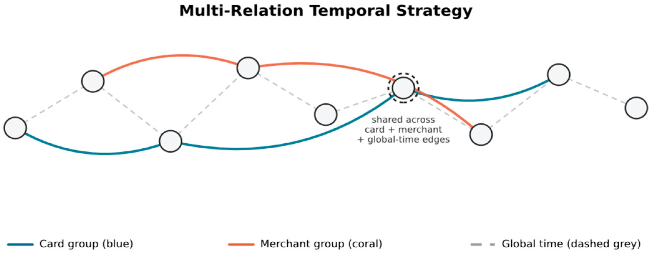k_r = 3 was selected to capture short-range sequential dependencies while limiting per-node degree growth across four relational columns. All temporal edges, in this and the other two strategies, are treated as bidirectional and include self-loops, consistent with the homogeneous, undirected message-passing formulation used throughout. Additionally, global temporal edges connect consecutive transactions across the entire dataset regardless of group membership. All edge sources are merged into a single deduplicated homogeneous set, giving the GATv2 attention mechanism access to neighbours from diverse relational contexts simultaneously. As Figure 1 illustrates, the same transaction can appear as a node in multiple relational passes, for example, a single transaction shares an edge with its temporally adjacent card transaction, its temporally adjacent merchant transaction, and its globally adjacent transaction, all within the same merged graph.

• Strategy 2: Hybrid Structural Similarity. This strategy inherits all multi-relation temporal edges and augments them with feature similarity edges computed via FAISS approximate nearest neighbour search [14]. Transaction features (scaled numerical and encoded categorical) are L2-normalised and indexed using an HNSW (Hierarchical Navigable Small World) structure for inner product similarity. The k_s nearest transactions in feature space become additional bidirectional edges, where k_s is set per dataset based on graph density calibration: k_s = 6 on Sparkov and k_s = 4 on IBM. The lower value on IBM reflects the dataset’s larger node count in the Fold 1 training graph (211,649 vs. 33,815), where a higher k_s would produce prohibitively dense graphs and disproportionately increase the ratio of similarity edges to relational edges, further diluting the structural signal. 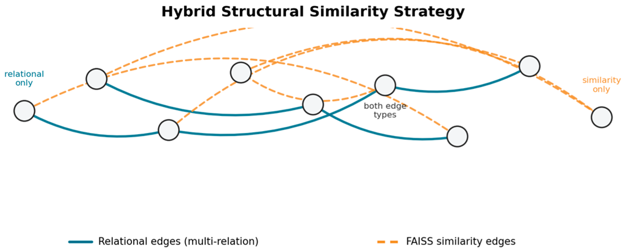Both values were selected to approximately match the average degree of the relational edges on each dataset (10.4 on Sparkov, 4.3 on IBM), ensuring that similarity edges augment rather than overwhelm the domain-driven structure; sensitivity to alternative k_s values is acknowledged as a direction for future work. To prevent leakage, the FAISS index is built exclusively from training set node features; test nodes query this index inductively to retrieve their nearest neighbours from the training set, ensuring no test set information influences edge construction. This combines domain-driven structural knowledge with data-driven behavioural similarity in a single homogeneous graph, directly testing whether feature space proximity provides complementary signal beyond relational structure. As Figure 2 illustrates, not every transaction necessarily receives both edge types in a given instance; a node may have only a relational edge, only a similarity edge, or both but every node is eligible for either, since the two edge sets are computed independently of one another over the same set of transactions within a given split (i.e., all multi-relation and FAISS similarity edges for a training fold graph are built from that fold’s training transactions only, per the train-only FAISS index described above) before being merged.

• Strategy 3: Intra-Group. This strategy scopes all edge construction within a single group key, such as the cardholder identifier, serving as a controlled baseline within the unified framework, and follows the multi-edge construction introduced in our prior work [11] Within each group, three complementary edge types are constructed: (a) temporal sequential chains linking each transaction to its k_t = 3 previous transactions, matching the temporal lookback depth used in Strategy 1; (b) cosine similarity edges connecting the top-k^c = 5 most similar transactions above a threshold τ = 0.5, with k^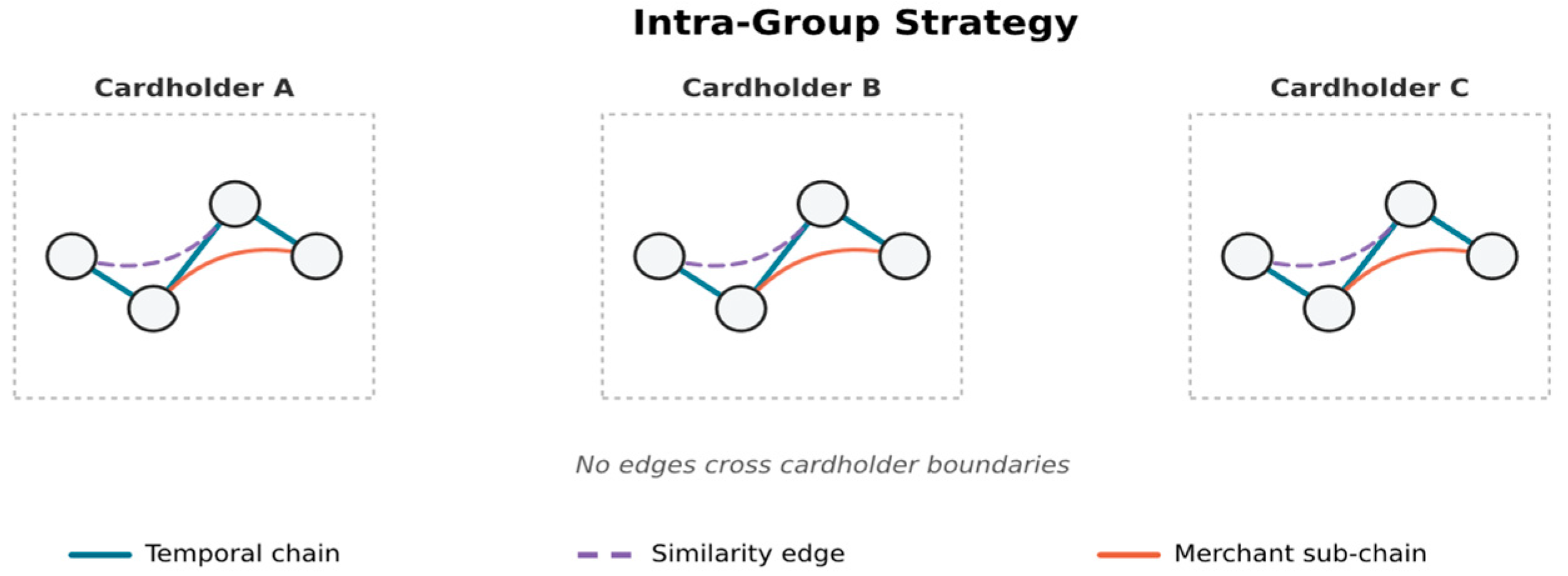c and τ selected to retain a small set of highly relevant neighbours while excluding weak similarity matches; and (c) merchant sub-relation chains linking consecutive transactions at the same merchant. No edges cross cardholder boundaries, making each cardholder a self-contained subgraph. Unlike [11], which evaluates this construction in isolation, here, it is compared directly against Strategies 1 and 2 under an identical architecture and protocol. Figure 3 illustrates this approach.

3.4. GATv2 Model Architecture

We use a two-layer GATv2 [15], which computes dynamic attention coefficients that depend on both source and target node features, allowing the attention function to assign different neighbour importance depending on the query node. This expressiveness is particularly relevant for our formulation, where temporal neighbours, similarity neighbours, and merchant chain neighbours coexist within the same graph and require different attention weights depending on their relevance to fraud detection.

Each layer applies GATv2Conv with 32 hidden units and 2 attention heads on IBM (64 hidden units and 4 heads on Sparkov), producing a 64-dimensional (IBM) or 256-dimensional (Sparkov) node representation. LayerNorm and LeakyReLU activation are applied between layers, followed by dropout (p = 0.30). A two-layer MLP classifier (Linear hidden → 128, LeakyReLU, Dropout, Linear 128 → 1) maps node embeddings to a single logit per transaction. Categorical features are encoded via learned embedding tables (dimension 8 per high-cardinality column and dimension 4 per low-cardinality column on IBM; dimension 8 per column on Sparkov) and concatenated with StandardScaler-normalised numerical features. The model is trained using BCEWithLogitsLoss with an automatically computed positive class weight.

For the GCN and GraphSAGE variants reported in Section 5.4, the GATv2Conv layers are replaced with two-layer GCNConv [16] and SAGEConv [17] (mean aggregation) layers respectively, with the hidden dimension set to match GATv2’s effective output size on each dataset (64 on IBM; 256 on Sparkov). All other architectural components LayerNorm, LeakyReLU activation between layers, the two-layer classifier head (Linear → 128, LeakyReLU, Dropout, Linear → 1), embedding tables, and dropout (p = 0.30)—are held identical across all three GNN architectures on a given dataset.

3.5. MLP Baseline

To provide a non-graph empirical anchor, we implement a feature-identical multi-layer perceptron (MLP) baseline that receives the same per-transaction inputs as the GATv2 model categorical features encoded via the same learned embedding tables (dimension 8 per high-cardinality column and dimension 4 per low-cardinality column on IBM; dimension 8 per column on Sparkov, matching the GNN encoders described in Section 3.4) and StandardScaler-normalised numerical features but performs no message passing and has no access to graph structure; each transaction is classified independently of its neighbours. The MLP is a three-layer feedforward network (Linear input → 256, LeakyReLU, Dropout (p = 0.30), Linear 256 → 128, LeakyReLU, Dropout, Linear 128 → 1), so that differences in performance reflect the presence or absence of neighbourhood aggregation rather than a difference in model capacity. The MLP is trained under the identical protocol described in Section 3, the same optimiser, learning rate schedule, loss function with automatically computed positive class weight, gradient clipping, early stopping criterion, group-stratified 5-fold cross-validation, pooled validation threshold tuning, and 5-fold ensemble averaging at test time, so that the presence or absence of neighbourhood aggregation remains the sole variable distinguishing the MLP from any given GNN strategy run under the same architecture. The MLP baseline is reported alongside all three graph construction strategies in Section 5.2 and Section 5.3, and against the GCN and GraphSAGE results in Section 5.4.

3.6. Training and Evaluation Protocol

Data splitting: Each dataset is partitioned into a training set (80%) and a held-out test set (20%) using a group-aware hold-out split based on user identity, ensuring that all transactions from a given user appear exclusively in either the training or test set, but never both. Within the training set, group-stratified 5-fold cross-validation generates train/validation splits. The held-out test set remains completely unseen throughout training, validation, and threshold tuning.

Training: Models are trained with AdamW (lr = 1 × 10⁻³, weight_decay = 1 × 10⁻⁴) and CosineAnnealingWarmRestarts (T₀ = 20, T_m = 2, η_min = 1 × 10⁻⁵). Gradient clipping is applied at norm 1.0. Early stopping monitors validation Average Precision every 5 epochs with patience of 12 checks.

Threshold selection: After training, the classification threshold is tuned to maximise the F1 score on the pooled validation predictions across all 5 folds. The resulting thresholds differ meaningfully across strategies and datasets, reflecting each strategy’s score distribution.

Test evaluation: Predicted probabilities from all 5-fold models are averaged (ensemble) and evaluated on the held-out test set using the pooled validation threshold. All reported performance metrics are from this held-out test set only.

Algorithm 1: Evaluation pipeline. The following steps clarify the exact order of operations and make explicit which components see which data at each stage: (1) Split the full dataset 80/20 by group key (cardholder/user identity) via group-aware hold-out; no group appears in both the development and held-out test sets. (2) Within the 80% development set, generate 5 group-stratified train/validation folds. (3) For each fold, fit all feature engineering statistics (StandardScaler, categorical factor maps, user/cardholder aggregate features, and, for the hybrid strategy, the FAISS index) on that fold’s training partition only. (4) Construct the graph for that fold’s training and validation transactions using the selected strategy, applying the fold’s fitted statistics to validation nodes without refitting. (5) Train the model with early stopping on validation Average Precision. (6) Tune the classification threshold to maximise F1 on pooled validation predictions across all 5 folds. (7) At test time, apply each fold’s fitted (training-only) statistics and the same graph construction rule to the held-out test transactions, average the 5-fold models’ predictions (ensemble), and apply the pooled threshold. This pipeline is mixed inductively/transductively: node features and edge construction rules generalise inductively to unseen test transactions (no test set statistics are used in fitting), but because graph edges may still connect transactions within the same split (e.g., two test transactions from the same cardholder), message passing at test time can draw on other test set nodes’ raw features, which is standard practice for graph-based fraud detection but distinct from a purely inductive, single-node-at-a-time inference setting.

4. Experimental Setup

4.1. Datasets

The Sparkov dataset [18] contains 1.85 M transactions at an approximately 0.1% fraud rate. Non-fraud transactions are randomly down-sampled prior to the group-aware train/test split to achieve an 18.4% fraud rate, after which 52,394 transactions remain with 27 engineered features, including cyclic hour encodings, customer–merchant distance, amount relative to cardholder average, and inter-transaction time differences. All group-level aggregate features including amount relative to cardholder average are computed on training transactions only and applied to validation and test sets using training-derived statistics, preventing feature leakage.

The IBM dataset [19] contains 24.4 M synthetic transactions at a 0.09% fraud rate. Prior to the group-aware split, all 29,757 fraud cases are retained, and non-fraud transactions are randomly down-sampled to a 1:10 non-fraud ratio, producing 327,327 transactions at a 9.09% fraud rate with 23 features, including user-spending normalisation fitted on training data only to prevent leakage. For test set users with no training set transaction history, the user-average feature falls back to the training set global average rather than being left undefined, ensuring every test node receives a valid feature vector without using any test set statistics. The 1:10 ratio was chosen to preserve all minority-class examples while remaining computationally tractable for graph construction; practitioners deploying this framework at natural fraud rates (0.1–1%) will encounter different graph density conditions, and the results on Sparkov (18.4% fraud after down-sampling) should be interpreted accordingly. The IBM dataset was originally released as a synthetic anti-money laundering benchmark [19]; we repurpose its binary transaction-level label as a fraud detection target consistent with its use in prior GNN fraud detection work on this dataset [7,12]. The results on IBM should therefore be read as evidence for the detection of illicit transaction patterns broadly, rather than as narrowly scoped to card-present or card-not-present fraud as represented by Sparkov.

4.2. Evaluation Metrics

Given the class imbalance (18.42% fraud in Sparkov, 9.09% in IBM), standard accuracy is uninformative; we report F1, precision, recall, AUC-ROC, and Average Precision uniformly across all strategies, with thresholds tuned to maximise F1 on the pooled 5-fold validation predictions and test evaluation using ensemble averaging.

5. Results

5.1. Graph Topology

Table 1. Graph topology statistics by strategy and dataset (Fold 1 training set).

Dataset	Strategy	Nodes	Edges	Min Deg	Max Deg	Avg Deg
Sparkov	Multi-rel	33,815	352,233	6	12	10.4
Sparkov	Hybrid	33,815	583,875	11	28	17.3
Sparkov	Intra-grp	33,815	407,381	6	18	12.0
IBM	Multi-rel	211,649	916,245	1	9	4.3
IBM	Hybrid	211,649	2,127,697	5	59	10.1
IBM	Intra-grp	211,649	223,583	1	20	1.1

Note: because the hybrid strategy’s FAISS HNSW index performs approximate nearest-neighbour search, its exact edge count and degree statistics vary marginally (<0.1%) between otherwise-identical runs; the multi-relation and intra-group edge sets are constructed deterministically and reproduce exactly across runs.

summarises the graph properties produced by each strategy from the Fold 1 training graphs, demonstrating substantial structural differences between strategies operating on identical underlying data. On Sparkov, multi-relation produces moderately connected graphs (avg. degree 10.4, range 6–12), reflecting consistent temporal chains across four relational columns. Hybrid produces the densest graphs (avg. degree 17.3, range 11–28), adding FAISS similarity edges on top of relational structure. Intra-group produces intermediate density (avg. degree 12.0, range 6–18) with tighter bounds due to the within-cardholder scoping.

On IBM, the contrast is more striking. Multi-relation produces sparse graphs (avg. degree 4.3, range 1–9) due to the limited temporal resolution of the dataset (hour: minute only) and absence of geolocation. Hybrid partially compensates with FAISS similarity edges (avg. degree 10.1, range 5–52), but intra-group collapses to near-minimal connectivity (avg. degree 1.1, median 1.0), meaning most nodes are connected only through self-loops. This is a direct consequence of down-sampling: retaining all 29,757 fraud cases but only a 1:10 non-fraud ratio reduces most cardholders to one or two transactions, making meaningful within-cardholder graph construction impossible.

5.2. Sparkov Dataset Results

Five-fold cross-validation on Sparkov confirms stable generalisation across all strategies (

Table 2. Cross-validation (pooled validation fold) F1 and AUC by dataset and strategy.

Dataset	Strategy	Val F1	Val AUC
Sparkov	Multi-relation	0.922	0.992
Sparkov	Hybrid	0.865	0.976
Sparkov	Intra-group	0.915	0.988
Sparkov	MLP Baseline	0.816	0.966
IBM	Multi-relation	0.805	0.978
IBM	Hybrid	0.797	0.976
IBM	Intra-group	0.743	0.953
IBM	MLP Baseline	0.821	0.969

): multi-relation achieves the strongest validation F1 (0.922), intra-group is comparable (0.915), and hybrid shows a larger gap (0.865), indicating that FAISS similarity edges provide less transferable signal.

Multi-relation and intra-group are nearly indistinguishable at the held-out test set (

Table 3. Sparkov held-out test set results (5-fold held-out test set results).

Strategy	Threshold	F1	P	R	AUC	AP
Multi-relation	0.898	0.908	0.950	0.869	0.994	0.977
Hybrid	0.800	0.861	0.919	0.811	0.982	0.940
Intra-group	0.896	0.904	0.949	0.862	0.992	0.971
MLP Baseline	0.748	0.811	0.900	0.738	0.972	0.913

): F1 = 0.908 vs. 0.904, with multi-relation marginally ahead on both precision (0.950 vs. 0.949) and recall (0.869 vs. 0.862); multi-relation edges out intra-group narrowly on every axis rather than trading precision for recall. Hybrid trails clearly on recall (0.811) despite producing the densest graph, confirming that FAISS similarity edges introduce noise that dilutes the attention signal rather than adding complementary structure.

The classification thresholds vary considerably across strategies: multi-relation and intra-group both tune to ~0.90, while hybrid tunes much lower (0.800) and the MLP lower still (0.748). This spread reflects that hybrid’s denser, noisier graph produces a flatter score distribution, requiring a lower decision threshold to balance precision and recall.

Table 4. Sparkov confusion matrix analysis. TP: true positives; FP: false positives; FN: false negatives; TN: true negatives; FPR: false positive rate; FNR: false negative rate.

Strategy	TP	FP	FN	TN	FPR	FNR
Multi-relation	1672	88	251	8474	1.03%	13.1%
Hybrid	1559	138	364	8424	1.61%	18.9%
Intra-group	1658	89	265	8473	1.04%	13.8%
MLP Baseline	1420	157	503	8405	1.83%	26.2%

reports the corresponding confusion matrices, showing the same pattern in absolute counts: hybrid’s higher false negative rate (18.9%) is the primary driver of its lower recall.

5.3. IBM Dataset Results

Cross-validation on IBM shows stable generalisation (Table 2) for multi-relation (Val F1 = 0.805, AUC = 0.978) and hybrid (Val F1 = 0.797, AUC = 0.976); intra-group is substantially lower (Val F1 = 0.743, AUC = 0.953) with a negligible train–validation gap, consistent with a weakened though not absent graph signal under sparse conditions. The MLP baseline achieves the highest F1 (0.832,

Table 5. IBM held-out test set results (5-fold ensemble).

Strategy	Threshold	F1	P	R	AUC	AP
Multi-relation	0.942	0.831	0.881	0.786	0.985	0.908
Hybrid	0.909	0.818	0.871	0.771	0.984	0.901
Intra-group	0.896	0.763	0.753	0.773	0.962	0.823
MLP Baseline	0.879	0.832	0.867	0.799	0.976	0.895

), narrowly exceeding multi-relation (0.831) and exceeding hybrid (0.818) and intra-group (0.763) more clearly. The MLP achieves the highest recall (0.799), but not the highest precision: multi-relation attains the highest precision overall (0.881 vs. the MLP’s 0.867), meaning it is more conservative in raising alerts while the MLP casts a wider net. However, multi-relation and hybrid both match or exceed the MLP in AUC (0.985 vs. 0.976) and AP (0.908 and 0.901 vs. 0.895), indicating stronger overall score separation between fraud and legitimate transactions even when F1 at the chosen threshold is slightly lower. Consistent with their stronger ranking metrics, the GNN strategies also tune to genuinely higher thresholds than the MLP (0.896–0.942 vs. 0.879); a higher optimal threshold alone does not establish better calibration, and although it is consistent with a shifted or more concentrated score distribution, we did not formally assess calibration (e.g., via reliability diagrams or Brier score) and note this as a direction for future work. 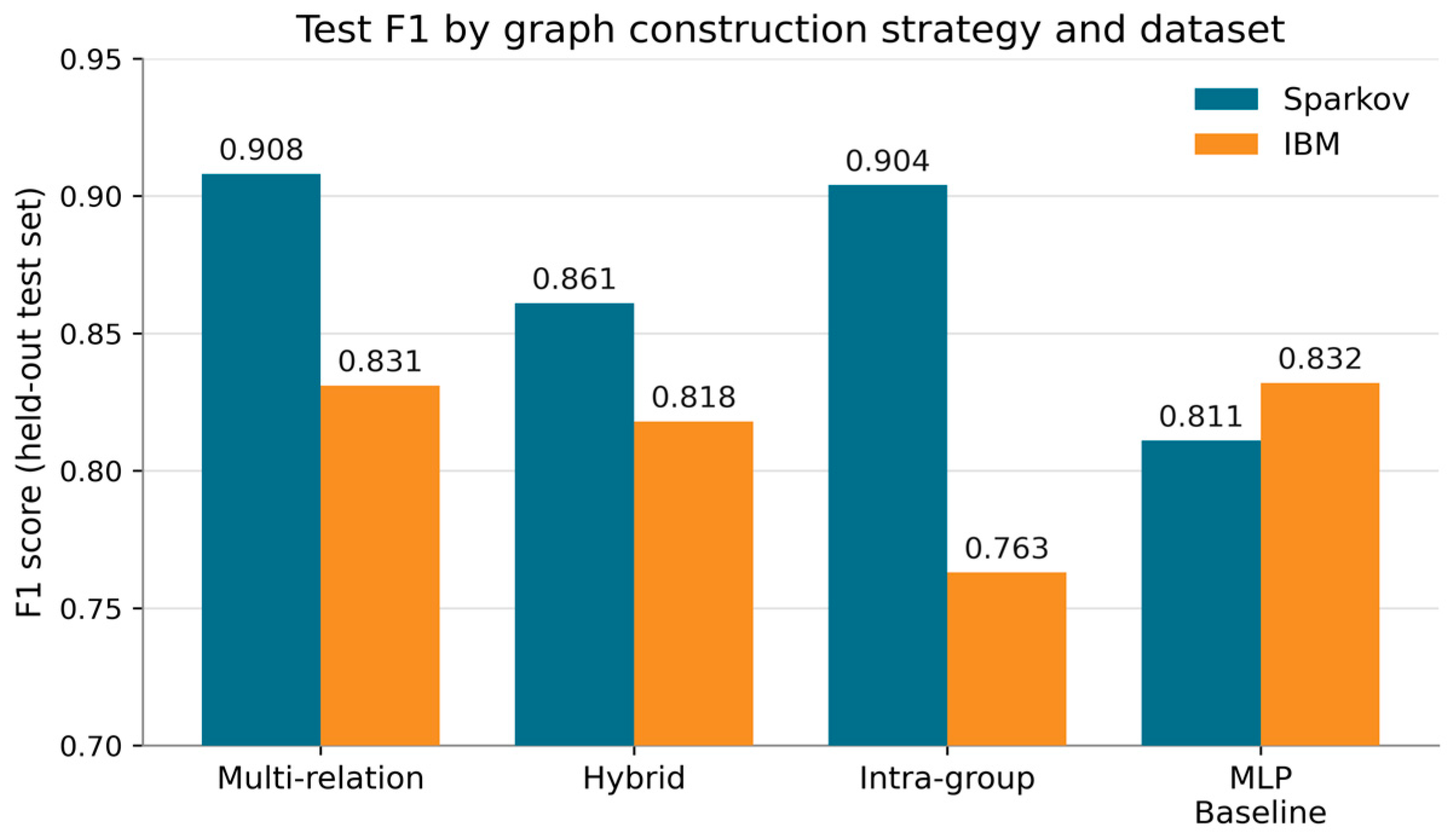Figure 4 visualises this pattern across both datasets: the MLP is the only strategy where IBM performance exceeds Sparkov, illustrating that topology’s advantage is conditional on graph density rather than universal.

Table 6. IBM confusion matrix analysis. TP: true positives; FP: false positives; FN: false negatives; TN: true negatives; FPR: false positive rate; FNR: false negative rate.

Strategy	TP	FP	FN	TN	FPR	FNR
Multi-relation	4467	601	1218	57,563	1.03%	21.4%
Hybrid	4384	649	1301	57,515	1.12%	22.9%
Intra-group	4397	1443	1288	56,721	2.48%	22.7%
MLP Baseline	4544	697	1141	57,467	1.20%	20.1%

reports the corresponding confusion matrices; intra-group’s markedly higher false positive rate (2.48% vs. 1.03–1.20% for the other strategies) is consistent with its collapse under sparse conditions.

5.4. Architecture Sensitivity

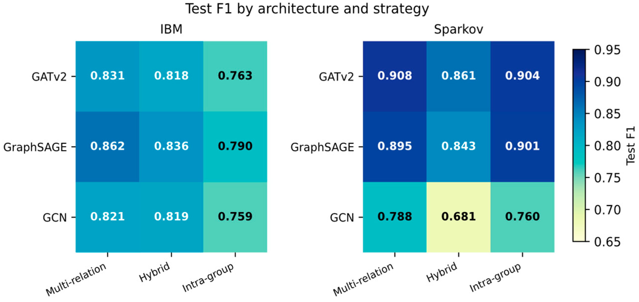
We test directly whether topology performance rankings are preserved when the GNN operator is swapped, re-running all three strategies with GCN and GraphSAGE in place of GATv2, holding every other component of the pipeline fixed. Figure 5 summarises the resulting F1 scores as a heatmap across all architecture–strategy–dataset combinations, with the same values reported numerically in

Table 7. Test F1 by architecture and strategy.

Dataset	Architecture	Multi-Rel	Hybrid	Intra-Grp
IBM	GATv2	0.831	0.818	0.763
IBM	GraphSAGE	0.862	0.836	0.790
IBM	GCN	0.821	0.819	0.759
Sparkov	GATv2	0.908	0.861	0.904
Sparkov	GraphSAGE	0.895	0.843	0.901
Sparkov	GCN	0.788	0.681	0.760

.

On IBM, the strategy ranking is fully consistent across all three architectures (multi-relation > hybrid > intra-group), with GraphSAGE achieving the highest absolute F1 of any architecture–strategy combination (0.862); on Sparkov, the ranking is not fully preserved, as GraphSAGE narrowly inverts the near-tied multi-relation/intra-group order (0.901 vs. 0.895), consistent with a near-tie rather than a genuine reordering given GATv2 itself shows the same closeness (0.908 vs. 0.904). The one finding that holds across every architecture tested is that hybrid is never the best-performing strategy on either dataset, regardless of architecture—FAISS similarity edges add noise relative to relational structure under every GNN variant tested. Architecture choice also affects absolute performance independently of topology: GCN underperforms GATv2 and GraphSAGE substantially on Sparkov (F1 = 0.681 vs. 0.861 for hybrid, an 18-point gap on the identical graph) but is far more competitive on IBM, even narrowly exceeding GATv2 on hybrid (0.819 vs. 0.818)—suggesting GCN’s weakness is tied to denser, more heterogeneous graphs rather than being a uniform architectural deficiency. Whether multi-relation exceeds the MLP baseline is itself architecture-dependent: on IBM (MLP F1 = 0.832), only GraphSAGE’s multi-relation strategy (0.862) exceeds the MLP outright, while GATv2 (0.831) and GCN (0.821) are essentially tied with or marginally below it. On Sparkov (MLP F1 = 0.811), multi-relation and intra-group both exceed the MLP under GATv2 and GraphSAGE, but GCN underperforms the MLP for both strategies (0.788 and 0.760 vs. 0.811). This indicates that the topology-adds-value finding from Section 5.2 is architecture-dependent rather than a universal property of the framework, and is most reliably observed under GraphSAGE and, on the denser Sparkov dataset, GATv2.

6. Comparison with Prior Work

Against prior work on the same datasets, Ref. [7] reports F1 = 0.71 on IBM using Edge-GCN, and [8] reports F1 = 0.854 using heterogeneous GAT on a proprietary simulated dataset distinct from Sparkov and IBM, both under coupled construction architecture settings without leakage-safe splits. Our multi-relation strategy achieves F1 = 0.831 and AUC = 0.985 on IBM under strictly controlled conditions.

Table 8. Performance comparison with prior work on the Sparkov and IBM datasets.

Method	Dataset	F1	P	R	AUC	Graph
TigerGraph [13]	Sparkov	0.773	0.828	0.724	—	Hetero
NeuraShield [7]	IBM	0.714	0.642	0.804	0.870	Hetero
Intra-grp work [11] GATv2	Sparkov	0.909	0.943	0.877	0.992	Homo
Intra-grp work [11] GATv2	IBM	0.763	0.771	0.756	0.962	Homo
Ours (multi-rel GATv2)	Sparkov	0.908	0.950	0.869	0.994	Homo
Ours (multi-rel GATv2)	IBM	0.831	0.881	0.786	0.985	Homo

Homo = homogeneous graph, Hetero = heterogeneous graph. Leakage-safe = group-stratified splitting + training-only feature normalisation enforced. — = not reported by authors.

summarises comparisons with prior work reporting results on Sparkov or IBM specifically; Ref. [8]’s result is excluded from this table since it is not evaluated on either dataset or is therefore not directly comparable. We report the intra-group strategy’s comparison against TigerGraph and NeuraShield specifically because it provides direct continuity with our own prior work [11], which evaluated only the intra-group formulation against these same baselines; Table 8 additionally reports multi-relation’s absolute performance alongside intra-group so that readers can compare either strategy directly against prior work. On Sparkov, our intra-group GATv2 strategy improves F1 by 16.9% over TigerGraph (0.904 vs. 0.773). On IBM, it outperforms NeuraShield in F1 (0.763 vs. 0.714, +6.9%) and precision (0.753 vs. 0.642, +17.3%), though NeuraShield achieves higher recall (0.804 vs. 0.773). These comparisons should be interpreted with caution, as the methods differ not only in graph construction but also in preprocessing, evaluation protocol, and model formulation. TigerGraph relies on heuristic thresholds and community detection rather than learned representations, making the comparison one of paradigm rather than architecture. NeuraShield uses a heterogeneous cross-entity graph with different node and edge definitions, and its reported metrics may reflect different train/test splits and class imbalance handling. No prior work on either dataset enforces group-stratified splitting or controlled down-sampling as applied here, which may affect the reported performance in either direction. Despite these differences, a consistent pattern emerges: the proposed method achieves competitive or superior performance when per-cardholder graph density is sufficient (Sparkov). A fully controlled comparison would require re-implementing all methods under identical preprocessing and evaluation conditions, which we identify as an opportunity for future benchmarking work. Down-sampling substantially eases the task: at native fraud rates (~0.1% Sparkov, ~0.09% IBM), fraud is roughly 1000× rarer than legitimate transactions, versus ~4:1 and ~10:1 after down-sampling. This easier class balance likely inflates our F1 relative to studies evaluated at native imbalance and should be weighed when interpreting Table 8.

7. Discussion

The MLP baseline serves as the controlled ablation condition: any GNN strategy that fails to exceed it cannot claim that graph topology contributes discriminative value beyond what the node features alone provide. Multi-relation temporal achieves the highest or near-highest GNN performance on both datasets (see Section 5), but the MLP baseline complicates this picture: on IBM, it marginally exceeds all GNN strategies in F1 while lagging in AUC and AP. This does not contradict the value of graph topology; it confirms that topology value is conditional on graph quality. On Sparkov, where graph construction yields dense, informative neighbourhoods (avg. degree 10.4–17.3, with hybrid’s FAISS-augmented graph the densest of the three despite not producing the highest F1), all GNN strategies exceed the MLP by 5.0–9.7 F1 points. On IBM, where sparse graphs limit neighbourhood aggregation (avg. degree 1.1–10.1), the F1 advantage disappears entirely: multi-relation essentially ties the MLP (0.831 vs. 0.832), while hybrid and intra-group fall further behind, though ranking advantages in AUC and AP persist for multi-relation and hybrid.

This divergence is threshold-driven rather than indicating weaker discrimination: the GNN strategies tune to higher thresholds than the MLP, which may reflect a shifted or more concentrated score distribution, though we did not formally assess calibration. With an average degree of just 1.1, intra-group’s GATv2 aggregation receives information from effectively one neighbour per node, making message passing close to, but not identical to, a feature lookup: its AUC (0.962) remains well above the MLP’s effective floor. For multi-relation (avg. degree 4.3), meaningful aggregation still occurs, explaining why ranking advantages persist even when F1 is marginal. Intra-group is the clearest victim of sparsity, falling 6.9 F1 points below the MLP, though its retained AUC indicates weakened, not complete, graph utility under near-self-loop conditions.

Architecture choice adds a further qualification: strategy rankings hold exactly on IBM across all three architectures tested, but GraphSAGE narrowly inverts the near-tied multi-relation/intra-group order on Sparkov. The one finding that holds identically across every architecture tested that hybrid never wins, on either dataset, is the most consistent topology-level result in this study, since it cannot be attributed to GATv2-specific inductive bias.

8. Limitations

This work has several limitations. Both Sparkov and IBM are simulated or synthetic datasets; neither reflects the full behavioural complexity, fraud pattern diversity, or transaction volume of a production payment system, and the results should be validated on real-world data before deployment. The down-sampling applied to both datasets (to the 18.4% and 9.09% fraud rates, respectively) alters graph density and class balance relative to natural fraud rates (0.1–1%), so the density-dependent effects reported here may not transfer directly to production-scale, highly imbalanced graphs. The framework was evaluated only with neighbourhood-aggregating GNN architectures (GATv2, GCN, GraphSAGE); other model families, such as heterogeneous or transformer-based graph models, were not tested and may respond differently to the same topologies. Finally, all reported metrics are single point estimates from one five-fold ensemble per configuration; we did not assess variance across random seeds, so close results such as the 0.004 F1 gap between multi-relation and intra-group on Sparkov should be interpreted as suggestive rather than statistically confirmed differences. Future work should repeat each configuration across multiple seeds and report variance or a paired significance test alongside point estimates. Finally, because the three construction strategies differ in edge density and edge type composition, as well as topology type, hybrid adds similarity edges on top of the multi-relation edge set, and intra-group restricts edges to within-cardholder scope, the reported effects should be read as differences between strategies as implemented, rather than as a pure isolation of topology from graph density; a density-matched ablation (e.g., degree-matched random rewiring within each strategy) would be needed to separate these factors more cleanly.

References

- Abdallah, A.; Maarof, M.A.; Zainal, A. Fraud detection system: A survey. J. Netw. Comput. Appl. 2016, 68, 90–113. [Google Scholar] [CrossRef] [Scilit]
- Liu, G.; Tang, J.; Tian, Y.; Wang, J. Graph Neural Network for Credit Card Fraud Detection. In Proceedings of the 2021 international Conference on Cyber Physical Intelligence (ICCSI), Beijing, China, 18–20 December 2021. [Google Scholar] [CrossRef] [Scilit]
- Cui, Y.; Han, X.; Chen, J.; Zhang, X.; Yang, J.; Zhang, X. FraudGNN-RL: A Graph Neural Network with Reinforcement Learning for Adaptive Financial Fraud Detection. IEEE Open J. Comput. Soc. 2025, 6, 426–437. [Google Scholar] [CrossRef] [Scilit]
- Maganti, S. When Graph Structure Becomes a Liability: A Critical Re-Evaluation of Graph Neural Networks for Bitcoin Fraud Detection under Temporal Distribution Shift. arXiv 2026, arXiv:2604.19514. [Google Scholar]
- Sajja, B. TravelFraudBench: A Configurable Evaluation Framework for GNN Fraud Ring Detection in Travel Networks. arXiv 2026, arXiv:2604.21093. [Google Scholar]
- Kabwama, C.A.; Businge, P.; Malingu, C.J.; Atuhaire, J.I.; Ankunda, I.A.; Ariho, J.G.; Mugalu, B.; Musinguzi, D. Graph attention networks for credit card fraud detection: A relational learning approach. World J. Adv. Res. Rev. 2025, 26, 2580–2585. [Google Scholar] [CrossRef] [Scilit]
- Gunawardana, P.; Samaraweera, W.J.; Meththananda, R.G.U.I. NeuraShield: A GNN Based Approach to Credit Card Fraud Detection. In Proceedings of the 2025 International Research Conference on Smart Computing and Systems Engineering (SCSE), Colombo, Sri Lanka, 3 April 2025. [Google Scholar] [CrossRef] [Scilit]
- Amuche, C.I. Multi-Relation Graph Transformer and Edge Aware Learning: A Scalable Approach for Detecting Fraud in Heterogeneous Graphs. In Proceedings of the International Conference on Software Engineering and Computer Science (CSECS), Taicang, China, 21–23 March 2025. [Google Scholar]
- Mardani, S.; Moradi, H. Using graph attention networks in healthcare provider fraud detection. IEEE Access 2024, 12, 132786–132800. [Google Scholar] [CrossRef] [Scilit]
- Zheng, Z.; Bochuan, Z.; Yuping, S. Temporal-aware graph attention network for cryptocurrency transaction fraud detection. arXiv 2025, arXiv:2506.21382. [Google Scholar]
- Amiri, R.; Jaf, S. Multi-Edge Intra-Group Graph Construction for Credit Card Fraud Detection. In Proceedings of the 31st International Conference on Automation and Computing, High Wycombe, UK, 26–28 August 2026. [Google Scholar]
- Huo, M.; Lu, K.; Zhu, Q.; Chen, Z. Enhancing customer contact efficiency with graph neural networks in credit card fraud detection workflow. In Proceedings of the 2025 IEEE 7th International Conference on Communications, Information System and Computer Engineering (CISCE), Guangzhou, China, 9–11 May 2025; pp. 320–324. [Google Scholar] [CrossRef] [Scilit]
- Mauliddiah, N.; Suharjito. Implementation Graph Database Framework for Credit Card Fraud Detection. Procedia Comput. Sci. 2023, 227, 326–335. [Google Scholar] [CrossRef] [Scilit]
- Johnson, J.; Douze, M.; Jégou, H. Billion-scale similarity search with GPUs. IEEE Trans. Big Data 2019, 7, 535–547. [Google Scholar] [CrossRef] [Scilit]
- Brody, S.; Alon, U.; Yahav, E. How Attentive are Graph Attention Networks? In Proceedings of the International Conference on Learning Representations (ICLR), Virtual Event, 25–29 April 2022. [Google Scholar]
- Kipf, T.; Welling, M. Semi-supervised classification with graph convolutional networks. In Proceedings of the International Conference on Learning Representations (ICLR), Toulon, France, 24–26 April 2017. [Google Scholar]
- Hamilton, W.L.; Ying, R.; Leskovec, J. Inductive Representation Learning on Large Graphs. In Proceedings of the 31st Conference on Neural Information Processing Systems (NeurIPS), Long Beach, CA, USA, 4–9 December 2017. [Google Scholar]
- Shenoy, K. Credit Card Transactions Fraud Detection Dataset. Kaggle. 2020. Available online: https://www.kaggle.com/datasets/kartik2112/fraud-detection (accessed on 19 August 2026).
- IBM Research. IBM Transactions for Anti Money Laundering (AML). Kaggle. 2023. Available online: https://www.kaggle.com/datasets/ealtman2019/ibm-transactions-for-anti-money-laundering-aml (accessed on 19 August 2026).
Figure 1.
Multi-relation temporal strategy. The same five transactions (T1–T5) are connected through three relational lenses: Card group (blue), Merchant (coral), Global time (dashed grey).
Figure 2.
Hybrid strategy. Domain-driven relational edges (left, solid) and data-driven FAISS k-NN similarity edges (right, dashed) over the same transaction set, merged into one homogeneous graph.
Figure 3.
Intra-group strategy. Each cardholder forms an isolated subgraph with temporal chains (green), similarity edges (dashed), and merchant sub-chains (coral, dotted). No edges cross cardholder boundaries.
Figure 4.
Test F1 by graph construction strategy across both datasets. Topology provides a clear advantage on Sparkov (dense graphs) but the advantage narrows or reverses on IBM (sparse graphs), where the MLP baseline becomes competitive.
Figure 5.
Test F1 by architecture and graph construction strategy. Intra-group is consistently the weakest strategy under sparse conditions (IBM); hybrid is never the strongest strategy under any architecture on either dataset.