PASM-Net: A Coordinate-Aware Manifold-Regularized Framework for Open-Set UAV RF Fingerprint Identification

Abstract

To address the challenges of classifying known categories and rejecting unknown categories in the radio-frequency fingerprinting of uncooperative UAVs in open, low-altitude environments, this paper proposes PASM-Net, an open-set recognition method based on coordinate awareness and manifold continuity regularization. Existing deep learning-based RFFI methods still suffer from two shortcomings in open scenarios: First, while conventional convolutions and global pooling yield compact representations, they may weaken position-related information in the time–frequency spectrum, thereby affecting the model’s ability to characterize frequency-hopping trajectories and local time–frequency structures; on the other hand, decision mechanisms that rely solely on Softmax classifiers or simple distance metrics are susceptible to signal amplitude fluctuations and intra-class distribution dispersion, leading to the misclassification of unknown samples into known classes. To address these issues, this paper designs the PASM-Net feature-learning framework. First, the model employs multiscale hollow convolutions to extract local time–frequency features across different receptive fields and introduces a coordinate attention mechanism (Coordinate Attention, CoordAtt) prior to global pooling, thereby enhancing the model’s ability to represent position-related information in both the time and frequency domains. Second, the model introduces manifold continuity regularization (MCR) in the fused semantic space. By constraining feature variations within local neighborhoods via a Laplacian regularization term, MCR reduces the dispersion of known-class feature distributions. Finally, the model employs ArcFace to enhance the angular separability among known classes and performs open-set classification based on the cosine distance between test samples and the centers of known classes. The experimental results across six open-set scenarios on the DroneRFb-Spectra dataset showed that PASM-Net achieved an average true unknown rate (TUR) of 99.48%, an unknown accuracy of 97.9%, and an unknown-class precision (UP) of 87.3%, while maintaining a high performance in known-class recognition. Under the current experimental setup, this effectively improves the trade-off between known-class classification and unknown-class rejection.

1. Introduction

With the rapid increase in the number of commercial drones, monitoring non-cooperative targets in low-altitude airspace has become a core national security challenge. Given their impressive performance in modern warfare [1], efficiency in logistics and transportation [2], convenience in environmental monitoring [3], and pivotal role in the low-altitude economy [4], the airspace security challenges they pose have transcended the scope of traditional regulation. Among the various drone monitoring methods—such as vision-based imaging [5], Doppler radar [6], and hybrid approaches [7]—many are susceptible to interference from weather conditions and other flying objects. Passive radio frequency fingerprint identification (RFFI) technology, with its high stealth and ability to operate beyond the line of sight (NLoS), is gradually replacing optical and acoustic [8] solutions and becoming the cornerstone of an all-weather defense system. Radio frequency fingerprint identification (RFFI) aims to identify the identity of UAV transmitters by utilizing unique signal characteristics in the transmitter’s RF front end that result from device-manufacturing variations, hardware non-idealities, and changes in the operating conditions [9].

RF fingerprinting exploits the inherent hardware characteristics of individual transmitters, arising from manufacturing variations and component parameter deviations, as unique signatures for identification, providing a lightweight and secure solution for UAV authentication. Early research focused on building an RF database for drones and validating the effectiveness of deep learning methods. For example, Al-Sa’d et al. systematically collected RF signals from various drones in different flight modes and used deep neural networks for detection and identification. They preliminarily demonstrated the feasibility of using RF signals for drone identification and contributed to the development of an open-source database [10]. Basak et al. created a multi-signal dataset comprising nine types of commercial drones. They compared the performance of a YOLO-based joint detection–classification framework with a two-stage method, providing a reference for drone perception in complex scenarios [11]. Subsequently, Cai incorporated manifold regularization and cross-domain learning, significantly improving the drone recognition performance in closed-set scenarios [12].

However, traditional RFFI methods typically rely on the closed-set assumption, meaning that the category of a test sample must appear in the training set. This is unrealistic in actual open environments, where unauthorized drones of unknown models may be misclassified as known categories, posing serious security risks. Therefore, open-set recognition has become a critical bottleneck that must be addressed to advance RFFI toward practical applications. The goal of open-set recognition is to accurately classify known categories while effectively detecting and rejecting samples from unknown categories. Open-set recognition is closely related to out-of-distribution (OOD) detection, which aims to handle samples belonging to classes not encountered during training. Early work, such as OpenMax [13] proposed by Bendale et al., estimated the probability that an input sample belongs to an unknown class by calibrating the activation vectors of the SoftMax layer, providing a foundational framework for the open-set adaptation of deep networks. Wang et al. conducted a systematic analysis and evaluation of OOD detection and OSR, pointing out that their performance is strongly correlated and that scoring rules sensitive to the amplitude of deep features typically perform better, providing important insights for the design of open-set methods [14].

In response, researchers have proposed various solutions. Among these, the prototype-based learning paradigm is naturally suited for open-set tasks because it can learn compact intra-class representations and expand inter-class boundaries. Mao et al. proposed a method for few-sample open-set drone recognition based on a multi-domain prototype network that fuses time- and frequency-domain features via a self-attention mechanism and constructs a decision boundary in Euclidean distance space [15]. Xie et al. introduced Gaussian prototypes and Mahalanobis distance, proposing a meta-learning Gaussian prototype network that enhances the open-set performance under few-sample conditions through a designed open-set loss function [16]. Yan et al. further designed TASE-Net, combining a transformer-enhanced SE module with a Gaussian mixture model to perform open-set few-sample recognition using robust features constructed from the cyclic spectrum [17]. In addition, new paradigms based on relational reasoning have been proposed, such as the RAD framework by Fu et al., which distinguishes between known and unknown objects by inferring the relationships among discriminative regions and can semantically group detected unknown samples to explore information about new classes [18]. In the radar modality, Mei et al. utilized high-resolution range images to constrain the feature space via a range loss and fit Weibull distribution boundaries to achieve the open-set recognition of UAVs [19].

To address the open-set recognition (OSR) problem in UAV radio-frequency fingerprinting, models must not only accurately distinguish known UAV classes during training, but also identify unseen targets during testing. Existing deep learning methods typically employ convolutional feature extraction, global pooling, and Softmax classifiers to perform closed-set recognition; however, they still suffer from two shortcomings in open scenarios.

First, time–frequency–location-related information is weakened during the global aggregation process. The discriminative features of UAV RF signals are not only reflected in the intensity of local time–frequency textures; they are also related to frequency-hopping trajectories, temporal evolution patterns, and local time–frequency structures. While applying global average pooling directly to convolutional features can yield a compact representation and enhance the translation robustness to some extent, certain fine-grained responses related to temporal and frequency positions may be averaged out, thereby weakening the model’s ability to characterize weak RF fingerprint features.

Second, the discriminative boundary in open scenarios is prone to instability. In real-world low-altitude monitoring scenarios, the received signals are affected by factors such as the transmission distance, channel fading, and ambient noise, leading to some dispersion among signals from drones of the same type in the feature space. If the model relies solely on a Softmax classifier or a simple Euclidean distance metric, it may produce a wide decision boundary around known classes, leading to high-confidence misclassifications of unknown samples. Therefore, open-set recognition models need to maintain the separability of known classes while further enhancing the feature compactness and constructing a more stable rejection boundary for unknown samples.

To address the above issues, this paper proposes PASM-Net, an open-set recognition network that incorporates coordinate-aware and manifold continuity regularization. Rather than simply removing global pooling, this network introduces position-aware and sequence-modeling mechanisms prior to global semantic compression to enhance the model’s ability to represent spatiotemporal structural information. Its main contributions are as follows:

(1)

Coordinate-aware multiscale spatiotemporal feature extraction. This paper first employs a multiscale hollow convolution branch to extract local time–frequency texture features across different receptive fields. Subsequently, a coordinate attention mechanism (Coordinate Attention, CoordAtt) is introduced prior to global pooling to aggregate contextual information along both the time and frequency dimensions, generating position-related attention weights to recalibrate the multiscale features. This design mitigates the weakening of spatiotemporal positional information caused by direct global aggregation, thereby enhancing the model’s ability to represent frequency-jump trajectories and local spatiotemporal structures.

(2)

Fusion of local time–frequency features and global sequence dependencies. In addition to the two-dimensional time–frequency map branch, this paper further constructs time-series and frequency-series modeling branches to capture global dependencies of the signal across the temporal and frequency dimensions via positional encoding and transformer encoders. Subsequently, the semantic features obtained from the local spatial branch and the sequence branches were fused to obtain a more comprehensive representation of the UAV RF fingerprint.

(3)

Manifold continuity regularization. To enhance the local consistency of feature distributions within known classes, this paper introduces manifold continuity regularization (MCR) in the fused semantic space. This module constructs a k-nearest-neighbor graph from in-batch samples. It uses a Tulaplas regularization term to constrain feature variation within local neighborhoods, thereby encouraging adjacent samples to maintain a smooth distribution in semantic space. This constraint helps reduce the discretization of known-class features, providing a more stable feature foundation for subsequent open-set threshold decision-making.

(4)

Hypersphere angular metric and open-set threshold decision-making. This paper uses the ArcFace classification head to normalize features and class weights and to enhance the separability between known classes via angular distance. During inference, the model makes classifications based on the cosine distance between the normalized semantic features and the centers of known classes, and estimates class thresholds using the training set’s distance distribution. When the distance from a test sample to the centers of all known classes exceeds the corresponding threshold, the sample is classified as an unknown class. This strategy reduces the impact of feature amplitude fluctuations on classification boundaries and enhances the model’s ability to reject unknown samples in open scenarios.

2. Definition of Signal Expression and Recognition Problems in Open Environments

In non-cooperative UAV monitoring scenarios, the RF signals received by the receiver are typically affected by factors such as transmitter hardware variations, wireless channel propagation, environmental noise, and co-channel interference. Unlike in traditional closed-set classification, unknown UAV classes not encountered during training may also appear in open environments. Therefore, an RFFI open-set classification model must not only accurately distinguish between known UAV classes, but also effectively reject samples from unknown classes. This section first presents a radio frequency signal observation model and a time–frequency representation for non-cooperative environments, followed by a definition of the open-set recognition problem and its decision objective. It should be noted that this paper does not explicitly estimate or eliminate environmental interference terms; instead, it treats them as interference factors in an open electromagnetic environment and mitigates their impact on the recognition boundary through subsequent feature learning and open-set threshold decision-making.

2.1. Modeling of Non-Cooperative RF Signals and Their Time–Frequency Representation

In actual low-altitude monitoring scenarios, the RF signals from drones captured by the receiver are not ideal hardware fingerprint signals, but rather observations affected by a combination of channel propagation, noise, and co-channel interference. Let $s_i\left(t\right)$ denote the ideal baseband signal transmitted by a Class i UAV, and let ${\Phi }_i(·)$ denote the non-ideal mapping caused by variations in the transmitter’s RF front-end hardware, such as power amplifier nonlinearity, I/Q imbalance, and local oscillator offset. Let $h(t,\tau )$ denote the time-varying channel impulse response, $n\left(t\right)$ denote background noise, and $j\left(t\right)$ denote co-channel or adjacent-channel interference terms. Then, the observed signal at the receiver can be expressed as:

$$y\left(t\right)=\int h(t,\tau ){\Phi }_i\left(s_i(t-\tau )\right)d\tau +j\left(t\right)+n\left(t\right)$$

(1)

In this context, $n\left(t\right)$ may include additive white Gaussian noise or colored noise. At the same time, $j\left(t\right)$ may represent structured interference from Wi-Fi, Bluetooth, other drone remote-control signals, or multiple drones operating simultaneously. This paper does not explicitly estimate or separate $j\left(t\right)$; instead, it treats it as an external disturbance in an open electromagnetic environment and mitigates its impact on the recognition performance by learning robust feature representations and employing open-set classification mechanisms.

To convert one-dimensional time-domain signals into a two-dimensional representation better suited to processing by deep neural networks, this paper employs the short-time Fourier transform (STFT) to obtain time–frequency spectra. The discrete STFT can be expressed as:

$$X(\tau ,k)={\displaystyle \sum _{n=0}^{N-1}}y\left[n\right]w[n-\tau ]e^{-j2\pi kn/N}$$

(2)

Here, $w[·]$ denotes the window function, $\tau$ the time-frame index, and k the frequency index. Next, a logarithmic transform is applied to the amplitude spectrum to obtain a two-dimensional time–frequency representation:

$$S(\tau ,k)=log\left(\right|X(\tau ,k){|}^2+ϵ)$$

(3)

Here, $ϵ$ is a small constant used to prevent numerical instability. Ultimately, each sample is represented as a two-dimensional time–frequency tensor of uniform dimensions and fed into the subsequent network for feature learning.

For drone RF signals, such as frequency-hopping spread spectrum, discriminative information is reflected not only in the intensity of local time–frequency textures, but also in frequency-hopping trajectories, local time–frequency structures, and temporal evolution patterns. If global spatial aggregation is performed directly on the convolutional features, some location-dependent fine-grained responses may be averaged out, thereby weakening the model’s ability to characterize weak RF fingerprint features. Therefore, this paper introduces a coordinate attention mechanism prior to global semantic compression to enhance the network’s ability to perceive positional information in the time and frequency domains.

2.2. Definition of the Set-Opening Recognition Problem

In closed-set classification tasks, the training set and test set typically share the same class space. However, in non-cooperative drone monitoring scenarios, the system may encounter drones of unknown models that were not present during training. Therefore, the model must not only classify known classes, but also determine whether an input sample belongs to an unknown class.

Let the known class space be: ${\mathcal{Y}}_K=\{1,2,\dots ,k\}$; the unknown category spaces are: ${\mathcal{Y}}_U$, Specifically, ${\mathcal{Y}}_K\cap {\mathcal{Y}}_U=\varnothing$.

During the training phase, data can only be obtained from known categories:

$${\mathcal{D}}_{train}=\{(x_i,y_i)\mid y_i\in {\mathcal{Y}}_K\}$$

(4)

The goal of open-set recognition is to learn a feature-mapping function $f_{\theta }(·)$ and a decision function $g(·)$ such that, during the testing phase, the model can correctly classify samples of known classes while classifying samples from ${\mathcal{Y}}_U$ as unknown classes.

In this paper, the input samples are first mapped to semantic features:

$$z=f_{\theta }\left(x\right)$$

(5)

For a known class c, let its class center be denoted as ${\mu }_c$. During the inference stage, this paper uses the cosine distance between the normalized features and the class center as the basis for open-set classification:

$$d_c\left(z\right)=1-cos(z,{\mu }_c)$$

(6)

If the distance from a test sample to all known class centers is greater than the corresponding class threshold, the sample is classified as an unknown class:

$$g\left(x\right)=\left\{\begin{array}{cc}arg{min}_c{d}_c\left(z\right),\hfill & \mathrm{if}{min}_c(d_c\left(z\right)-{\theta }_c)\le 0,\hfill \\ unknown,\hfill & \mathrm{otherwise}.\hfill \end{array}\right.$$

(7)

Here, ${\theta }_c$ refers to the class threshold estimated based on the distance distribution of known training or validation samples. This decision-making approach avoids relying solely on the maximum probability from Softmax to determine unknown classes, enabling the rejection of unknown samples based on the distance distribution in the feature space.

3. The PASM-Net Method

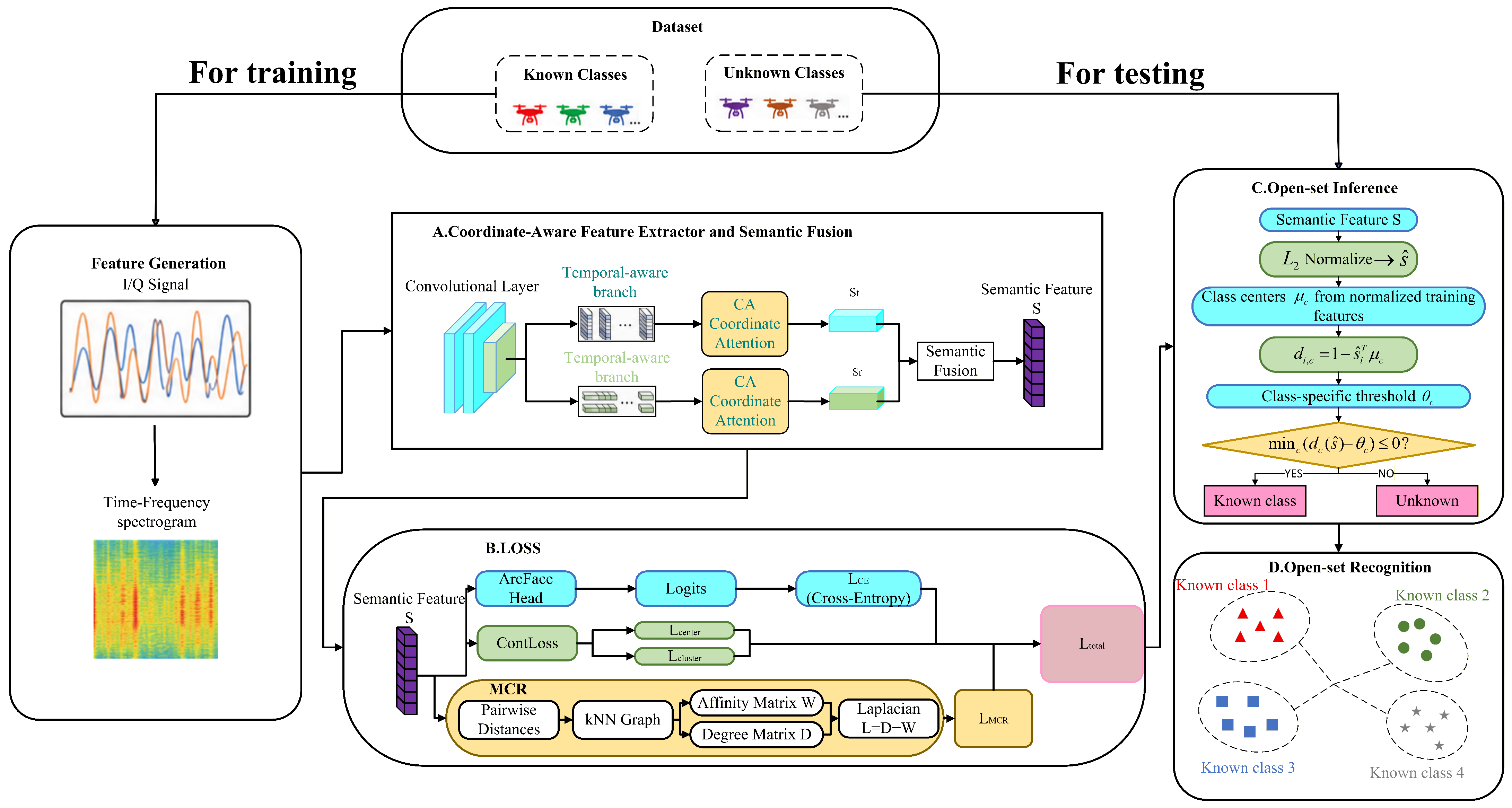
To improve the stability of known-class classification and unknown-class rejection in the open-set recognition of UAV radio-frequency fingerprints, this paper proposes the framework of PASM-Net, a coordinate-aware and manifold-continuity regularization network. The overall architecture is shown in Figure 1. The network primarily consists of four components: a multiscale time–frequency feature extraction module, a coordinate attention module, a time–frequency sequence-modeling branch, and a semantic feature-learning module for open-set decision-making.

Specifically, PASM-Net first uses multiscale hollow convolutions to extract the local time–frequency texture features across different receptive fields. It then introduces CoordAtt before global pooling to model contextual information in the temporal and frequency domains, thereby enhancing the model’s ability to represent position-dependent features. Subsequently, the model constructs temporal and frequency-sequence branches to capture global dependencies using positional encoding and a transformer encoder. Finally, the three semantic feature streams are fused and fed into the ArcFace classification head for training, incorporating manifold continuity regularization to constrain the feature distribution of known classes. During the inference stage, the model performs a classification of known classes and the rejection of unknown classes based on the cosine distance between the test sample and the center of the known class, along with a class threshold.

3.1. Multiscale Time–Frequency Feature Extraction and Coordinate Attention

In time–frequency plots, drone RF signals typically manifest as a combination of local textures, frequency-jump trajectories, and temporal evolution patterns. Single-scale convolution struggles to capture both fine-grained local textures and larger-scale time–frequency structures simultaneously. To address this, this paper constructs a multiscale hollow convolution module within the two-dimensional time–frequency map branch, employing parallel convolution branches with expansion ratios of 1, 3, and 5 to extract time–frequency features across different receptive fields. The three convolution outputs are concatenated along the channel dimension to obtain a multiscale feature representation:

$$F_{ms}=\mathrm{Concat}(F_{d=1},F_{d=3},F_{d=5})$$

(8)

In particular, $F_{d=1}$, $F_{d=3}$, and $F_{d=5}$ represent the output characteristics of the branches with different expansion rates.

Since applying global average pooling directly to two-dimensional convolutional features may weaken the positional information in the temporal and frequency dimensions, this paper introduces a coordinate attention mechanism (Coordinate Attention, CoordAtt) prior to global pooling. Unlike directly compressing two-dimensional features into a single global vector, CoordAtt performs one-dimensional context aggregation separately along the temporal and frequency directions, thereby preserving information in one spatial direction while obtaining a global response in the other. For an input feature $F_{ms}\in {\mathbb{R}}^{C\times H\times W}$, its aggregation along the frequency and time directions can be expressed as:

$$z_c^h\left(h\right)={\displaystyle \frac{1}{W}}{\displaystyle \sum _{w=1}^W}{F}_{ms,c}(h,w),z_c^w\left(w\right)={\displaystyle \frac{1}{H}}{\displaystyle \sum _{h=1}^H}{F}_{ms,c}(h,w)$$

(9)

In this context, $z_c^h\left(h\right)$ and $z_c^w\left(w\right)$ represent the one-dimensional features of the c-th channel along the temporal and frequency coordinate directions, respectively. Specifically, $z_c^h\left(h\right)$ is obtained by averaging along the w-dimension while preserving the coordinate h, whereas $z_c^w\left(w\right)$ is obtained by averaging along the h-dimension while preserving the coordinate w. The features from the two directions are then concatenated and passed through a $1\times 1$ convolution, batch normalization, and a nonlinear activation function to generate an intermediate representation:

$$q=\delta \left(\mathrm{BN}\left({\mathrm{Conv}}_{1\times 1}\left([z^h,z^w]\right)\right)\right)$$

(10)

Here, $\delta (·)$ denotes the $\mathrm{h}-\mathrm{swish}$ activation function. We further decompose q into attention weights in the time and frequency domains:

$$a^h=\sigma \left({\mathrm{Conv}}_{1\times 1}\left(q^h\right)\right),a^w=\sigma \left({\mathrm{Conv}}_{1\times 1}\left(q^w\right)\right)$$

(11)

Finally, the input features are re-scaled using attention weights in two directions:

$$\tilde{F}=F_{ms}\odot a^h\odot a^w$$

(12)

This process does not completely replace global average pooling; rather, it performs a location-dependent recalibration of multiscale time–frequency features prior to global pooling. After processing with CoordAtt, this paper then employs global average pooling and fully connected mapping to obtain spatial branch semantic features:

$$s_x=P_x\left(\mathrm{GAP}\left(\tilde{F}\right)\right)$$

(13)

3.2. Time and Frequency Series Modeling Branch

The 2D time–frequency plot branch primarily focuses on local spatial textures and coordinate-correlated responses. To further supplement the global dependency information, PASM-Net simultaneously constructs a time-series branch and a frequency-series branch. For the time–frequency spectrum S, this paper treats it as two separate sequence inputs along the time and frequency dimensions, namely the time series Y and the frequency series Z. These two types of sequences are first transformed via linear mapping into a unified-dimensional representation:

$$E_y=P_y\left(Y\right),E_z=P_z\left(Z\right)$$

(14)

In our implementation, both the temporal and frequency branches adopt the same transformer encoder configuration. Each sequence is first projected to a 64-dimensional embedding through two linear layers with an intermediate dimension of 128. Each transformer encoder consists of three stacked encoder layers with eight self-attention heads, a model dimension of $d=64$, and a feed-forward dimension of $d_{\mathrm{ff}}=256$. The two branches use separate transformer encoders with the same architectural configuration.

Given that the transformer encoder does not explicitly incorporate sequence position information, this paper introduces sinusoidal position encoding into the input:

$$\begin{array}{c}{\mathrm{PE}}_{(pos,2i)}=sin\left({\displaystyle \frac{pos}{{\mathrm{10,000}}^{2i/d}}}\right),\\ {\mathrm{PE}}_{(pos,2i+1)}=cos\left({\displaystyle \frac{pos}{{\mathrm{10,000}}^{2i/d}}}\right)\end{array}$$

(15)

Next, the sequence with the position encoding added is fed into the transformer encoder (TransEnc):

$$H_y=\mathrm{TransEnc}(E_y+{\mathrm{PE}}_y),H_z=\mathrm{TransEnc}(E_z+{\mathrm{PE}}_z)$$

(16)

Finally, the outputs of the two sequence branches are flattened and mapped to the semantic space, yielding the temporal branch semantic features $s_y$ and the frequency branch semantic features $s_z$:

$$s_y=P_{sy}\left(H_y\right),s_z=P_{sz}\left(H_z\right)$$

(17)

The semantic features from the three channels are then fused:

$$s=P_f\left([s_x,s_y,s_z]\right)$$

(18)

Here, $\left[·\right]$ denotes feature concatenation, and $P_f(·)$ denotes the semantic fusion mapping. The fused feature s serves as a unified semantic representation for subsequent classification, manifold regularization, and open-set classification.

3.3. Manifold Continuity Regularization

In open-set classification tasks, only samples from known classes are available during training. If the feature distributions of the known classes are too dispersed, the model is prone to incorrectly classifying unknown samples as belonging to a known class during testing. To enhance the local consistency of feature distributions for known classes, this paper introduces manifold continuity regularization (MCR) in the fused semantic space.

This paper treats it as a local smoothing constraint based on Tulaplas, used to reduce the feature variability among samples within a batch. Given a fused semantic feature matrix in a training batch:

$$S={[s_1,s_2,\dots ,s_B]}^T\in {\mathbb{R}}^{B\times d}$$

(19)

Here, B represents the batch size and d represents the dimension of the semantic features. First, the Euclidean distances between samples within a batch are calculated, and K nearest neighbors are selected for each sample. An adjacency matrix is constructed based on the Gaussian kernel function:

$$W_{ij}=\left\{\begin{array}{cc}exp\left(-{\displaystyle \frac{\parallel s_i-s_j{\parallel }_2^2}{2{\sigma }^2}}\right),\hfill & j\in {\mathcal{N}}_K\left(i\right)\hfill \\ 0,\hfill & \mathrm{otherwise}.\hfill \end{array}\right.$$

(20)

Here, ${\mathcal{N}}_K\left(i\right)$ denotes the set of K nearest neighbors of sample $s_i$, and $\sigma$ is the width of the Gaussian kernel. To obtain a symmetric neighborhood relationship, this paper applied a symmetrization operation to W:

$$W\leftarrow {\displaystyle \frac{W+W^T}{2}}$$

(21)

Next, the degree matrix is defined:

$$D_{ii}=\sum _j{W}_{ij}$$

(22)

This yields the Turaplas matrix:

$$L=D-W$$

(23)

MCR loss is defined as:

$${\mathcal{L}}_{MCR}={\displaystyle \frac{1}{B}}Tr\left(S^{T}LS\right)$$

(24)

This regularization term encourages samples in a local neighborhood to have similar representations in semantic space, thereby reducing local feature dispersion within known classes. Compared to the original classification loss, MCR primarily serves as a constraint on the feature space during training; during inference, the model no longer constructs a K-nearest-neighbor graph or computes the graph’s Laplacian matrix.

3.4. Intelligent UAV Frequency-Hopping Signal Detection Technology Algorithm

To mitigate the impact of variations in the feature amplitude on classification boundaries, this paper employed the ArcFace classification head for supervised training on known classes. ArcFace first performs an $L_2$ normalization on the semantic features $s_i$ and classifier weights $W_j$, ensuring that the classification logits are primarily determined by angular similarity:

$$cos{\theta }_j=W_j^T{s}_i$$

(25)

For the true class $y_i$, ArcFace introduces an additional angle interval m in angle space and adjusts the magnitude of the logits using a scaling factor r:

$${\mathrm{logit}}_{y_i}=rcos({\theta }_{y_i}+m),{\mathrm{logit}}_j=rcos\left({\theta }_j\right),j\ne y_i$$

(26)

The corresponding ArcFace cross-entropy loss is:

$${\mathcal{L}}_{Arc}=-{\displaystyle \frac{1}{N}}{\displaystyle \sum _{i=1}^N}log{\displaystyle \frac{e^{rcos({\theta }_{y_i}+m)}}{e^{rcos({\theta }_{y_i}+m)}+{\sum }_{j\ne y_i}{e}^{rcos{\theta }_j}}}$$

(27)

It is important to emphasize that ArcFace enhances the angular distinguishability between known classes, rather than detecting unknown classes on its own. In this paper, unknown class rejection was performed during the inference stage based on the cosine distance from semantic features to the centers of known classes.

Although the ArcFace loss improves the inter-class separability through angular margin constraints, additional feature regularization is required to further enhance the intra-class compactness. Therefore, two complementary regularization terms, i.e., center loss and cluster loss, are introduced to minimize intra-class feature variations and promote more discriminative feature clustering.

$${\mathcal{L}}_{center}={\displaystyle \frac{1}{2}}{\displaystyle \sum _{i=1}^N}{\parallel s_i-c_{y_i}\parallel }_2^2$$

(28)

where $s_i$ denotes the learned feature representation of the i-th sample and $c_{y_i}$ represents the center of the class to which the sample belongs.

$${\mathcal{L}}_{cluster}={\displaystyle \frac{1}{N}}\sum _i{∥s_i-c_{y_i}∥}_2^2$$

(29)

After training is complete, the semantic features of the training samples are first normalized and then the class centers for each known class are calculated:

$${\mu }_c={\displaystyle \frac{\frac{1}{N_c}{\sum }_{i:y_i=c}{\widehat{s}}_i}{{∥\frac{1}{N_c}{\sum }_{i:y_i=c}{\widehat{s}}_i∥}_2}},{\widehat{s}}_i={\displaystyle \frac{s_i}{\parallel s_i{\parallel }_2}}$$

(30)

For each known class c, the class-specific threshold ${\theta }_c$ is estimated from the intra-class angular distance distribution of the training samples. Specifically, after the L2 normalization, the cosine distance between each training feature and its corresponding class center is calculated as:

$$d_{i,c}=1-{\widehat{s}}_i^T{\mu }_c,$$

(31)

where ${\widehat{s}}_i$ denotes the normalized feature representation and ${\mu }_c$ represents the center of class c.

Based on the obtained distance distribution $D_c=\left\{d_{i,c}\right\}$, the threshold ${\theta }_c$ is determined according to the three-sigma criterion. Specifically, the largest distance within the three-standard-deviation range of the class-specific distance distribution is selected as the decision threshold:

$${\theta }_c=max\{d_{i,c}\mid d_{i,c}\le 3{\sigma }_c\},$$

(32)

where ${\sigma }_c$ denotes the standard deviation of the distance distribution of class c. This adaptive threshold estimation strategy removes the influence of extreme intra-class outliers while preserving the characteristic distribution of each known class.The final open-set decision follows Equation (7), where z is replaced by the normalized semantic feature $\widehat{s}$.

This decision-making approach avoids relying solely on the maximum Softmax probability for unknown sample rejection, enabling open-set recognition to exploit the class-specific distance distributions in the feature space.

4. Experimental Results and Analysis

This chapter evaluates the open-set recognition performance of PASM-Net using the DroneRFb-Spectra dataset [20]. This dataset was collected using USRP and contains RF signals from 24 types of micro drones, covering multiple brands such as DJI and FrSky, across frequency bands including 915 MHz, 2.4 GHz, and 5.8 GHz. In this paper, the raw I/Q signals were converted into two-dimensional time–frequency spectra and uniformly resized to a $512\times 512$ input tensor. The experiments primarily evaluated the model’s performance in known-class classification, unknown-class rejection, openness variations across multiple scenarios, and module ablation.

4.1. Experimental Design

The training and inference processes of PASM-Net are shown in Algorithm 1. During the model-training phase, only samples of known classes are used to learn the semantic feature space through the joint optimization of the ArcFace cross-entropy loss, center loss, clustering loss, and manifold continuity regularization loss. During the inference phase, the model first extracts normalized semantic features from the test samples, then calculates their cosine distances to the centers of each known class, and finally performs a classification into known classes or the rejection of unknown classes based on class thresholds.

The training parameters are shown in

Table 1. Training operation parameters.

Hyper-Parameter	Default Setup
Optimizer	Adam
Max Epoch	200
Batch Size	32
Learning Rate ($\alpha$)	$1\times {10}^{-4}$
Weight Decay	$1\times {10}^{-4}$
Semantic Dimension (D)	128
Margin ($m_c$)	8
${\eta }_1$ (Center Loss Weight)	0.05
${\eta }_2$ (Cluster Loss Weight)	1.0
${\eta }_3$ (ArcFace-CE Loss Weight)	1.0
${\eta }_4$ (MCR Loss Weight)	0.01
ArcFace Scale (s)	30.0
ArcFace Margin ($m_{arc}$)	0.5
MCR Neighbors ($K_m$)	5
MCR Gaussian Kernel ($\sigma$)	1.0

. The experiments used the Adam optimizer with a learning rate of $1\times {10}^{-4}$, a batch size of 32, and 128 semantic feature dimensions. Note that $m_c=8$ in the table refers to the interval parameter in the center/cluster constraint, whereas the angle interval in ArcFace is denoted as $m_{arc}=0.5$; these terms have different meanings.

Algorithm 1 Proposed PASM-Net for RF-based UAV open-set recognition.

Input: Training set ${\mathcal{D}}_{\mathrm{train}}={\left\{(X_i,Y_i,Z_i,c_i)\right\}}_{i=1}^N$, where $c_i\in \mathcal{K}=\{1,2,\dots ,K\}$; feature extractor $E(·;\Theta )$; ArcFace classification head $A(·;W)$; loss weights ${\eta }_1,{\eta }_2,{\eta }_3,{\eta }_4$; MCR neighbor number $K_m$; ArcFace scale s; ArcFace margin $m_{\mathrm{arc}}$. Output: Predicted label ${\widehat{y}}_t\in \mathcal{K}$ or ${\widehat{y}}_t=-1$.

Stage I: Feature learning Initialize network parameters $\Theta$ and ArcFace weights W. Randomly select a mini-batch from ${\mathcal{D}}_{\mathrm{train}}$. Extract semantic features: $$S=E(X,Y,Z;\Theta ).$$ Compute ArcFace logits: $$\widehat{y}=A(S,c;W).$$ Compute the ArcFace cross-entropy loss: $${\mathcal{L}}_{\mathrm{Arc}\text{-}\mathrm{CE}}=\mathrm{CE}(\widehat{y},c).$$ Compute center loss ${\mathcal{L}}_{center}$, cluster loss ${\mathcal{L}}_{cluster}$, and MCR loss ${\mathcal{L}}_{\mathrm{MCR}}$. Optimize the total objective: $${\mathcal{L}}_{\mathrm{total}}={\eta }_3{\mathcal{L}}_{\mathrm{Arc}\text{-}\mathrm{CE}}+{\eta }_1{\mathcal{L}}_{\mathrm{center}}+{\eta }_2{\mathcal{L}}_{\mathrm{cluster}}+{\eta }_4{\mathcal{L}}_{\mathrm{MCR}}.$$ Update $\Theta$ and W by back-propagation. Stage II: Open-set decision 9. Extract $L_2$-normalized semantic features ${\widehat{\mathbf{s}}}_i$ for all training samples. 10. For each known class $k\in \mathcal{K}$, compute the normalized class center: $${\mathit{\mu }}_k={\displaystyle \frac{\frac{1}{N_k}{\sum }_{i:c_i=k}{\widehat{\mathbf{s}}}_i}{{∥\frac{1}{N_k}{\sum }_{i:c_i=k}{\widehat{\mathbf{s}}}_i∥}_2}}.$$ 11. Compute the cosine distance between each sample and its corresponding class center: $$d_{i,k}=1-{\widehat{\mathbf{s}}}_i^{\mathrm{T}}{\mathit{\mu }}_k.$$ 12. Estimate the class-specific threshold ${\theta }_k$ from the distance distribution of class k. 13. For each test sample $x_t$, extract the normalized semantic feature ${\widehat{\mathbf{s}}}_t$ and compute its cosine distance to all known class centers: $$D_k=1-{\widehat{\mathbf{s}}}_t^{\mathrm{T}}{\mathit{\mu }}_k,k\in \mathcal{K}.$$ 14. Find the closest known class: $$k^{*}=arg\underset{k\in \mathcal{K}}{min}{D}_k.$$ 15. If $D_{k^{*}}\le {\theta }_{k^{*}}$, assign the test sample to the closest known class: $${\widehat{y}}_t=k^{*}.$$ 16. Otherwise, reject the test sample as unknown: $${\widehat{y}}_t=-1.$$

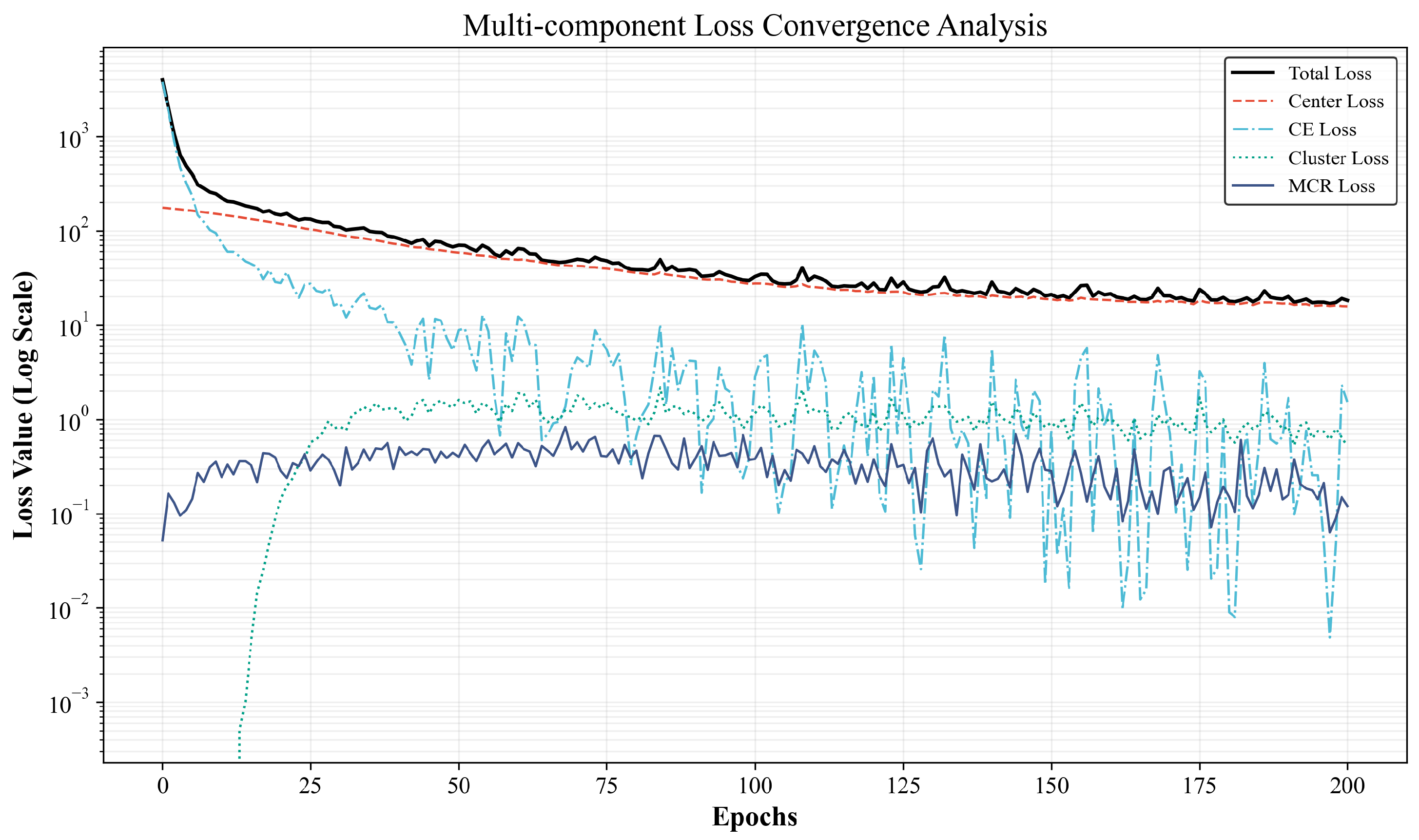
Figure 2 shows the trends in the various loss metrics during training. It can be observed that the total loss and ArcFace-CE loss decreased rapidly in the early stages of training, indicating that the model quickly learns the basic discriminative relationships between known classes. In contrast, the centrality loss and clustering loss exhibited a slower trend of change during training, suggesting that further convergence of the in-class feature distributions requires a longer optimization process. The MCR loss generally fluctuated within a narrow range, suggesting that it primarily serves as an auxiliary regularization term that constrains the feature distribution in local neighborhoods.

Overall, the multiple loss terms tended to stabilize in the later stages of training, indicating that PASM-Net achieves a relatively stable optimization process under the current experimental setup. It should be noted that the loss convergence curves are primarily used to reflect the stability of the training process; the model’s open-set recognition capability still needs to be further evaluated alongside subsequent metrics for known-class classification and unknown-class rejection.

4.2. Evaluation Criteria

The closed-set accuracy cannot fully reflect a model’s ability to reject unknown samples in an open environment. Therefore, this paper employed metrics such as the true known rate (TKR), true unknown rate (TUR), known-class precision (KP), and unknown-class precision (UP) for evaluation. Let these terms denote the number of test samples classified by the system as true known, true unknown, false known, and false unknown, respectively; the number of known samples correctly classified at the fine-grained level; and the number of unknown samples of the same class that were successfully clustered into the dominant cluster in an unsupervised setting. The mathematical expressions and physical definitions of these four core metrics are as follows:

$$TKR={\displaystyle \frac{TK}{TK+FU}},TUR={\displaystyle \frac{TU}{TU+FK}},KP={\displaystyle \frac{CK}{TK+FK}},UP={\displaystyle \frac{CU}{TU+FU}}$$

(33)

Specifically, the TKR measures the proportion of samples from the known class that are correctly classified as such; the TUR measures the proportion of samples from the unknown class that are correctly rejected; the KP measures the proportion of correctly classified samples among those predicted to belong to the known class; and the UP measures the proportion of samples that are truly unknown among those predicted to belong to the unknown class. These metrics allow for a simultaneous evaluation of the model’s ability to classify samples from the known class and its ability to reject samples from the unknown class.

4.3. Comparison of Set Recognition Benchmarks

To validate the effectiveness of PASM-Net, this paper selected S3R, SR2CNN, OpenMax, and UIOS as comparison methods. All methods were trained and tested under the same data split and input settings.

Table 2. Introduction to comparative methods.

Setting Method	Required Data	Goal
1: PASM-Net (Proposed)	Known classes	Classifying known classes and classifying unknown classes
2: S3R	Known classes	Classifying known classes and classifying unknown classes
3: SR2CNN	Known classes	Classifying known classes and classifying unknown classes
4: OpenMax	Known classes	Classifying known classes and rejecting unknown classes
5: UIOS	Known classes	Classifying known classes and rejecting unknown classes

summarizes the training data requirements and task objectives for the different methods.

Among these, S3R [20], SR2CNN [21], OpenMax [13], and UIOS [22] are state-of-the-art OSR methods. Of the methods compared here, only S3R and SR2CNN can classify unknown classes. Using the same settings as in previous work—and adopting the same settings for S3R and SR2CNN as in this paper—we compared our method with several advanced architectures to establish a comprehensive benchmark. In this paper, we constructed six scenarios with varying degrees of openness. The detailed known/unknown class assignments for all 24 drone types in each Scenario are explicitly provided in

Table 3. Known/unknown class assignments for the six open-set scenarios on the DroneRFb-Spectra dataset.

Scenario	Splitting Setting	Classes
I	known class (18)	A, B, C, D, F, K, L, M, N, O, P, Q, R
	unknown class (6)	E, G, H, I, J, W
II	known class (20)	A, B, C, D, F, G, H, K, L, M, N, O, P, Q, R, S, T, U, V, X
	unknown class (4)	E, I, J, W
III	known class (22)	A, B, C, D, F, G, H, I, K, L, M, N, O, P, Q, R, S, T, U, V, W, X
	unknown class (2)	E, J
IV	known class (23)	A, B, C, D, E, F, G, H, I, J, K, L, M, N, P, Q, R, S, T, U, V, W, X
	unknown class (1)	O
V	known class (16)	A, B, C, D, F, K, L, M, N, P, R, S, T, U, V, X
	unknown class (8)	E, G, H, I, J, O, Q, W
VI	known class (14)	A, C, D, F, K, L, M, P, R, S, T, U, V, X
	unknown class (10)	B, E, G, H, I, J, N, O, Q, W

. Scenarios I–VI differed in both the number and composition of known and unknown classes and were used to evaluate the model’s stability under different degrees of openness. The experiments were run multiple times, and the average results are reported.

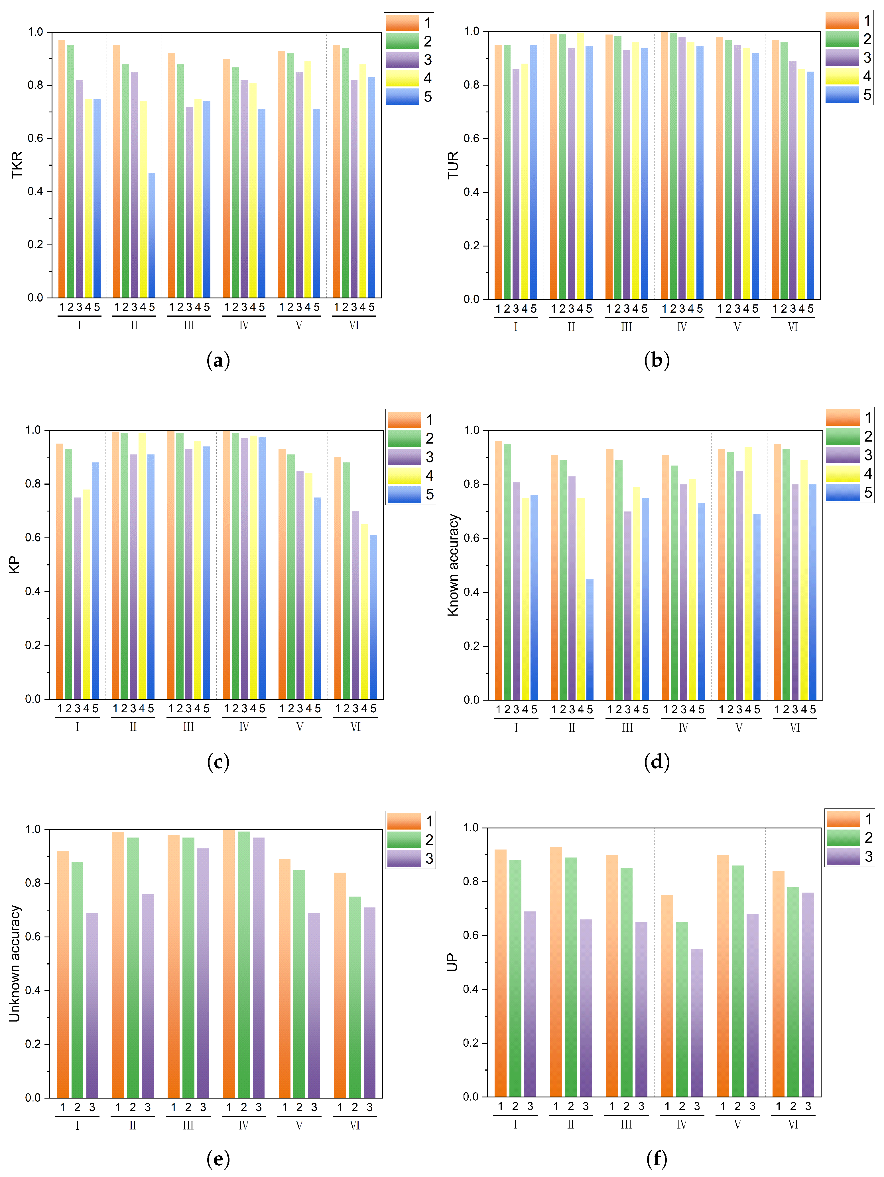
As shown in Figure 3, PASM-Net outperformed the existing methods, including S3R and SR2CNN, across various progressively open scenarios. On the TKR metric, which measures the ability to retain known classes, PASM-Net consistently maintained a score above 0.9 in all scenarios; simultaneously, on the metrics for the unknown accuracy and UP—which measure the ability to detect unknown classes—the method achieved 97.9% and 87.3%, respectively. Compared to the second-best method, PASM-Net improved the average known accuracy by 1.12% and the average unknown accuracy by 3.78%. Overall, PASM-Net achieved a strong comprehensive performance in most scenarios. Regarding the metrics for known classes, PASM-Net’s TKR and known accuracy remained high, indicating that the model can effectively retain its classification capability for known classes after introducing an unknown-sample rejection mechanism. Regarding the metrics related to unknown classes, PASM-Net’s unknown accuracy and UP also outperformed most comparison methods, suggesting that its distance-threshold decision-making can, to some extent, enhance the ability to reject unknown samples.

It should be emphasized that the TUR and unknown accuracy evaluate different stages of open-set recognition. The TUR reflects the ability to detect and reject unseen samples at the known/unknown decision stage. In contrast, the unknown accuracy and UP further characterize the fine-grained recognition performance of samples identified as unknown. Therefore, a high TUR indicates reliable unknown detection, whereas the unknown accuracy and UP reflect the subsequent discrimination capability among unknown classes.

4.4. Module Ablation Experiment

As shown in

Table 4. Ablation study of different components on the DroneRFb-Spectra dataset.

Metrics	Base	coordatt	mcr_coordatt	mcr_coordatt_Arc
TKR	0.9621	0.9528	0.9621	0.9741
TUR	0.9087	0.9296	0.9389	0.9418
KP	0.8471	0.8769	0.8923	0.9563
Known Accuracy	0.9108	0.8525	0.9030	0.9734
Unknown Accuracy	0.6953	0.6849	0.8047	0.9233
UP	0.7048	0.7781	0.8007	0.9209

, after adding CoordAtt alone, both the KP and UP improved compared to the base model, indicating that coordinate attention helps, to some extent, enhance the prediction accuracy. However, the known accuracy and unknown accuracy did not improve in tandem, suggesting that recalibration based solely on position-related features is insufficient to improve all open-set metrics consistently. This result also suggests that CoordAtt is better suited as a foundational feature-enhancement module and should work in conjunction with subsequent semantic constraints and angular metrics.

After further incorporating MCR on top of CoordAtt, the TUR, KP, unknown accuracy, and UP all improved, indicating that the local smoothing constraint based on the Laplace graph helps improve the local consistency of the known-class feature distribution and enhances the rejection performance for unknown samples. In particular, the unknown accuracy improved from 0.6849 to 0.8047, indicating that MCR positively impacts the stability of the open-set decision boundary.

Upon further integration of the ArcFace classification head, the model achieved the best results in this set of experiments across all six metrics. Specifically, the known Accuracy improved from 0.9030 to 0.9734, the unknown accuracy from 0.8047 to 0.9233, and the UP from 0.8007 to 0.9209. These results indicate that the local constraints imposed by MCR on feature distributions and the enhancement of angular separation between classes provided by ArcFace are complementary: The former helps reduce the local dispersion of features within known classes. At the same time, the latter enhances the angular separability between known classes. When combined, these approaches make the open-set threshold decision based on the cosine distance more stable.

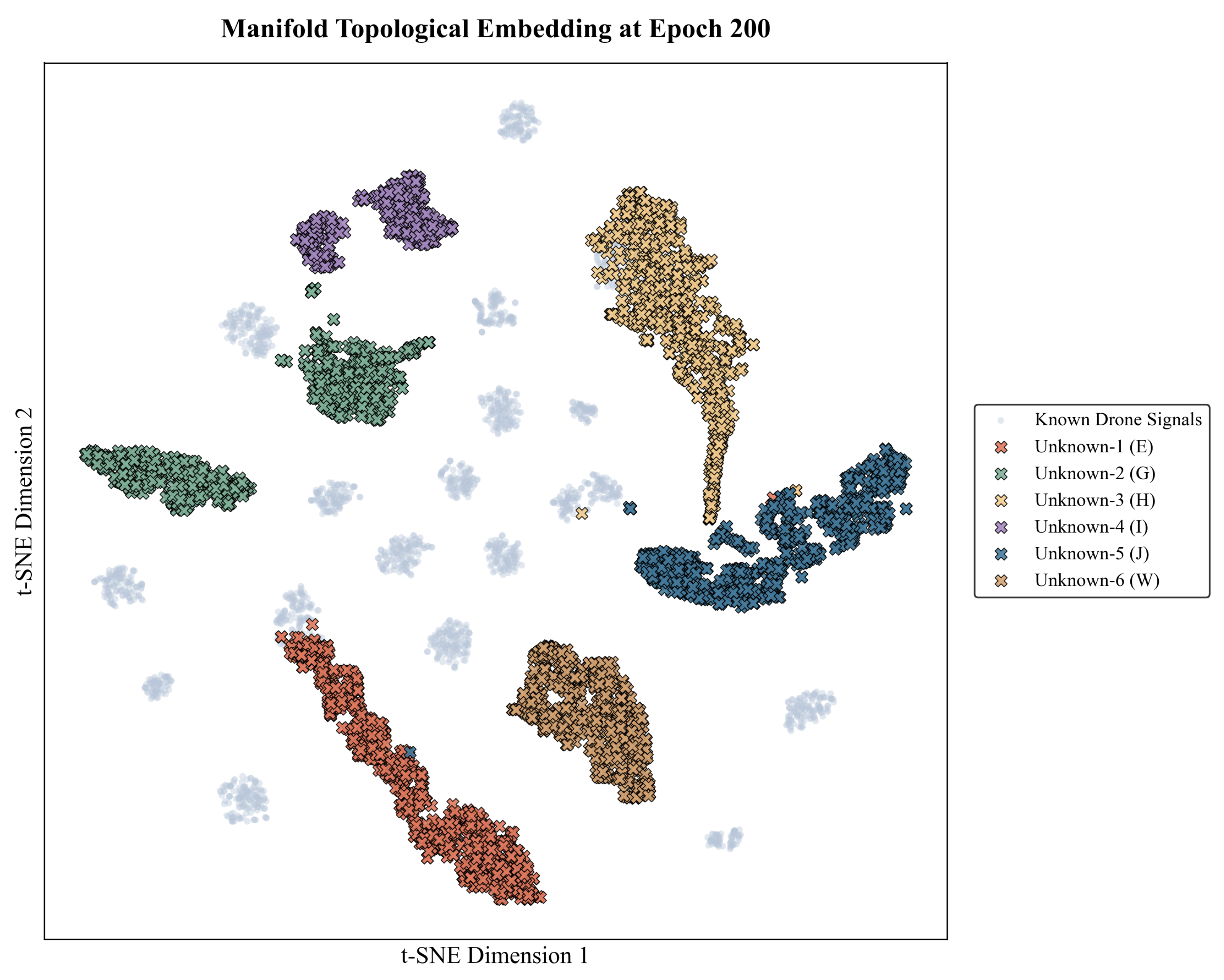
Figure 4 shows the feature visualization results for Scenario I. It can be observed that, under the full model, the distribution of known-class samples is more concentrated, and unknown samples show a more pronounced tendency to separate from the known-class clusters. These visualization results provide an intuitive illustration of the effects of MCR and ArcFace on the structure of the feature space.

4.5. Sensitivity Analysis of Loss Weights

To further investigate the influence of different loss weights on the open-set recognition performance of PASM-Net, a one-factor-at-a-time sensitivity analysis was conducted for ${\eta }_1$, ${\eta }_2$, ${\eta }_3$, and ${\eta }_4$, which correspond to the center loss, cluster loss, ArcFace-CE loss, and MCR loss, respectively. 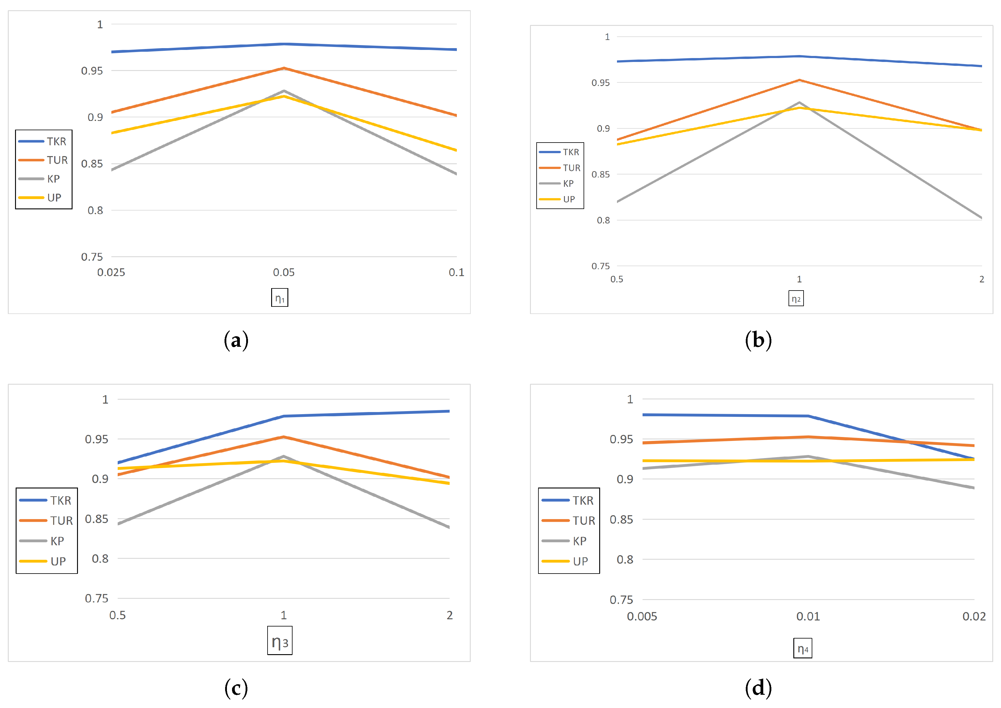Taking the default configuration $({\eta }_1,{\eta }_2,{\eta }_3,{\eta }_4)=(0.05,1.0,1.0,0.01)$ as the reference, each loss weight was independently varied while the remaining weights were kept fixed. Specifically, each weight was evaluated at approximately $0.5\times$, $1\times$, and $2\times$ its default value. The TKR, TUR, KP, and UP were used to evaluate the performance variation under different weight settings, as shown in Figure 5.

As shown in Figure 5a, increasing ${\eta }_1$ from 0.025 to its default value of 0.05 improved both the TUR and KP, whereas further increasing it to 0.1 resulted in a decrease in these metrics. This indicates that an appropriate center-loss constraint can improve intra-class compactness, while an excessively large weight does not further benefit open-set discrimination. For ${\eta }_2$, Figure 5b shows that the default value of 1.0 provided a favorable balance among the TUR, KP, and UP, whereas either reducing or excessively increasing the cluster-loss weight led to degradation in some metrics.

For the ArcFace-CE loss weight ${\eta }_3$, Figure 5c shows that the TKR generally increased as the weight became larger, indicating that stronger classification supervision benefits known-class recognition. However, when ${\eta }_3$ exceeded its default value, the TUR, KP, and UP decreased to different extents, suggesting that excessive emphasis on known-class classification may adversely affect the balance between known-class recognition and unknown-sample rejection. Regarding the MCR weight ${\eta }_4$, Figure 5d indicates that the model achieved a favorable overall performance around the default value of 0.01. A further increase in the MCR weight led to decreases in the TKR and KP, suggesting that excessive local manifold smoothing may restrict feature discriminability.

Overall, no single loss weight simultaneously maximized all evaluation metrics. The adopted default configuration provided a relatively stable trade-off between known-class recognition and unknown-sample rejection, indicating that PASM-Net exhibits a reasonable robustness to moderate variations in the loss weights.

5. Conclusions

To address challenges in identifying uncooperative UAVs in open, low-altitude electromagnetic environments—such as channel disturbances, the attenuation of spatiotemporal features, and difficulty rejecting unknown classes—this paper proposes PASM-Net. This open-set recognition network incorporates coordinate awareness and manifold continuity regularization. This method first extracts local time–frequency features across different receptive fields via multi-scale hollow convolution. It introduces a coordinate attention mechanism (CoordAtt) prior to global pooling to enhance the model’s ability to represent time- and frequency-position-related information. Subsequently, the model combines time-series and frequency-series branches to model global dependencies and introduces manifold continuity regularization (MCR) in the fused semantic space, reducing the dispersion of known-class feature distributions by constraining feature variations within local neighborhoods. During the classification and open-set decision phases, PASM-Net employs ArcFace to enhance the angular separability among known classes and rejects unknown samples based on the cosine distance between the test sample and the center of the known class. The experimental results on the DroneRFb-Spectra dataset show that PASM-Net achieved a strong overall performance in both known-class recognition and unknown-sample rejection, with an average true unknown rate (TUR) of 99.48%, an unknown accuracy of 97.9%, and an overall unknown class precision (UP) of 87.3%. The experimental results demonstrate that the proposed coordinate attention, local manifold regularization, and angular metric mechanisms can, to some extent, mitigate the performance trade-off between known-class classification and unknown-class rejection in open scenes.