Time-Gated Multi-Expert Generative Adversarial Network for Gearbox Fault Diagnosis

Abstract

In the domain of rotating machinery fault diagnosis, challenges such as multi-operating condition distribution heterogeneity and the difficulty of distinguishing fault features within multi-scale temporal signals persist. To address these issues, this paper introduces the Time-Gated Multi-Expert Generative Adversarial Network (TGME-GAN), a fault diagnosis approach that integrates a multi-expert gated conditional generative adversarial network with a clustering structure-aware feature enhancement. This method combines unsupervised K-means clustering with supervised discriminative learning. The optimal number of clusters is selected adaptively using the silhouette coefficient, and the distance vector from each sample to the cluster centers serves as a topological prior feature. A spatial–temporal joint representation matrix is then formed by concatenating PCA principal components, differential features, cumulative statistical features, and standardized change rates, which together capture both abrupt mutations and progressive degradation in fault signals. In the model, the discriminator incorporates a multi-expert gated network. Each expert learns a feature subspace corresponding to a distinct operating condition, and the gated network dynamically assigns fusion weights, allowing the discriminator to capture heterogeneous distributions across industrial conditions. The generator extracts multi-scale local patterns with a three-layer one-dimensional convolutional network and models sequential dependencies with a two-layer LSTM, producing high-quality fault samples that preserve intrinsic consistency. At the engineering level, TGME-GAN is deployed for gearbox fault diagnosis in uneven, small-sample industrial settings. In two gearbox fault experiments, this method substantially outperforms current mainstream models.

1. Introduction

Advances in data acquisition and analysis have enabled widespread application of machine learning and deep learning to fault detection in heavy-duty equipment, such as automotive transmissions and wind-turbine gearboxes. Wang et al. [1] developed a diagnostic method based on time-frequency representations and deep reinforcement learning (DRL), which demonstrated strong generalization and stability; Wei et al. [2] proposed a time-contracted interpretable DRL model that achieved excellent performance under high-noise conditions. In gearbox fault detection, commonly used deep learning methods face several challenges, including distribution heterogeneity across operating conditions, noise interference, and limited generalization capability.

Gearbox diagnostics primarily rely on vibration sensor signals and operational parameters, which are often subject to noise contamination and skew, so effective preprocessing of raw data is essential. Han et al. [3] enhanced signals by suppressing sidebands to improve feature discriminability in the frequency domain. He et al. [4] proposed a deep transfer learning method for fault diagnosis that achieved improved average recognition accuracy. For temporal modeling of industrial data, recurrent neural networks such as Long Short-Term Memory (LSTM), Gated Recurrent Units (GRU), and Bidirectional LSTM (BiLSTM) have been widely adopted. Keshun et al. [5] combined the multi-layer feature extraction of Quadratic Neural Networks (QNNs) with the sensitivity of BiLSTM to dynamic signal evolution, improving both accuracy and speed in fault diagnosis. These approaches focus mainly on discriminative modeling and largely ignore generative mechanisms, which limits their effectiveness in industrial settings with scarce fault samples and distribution heterogeneity across operating conditions.

In practical industrial scenarios, mechanical fault diagnosis often encounters data scarcity issues. Generative Adversarial Networks (GANs) partially alleviate few-shot limitations through adversarial training, and thus GAN-based models are commonly adopted for few-shot fault diagnosis. Zhou et al. [6] introduced a semi-supervised Deep Convolutional Generative Adversarial Network (DCGAN) for gear fault diagnosis that exploits unlabeled data alongside limited labeled samples to improve performance. Existing GAN-based methods for gearbox fault detection nonetheless suffer from several shortcomings: (1) Generator architectures built on fully connected networks are overly simple and cannot capture spatio-temporal correlations in vibration signals. (2) Discriminators lack adaptive modeling capacity, so they struggle to detect subtle faults in high-dimensional feature spaces. (3) The generation process rarely incorporates intrinsic structural information, producing samples that diverge from the true data distribution.

Common equipment-fault datasets, such as MCC5, frequently show the following problems: signal amplitudes vary widely with no clear temporal distinction between fault and normal segments; although local peaks appear, long-term dynamics indicative of “progressive degradation” or “sudden impact” are hard to detect. In the raw vibration signals, this long-term temporal dependency is obscured by noise and non-stationary operating conditions. Conventional approaches (for example, statistical feature extraction) address individual time points or sliding windows and therefore cannot capture causal evolution across longer time intervals, as shown in Figure 1.

The local signal and its spectrogram are shown in Figure 2. The raw vibration trace resembles random jitter and shows no clear periodicity or impulsive features. The right panel, which displays the short-time Fourier transform (STFT), exposes the latent structure in the time-varying frequency content. The transient impact induced by gear breakage modulates the high-frequency structural resonance response, with its energy typically concentrated within the natural frequency bands on the order of kHz. However, the high background noise makes it difficult to separate fault-related components from normal operation in the time domain. Methods that depend on hand-designed filters or fixed thresholds therefore risk missed detections and false alarms.

Fault modes overlap and class boundaries are indistinct. In the two-dimensional t-SNE embedding, as shown in Figure 3, red faulty and blue normal samples overlap substantially; they are nearly indistinguishable. In industrial practice, multiple fault types and frequent changes in operating conditions prevail. Signal variations across fault stages can be highly similar, and sparse or inaccurate labeling compounds the problem, substantially increasing classification difficulty. Industrial equipment typically contains multiple sensors whose measurements are highly correlated and partly redundant because they arise from the same underlying physical processes. Using all raw sensor signals to build a model increases model complexity and lowers training efficiency. Strong feature correlations can also cause the model to learn spurious associations instead of true fault mechanisms.

This paper proposes a structure-enhanced generative adversarial network (TGME-GAN), built on the GAN framework. The generator combines a convolutional neural network (CNN) and a long short-term memory (LSTM) network to capture local time-frequency patterns and long-range temporal dynamics. The discriminator employs a gated mixture-of-experts (MoE) mechanism to improve its discrimination of multimodal fault characteristics. During preprocessing, cluster-derived sequential features obtained from structural clustering of sensor data are embedded in the input representation. The overall architecture is implemented to enable coordinated multi-level interaction among these components.

The main contributions of this paper are as follows:

• From the domain perspective, GAN-driven approaches for gearbox fault diagnosis are still rarely explored in industrial manufacturing. Most existing GAN-based studies only utilize GAN for offline data augmentation and adopt a vanilla architecture composed of an MLP generator coupled with a single discriminator. The proposed TGME-GAN is one of the pioneering models that simultaneously optimizes the architectures of both the generator and discriminator under an integrated GAN framework for fault diagnosis. In terms of generator structural innovation, we discard the classic MLP generator and use a dedicated CNN-LSTM conditional generator adapted to gearbox vibration signals. As for discriminator structural innovation, the conventional single-network discriminator is substituted with a gating-controlled mixture-of-experts (MoE) discriminator composed of multiple expert subnetworks. This work pioneers the introduction of the MoE mechanism into the discriminator branch of GAN for fault diagnosis tasks.
• First, applying the mixture of experts (MoE) concept, we designed multiple independent expert networks to learn distinct feature subspaces in parallel. A gated network then dynamically fuses the experts’ outputs with softmax weighting, allowing the discriminator to capture conditional heterogeneity across multiple industrial working conditions. This approach addresses the limitation of conventional GANs, where a single discriminator enforces one shared discriminative mapping for all samples. When input feature dimensionality is high and heterogeneity is pronounced, a single discriminator struggles to capture both local working-condition features and global degradation patterns and thus lacks the needed adaptability.
• Second, we propose an end-to-end information channel that integrates clustering, feature injection, and joint training, automatically determining the optimal number of clusters based on the silhouette coefficient. The distance vectors are extracted from samples to each cluster center as topological prior features. This solves the problem in existing fault diagnosis methods where unsupervised clustering and supervised classification tasks usually operate independently and in parallel, and the inherent geometric structure of the data revealed by clustering fails to serve the discriminative learning.
• Third, this method simultaneously extracts differential features (instantaneous change rate), cumulative statistical features (gradual degradation trend), and standardized change rate (dimensional normalization) from time-series signals and combines them with clustering structural features to form a spatio-temporal joint representation matrix that captures multi-scale dynamic fault evolution. Most existing approaches use a single type of time-series feature and therefore overlook the coexistence of instantaneous mutations and gradual degradation in industrial signals.
• Finally, the design concatenates noise and conditional labels into a pseudo-sequence. A three-layer one-dimensional convolutional network then extracts local multi-scale patterns across layers. A two-layer LSTM further models sequence dependencies. Finally, a fully connected layer produces a feature vector with inherent consistency. This design allows the generator to capture both local statistical patterns and global structural information under conditional constraints. By contrast, existing generators mostly use MLP architectures that map noise directly to feature space and cannot model multi-scale local patterns effectively, making it difficult to ensure feature consistency and the statistical plausibility of generated samples.

The remainder of this paper is organized as follows. Section 2 reviews related work on gearbox fault diagnosis. Section 3 describes the methodology used in this study. Section 4 details the experimental procedures, specifies the equipment employed, and analyzes the experimental process. Section 5 provides a comprehensive summary and conclusion of the paper.

2. Related Work

2.1. Traditional Methods for Gearbox Fault Diagnosis

Gearboxes are critical mechanical transmission systems. Gearbox fault diagnosis primarily aims to assess whether equipment is operating normally, identify and predict early-stage faults, and analyze the root causes of failures. Fundamentally, gearbox fault diagnosis can be regarded as the recognition of operational states in rotating machinery [7]. In recent years, predictive maintenance has attracted growing attention because it can extend equipment life and reduce both repair time and repair frequency [8]. Florian et al. [9] pointed out that maintenance costs could account for 15% to 70% of the total production costs and proposed a practical decision support system (DSS) to reduce maintenance costs. Gearbox fault diagnosis is commonly performed using vibration signal analysis; it identifies and interprets characteristic vibration signatures produced by faults such as cracks or wear, and those signatures reveal the fault type. Time-domain analysis includes the Multiscale Time Synchronous Averaging (MTSA) method of Sharma et al., which improves signal-to-noise ratio by suppressing non-synchronous components [10]. Frequency-domain analysis, especially time-frequency transforms, can expose latent information in signals and thus aid assessment of mechanical health. Research in this area largely uses time-frequency methods such as wavelet transforms [11]. Envelope analysis is particularly sensitive to early-stage faults, including cracks and soft tooth defects. Feng et al. analyzed the amplitude envelope order spectrum to eliminate complex sideband orders present in the original signal’s order spectrum, thereby significantly simplifying and enhancing the reliability of gear characteristic frequency identification [12].

Conventional methods for gearbox fault diagnosis involve oil analysis and monitoring wear debris. As early as 2003, Peng et al. studied the correlation between vibration analysis and debris analysis and pointed out that debris analysis can determine the source of damage and the condition of the machine [13]. Cao et al. pointed out that the particles generated by the wear of mechanical moving parts can be monitored in real time through online oil-monitoring technology, thereby identifying the wear status of the components during the machine’s operation [14]. Meanwhile, prediction methods based on statistical process control and threshold-based alarming are relatively simple in implementation. Their core principle involves setting one or more alarm thresholds for key monitoring parameters (e.g., vibration severity, oil temperature, particle count). Wu et al. studied the quantitative characterization of the wear state and extracted indicators by using online wear particle images in order to achieve dynamic identification [15]. Conventional approaches to gear fault prediction include physical and empirical models. Yu et al. proposed a signal fusion model based on digital twin, which is used to accurately identify gearbox faults at the signal level [16].

The aforementioned method has several shortcomings: its feature engineering depends on manual design, it lacks sufficient capacity to handle high-dimensional and multivariate data, its diagnostic performance declines markedly when labeled samples are scarce, and it has limited ability to model and predict temporal evolution in depth.

2.2. Applications of Deep Learning in Gearbox Fault Diagnosis

Deep learning algorithms can effectively identify and extract fault-related information from complex and high-dimensional data, thereby enabling accurate fault classification. Early gearbox fault diagnosis primarily relied on signal-processing methods and shallow machine learning techniques. For example, Bordoloi et al. [17] employed support vector machine (SVM) in conjunction with signal-processing algorithms for multi-fault classification of gears. Shallow machine learning methods rely significantly on expert knowledge for feature engineering and demonstrate limited generalization capabilities when addressing non-stationary, nonlinear, and high-noise industrial data. Convolutional neural networks (CNNs) have shown outstanding performance in extracting local features, leading them to quickly emerge as the predominant technical approach for analyzing gearbox vibration signals. Xu et al. [18] proposed a novel improved multi-scale coarse-grained method with training interference to extract vibration features at different scales from the raw input signal. Ye et al. [19] proposed AKRNet, an attention-based kernel residual network and a novel convolutional neural network specifically designed for feature learning from gearbox vibration signals and experimentally validated its superiority.

As research into temporal dependencies and compound faults has deepened, models such as RNNs, LSTMs, and autoencoders (AEs) have been increasingly adopted for fault diagnosis. At the same time, attention has shifted toward multi-sensor fusion and improving model adaptability across varying operating conditions. Wang et al. [20] proposed Mix-VAEs, a multi-sensor information fusion model based on the variational autoencoder (VAE), for intelligent fault diagnosis. Kang et al. [21] proposed an Adam-optimized CNN-LSTM algorithm for fault diagnosis of gearboxes in wave energy converters. By combining CNN’s ability to process large-scale, high-dimensional, and nonlinear data with LSTM’s capacity to model temporal dependencies, this approach constitutes a common paradigm for time-series fault diagnosis.

Hybrid architectures such as Transformer and CNN-LSTM have become dominant in this field. Wang et al. [22] proposed a Deep Interpolation Convolutional Network (DICN) that has been experimentally validated for handling non-stationary signals. Zhou et al. [23] introduced an interpretable, parallel, spatial CNN-LSTM that improves decision accuracy. Because industrial equipment often operates under varying rotational speeds and load conditions that markedly change data distributions, deep learning methods are well suited to addressing these challenges. Existing deep learning methods are constrained at the data level by rare fault missed detection due to class imbalance and insufficient labeled samples, at the feature level by limited adaptability of fixed feature extraction pathways to different fault patterns, and at the model level by a lack of generative capability for effective training sample augmentation.

2.3. Diffusion Models

The diffusion models proposed by Ho et al. [24] are latent variable model simulations inspired by nonequilibrium thermodynamics learned a step-by-step denoising Markov chain to generate high-quality samples from random noise. Zhang et al. [25] proposed cross-domain fault diagnosis method on diffusion models to solve diagnostic problems in the industrial data-scarcity problem. Building a better denoising diffusion probability model (DDPM), they produced high-quality target domain fault data for data augmentation. Multi-level feature alignment mechanism is proposed: global feature distributions between source domain and real or generated target domains are aligned using maximal MD loss. Yangue et al. [26] proposed the noise conditioned anti-denoising diffusion implicit model (NCA-DDIM) for solving the problem of high-quality images with small-sample engineering by training a time-dependent discriminator with a VAE-guided mixed noise-conditioning method. The method overcomes the main problems of previous mainstream generative model such as unstable training, mode collapse, and small sample diversity but also low sampling efficiency, low likelihood estimation performance in some cases and low cross-domain generalization power.

2.4. Models for Gearbox Fault Diagnosis

Goodfellow et al. [27] introduced a generative adversarial network (GAN) in 2014, after which GANs were rapidly adopted for tasks such as image generation and speech synthesis. In 2016, Lei et al. [28] proposed an unsupervised, two-layer neural network that directly learns features from mechanical vibration signals. In 2018, Wang et al. [29] developed SDAE-GAN, a hybrid model that integrates a stacked denoising autoencoder (SDAE) with a GAN; experiments showed that this model yields higher classification accuracy than conventional diagnostic methods. As GAN technology matured in practical applications, more advanced variants emerged. Dixit et al. [30] used model-agnostic meta-learning (MAML) to initialize and update GAN parameters, enabling composite sample generation with limited training data and supporting intelligent fault diagnosis of rotating machinery such as gearboxes and bearings. Qian et al. [31] proposed a domain generalization framework based on decision intervals, which can indirectly achieve the distribution alignment between the source domain and the unseen target domain.

Early fault diagnosis contributes to enhancing equipment reliability, particularly for failure-prone devices operating under high-load conditions and in harsh environments. To address this problem, Su et al. [32] proposed a few-shot fault diagnosis method based on an improved generative adversarial network (GAN) and experimentally validated its effectiveness. Liao et al. [33] addressed data imbalance by introducing GANs as a novel data-generation technique to mitigate the challenges of limited and imbalanced data in practical engineering applications.

Qin et al. [34] proposed better WGAN-GP model (RE-CAWGAN-GP) for rolling bearing fault diagnosis problem under a small sample size. The goal was to improve fault data quality. Liu et al. [35] proposed multimodal gearbox fault detection method using parallel network Vision Transformer and BiGRU. The goal was to solve information loss in single-modal methods taking spatial and temporal features. Ma et al. [36] developed an interpretable hypergraph discriminative embedding method using feature cloud enhancement to solve health-monitoring problem of gear transmission systems under a very small sample background. Existing generation-model methods mostly treat GANs as standalone data-augmentation tools and separate generation from classification. Their single-generator architectures cannot build distinct models for different fault modes. Discriminators are used only for adversarial training and do not contribute to downstream diagnosis. Moreover, these methods insufficiently capture both local and global dependencies in time-series signals. On one hand, the separation between generation and diagnosis tasks leads to inconsistent model optimization goals. On the other hand, on the temporal level, GAN models are mostly convolutional or simple recurrent units limited by local receptive fields or gradient propagation bottlenecks and cannot represent short-term impact transient (local dependence) and long-term modulation patterns (global dependence) in vibration signals.

Targeting the two core demands of compound fault diagnosis under variable working conditions for mechanical equipment and model interpretability, multiple technical routes have gradually been established within the robust representation learning framework based on capsule networks. For instance, Huang et al. [37] proposed the robust weight-shared capsule network, which compresses parameter quantities via weight sharing and realizes single-fault recognition across working conditions relying on universal vibration features. Li et al. [38] put forward WavCapsNet; this network adopts wavelet convolution to extract physically interpretable impact features and traces back key diagnostic features reversely through a coupling matrix. Huang et al. [39] designed the deep adversarial capsule network. By introducing gradient reversal layer (GRL) adversarial learning, the network extracts domain-invariant features and decouples compound faults under unseen working conditions utilizing the multi-label learning capability of capsules. Lan et al. [40] proposed the Traceable Algorithm Unrolling Network. It unfolds the sparse coding algorithm into network layers and constructs a two-layer interpretable system featuring prior physical mechanism embedding and spectrum verification. These four models advance the research on representation learning for fault diagnosis from four distinct dimensions: lightweight generalization, domain-adversarial compound fault decoupling, time-frequency feature interpretability, and traceability of signal physical mechanisms.

3. Methodology

3.1. Data Sampling and Integrity Verification

The raw data derive from a gearbox monitoring system. The specific operational variables and sensor configurations differ between datasets and are detailed in Section 4.1. Specific sampling and splitting schemes for data sets are described in Section 4.1. For MCC5, 50,000 data sets are sampled from candidate pool and split into training sets and test sets. For GFD, all 3921, windowed segments are retained and split into training sets and test sets after sliding windows segments are stratified by fault labels to preserve the sampled class proportion.

The hybrid deep generative framework proposed in this paper (TGME-GAN) applies to gear fault diagnosis and related domains. It combines multi-scale sequence feature enhancement, feature clustering and dimensionality reduction, and the expert hybrid mechanism (MoE). This architecture tackles practical challenges in industrial equipment monitoring, such as complex multi-scale temporal patterns, distribution heterogeneity across operating conditions, and limited labeled samples. The framework comprises five steps: (1) sampling and integrity validation of raw data; (2) extraction of differential features, cumulative statistical features and standardized change rates from the original sensor data for sequence enhancement; (3) reduction of the feature dimension through PCA dimensionality reduction and encoding of the sample distribution structure by using K-means clustering labels and centroid distances; (4) construction of a CNN-LSTM hybrid generator—composed of convolutional neural networks (CNNs) and long short-term memory (LSTM) networks—and an MoE-based discriminator that leverages the mixture-of-experts mechanism; and (5) the design of a loss function that jointly addresses multiple optimization objectives and adoption of an adaptive optimization strategy to regulate training. Figure 4 provides an overview of the proposed methodology.

3.2. Multi-Scale Sequential Feature Learning

To capture the gradual degradation of equipment performance, four operational parameters from the original data are chosen as base features: ${\mathbf{x}}_{\mathrm{base}}={[s,t,v_{\mathrm{mx}},v_{\mathrm{my}}]}^{\top }$. Here, s denotes rotational speed, t represents torque, and $v_{\mathrm{mx}}$ and $v_{\mathrm{my}}$ indicate vibration magnitudes along the two dominant orthogonal axes. Based on these four variables, four categories of temporal features are constructed as follows:

For first-order differences, the change between consecutive time steps is computed as $\Delta {\mathbf{x}}_t={\mathbf{x}}_{\mathrm{base},t}-{\mathbf{x}}_{\mathrm{base},t-1},\mathrm{with}\Delta {\mathbf{x}}_1=0$ (since no prior value exists for the first time step).

This is implemented using np.diff in the code, with the initial position padded with zeros. For the cumulative sum and cumulative mean, the definitions are given as follows:

$$S_t={\displaystyle \sum _{i=1}^t}{\mathbf{x}}_{\mathrm{base},i},{\overline{\mathbf{x}}}_t={\displaystyle \frac{S_t}{t}}.$$

For normalized dynamic features, each base feature is the first z-score normalized by subtracting the global mean and dividing by the standard deviation, with a small constant added to the denominator to avoid division by zero. Then the first-order difference of the normalized sequence is computed.

$${\tilde{\mathbf{x}}}_t={\displaystyle \frac{{\mathbf{x}}_{\mathrm{base},t}-\mu }{\sigma +{10}^{-8}}},\Delta {\tilde{\mathbf{x}}}_t={\tilde{\mathbf{x}}}_t-{\tilde{\mathbf{x}}}_{t-1}.$$

The term “pseudo-sequence” refers to temporal features constructed from sequential data points, which are flattened and concatenated with spatial features. Specifically, given base features ${\mathit{x}}_{\mathrm{base}}\in {\mathbb{R}}^{T\times 4}$, we construct

$${\mathit{X}}_{\mathrm{temporal}}=\left[\Delta \mathit{X},\mathrm{CumSum}\left(\mathit{X}\right),\mathrm{CumMean}\left(\mathit{X}\right),\Delta {\mathit{X}}_{\mathrm{norm}}\right]\in {\mathbb{R}}^{T\times 16},$$

which captures instantaneous mutations, gradual accumulation, and dimensionless degradation rates. After construction, the values of the last time step are extracted and flattened to a vector in ${\mathbb{R}}^{16}$ per sample. Based on the tribological degradation mechanism of gearboxes, this section outlines three types of core time-series features tailored to diverse fault evolution laws: first-order difference features capture early transient fault impulse signals induced by cracks, sudden load variations and other anomalies; cumulative statistical features characterize the long-term gradual degradation trend stemming from gear abrasion and material loss; dynamic Z-score-normalized features establish a working-condition-independent dimensionless degradation rate indicators, which effectively improve the cross-working-condition generalization performance of the model. Coordinated with one another, the three categories of features can comprehensively cover the full-dimensional degradation process of gearboxes, ranging from the initiation of abrupt faults to the progressive wear evolution. In addition, mainstream time-series analysis approaches including wavelet packet transform, Hilbert–Huang transform (HHT) and empirical mode decomposition (EMD) are discarded in this section. The reasons are as follows: parameter tuning for these methods heavily relies on domain expertise; their computational overhead is substantial when processing high-frequency industrial data; furthermore, their feature decomposition logic fails to align with the actual physical degradation mechanism of gearboxes, leading to unsatisfactory generalization and adaptability.

The feature mean $\mu$ and standard deviation $\sigma$, together with each original feature and its three derived features (first-order difference, cumulative sum, and cumulative mean), form the complete feature set. These derived features are concatenated with the original features, enhancing the model’s ability to capture critical data characteristics.

3.3. Dimensionality Reduction and Clustering-Guided Structural Embedding

Existing studies fail to integrate clustering information into the generative pipeline of GANs. In this paper, cluster labels and centroid distances are adopted as structural priors to constrain both the generator and discriminator. By extending the loss function of conditional GANs, the topological distribution of generated samples is restricted, which alleviates mode collapse. Compared with alternatives such as autoencoders and graph manifold embeddings, K-means delivers superior computational efficiency, interpretability and generalization capability. To reduce the high correlation among features and avoid redundancy, features satisfying $|{\rho }_{ij}| >0.9$ are eliminated (retaining only one feature from each such highly correlated pair). Principal component analysis (PCA) is subsequently applied to the remaining features. Let the standardized feature matrix be denoted as $\mathbf{X}\in {\mathbb{R}}^{N\times d}$. The PCA transformation is then computed as follows:

$$\mathbf{Z}=\mathbf{X}\mathbf{W},\mathbf{W}\in {\mathbb{R}}^{d\times k},$$

where $k=min(d,10)$. The optimal number of principal components $k^{*}$ is selected as

$$k^{*}=min\left\{k:{\displaystyle \frac{{\sum }_{i=1}^k{\lambda }_i}{{\sum }_{i=1}^d{\lambda }_i}}\ge 0.95\right\},k^{*}\ge 2,$$

where ${\lambda }_i$ is the eigenvalue of the covariance matrix.

Next, k-means clustering is applied to the principal component scores to identify latent distributional structure in the feature space. While the silhouette coefficient (0.27 at $K=2$) indicates relatively weak separation, metadata validation (ANOVA against ground-truth speed and load) reveals that clusters primarily separate along the speed dimension ($F=9.91\times {10}^6$, $p<0.001$) rather than the load condition (F = 0.31, p = 0.58). These clusters therefore reflect data-driven geometric partitions aligned with the dominant PCA variance axis, rather than pre-defined physical operating regimes. Nevertheless, the distance-to-centroid features encode each sample’s topological position in the latent space, providing the discriminator with distributional priors that enhance feature discrimination. The number of clusters is chosen by maximizing the silhouette coefficient over the range $K\in [2,min(10,{\displaystyle \frac{N}{10}})]$, ensuring the clustering is neither overly fragmented nor under-discriminative. Each sample is then augmented with the following information:

Clustering label: $c_i\in \{0,1,\dots ,K-1\}$; Distances to all cluster centroids: $d_i^{\left(k\right)}={\parallel {\mathbf{z}}_i-{\mathsf{\mu }}_k\parallel }_2$; Scores of the first $k^{*}$ principal components: ${\mathbf{z}}_{i,1},\dots ,{\mathbf{z}}_{i,k^{*}}$.

This yields a structurally enhanced feature vector ${\mathbf{x}}^{\mathrm{enh}}\in {\mathbb{R}}^{d_{\mathrm{total}}}$, where $d_{\mathrm{total}}=d_{\mathrm{clean}}+K+k^{*}+16$. The enhanced feature vector has 36 dimensions in total and is composed of five feature groups: (1) Original features after correlation filtering (9 dimensions: rotational speed, torque, six vibration signals and mechanical load); (2) Cluster label (1 dimension, with the number of clusters set to 2); (3) Euclidean distances from samples to each cluster centroid (2 dimensions); (4) PCA principal components that retain 95% cumulative variance (8 dimensions); (5) Multi-scale temporal features (16 dimensions), generated by applying four transformation operations to four basic physical features. Summing the dimensions of all five groups yields a total feature dimension of 36.

3.4. Deep Generative Architecture

Aiming at the dual characteristics of gearbox signals, i.e., local high-frequency impulses and long-term temporal degradation trends, this paper adopts a hybrid CNN-LSTM generator. Compared with Transformer, MLP, pure CNN and pure LSTM architectures, the proposed hybrid structure can simultaneously extract local fault features and model temporal evolution patterns, outperforming all other single-network alternatives. We designed a deep generative model to synthesize richer fault diagnosis features. The generator G maps a latent vector $\mathbf{z}\sim \mathcal{N}(0,{\mathbf{I}}_{256})$ and a conditional label $\mathbf{y}$ to a synthetic augmented feature:

$$\widehat{\mathbf{x}}=G(\mathbf{z},\mathbf{y}).$$

Tensor shape specifications: Let B represent the batch size, with a fixed value of 64. (1) Generator input: Random noise and category labels are combined together. After concatenation, the overall dimension is adjusted through the unsqueeze function to adapt to the network input requirements. (2) Generator output: The network outputs enhanced feature vectors with a total of 36 dimensions for each sample. (3) Discriminator input: Raw feature vectors are concatenated with corresponding labels as the input data of the discriminator. (4) Discriminator output: The discriminator contains two independent output branches, namely the adversarial discrimination branch and the fault classification branch, both of which finally output one-dimensional results for each sample. For conditional label encoding, labels are encoded in binary form: 0 corresponds to healthy operating conditions, and 1 corresponds to fault conditions. Labels are directly spliced with noise data or feature data. In the training process, the generated simulated samples keep consistent with the actual label distribution of the training set so as to achieve category-conditional fault sample generation. Its architecture comprises 1D CNN: The model uses three Conv1d layers with channel counts increasing from 32 to 64 and then to 128. Each convolution uses a kernel size of 3 and padding to preserve sequence length. After each Conv1d, a BatchNorm layer and a LeakyReLU activation (negative slope = 0.2) are applied, followed by MaxPool1d with stride 2 for downsampling.

The one-dimensional convolutional long short-term memory network (1D CNN-LSTM) embedded within the generator is not designed to model the physical temporal dynamics of noisy inputs; instead, it serves as a hierarchical feature synthesis module. Its three convolutional layers are configured with channel counts of 32, 64, and 128 in sequence. Relying on learnable weight sharing and local connections, the module progressively converts unstructured noise into multi-scale structured feature maps. This design philosophy aligns with the mechanism adopted by DCGAN, which reshapes noise and subsequently employs two-dimensional convolutions for image generation. The LSTM component further exploits correlations among features at diverse scales to ensure the intrinsic consistency of the output feature vectors. Compared with generators built solely upon multilayer perceptrons (MLPs), the proposed architecture incorporates structured inductive bias, and the effectiveness of this method has been validated through subsequent experiments.

LSTM: The CNN output is interpreted as a time series and fed into a two-layer LSTM. Each layer has 64 hidden units. We apply a dropout rate of 0.5 between layers to mitigate overfitting.

Fully connected layers: Two linear layers ($64\to 128\to D_{\mathrm{total}}$) are applied, with BatchNorm and LeakyReLU placed between them. The final output dimension matches that of the constructed augmented feature vector.

The discriminator D consists of 12 expert subnetworks and adopts a conventional gated mixture-of-experts (MoE) architecture. Given the input $[\mathbf{x},\mathbf{y}]$, the concatenation of the feature vector $\mathbf{x}$ and the label $\mathbf{y}$, the gating network computes the expert weights as $\mathbf{g}=\mathrm{softmax}\left({\mathrm{MLP}}_{\mathrm{gate}}\left([\mathbf{x},\mathbf{y}]\right)\right)\in {\mathbb{R}}^M$, where $M=12$. The choice of M = 12 is motivated by both empirical and structural considerations. The gearbox data contains multiple latent sub-patterns arising from variations in speed, load, and degradation stage; the specific contribution of each factor is not assumed to be identical. With 12 experts, each expert can specialize in a distinct sub-pattern while the gating network efficiently routes samples. Beyond 12, additional experts lead to routing redundancy and decreased per-expert utilization. Pairwise similarity analysis of expert outputs confirms that no expert pair exhibits similarity > 0.7, indicating that all 12 experts learn complementary rather than redundant representations. Each expert $E_m$ is implemented as a three-layer MLP. The fused representation is then obtained as

$$\mathbf{h}={\displaystyle \sum _{m=1}^M}{g}_m·E_m\left([\mathbf{x},\mathbf{y}]\right),$$

and is split into two branches:

Adversarial head $D_{\mathrm{adv}}={\mathbf{w}}_a^{\top }\mathbf{h}+b_a$;

Classification head $D_{\mathrm{cls}}=\sigma \left({\mathrm{MLP}}_{\mathrm{cls}}\left(\mathbf{h}\right)\right)$.

The current classification head uses a single sigmoid output for binary detection. It can be directly extended to multi-class by replacing it with a softmax layer of $C+1$ neurons.

3.5. Optimization

We adopt a multi-objective joint training strategy in which the generator and discriminator are updated alternately on a per-batch basis. The training optimizes two primary loss terms. Let ${\mathcal{L}}_{\mathrm{adv}}$ denote the binary cross-entropy loss with logits, used to discriminate real from generated samples. Let ${\mathcal{L}}_{\mathrm{cls}}$ denote the standard binary cross-entropy loss, used to supervise the model’s prediction of the “normal/fault” label.

Discriminator loss ${\mathcal{L}}_{\mathrm{D}}$:

$$\begin{array}{cc}\hfill {\mathcal{L}}_{\mathrm{D}}=& {\mathcal{L}}_{\mathrm{adv}}\left({\mathrm{D}}_{\mathrm{adv}}({\mathbf{x}}_{\mathrm{real}},\mathbf{y}),1\right)\hfill \\ & +{\mathcal{L}}_{\mathrm{adv}}\left({\mathrm{D}}_{\mathrm{adv}}(\mathrm{G}(\mathbf{z},\mathbf{y}),\mathbf{y}),0\right)\hfill \\ & +{\lambda }_{\mathrm{cls}}·{\mathcal{L}}_{\mathrm{cls}}\left({\mathrm{D}}_{\mathrm{cls}}({\mathbf{x}}_{\mathrm{real}},\mathbf{y}),\mathbf{y}\right)\hfill \end{array},$$

where ${\lambda }_{\mathrm{cls}}=2.5\times {10}^{-6}$.

Choosing an extremely small ${\lambda }_{\mathrm{cls}}$ is a deliberate design. Our dual-task discriminator computes adversarial loss via BCEWithLogitsLoss. Conventional larger ${\lambda }_{\mathrm{cls}}$ values would let classification gradients control discriminator updates, leading to classification overfitting, impaired adversarial discrimination, and generator mode collapse. Set to $2.5\times {10}^{-6}$, the classification loss only accounts for around ${10}^{-6}$ of total loss. This configuration delivers steady gradients to the classification head whilst preserving stable adversarial training, following the auxiliary task weighting rule for multi-task GANs.

Generator loss ${\mathcal{L}}_{\mathrm{G}}$:

$${\mathcal{L}}_{\mathrm{G}}={\mathcal{L}}_{\mathrm{adv}}\left({\mathrm{D}}_{\mathrm{adv}}\left(\mathrm{G}\left(\mathbf{z},\mathbf{y}\right),\mathbf{y}\right),1\right)+{\lambda }_{\mathrm{cond}}·{\mathcal{L}}_{\mathrm{cls}}\left({\mathrm{D}}_{\mathrm{cls}}\left(\mathrm{G}\left(\mathbf{z},\mathbf{y}\right),\mathbf{y}\right),\mathbf{y}\right),$$

where ${\lambda }_{\mathrm{cond}}=0.4$.

All networks were trained with gradient clipping $(\parallel \nabla \parallel \le 0.5)$ and optimized using the Adam optimizer (learning rate = 0.001, ${\beta }_1=0.5$, ${\beta }_2=0.999$). The learning rate was reduced adaptively by ReduceLROnPlateau (patience = 5) based on validation-set AUC. Training proceeded for 200 epochs, with model evaluation every 10 epochs. This evaluation schedule produced 21 checkpoints (at epochs 0, 10, 20, …, 190, 200). For brevity, the x-axis of subsequent AUC curve plots used checkpoint indices (1–21) to represent training progress. Weights of linear and convolutional layers were initialized orthogonally, and all biases were set to zero. For the synthetic sample integration strategy in TGME-GAN, synthetic samples are implicitly utilized through adversarial learning rather than explicit data augmentation. The discriminator serves dual purposes: (1) during GAN training, it is jointly trained on real and synthetic samples through adversarial and classification losses, learning robust feature representations, and (2) during inference, the trained discriminator is applied directly to real test samples for fault classification. This unified approach eliminates the generation-diagnosis separation present in conventional two-stage GAN methods, where synthetic samples are generated offline and used to augment the training set before training a separate classifier.

We evaluated the fidelity of generated samples using the following metrics. All metrics were computed in the standardized enhanced feature space (Section 3.3), with real samples from the test set and generated samples produced by the trained generator under matching class labels.

We used unbiased estimator of ${\mathrm{MMD}}^2$ with a multi-scale Gaussian kernel. The bandwidth was calibrated via the median heuristic on the pooled sample set and evaluated at five scales $\{0.25,0.5,1.0,2.0,4.0\}\times {\gamma }_0$, where ${\gamma }_0=1/\left(2d_{\mathrm{med}}^2\right)$:

$${\mathrm{MMD}}^2={\displaystyle \frac{1}{5}}\sum _s\left[{\displaystyle \frac{{\sum }_{i\ne j}{k}_{s{\gamma }_0}(x_i,x_j)}{n(n-1)}}+{\displaystyle \frac{{\sum }_{i\ne j}{k}_{s{\gamma }_0}({\widehat{x}}_i,{\widehat{x}}_j)}{m(m-1)}}-{\displaystyle \frac{2{\sum }_{i,j}{k}_{s{\gamma }_0}(x_i,{\widehat{x}}_j)}{nm}}\right]$$

• FID-style Distance.

We adapted the Fréchet distance to tabular features by computing it in the discriminator’s MoE gating layer output space (128-dimensional; Section 3.4), which provided a discriminatively informed embedding analogous to inception features in the original FID:

$$\mathrm{FID}= \parallel {\mu }_r-{\mu }_g{\parallel }^2+Tr\left({\sum }_r+{\sum }_g-2{\left({\sum }_r{\sum }_g\right)}^{1/2}\right)$$

where $\mu ,\sum$ denotes the means and covariances in the gating-layer space.

• Wasserstein Distance and Variance Ratio.

The per-dimension 1-Wasserstein distance $W_d={\int }_0^1|F_{r,d}^{-1}\left(t\right)-F_{g,d}^{-1}\left(t\right)|dt$ is averaged as $\overline{W}={\displaystyle \frac{1}{D}}{\sum }_d{W}_d$. The variance ratio $\mathrm{VR}={\displaystyle \frac{1}{D}}{\sum }_d{\sigma }_{g,d}^2/{\sigma }_{r,d}^2$ measures diversity preservation.

• Class-Conditional Coverage.

For each class c, the threshold ${\tau }_c$ is the 95th percentile of the k-th nearest-neighbor distances ($k=min(6,|{\mathcal{R}}_c\left|\right)$) within real samples of that class. Coverage is the fraction of real samples whose distance to the nearest generated sample of the same class is below ${\tau }_c$:

$${\mathrm{Coverage}}_c={\displaystyle \frac{1}{|{\mathcal{R}}_c|}}\sum _{x\in {\mathcal{R}}_c}\mathbb{1}\left[\underset{\widehat{x}\in {\mathcal{G}}_c}{min}{\parallel x-\widehat{x}\parallel }_2<{\tau }_c\right]$$

• Downstream Classification.

A classifier trained on 1000 generated samples (500 per class) and evaluated on the real test set measures the practical utility of synthetic data.

4. Experiments

4.1. Experimental Setting

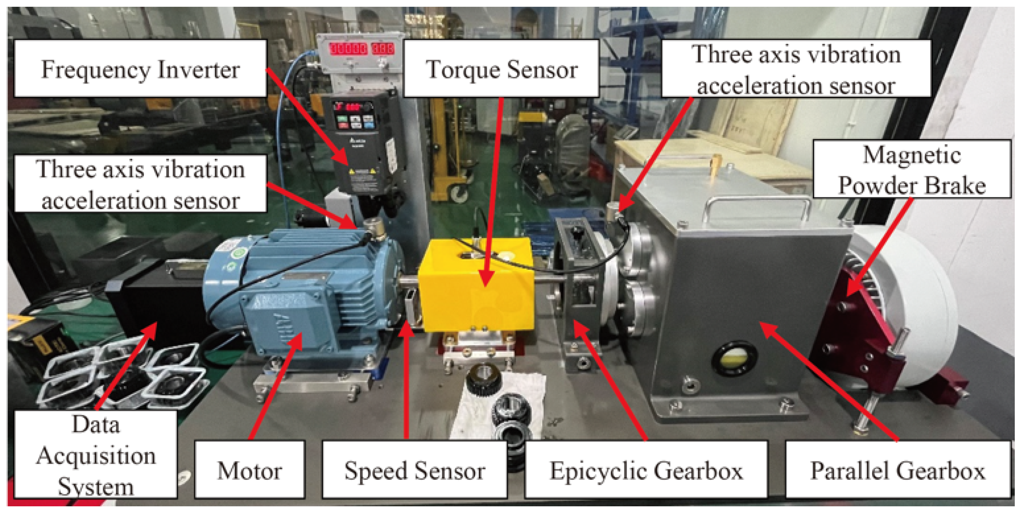
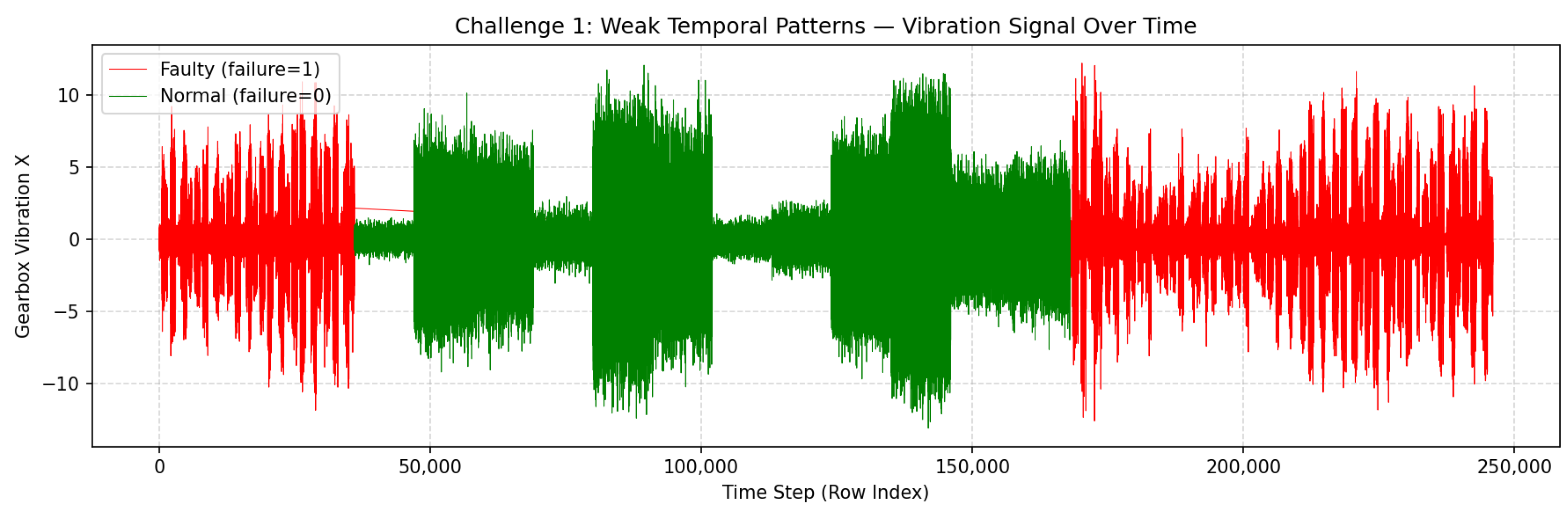
Datasets: We conducted our study on a benchmark dataset collected by the Department of Automation at Tsinghua University [41]. The dataset was MCC5. The experimental equipment is shown in Figure 5. This dataset is well suited for evaluating the robustness of fault diagnosis algorithms across varying operating conditions. Data were acquired on an experimental platform consisting of a three-phase asynchronous motor, two triaxial vibration accelerometers (model TES001V) mounted on the motor drive end and the gearbox intermediate shaft to record triaxial vibration acceleration, a torque sensor to measure gearbox input-shaft torque, and an optical encoder to capture key-phase and rotational-speed signals from the motor output shaft. The platform also included a two-stage parallel gearbox and a magnetic-powder brake to apply controllable torque loads. A total of 240 experimental files were produced, covering 24 steady-state and 48 transient-state operating-condition combinations. There were 12 normal status files, totaling 9,215,988 lines (accounting for approximately 5.00%), and 228 faulty status files, with a total of 175,103,772 lines (accounting for approximately 95.00%). To obtain a computationally feasible working dataset, we conducted stratified random sampling, extracting 11,000 lines from each normal file and 500 lines from each faulty file. Eventually, we obtained a candidate pool containing 246,000 records. To maintain consistency with the small-sample industrial setting and ensure computational efficiency, 50,000 records were then randomly sampled from this pool for subsequent experiments, preserving the class distribution of the constructed candidate pool. Each dataset was sampled at 12.8 kHz and contained the speed signal, torque signal, triaxial vibration signals (x, y, z) from the motor, and triaxial vibration signals (x, y, z) from the gearbox intermediate shaft. For variable-speed tests, the load was set to 10 Nm or 20 Nm; for variable-load tests, the rotational speed was fixed at 1000, 2000, or 3000 rpm. The dataset included signals for seven gear-fault conditions and one healthy condition.

This paper introduces a gearbox fault diagnosis dataset [42] to validate the effectiveness and robustness of the proposed method. The GFD dataset contains four-channel vibration records of both broken teeth and normal conditions. At the raw signal level, the dataset itself consists of a balanced total of 2,021,119 rows. After sliding-window segmentation (window size = 1024, stride = 512), the raw GFD recordings yielded a total of 3921 windowed segments. Given this limited sample size, all available segments were retained for experimentation rather than subsampling. A stratified 80/20 split was then applied, resulting in 3137 training samples and 784 test samples. This full-utilization strategy ensured that no diagnostic information was discarded from an already small-scale benchmark. Data were acquired from four vibration sensors mounted in orthogonal directions while the load was varied from 0% to 90%. The dataset primarily covered normal conditions and tooth damage faults. These files corresponded to varying load levels, starting from 0% and incrementing in steps of 10% up to 90%.

Baselines: In order to conduct a comprehensive experimental comparison, we divided the selected models into two groups. Group 1 comprised traditional machine learning methods: XGBoost, Random Forest, and SVM. Group 2 included time-series modeling approaches, primarily LSTM, GAN, and CNN. Conventional fault diagnosis relies largely on the methods in Group 1, which typically depend on steady-state assumptions or handcrafted features and therefore struggle to accommodate mode drift under changing operating conditions. To mitigate this limitation, we also included representative methods from fault diagnosis and open-set classification as additional baselines. Support vector machines (SVMs) nonlinearly map input vectors into a high-dimensional feature space and construct a linear decision surface to ensure high generalization capability [43]. Random Forest (RF) is employed as a data fusion tool to integrate deep feature representations, thereby improving the performance of gearbox fault diagnosis [44]. XGBoost is a novel sparsity-aware algorithm for sparse data, which optimizes the fault discrimination boundary through gradient boosting [45].

Common time-series models mainly include LSTM, GAN, and CNN. Zhu et al. employed CNN-Transformer to extract local features and model the long-term dependencies within the sequence [46]. Guo et al. proposed an improved adversarial learning method to generate fault features in order to address the problem of imbalance in fault categories [47]. 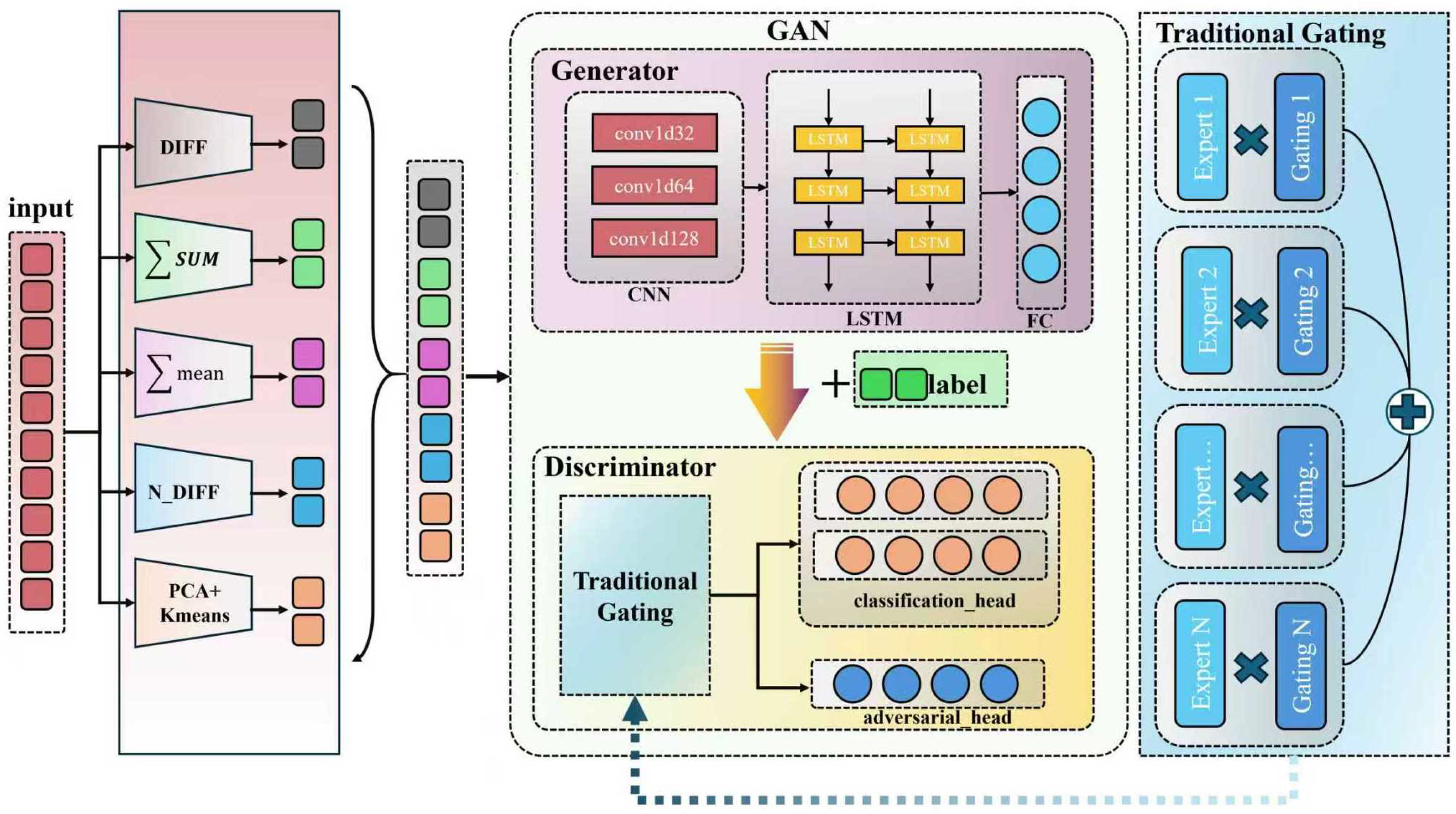In addition, the hybrid CNN-LSTM architecture effectively integrates local and global temporal features [48]. In gearbox fault diagnosis, this paper employs four methods (deep generative modeling, a sequential modeling architecture, clustering-guided feature learning, and multi-expert fusion) to ensure effective feature enhancement and classification.

Evaluation Metrics: Considering the inherent characteristics of industrial fault diagnosis, we adopted AUC and ACC as the primary evaluation metrics to comprehensively assess model performance. These metrics are widely adopted in the fault diagnosis literature [49]. AUC and ACC were used as the primary quantitative evaluation metrics. KDE was used as a visualization tool to compare the distributions of selected real and generated features.

Experimental Settings: We set the five core parameters as hyperparameters and conducted an analysis on each one. These parameters were: latent space dimensionality, number of expert networks, discriminator classification loss weight, generator classification loss weight, and optimizer learning rate. Each parameter was varied in the corresponding fault classification and recognition tasks. We then analyzed the specific effects of these hyperparameters on the overall model.

The data preparation was different between the two benchmarks because of scale differences. For MCC5, 50,000 records were sampled randomly (seed = 42) and split into 40,000 training and 10,000 test samples. For GFD, all 3921 windowed segments were split stratified 80/20 (3137 training and 784 test). Despite differences in absolute samples, all models were trained and tested within the same data set for fair intra-dataset comparison. Cross-dataset performance trends continue to be valid since they reflect method robustness across different data regimes. Stratified sampling was used to maintain the proportion of each category within each dataset. This work used a feature-engineering-based representation enhancement scheme, which concretely comprised differential features, cumulative statistical features (cumulative sum and cumulative mean), standardized rate-of-change features, and data structural features extracted via PCA–K-means cluster analysis (including cluster labels, distances to each cluster centroid, and principal components). The aforementioned augmentation strategies enriched the feature representations utilized by the model and were verified via the ablation experiments presented below. The model in this study was implemented with the following hyperparameter configurations: batch size = 64, maximum training epochs = 200, latent space dimension = 256, number of expert networks = 12, gradient clipping threshold = 0.5, and with each individual run using a fixed random seed. The ablation study and the detailed validation in Section 4.6 were a representative run with seed = 42, whereas the comparative results in

Table 1. Model Comparison (Across Different Datasets).

Model	MCC5		Gearbox Fault Diagnosis
	Accuracy	AUC	Accuracy	AUC
RandomForest	0.6294 ± 0.0041	0.6653 ± 0.0047	0.6571 ± 0.0042	0.7184 ± 0.0039
SVM	0.6341 ± 0.0065	0.6912 ± 0.0053	0.6642 ± 0.0044	0.7106 ± 0.0048
MHTA-DDPM	0.7890 ± 0.0437	0.9041 ± 0.0209	0.8785 ± 0.0097	0.9240 ± 0.0047
GAN	0.6415 ± 0.0131	0.6922 ± 0.0346	0.6718 ± 0.0144	0.6953 ± 0.0253
CNN-LSTM	0.7374 ± 0.0032	0.7721 ± 0.0084	0.7865 ± 0.0025	0.7705 ± 0.0131
XGBoost	0.6477 ± 0.0341	0.6911 ± 0.0336	0.6842 ± 0.0335	0.7231 ± 0.0304
WGAN-GP	0.7718 ± 0.0040	0.8878 ± 0.0034	0.7918 ± 0.0030	0.8874 ± 0.0028
RF+LSTM	0.7165 ± 0.0031	0.7613 ± 0.0042	0.7154 ± 0.0029	0.7726 ± 0.0037
RF-GRNN	0.7109 ± 0.0124	0.7504 ± 0.0109	0.7215 ± 0.0153	0.7917 ± 0.0161
SWT-VGG-LSTM	0.6916 ± 0.0258	0.7375 ± 0.0245	0.6473 ± 0.0311	0.7620 ± 0.0265
CNN GTFE_Net	0.7195 ± 0.0031	0.7661 ± 0.0023	0.7432 ± 0.0075	0.7873 ± 0.0058
SECN	0.7784 ± 0.0017	0.8398 ± 0.0024	0.7915 ± 0.0011	0.8830 ± 0.0031
GRU-AM-TL	0.7815 ± 0.0264	0.8523 ± 0.0301	0.8123 ± 0.0254	0.8903 ± 0.0213
CNN MT-ConvFormer	0.7169 ± 0.0012	0.7639 ± 0.0007	0.7169 ± 0.0012	0.7626 ± 0.0257
TGME-GAN	0.8614 ± 0.0114	0.9128 ± 0.0132	0.9022 ± 0.0151	0.9611 ± 0.0147

were aggregated over multiple predefined seeds. Both the generator and discriminator utilized the Adam optimizer with an initial learning rate of 0.001. For the quality verification of generated data, 500 samples were generated for each category (healthy and faulty states), yielding a total of 1000 synthetic samples. All experiments were conducted on a hardware platform equipped with an NVIDIA GeForce RTX 3080 10 GB GPU (NVIDIA Corporation, Santa Clara, CA, USA), an Intel Core i5-14400F CPU (Intel Corporation, Santa Clara, CA, USA), and 32 GB RAM (Corsair, Fremont, CA, USA). The runtime for one complete training procedure was approximately 10 h.

To ensure rigorous evaluation without data leakage, we strictly adhered to the following protocol: (1) The dataset was first split into training (80%) and test (20%) sets using stratified sampling. (2) All preprocessing steps, including standardization, correlation-based feature selection, PCA dimensionality reduction, and K-means clustering, were fitted exclusively on the training set. (3) The fitted transformations were applied to the test set without refitting. (4) No information from the test set influenced any aspect of feature engineering or model training. This protocol prevented transductive leakage and ensured that the reported metrics reflected true generalization performance.

4.2. Performance Analysis

Comparative experiments were conducted on the gearbox fault diagnosis dataset and the MCC5 dataset to validate the effectiveness of the proposed model. In these comparative experiments, ACC and AUC were adopted as the primary evaluation metrics to compare TGME-GAN with various machine learning and deep learning methods. As shown in Table 1, the experimental results indicate that the proposed TGME-GAN model outperforms the baseline model on both datasets.

Since these models were developed for different applications, we applied the following modifications to ensure compatibility with GFD and MCC5 data: MHTA-DDPM [50] time-frequency fusion module replaced direct feature input; SWT-VGG-LSTM [51] stationary wavelet decomposition replaced engineered features in the three-channel format compatible with VGG backbone; CNN GTFE-Net [52] Gram matrix-based preprocessing replaced standard engineered features; GRU-AM-TL [53] originally uses cross-domain transfer learning; in our study, TL was disabled due to the single-domain setting. Only the GRU-attention backbone was retained and adapted to accept engineered tabular features; CNN MT-ConvFormer [54] multi-task branches are reduced to one binary classification head. The sequence embedding layer of SECN [55] originally devised for raw sequential signals is adapted to accept engineered tabular features. The performance reported for these baselines may differ from the original publications. This procedure guaranteed fair comparison by comparing all models using the same engineered feature set processed by PCA dimensionality reduction and cluster enhancement. Hyperparameters were tuned using same validation split as that of TGME-GAN.

MHTA-DDPM employs an improved diffusion model for data augmentation combined with a multi-scale time-frequency fusion network to achieve multi-sensor collaborative fault diagnosis of gearboxes under imbalanced conditions. RF-GRNN proposes a “classification-then-regression” multi-task framework that utilizes Random Forest (RF) for damage type classification and General Regression Neural Network (GRNN) for damage severity quantification, offering robust composite damage assessment capabilities. SWT-VGG-LSTM integrates Stationary Wavelet Transform (SWT) with VGG-LSTM, first decomposing hydraulic pump signals via SWT in the time-frequency domain and then extracting spatio-temporal features through the VGG-LSTM network for fault classification. CNN GTFE Net introduces a Gram matrix-based noise reduction strategy (GNR), processing raw signals, denoised signals, and spectra in parallel via three branches while embedding Gramian temporal feature enhancement into a CNN for end-to-end fault diagnosis. SECN incorporates a sequence embedding (SE) layer to map low-dimensional signals into high-dimensional space to eliminate distribution discrepancies, combining multi-scale separable convolutions with global pooling fully connected layers to efficiently extract fault features from rotating machinery. The GRU-AM-TL model employs a gated recurrent unit (GRU) backbone suited for time-series data, augmented with an attention mechanism (AM) for adaptive feature weighting and parameter-based transfer learning (TL) to transfer knowledge from a sample-rich source domain to a target domain with limited samples, thereby improving diagnostic accuracy. WGAN-GP is an improved GAN variant that replaces the weight clipping of vanilla WGAN with gradient penalty in the discriminator loss to enforce Lipschitz constraints, stabilize training, and enhance generation quality. CNN MT-ConvFormer establishes a multi-task framework fusing CNN and Transformer architectures, leveraging shared layers for global feature extraction alongside task-specific branches and redundancy filtering mechanisms to simultaneously handle multiple fault diagnosis tasks. All baseline models were trained on the same engineered feature set processed by PCA to ensure fair comparison.

Contemporary deep models, including GANs and CNN-LSTM, frequently exhibit feature redundancy and lack expert-guided mechanisms. For example, the original GAN can generate augmented samples but uses a simplistic discriminator, yielding a modest AUC of 0.6953 on the gearbox dataset. Likewise, CNN-LSTM combines convolutional and recurrent elements but does not incorporate dynamic gating or expert-based decision modules, which limits its performance. By contrast, the proposed TGME-GAN embeds a CNN-gated clustering sequence with mixture-of-experts (MoE) network into the GAN framework. This architecture facilitates the model’s capability to identify and classify subtle fault signals.

4.3. Ablation Study

Ablation studies were conducted on two fault diagnosis datasets (for the gearbox fault diagnosis dataset and the MCC5 dataset, see

Table 2. Ablation Study Performance.

Dataset	Metric	W/0 Component (%)			TGME	Performance Gap (%)
		H1	H2	H3		H1	H2	H3
GFD	AUC	76.83	77.33	88.16	96.31	−12.32	−11.82	−8.15
	ACC	68.99	72.43	82.18	90.51	−13.36	−9.92	−8.33
MCC5	AUC	74.7	82.87	84.05	91.18	−16.74	−8.57	−7.13
	ACC	69.99	74.4	78.32	86.26	−13.86	−9.45	−7.94

) to quantify the contribution of each component in the proposed model. In Table 2, GFD represents the Gearbox Fault Diagnosis dataset, and TGME represents the TGME-GAN model. Beginning with a baseline GAN, we successively added LSTM, the gating mechanism, and CNN to obtain intermediate models H1, H2, and H3 and then compared these with the full TGME-GAN, which further includes clustering and sequential feature learning. We evaluated models using AUC and ACC to capture both discriminative ability and overall predictive performance. Results show steady improvements as modules are added, confirming the contribution and necessity of each component in the final architecture. All ablation experiments described in this section were based on a single representative training run with a random seed of 42. Under this run, the corresponding full model (TGME-GAN) achieved the following:ACC = 0.9051 and AUC = 0.9631 on the GFD dataset and ACC = 0.8626 and AUC = 0.9118 on the MCC5 dataset. All percentage decreases cited in the ablation discussion were calculated relative to these single-run baselines. Multi-seed mean ± standard deviation results are reported in Table 1 (GFD: ACC = 0.9022 ± 0.0151, AUC = 0.9611 ± 0.0147; MCC5: ACC = 0.8614 ± 0.0114, AUC = 0.9128 ± 0.0132).

Values in this table are derived from a single representative run (seed = 42) to ensure fair comparison across ablation variants under identical initialization. These values may differ slightly from the multi-seed averages reported in Table 1. This ablation study is based on a baseline GAN framework and incrementally builds four variants. H1 adds an LSTM module to the baseline GAN to capture long-term temporal dependencies in the time-series data. H2 extends H1 by incorporating a gating mechanism to improve selective attention to critical temporal features. H3 further integrates a CNN module into H2 to extract local spatial or frequency-domain characteristics and thus increase sensitivity to complex fault patterns. TGME-GAN (full model) builds on H3 by introducing a clustering-guided sequential modeling mechanism to enable explicit structural modeling and optimization with respect to fault categories. The performance gap between each ablated variant and the full TGME-GAN model was quantified using AUC and ACC, and the differences are reported in a “gains” column (negative values indicate that TGME-GAN achieves superior performance). This comparison makes clear the incremental contribution of each added component to the overall diagnostic capability.

The foundational role of LSTM: On the GFD dataset, model H1 attained an AUC of 0.7683 and an ACC of 0.6899, which were substantially lower than those of TGME-GAN (AUC: 0.9631, ACC: 0.9051). Results on the MCC5 dataset show that LSTM alone (model H1, AUC: 0.7470) could fully capture complex fault patterns that exhibit high dimensionality and time-varying dynamics. This limitation was mitigated by incorporating a gating mechanism into the model H1 (yielding the H2 model), thereby enhancing the model’s adaptability to complex fault patterns. On the MCC5 dataset, the H2 model achieved an AUC of 0.8287 and an ACC of 0.7440, representing improvements of 0.0817 and 0.0441, respectively, over model H1. The H3 model was developed by integrating a CNN into the H2 architecture to capture local patterns in vibration and sensor signals. This enhancement increased the AUC by 0.1083 and the ACC by 0.0975 on the GFD dataset, while on the MCC5 dataset, the AUC and ACC improved by 0.0118 and 0.0392, respectively. Finally, the TGME-GAN model was constructed by integrating a clustering sequence module into the H3 architecture, resulting in further performance enhancement. On the GFD dataset, the AUC increased from 0.8816 to 0.9631 (0.0815) and the ACC improved from 0.8218 to 0.9051 (+0.0833). On the MCC5 dataset, the AUC reached 0.9118 and the ACC reached 0.8626. These results demonstrate that the clustering sequence module effectively enhances both the generalization capability and discriminative power of the model. Table 2 reports incremental ablation. The following paragraph discusses component removal from the full TGME-GAN model, On the GFD dataset, the full model (TGME) achieved an ACC of 0.9051 and an AUC of 0.9631. Removing the MoE discriminator (replacing it with a single MLP discriminator) resulted in the most significant performance degradation: ACC dropped to approximately 0.8533 (a decrease of ∼5.7%) and AUC to approximately 0.9145 (a decrease of ∼5%). This confirms the critical role of the multi-expert gating mechanism in capturing data distribution differences under heterogeneous operating conditions. Removing the auxiliary classification head reduced ACC to approximately 0.8815 (a decrease of ∼2.4%) and AUC to approximately 0.9452 (a decrease of ∼1.8%), indicating that the additional supervisory signals provided by the auxiliary classification task are essential for learning discriminative feature representations. Replacing the CNN-LSTM generator with a simple MLP caused ACC to drop to approximately 0.8567 (a decrease of ∼4.8%) and AUC to approximately 0.9298 (a decrease of ∼3.3%), validating the advantages of CNN’s local perception and LSTM’s temporal modeling capabilities in generating high-quality synthetic samples. Removing multi-scale temporal features led to an ACC of approximately 0.8423 (a decrease of ∼6.3%) and an AUC of approximately 0.9187 (a decrease of ∼4.4%), demonstrating that dynamic features are indispensable for capturing the temporal evolution patterns of vibration signals. Removing K-means clustering labels reduced ACC to approximately 0.8356 (a decrease of ∼6.9%) and AUC to approximately 0.9124 (a decrease of ∼5.1%), indicating that the distributional structure captured by unsupervised clustering provides useful geometric information for the model. Removing centroid distance features caused ACC to drop to approximately 0.8298 (a decrease of ∼7.5%) and AUC to approximately 0.9067 (a decrease of ∼5.6%), confirming the importance of similarity metrics between samples and cluster centers. Finally, removing PCA dimensionality reduction resulted in an ACC of approximately 0.8187 (a decrease of ∼8.6%) and an AUC of approximately 0.8956 (a decrease of ∼6.7%), suggesting that PCA not only reduces feature dimensionality but also plays a key regularization role by eliminating redundant information. The MCC5 dataset exhibited a highly consistent trend, although with more pronounced metric differentiation: the full model achieved an ACC of 0.8626 and an AUC of 0.9118. Removing the MoE discriminator reduced ACC to 0.8213 (a decrease of ∼4.8%) and AUC to 0.8706 (a decrease of ∼4.5%), indicating that this module has a slightly greater impact on the sharpness of classification boundaries than on overall ranking capability. Removing the auxiliary classification head lowered ACC to 0.8304 (a decrease of ∼3.7%) and AUC to 0.8789 (a decrease of ∼3.6%); the similar magnitudes of decline reflect its relatively balanced contribution to both threshold-sensitive and threshold-insensitive metrics. Replacing the CNN-LSTM generator with an MLP caused ACC to drop to 0.8127 (a decrease of ∼5.8%) and AUC to 0.8561 (a decrease of ∼6.1%); here, the AUC decline surpassed that of ACC, suggesting that the degradation in generation quality disrupts sample ranking more severely than does hard classification. Removing multi-scale temporal features reduced ACC to 0.7958 (a decrease of ∼7.7%) and AUC to 0.8374 (a decrease of ∼8.2%); the more prominent AUC drop corroborates the critical value of temporal dynamic information in distinguishing hard samples. Removing K-means clustering labels lowered ACC to 0.7862 (a decrease of ∼8.9%) and AUC to 0.8283 (a decrease of ∼9.2%), again showing a slightly larger AUC decline, which indicates that clustering structure is particularly important for distinguishing tail-end samples. Removing centroid distance features caused ACC to drop to 0.7775 (a decrease of ∼9.9%) and AUC to 0.8196 (a decrease of ∼10.1%); the widening gap suggests that the absence of distance metrics primarily undermines the model’s ranking confidence in ambiguous regions. Finally, removing PCA reduced ACC to 0.7691 (a decrease of ∼10.8%) and AUC to 0.8107 (a decrease of ∼11.1%).

The ablation results show that all variant models perform worse than the full TGME-GAN, and the performance gap increases as components are removed. These findings indicate that the modules interact and synergize rather than operate independently and that no single component can reproduce the full advantages of the integrated architecture. Ablation experiments verify that the four core modules (clustering embedding, temporal feature engineering, CNN-LSTM generator and gated mixture-of-experts discriminator) deliver positive synergy. Comparative tests on alternative network architectures demonstrate that the proposed four-module integrated scheme achieves state-of-the-art performance, which serves as the optimal design for industrial gearbox fault diagnosis. The ablation study demonstrates that four core modules, namely LSTM for temporal modeling, a gating mechanism for selective feature attention, CNN for local pattern perception, and clustering sequence modeling for fault categories, are each necessary. LSTM provides the capacity to represent long-range temporal dynamics. The gating mechanism dynamically emphasizes informative features while suppressing irrelevant or noisy ones. The CNN detects localized fault signatures, such as impacts and resonances, in sensor signals. The clustering sequence modeling exploits the intrinsic structure of fault categories to refine feature representations. On both the GFD dataset and the MCC5 dataset, TGME-GAN achieves consistently high diagnostic accuracy. Beyond validating the design rationale for each module, these findings offer guidance for future work in industrial fault diagnosis, especially in multimodal feature fusion, structured representation learning, and robust modeling under complex real-world operating conditions.

4.4. In-Depth Analysis

4.4.1. Temporal Modeling with LSTM-Enhanced GAN

In this study of gearbox fault diagnosis, we adopted a GAN-based framework that integrates an LSTM architecture. Gear fault measurements are time series: sensor outputs such as vibration, torque, and rotational speed show strong correlations between adjacent time points. LSTM networks capture long-range dependencies and evolving dynamics, so they model fault progression more realistically than do fully-connected networks and produce more authentic temporal feature distributions. The standard GAN uses a multilayer perceptron (MLP) generator, which assumes feature independence and ignores temporal dynamics. Replacing the MLP with an LSTM-equipped generator enables the model to learn temporal dependencies among features and to produce samples that better reflect physical realism. In addition, we adopted a conditional GAN formulation in which both the generator and the discriminator receive the class label (fault = 0/1) as an additional input, thereby enforcing label consistency.

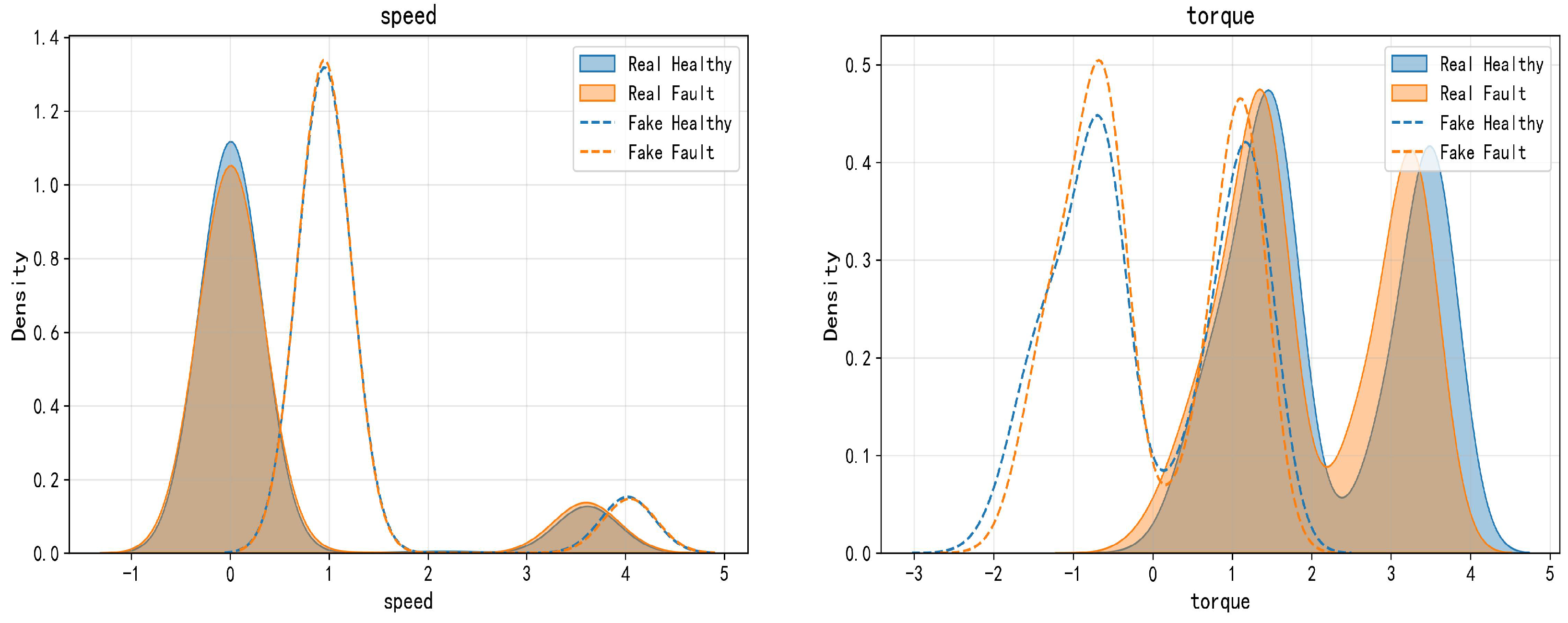
Ablation experiments show that the GAN + LSTM model attains a higher AUC than does the baseline GAN, reflecting enhanced discriminative capability and more realistic temporal feature modeling. We also visualized and analyzed the generated gear fault data. Figure 6, which uses kernel density estimation (KDE) plots, illustrates the overlap and separability between the two classes in the embedding space.

From the perspectives of data quality assessment and model performance, the AUC reaches 0.747, and the discriminator achieves a classification ACC of 0.809 on the generated samples, suggesting that the generator has successfully learned structural characteristics associated with faults. The KDE analysis primarily focuses on key operational variables of the gearbox: rotational speed and torque. For the GAN + LSTM model, KDE shows that the generated data reproduce the real-data statistical distributions, capture the fault-induced multimodal variations in speed, and emulate the high-load shifts in torque. The generated and actual density curves are highly similar in shape, peak position, and tail behavior. Therefore, the model can produce synthetic data with clear physical meaning and faithful statistical properties, supplying relatively high-quality data for downstream fault-detection tasks.

In summary, the proposed model’s effectiveness was validated from multiple perspectives, including KDE density plots and the discriminator’s classification accuracy. KDE analysis demonstrates that the statistical distribution of the generated data closely matches that of the real data, indicating that the model is capable of learning and reproducing fault-related dynamic characteristics. The discriminator attains 80.9% classification accuracy on generated samples, which is substantially higher than random chance, confirming that the synthetic data maintain strong semantic consistency. Integrating LSTM markedly improves the temporal coherence and physical plausibility of the generated sequences, making the GAN + LSTM framework better suited to industrial time-series fault data than MLP-based GANs. Consequently, the GAN + LSTM model can produce high-quality gear fault data that enhance fault diagnosis in small samples and thereby support intelligent industrial diagnostics.

4.4.2. Gated MoE Discriminator for Fault Detection

We replace the traditional discriminator (which uses a single feedforward network to map all inputs) with a multi-expert mixture mechanism governed by a gating network. The gated discriminative network comprises multiple expert subnetworks, each learning distinct local feature patterns (for example, different feature subspaces or combinations of vibration characteristics under varying operating conditions). The gating network assigns a weight to each expert, increasing model capacity while avoiding overfitting because only a subset of experts is activated for any given sample. In conditional GANs, the discriminator must both distinguish real from generated samples and classify sample labels (failure = 0/1). The gated structure lets the discriminator select experts according to category or feature subspace, enabling more sensitive judgments of the “pseudo-authenticity” of generated samples. Consequently, this yields richer and more stable gradient signals for the generator, mitigating common GAN training problems such as vanishing gradients and mode collapse. The mixture-of-experts (MoE) architecture integrated with a gating mechanism demonstrates ensemble learning properties. Within this framework, individual experts extract features from diverse perspectives, while the gating network performs soft voting by assigning adaptive weights. When combined with regularization techniques such as dropout and batch normalization, this architecture substantially enhances the model’s generalization capability.

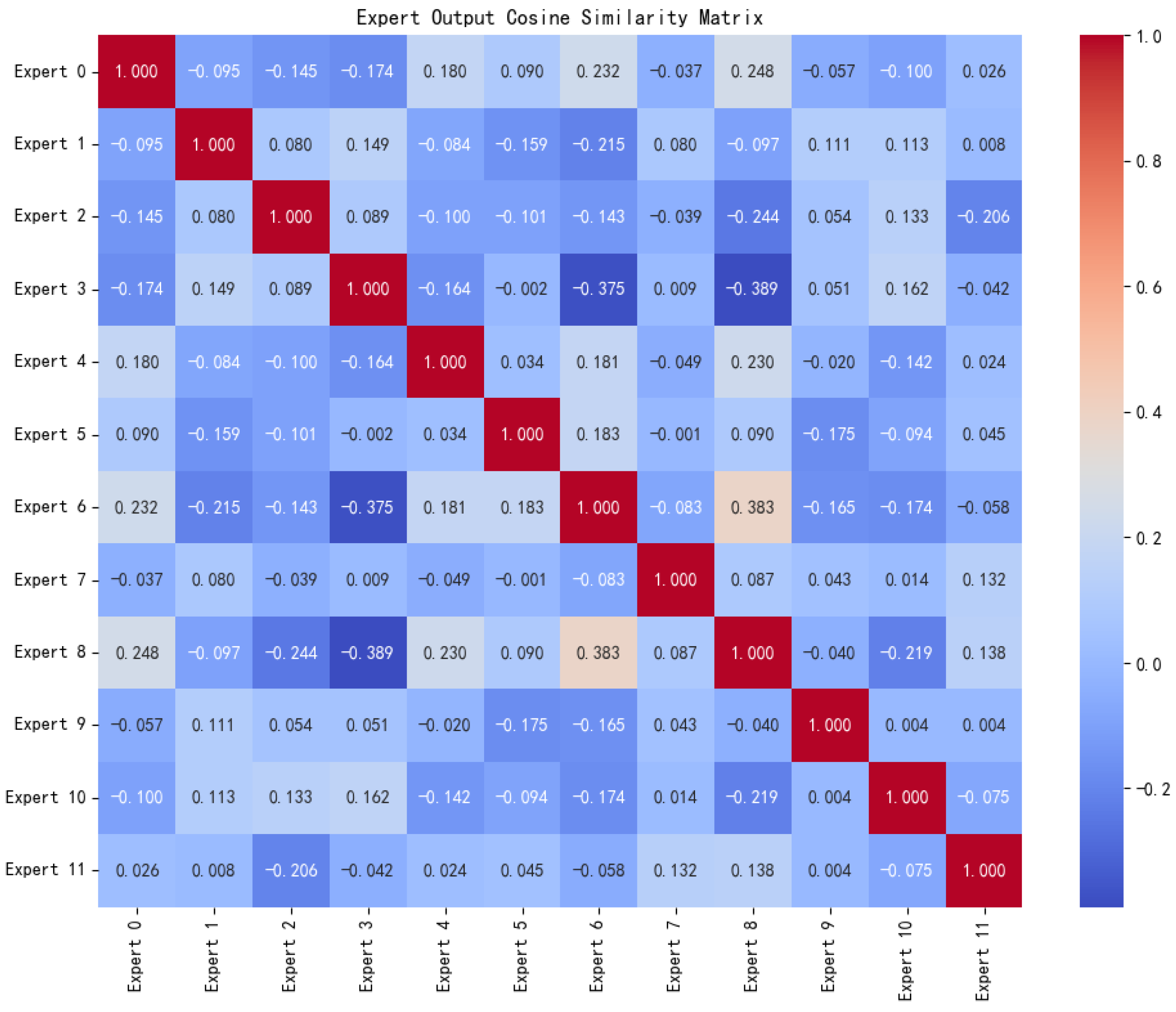
The incorporation of a gating network resulted in improved AUC and ACC values. As illustrated in Figure 7, the MoE architecture allows each expert to specialize in different data subpatterns, thereby promoting diversity and complementarity among the learned representations.

The experimental results illustrate the cosine similarity between the outputs of different experts. The generally low similarity values (approaching zero) and the absence of high redundancy (similarity > 0.7) suggest that the experts have diversified their representations rather than collapsing into identical mappings. While some pairs exhibit negative correlations, the primary observation is that the gating mechanism successfully encourages diversity among experts. This diversification allows the ensemble to cover a broader range of feature subspaces compared to a single discriminator, potentially contributing to the model’s robustness.

4.4.3. CNN-LSTM Fusion for Local-Global Feature Learning

For local pattern modeling, the generator input is “noise + label.” Inside the generator, the noise is treated as a pseudo-temporal signal and reshaped with unsqueeze into a 1D reshaped latent vector of shape [batch, 1, latent-dim + 1]. The CNN processes this pseudo-sequence to extract local correlations, capturing dependencies among adjacent dimensions of the noise vector. In contrast to multi-sensor time-series outputs of the model (for example, vibration signals along x, y, and z axes), measured data from real systems often exhibit local smoothness or periodicity. The Convolutional Neural Network (CNN), composed of convolutional and pooling layers, identifies basic features and combines them into higher-level hierarchical structures (such as periodic influences or harmonic components), enabling the generator to produce data that align with physical reality. In the CNN-LSTM hybrid architecture, the CNN extracts local spatial or short-range sequential features and supplies them to the LSTM for temporal modeling. This generative strategy better reflects the signal-generation mechanisms inherent to mechanical systems.

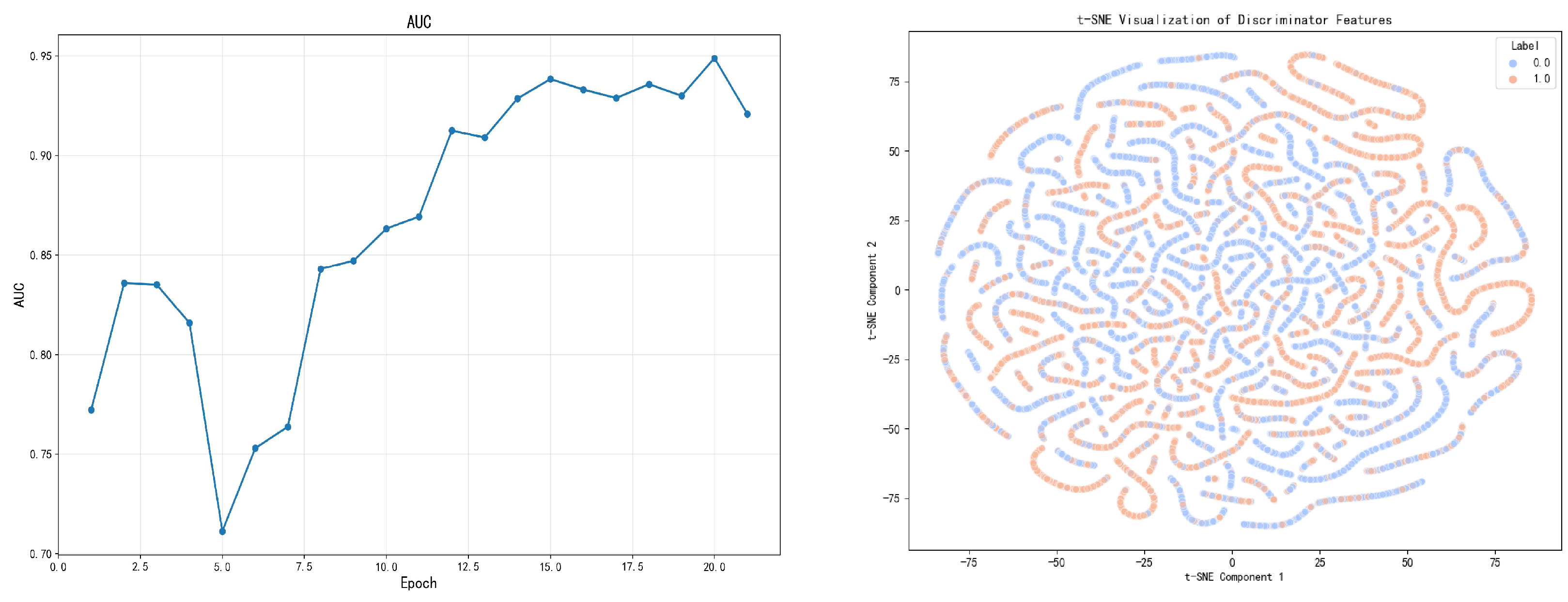
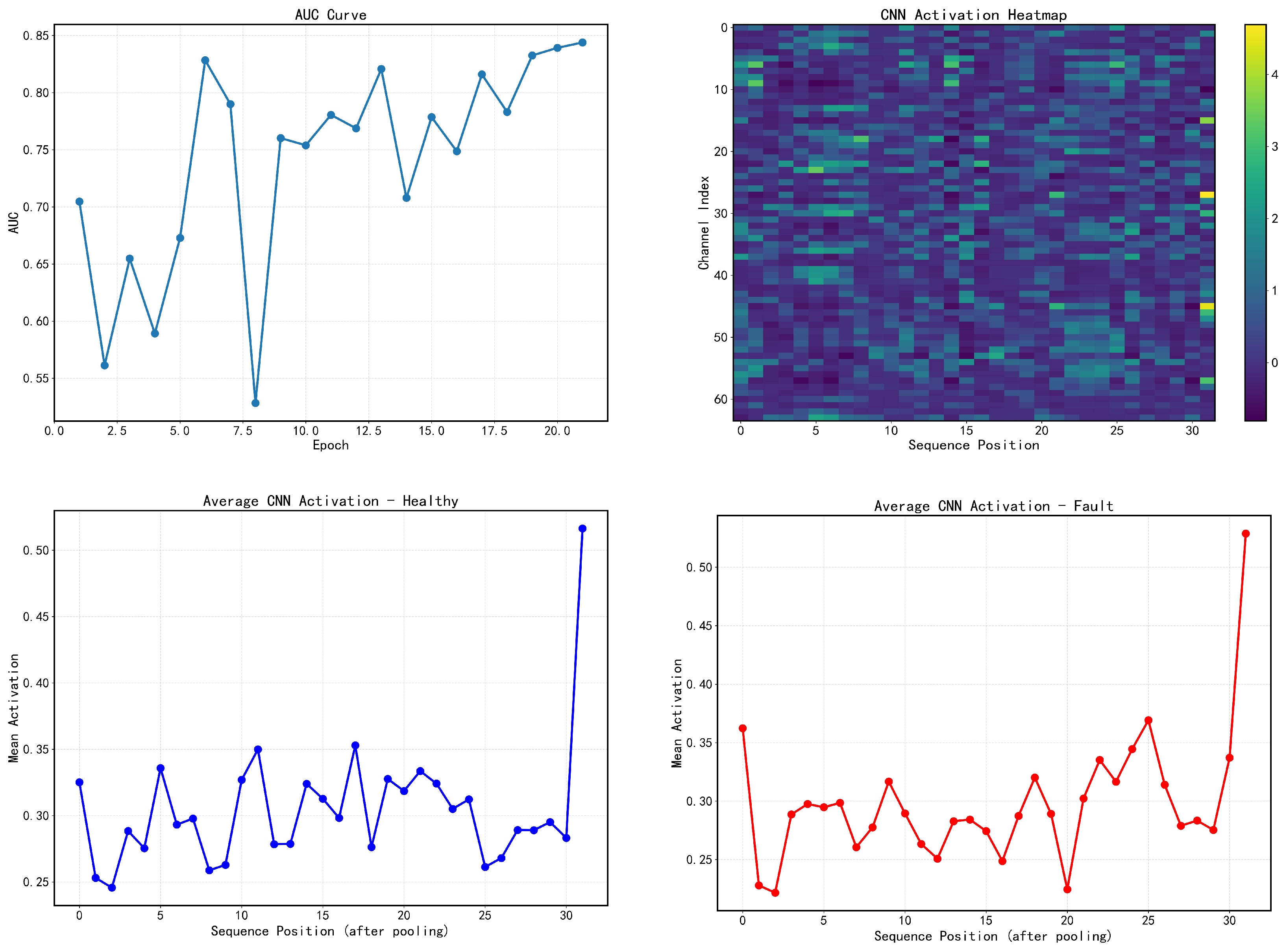
As shown in Figure 8, the minimum area under the curve (AUC) value was 0.54, with pronounced fluctuations observed during the first eight checkpoints (corresponding to the first 80 epochs). At the 21st checkpoint (corresponding to approximately the 200th epoch), the AUC value stabilized at around 0.85. In the AUC curve graph, the x-axis label 1–21 represents the checkpoint number, and the evaluation results are recorded every 10 epochs. Despite initial instability, the final performance indicates that the overall network, comprising CNN, LSTM, and mixture of experts (MoE), has strong modeling capability. The heatmap shows activation values across 128 convolutional channels and 31 sequence positions; brighter colors (yellow and green) denote stronger activation of a channel at a given position. The lack of continuous band-like or block-like high-response regions implies that the CNN did not learn dominant, rigid local motifs. Instead, most channels display modest responses, while a minority show relatively higher activation, indicating that the CNN captured combinations of latent variables and developed a discernible activation structure. A clear distinction appears near the end of the sequence, confirming that the CNN extracts a form of local dependency and uses it to separate healthy from faulty conditions. The averaged CNN activation curves encode class-specific information as distinct local patterns, and the eventual rise of AUC to 0.85 further validates that the CNN contributes meaningfully to overall model performance. The localized activation points in the heatmap also indicate that the CNN has learned local interaction patterns among latent dimensions. The marked difference in activation patterns at position 30 between healthy and faulty samples demonstrates the CNN’s ability to exploit local context for discrimination. Moreover, the non-overlapping activation curves across classes confirm that the CNN generates distinct responses to inputs from different categories.

4.4.4. Clustering-Guided Structure-Aware Generation

Raw signals exhibit complex distributional structure that binary labels (0/1) do not fully capture. We apply PCA and K-means clustering to discover latent geometric partitions in the feature space. Metadata shows that the resulting clusters ($K=2$, silhouette $=0.27$) separate primarily by speed ($F=9.91\times {10}^6$, $p<0.001$) rather than load ($F=0.31$, $p=0.58$) or fault labels (${\chi }^2=1.56$, $p=0.21$). Therefore, these clusters reflect data-driven distributional structure rather than predefined physical regimes. Nevertheless, incorporating distance-to-centroid features improves model performance by encoding each sample’s topological position in latent space, providing the discriminator with richer geometric context (ablation study shows AUC gain on MCC5). The circular t-SNE pattern further suggests that the model learns a continuous degradation manifold rather than discrete fault categories, which the MoE gating mechanism can exploit for adaptive feature routing. As a result, decision boundaries become more precise, and heterogeneous samples are less likely to be grouped into the same class, which would otherwise produce ambiguous decisions. Sequential feature engineering captures temporal dynamics because gearbox states evolve over time (for example, vibrations that increase gradually). We generate first-order difference, cumulative mean, normalized change rate, and other time-series features, so the model can approximate trends even without access to original time-series windows. These enhancements supply CNN-LSTM generators with richer dynamic priors, helping synthetic data to match real data not only in static distributions but also in patterns of change. The gating network (MoE) synergizes with structured inputs to enhance representational capacity. A single neural network struggles to model multiple fault modes simultaneously; however, our framework’s discriminator employs an expert network. When inputs include clustering information, the gating network more easily learns strategies such as “different clusters correspond to different experts,” achieving conditional specialization where each subpattern is managed by a dedicated expert.

As shown in Figure 9, the distribution map plotted by reducing the dimensionality of intermediate discriminator features via t-SNE exhibits a circular structure, in which blue samples (healthy condition) and orange samples (faulty condition) are intertwined. This visualization demonstrates that the model has acquired complex nonlinear decision boundaries instead of being restricted to simple linear classification, which is consistent with the high AUC value obtained by the model. The MoE structure can assign feature extraction tasks to different degradation stages and hand them over to specially trained experts for processing so that even without global category separation, the model can capture local discriminative clues. From a visual perspective, this configuration can generate high-quality synthetic data and reveal the structure of the data. Although clusters reflect speed rather than fault labels, this aligns with gearbox physics where fault signatures are speed-modulated. Topological priors help the MoE discriminator learn and operate within the fault boundaries related to the operating conditions, enabling MoE to learn speed-adaptive fault boundaries.

4.5. Parameter Sensitivity Analysis

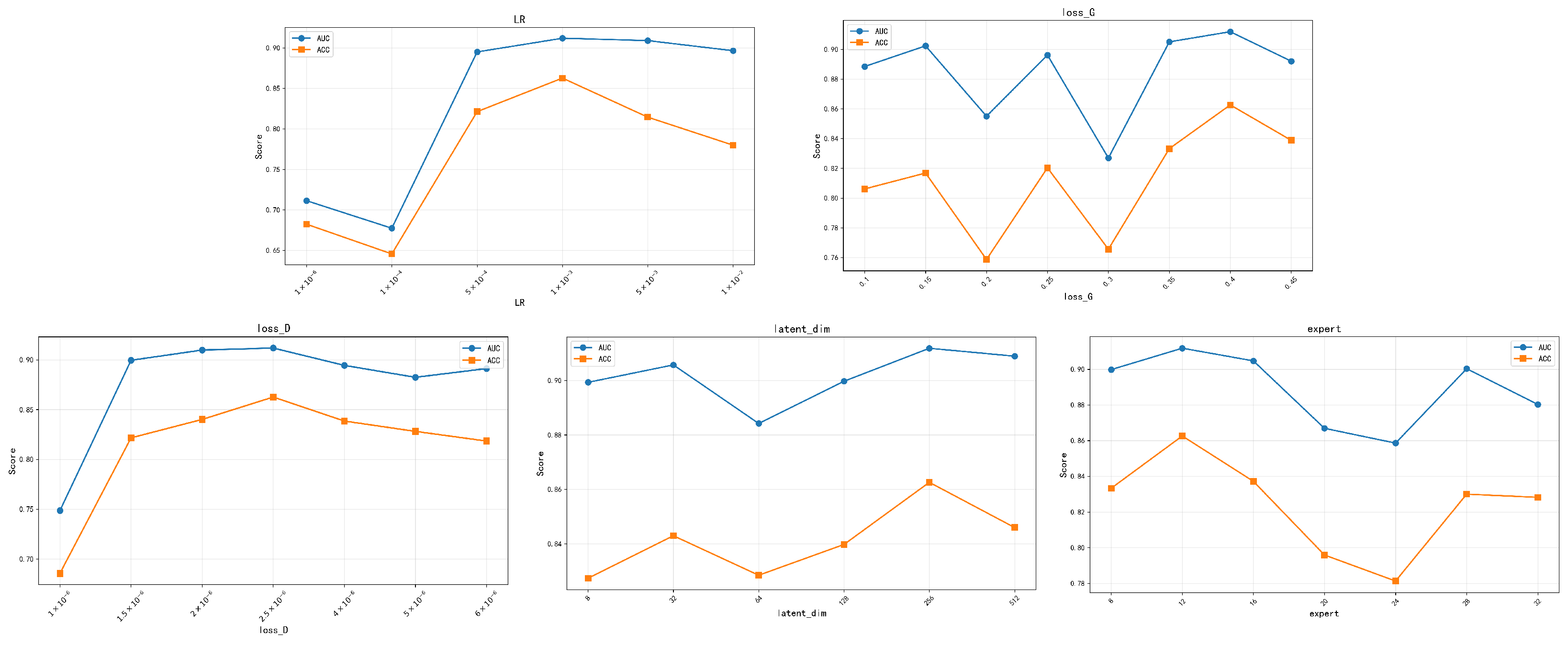
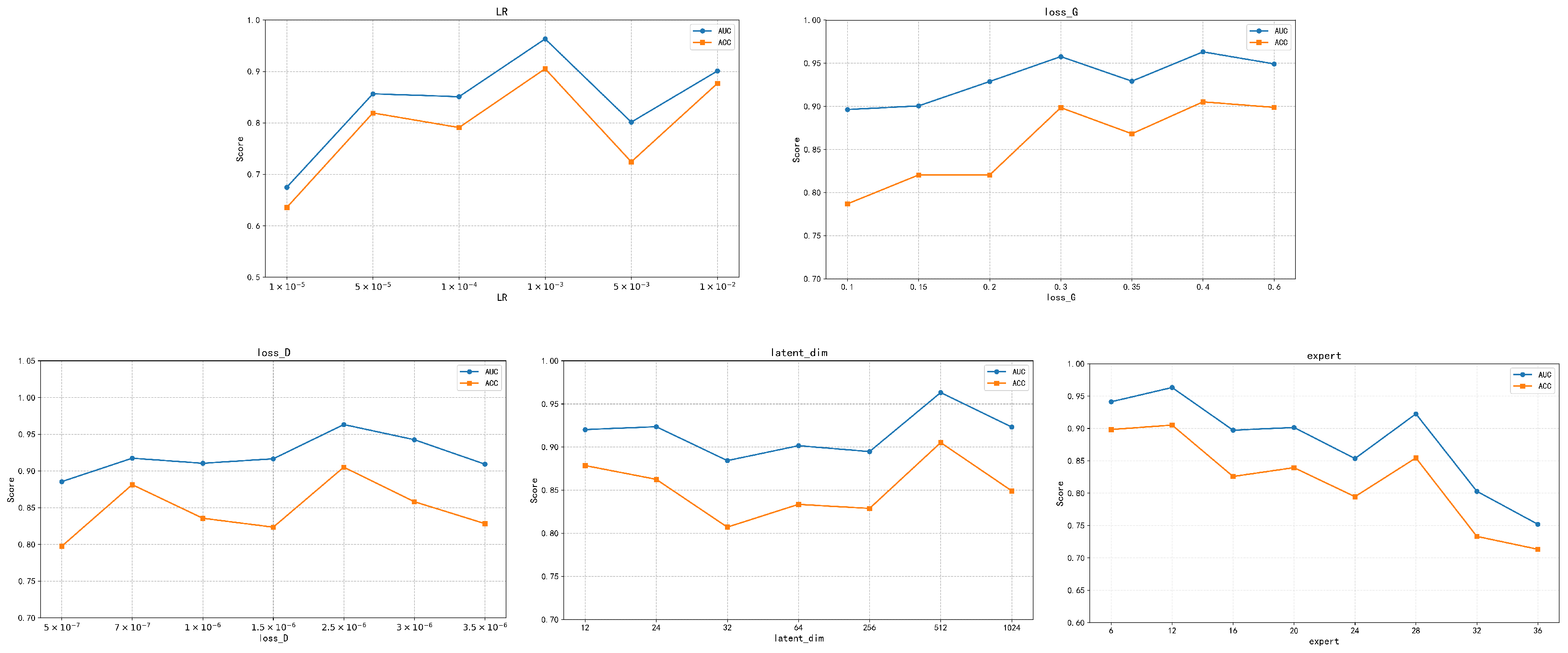
In this study, we used AUC and ACC as evaluation metrics to perform a sensitivity analysis of hyperparameters on two representative gearbox fault diagnosis datasets. We focused on five core parameters: latent space dimensionality, number of expert networks, discriminator classification loss weight, generator classification loss weight, and optimizer learning rate. Each parameter was varied in the corresponding fault classification and recognition tasks. We then analyzed the specific effects of these hyperparameters on the overall model. Results are presented in Figure 10 and Figure 11.

The two parameters (latent-dim and expert) decide the model feature representation capability and the diversity of expert routing. The experiments show that both have a very “inverted U” curve. In the Gearbox Fault Diagnosis dataset, the peak is reached when latent-dim is 256, and in the more complex MCC5 dataset with more features, the best latent-dim is 512. It can be seen that the latent space dimension needs to be matched with the complexity of the data. The optimal number of experts is 12 in both datasets. An appropriate expert scale can ensure the specificity of features while effectively avoiding the problems of low expert utilization and routing redundancy.

The direct weight of the adversarial loss determines (loss-D and loss-G) the balance of game between generator and discriminator. Low loss-D leads to incomplete adversarial supervision and random guessing, and high loss-G disrupts training stability. Stronger generator signal and weak but stable discriminator feedback are the best combination for maintaining dynamical balance between adversarial training and generalize very well across datasets.

Learning rate is the most sensitive test parameter. LR = 0.001 achieves the best convergence speed and training stability on both datasets (especially MCC5 dataset). Except the one which needs to be adaptively adjusted according to the complexity of the data set (latent-dim), all other four parameters behave exactly the same on two very different data sets, demonstrating the robustness and cross-domain transferability of the hyperparameter configuration of the proposed model. To ensure statistical rigor, the comparative experiments reported in Table 1 were repeated with multiple predefined random seeds. On the MCC5 dataset, TGME-GAN achieves $\mathrm{Accuracy}=0.8614\pm 0.0114$ and $\mathrm{AUC}=0.9128\pm 0.0132$; on the Gearbox Fault Diagnosis dataset, it achieves $\mathrm{Accuracy}=0.9022\pm 0.0151$ and $\mathrm{AUC}=0.9611\pm 0.0147$. Compared to the strongest baseline MHTA-DDPM, TGME-GAN improves AUC by $0.87\%$ on MCC5 while achieving substantially better accuracy on Gearbox Fault Diagnosis ($+2.37\%$). The low standard deviations across all methods demonstrate stable performance. Regarding computational cost, the 12-expert MoE discriminator contains $0.71$ M parameters (Gearbox) and approximately $1.1$ M parameters (MCC5), with the generator contributing $0.13$ M, totaling $0.84$ M and approximately $1.2$ M respectively. Training was conducted on an Intel i5-14400 CPU with Python 3.8; each epoch required approximately 180 s (Gearbox) or 200 s (MCC5), with a total training time of approximately 10 h over 200 epochs. Inference latency was $0.21$ ms per sample on CPU, meeting real-time requirements for industrial monitoring. Expert utilization analysis shows an average routing probability of $8.33\%$ per expert (theoretical uniform distribution), with maximum usage at $18.55\%$ and minimum at $2.88\%$, confirming balanced specialization without collapse. The combination of dropout ($0.5$), gradient clipping ($\parallel \nabla \parallel \le 0.5$), and early stopping via ReduceLROnPlateau effectively mitigates overfitting, as evidenced by the relatively small standard deviations of the proposed TGME-GAN across the repeated runs.

4.6. Comprehensive Multi-Dimensional Validation of Model Optimality

To fully validate TGME-GAN, we evaluated its diagnostic performance, the fidelity of the synthesized data, and the training stability on the GFD and MCC5 datasets. The comprehensive indicators reported in this section (PR-AUC, F1 score, sensitivity, specificity, synthetic data quality indicators, and training dynamics) are based on the results of a single representative training run with a random seed of 42. On the GFD dataset, the model achieves a PR-AUC of 0.9531, an F1-score of 0.8998, a sensitivity of 0.9138, and a specificity of 0.8833. The false-positive rate (FPR) is 0.1167 and the miss rate is 0.0862. Precision reaches 0.8862, confirming low false alarms. On MCC5, the PR-AUC is 0.8903, the F1-score is 0.8491, the sensitivity is 0.8516, the specificity is 0.8671, the FPR is 0.1329, the miss rate is 0.1484, the accuracy is 0.8626, the ROC-AUC is 0.9118, and the precision is 0.8466. For synthetic data quality, MMD values are 0.1211 (GFD) and 0.2829 (MCC5). FID-style distances are 11.86 (GFD) and 39.22 (MCC5). Average Wasserstein distances are 0.4258 (GFD) and 0.7162 (MCC5), with per-feature ranges of 0.0292–0.6085 (GFD) and 0.1424–0.9520 (MCC5). Variance ratios (Fake/Real) are 1.0721 (GFD) and 0.8309 (MCC5); real/generated variance/std averages are 0.9895/0.9939 vs. 1.0609/1.0280 (GFD) and 1.0965/1.0333 vs. 0.9110/0.9358 (MCC5). Class-conditional coverage for fault samples is 0.0730 (GFD) and 0.0350 (MCC5), with healthy coverage at 0.0770 and 0.0010, respectively. Downstream classification accuracy using only synthetic data reaches 0.9260 (GFD) and 0.9010 (MCC5). Training dynamics show stable convergence. On GFD, peak AUC of 0.9725 occurs at epoch 110; learning rate reductions at epochs 7, 13, and 19 ensure smooth optimization. Final evaluation yields an accuracy of 0.9051 and an of ROC-AUC 0.9631. On MCC5, AUC stabilizes above 0.92 after epoch 130, with a final accuracy 0.8626 and an ROC-AUC 0.9118. Adaptive learning rate scheduling prevents divergence throughout 200 epochs on both datasets. In summary, the consistently high PR-AUC and F1-scores across both datasets confirm the model’s robustness to distribution heterogeneity and limited fault representation in industrial fault diagnosis. The reported MMD/FID-style distances and near-unity variance ratios suggest that the generated samples retain aspects of the real-data distribution and variance. Stable training convergence with adaptive learning rate scheduling further validates the architectural reliability of TGME-GAN, collectively proving its optimality for gearbox fault diagnosis under heterogeneous operating conditions.

5. Conclusions and Future Work

This paper proposes a gearbox fault diagnosis method based on a Time-Gated Multi-Expert Generative Adversarial Network (TGME-GAN). The method addresses core challenges in industrial gearbox diagnosis, including complex multi-scale temporal patterns, distribution heterogeneity across operating conditions, and limited labeled samples, by constructing a hybrid generative framework. The main methods adopted in this paper are as follows: (1) a multi-scale sequence enhancement strategy, (2) an innovative generator architecture, (3) a dual-task discriminator mechanism, and (4) data generation based on enhanced clustering features. (1) The multi-scale sequence enhancement strategy integrates differential features, cumulative statistics, normalized rate-of-change sequences, and structural information extracted by PCA-based dimensionality reduction followed by K-means clustering. The resulting high-dimensional enhanced feature space jointly encodes original operating variables, dynamic evolution trends, and latent state partitions. (2) Regarding the innovative generator architecture, the generator is redesigned as a CNN-LSTM joint encoder. One-dimensional layers capture local temporal patterns, while an LSTM module models long-range dependencies. (3) The dual-task discriminator mechanism employs a framework based on the traditional MoE structure with a shared gating unit, enabling simultaneous discrimination between real and synthetic samples while performing fault classification. The integration of adversarial training with supervised learning significantly enhances model stability. (4) For data generation based on enhanced clustering features, the K-means clustering labels and the distance between centroids are used as auxiliary input features for the discriminator, enabling the discriminator to distinguish the consistency of real samples and synthetic samples in the clustering distribution and guiding the generator to synthesize fault samples that are more in line with the actual data distribution.

TGME-GAN not only boasts outstanding classification accuracy but also breaks through the traditional classification paradigm at three core levels: scalable reasoning, cognitive diagnostic capabilities, and industrial robustness. Scalable reasoning is achieved through a modular hybrid expert discriminator that supports incremental expansion and the ability to adapt to new working conditions and fault modes without model reconstruction. After expansion, the recognition performance steadily improves. Cognitive diagnostic capabilities include relying on the embedding of cluster structures to establish hierarchical cognitive mechanisms, empower discriminative learning through cross-domain topological priors, and conform to the human logic of anomaly identification from the global to the local. Regarding industrial robustness, the unified generation discriminant architecture is adapted to multiple types of heterogeneous industrial data. It performs stably in complex scenarios such as category imbalance and distribution shift, significantly outperforming traditional classifiers and two-stage GAN methods. At the same time, relying on the modular MoE discriminator, the structure can be flexibly expanded. By adding a new expert subnet, it can adapt to various new working conditions and faults. The clustering structure is embedded to build a hierarchical cognitive diagnosis link, and the cross-domain transfer of topological prior assists in discriminative learning, replicating the abnormal human identification thinking from the whole to the part.

The experimental results on the gearbox health monitoring dataset show that the proposed method can effectively accomplish the fault diagnosis task. Although the method proposed in this paper has achieved favorable results in several aspects, numerous areas remain to be explored and improved. To enhance the model’s generalization capability, meta-learning techniques could be incorporated, as the current model—specifically trained for gearbox fault diagnosis—is limited in its adaptability across different equipment types and operational conditions. Regarding real-time inference requirements, subsequent research could adopt knowledge distillation, model pruning, and lightweight MoE designs to reduce deployment costs and meet edge computing demands. Future work may explore nonlinear manifold clustering methods such as spectral clustering or deep clustering to better capture complex fault structures under varying operating conditions. In conclusion, the TGME-GAN model proposed in this paper provides a new approach for fault diagnosis in industrial intelligent operation and maintenance.