Federated Learning-Based Adaptive Multi-Head Attention Model for Wind Power Forecasting

Abstract

Enhancing the accuracy of short-term wind power forecasting helps mitigate the adverse impacts of prediction errors on grid dispatch. Wind power exhibits a significantly nonlinear dependence on multiple influencing factors. However, existing methods struggle to effectively resolve multi-dimensional feature redundancy and multi-scale non-stationary evolutionary characteristics inherent in far-offshore wind power forecasting tasks. This leads to bottlenecks such as insufficient feature discriminability and temporal dependency focus shift under complex marine environments, ultimately limiting further improvements in prediction accuracy. To address these challenges, this paper proposes a federated learning-based adaptive multi-head attention model for wind power forecasting (Fed-AMHA). The proposed framework operates as follows: First, each wind farm client utilizes a Bidirectional Long Short-Term Memory (BiLSTM) network to model input sequences bidirectionally, capturing long-term temporal dependencies. Subsequently, linear projection and parallel one-dimensional convolution operations are introduced to mine multi-scale local temporal features from each time step and its neighborhood. Building upon this, channel attention and multi-head temporal feature attention mechanisms are stacked. The model adaptively adjusts the weights of different time slices and feature channels by learning the importance of each channel to the forecasting task. The central server then aggregates the model parameters uploaded by the clients via averaging, enabling cross-site collaborative training without directly sharing raw data. Simulation results based on public datasets and actual wind farm data under various short-term forecasting scenarios demonstrate that the proposed model consistently achieves lower prediction errors and superior stability compared to existing forecasting models under identical settings.

1. Introduction

With the continuous development of society and the ever-increasing demand for energy, traditional power grids relying on fossil fuels for electricity generation produce greenhouse gas emissions, leading to global warming. This reality is thus driving the transition towards Smart Grids [1]. Due to its cost-effectiveness, availability, and environmental friendliness, wind energy has emerged as a crucial form of clean and renewable energy. However, wind energy is inherently intermittent, stochastic, and uncontrollable. Consequently, wind power generation is comprehensively influenced by multiple factors, including the physical design of wind turbine blades, the technical specifications of the turbines, geographical location, and the climatic conditions of the area. Under the combined influence of these multifaceted factors, the stability of wind power output is significantly compromised, leading to difficulties in power dispatch. Accurate short-term forecasting of wind power based on historical wind resource data from wind farms is beneficial for the timely and rational planning of wind energy development, improves the quality of power supply, and simultaneously reduces wear and tear on wind turbines, thereby cutting costs and minimizing resource waste [2].

With the construction of onshore and nearshore wind farms approaching saturation and available development space becoming limited, the global focus of wind power generation is shifting from land and nearshore areas towards the far-offshore regions, which boast more abundant resource reserves. Far-offshore areas possess more expansive maritime space and superior wind energy resources, making them the primary zones for future wind energy development. However, far-offshore wind farms are located far from coastlines and endure harsh environmental conditions, meaning equipment wear or errors in power dispatch can lead to significant economic losses. Consequently, conducting research on far-offshore wind power forecasting is not only an urgent requirement for coping with extreme conditions in these areas and ensuring the reliable power supply capacity of the grid but also represents the core of achieving refined operation and management for far-offshore wind power generation. Current short-term wind power forecasting methods are primarily categorized into physical methods, statistical methods, and machine learning (ML) methods [3].

Physical methods primarily rely on terrain, roughness, wind farm layout, and the characteristic parameters of wind turbines. They utilize micro-meteorological theory and fluid dynamics to establish models for describing wind energy resource distribution [4]. These methods do not depend on historical data from wind power sites, making them suitable for wind farms under construction or those lacking data. However, this approach requires simulating changes in meteorological elements such as local wind speed and wind direction, leading to extremely high modeling complexity and uncertainty, which can introduce further systematic bias. In comparison to physical methods, statistical methods are simpler and rely on a limited scope of data. They are primarily based on modeling historical time-series data [5]. Methods such as the Autoregressive (AR) model [6], Autoregressive Moving Average (ARMA) model [7], and Autoregressive Integrated Moving Average (ARIMA) model [8] typically characterize the dynamic features of wind power based on single-variable wind power data. The Vector Autoregression (VAR) model [9] assumes linear dependencies among variables. The computational cost of Gaussian Process (GP) models [10] grows exponentially with data volume. Due to the exponential growth in model complexity with the number of variables in statistical methods, they suffer from being computationally inefficient, having high computational complexity, and exhibiting low accuracy in linear predictions. Consequently, the applicability of these methods is often limited in newly constructed or data-scarce wind farm sites [11].

In recent years, the advancement of deep learning has broken through the limitations inherent in physical and statistical methods. Nonlinear modeling techniques and machine learning approaches have demonstrated significant potential in wind power forecasting tasks. Owing to its outstanding capability in extracting temporal features, Long Short-Term Memory (LSTM) networks and convolutional neural networks (CNNs) have achieved remarkable success in forecasting tasks. Within the field of wind power forecasting, numerous research efforts have yielded substantial progress based on LSTM. Studies [12,13] utilized attention mechanisms combined with other networks to construct hybrid models, thereby enhancing the accuracy of wind power forecasting. Similarly, works [14] further improved forecasting accuracy by introducing LSTM to extract temporal features from historical wind power data. Although centralized machine learning has exhibited excellent performance in terms of accuracy for wind power forecasting tasks, it operates under the assumption that data from various wind power sites can be transmitted and aggregated centrally. This assumption is often difficult to fulfill in practical forecasting scenarios, primarily for three reasons: First, the harsh environment of far-offshore wind farms makes it challenging to establish reliable communication links between sites, resulting in data typically existing in isolated forms at each location. Second, far-offshore wind power data involves national security and commercial competition concerns, where data transmission carries risks such as privacy leakage. Third, meteorological data from different sites within a far-offshore wind farm exhibit significant differences in the feature space and are non-independently and identically distributed (non-IID). Training a single global model using aggregated data would cause the model to lean towards learning the average features of all sites, severely degrading the forecasting performance for specific sites located in extreme climate zones. To address the issues mentioned above, the forecasting method based on federated learning (FL) [15] trains models on the local data of each site independently, eliminating the need to upload data to a central server for centralized training. This approach not only ensures data privacy and prevents leakage but also reduces the computational resources required by the server. Consequently, it holds significant advantages for far-offshore wind power forecasting tasks. Moradzadeh et al. [16] proposed a CNN-based federated learning framework for forecasting photovoltaic power generation in different regions. Building upon the architecture in [2], Loukil et al. [17] introduced a federated learning framework combining CNNs and LSTM for wind power forecasting. Zhang et al. [18] proposed a novel federated learning model for predicting wind turbine blade icing based on a feature enhancement selection method utilizing prior knowledge. However, the aforementioned methods struggle to effectively address the challenges posed by multi-dimensional feature redundancy and multi-scale non-stationary evolution in far-offshore wind power forecasting. This limitation restricts the model’s ability in key feature identification and temporal dependency modeling under complex marine environments, making it difficult to support high-precision forecasting requirements.

To address the aforementioned challenges, this paper proposes a federated learning-based adaptive multi-head attention model for short-term wind power forecasting at distributed sites within far-offshore wind farms. The main technical contributions of this work are summarized as follows:

• A parallel temporal feature-enhanced BiLSTM model framework for deep-sea offshore wind power forecasting is proposed. To address the strong non-stationarity and multi-scale temporal dependence characteristics of deep-sea offshore wind power time series, a Top-K feature selection method based on Spearman’s rank correlation is first employed for data dimensionality reduction. Subsequently, a BiLSTM is utilized to extract long-range bidirectional temporal dependencies, while a multi-branch 1D-CNN structure is constructed in parallel, thereby enhancing the model’s capability to characterize complex time-series evolution patterns.
• An adaptive feature recalibration mechanism based on channel attention is designed. By dynamically modeling the importance of multi-channel temporal features and utilizing the query vector $h_{last}$ generated by mapping the final hidden state of the BiLSTM as guidance, the contribution of each channel branch is adjusted. This suppresses redundant and noisy information, improves the discriminability and robustness of the model’s feature representation, and enhances its generalization capability in complex marine environments.
• An adaptive multi-head temporal attention mechanism is introduced to precisely focus on critical historical information. Unlike traditional direct concatenation, learnable head weights are incorporated for aggregation. By aggregating these weights based on the importance of different heads exhibited during the learning process, fine-grained modeling of essential time-series information is achieved, thereby significantly enhancing forecasting accuracy and stability. Validation on two public datasets demonstrates that the proposed model effectively improves the prediction accuracy of wind power generation.

The rest of this paper is organized as follows. Section 2 provides a brief review of related research on feature selection and wind power forecasting. Section 3 articulates the statement of the research problem. Section 4 elaborates in detail on the proposed wind power forecasting model based on Spearman’s rank correlation coefficient and adaptive multi-head attention. Section 5 introduces the comparative experiments and analyzes the corresponding results. Section 6 concludes the work presented in this paper.

2. Related Work

2.1. Feature Selection

The accuracy of wind power forecasting is highly dependent on the quality of the input features. The raw data collected from various sites within a wind farm typically contain a large number of high-dimensional and redundant features. If left unprocessed, this raw data not only triggers the “curse of dimensionality” and degrades the model’s generalization capability but also introduces interference that adversely affects the forecasting model’s accuracy. Feature selection, owing to its ability to reduce data dimensionality and eliminate redundant or duplicate information, thereby enhancing model generalization, has been widely adopted as a crucial data preprocessing step in forecasting tasks. Effective feature selection methods ensure that forecasting models can identify and retain the most relevant features from the dataset, consequently improving both the accuracy and efficiency of the model. Numerous feature selection techniques have been employed in energy forecasting tasks, including Pearson Correlation Coefficient (PCC) [19] Euclidean Distance (ED) [20], Principal Component Analysis (PCA) [21] and eXtreme Gradient Boosting (XGBoost) [22].

Thipwangmek et al. [23] conducted a comparative study on short-term solar photovoltaic forecasting using LSTM models integrated with four distinct feature selection methods: PCC, ED, PCA, and XGBoost. Their experimental results demonstrated that the PCC-LSTM model achieved optimal performance, yielding the lowest Root Mean Square Error (RMSE) and Mean Absolute Error (MAE) values. Ge et al. [24] proposed an adaptive feature screening framework for probabilistic multi-energy load forecasting. By integrating multi-quantile regression models with residual-connected Lasso methodology, they developed the ProbLassoNet model, which simultaneously accounts for both linear and nonlinear components to enable effective feature selection. Validation on public datasets confirmed the significant effectiveness of this approach. Yang et al. [25] proposed a hybrid forecasting framework that integrates Pearson Correlation Coefficient analysis with BiLSTM. Their model significantly outperformed existing approaches including standalone LSTM and BiLSTM models in terms of both forecasting accuracy and reliability. However, these methods generally exhibit limitations in fully characterizing the dynamic coupling relationships among multi-dimensional features and their time-varying non-stationary characteristics during the feature selection and modeling processes. Consequently, their adaptability and effectiveness in wind power forecasting tasks require further enhancement.

2.2. Wind Power Forecasting Models

One of the primary research focuses in the wind energy domain involves short-term wind power forecasting for distributed sites based on historical power data and multi-source meteorological information. Liu et al. [26] proposed a Multi-Task Temporal Feature Attention LSTM (MTTFA-LSTM) model that integrates historical power generation data with diverse meteorological sources. This framework synergistically combines LSTM, CNN, and attention mechanisms to model multi-step temporal characteristics, demonstrating superior performance over baseline models under identical conditions. Yu et al. [27] developed an enhanced forecasting framework incorporating CNN, BiLSTM, and attention mechanisms. Experimental results indicate that their model achieves higher prediction accuracy and improved stability. Rahmatinia et al. [28] introduced a deep learning methodology based on an encoder–decoder architecture integrated with attention mechanisms for the simultaneous prediction of key parameters in power systems. This approach attained notably higher forecasting precision compared to conventional methods. The heavy reliance of centralized methods on unified data acquisition poses significant challenges for their practical deployment and large-scale expansion in far-offshore environments, where wind turbines are geographically dispersed and communication bandwidth is constrained.

Current research has seen some investigators exploring distributed forecasting tasks within federated learning frameworks, achieving certain progress. Shivkumar et al. [29] proposed a Transformer model trained using federated learning, which addresses privacy protection while performing wind power forecasting. Experimental results show that this model performs better in terms of RMSE values and prediction accuracy. Rahman et al. [30] introduced a computationally efficient and attack-resistant federated learning scheme that improves efficiency by reducing the number of client models participating in federated aggregation. Experimental results indicate that this scheme can enhance computational efficiency by up to 60% during model training and server transmission processes. Liu et al. [31] proposed a pattern-measurement collaborative interaction framework that deeply integrates physical and data-driven models through learnable operators and incorporates federated split learning, effectively alleviating data privacy and secure collaboration challenges during training across sites in large-scale wind farms. Jayashri et al. [32] presented a multi-source heterogeneous information fusion scheme leveraging cross-attention mechanisms within a federated framework, which achieved strong prediction accuracy on renewable energy datasets. Nevertheless, current federated prediction models lack adequate analysis of feature redundancy and non-stationary properties in far-offshore data, resulting in feature discrimination deficiencies and temporal attention deviations that hinder predictive accuracy improvements.

3. Problem Restatement

Wind resources are inherently characterized by significant randomness, intermittency, and uncertainty, which render wind power output with strong nonlinear and non-stationary features and pose considerable challenges to the dispatching and operation of power systems. Therefore, how to achieve high-precision short-term wind power forecasting based on historical observation data has become one of the core issues in the grid-connected operation of wind power.

Let the multi-dimensional observation feature vector of the wind farm at time step t be expressed as

$$x_t\in {\mathbb{R}}^d$$

(1)

where d denotes the number of features, which usually includes variables closely related to wind power output, such as wind speed, wind direction, temperature, air pressure, and humidity. For a historical time window $[t,t+p-1]$ of length p, the model input can be expressed as a multivariate time series:

$$X_t={\left[x_t,x_{t+1},\dots ,x_{t+p-1}\right]}^{\mathrm{T}}\in {\mathbb{R}}^{p\times d}$$

(2)

The goal of short-term wind power forecasting is to learn a nonlinear mapping function $f(·)$, such that the model can predict the wind power output at the next time step based on the historical observation sequence $X_t$:

$$\widehat{y}=f\left(X_t\right)$$

(3)

where $\widehat{y}$ denotes the predicted value of wind power at the future time step.

In practical applications, due to the wide distribution of wind farms and their affiliation with different operating entities, raw data is often restricted by privacy policies and commercial secrets, making it impossible to be directly aggregated to the cloud, thus forming “data silos”. Federated learning provides a solution for collaborative modeling while ensuring that data does not leave the local site. Assume there are K wind farm participants in the federated network, where each participant $k\in \{1,2,\dots ,K\}$ holds its local dataset $D_k$. The goal of federated short-term wind power forecasting is to collectively learn an optimal global mapping function $f(X;\theta )$ by aggregating the model updates from each site via a server. Its local loss function ${\mathcal{L}}_k\left(\theta \right)$ is defined as the discrepancy between the local predicted value and the true power value y at that site:

$$\begin{array}{cc}\hfill {\mathcal{L}}_k\left(\theta \right)& ={\displaystyle \frac{1}{n_k}}{\displaystyle \sum _{i=1}^{n_k}}{\left|{\widehat{y}}_i^{\left(k\right)}-y_i^{\left(k\right)}\right|}^2={\displaystyle \frac{1}{n_k}}{\displaystyle \sum _{i=1}^{n_k}}{\left|f\left(X_i^{\left(k\right)};\theta \right)-y_i^{\left(k\right)}\right|}^2\hfill \end{array}$$

(4)

where $n_k$ is the number of samples at the k-th site. The global optimization objective of federated learning is to find a set of parameters $w^{\ast }$ that minimizes the weighted sum of losses of all participants on their respective private data:

$$\underset{w}{\min }F\left(w\right)={\displaystyle \sum _{k=1}^K}{\displaystyle \frac{n_k}{N}}{\mathcal{L}}_k\left(\theta \right)$$

(5)

where $N=\sum n_k$ is the total number of samples.

This forecasting task faces multiple key challenges: the highly nonlinear and time-varying relationship between wind power and meteorological variables—shaped by terrain, airflow, and climate—resists capture by traditional linear models; the dynamically changing influence of different meteorological features requires accurate modeling of heterogeneous feature relationships; wind power’s combination of long-term trends and short-term fluctuations demands effective capture of multi-time-scale dependencies; and the unequal contribution of historical time steps necessitates adaptive identification of critical time segments and relevant feature patterns to enhance forecasting accuracy and robustness.

Based on the above analysis, this paper models the wind power forecasting problem as a multi-variable, multi-time-scale time-series regression task, aiming to achieve accurate prediction of short-term wind power output by effectively mining the temporal dependency relationships and feature importance information in historical observation data. The following table is cited to explain the main symbols used in this paper, as shown in

Table 1. Definition of symbols.

Symbol	Explanation
$x_t$	Multi-dimensional observation feature vector at time step t
d	Number of features
$[t,t+p-1]$	Historical time window with length p
$X_t$	Multivariate time series
$\widehat{y}$	Wind power forecast value
n	Total number of time steps
A	Feature matrix
y	Target variable
$a_j$	j-th feature column
${\rho }_j$	Spearman’s rank correlation coefficient between feature and target variables
S	Feature subset
K	Total number of selected features
$A_S$	Selected feature matrix
$f_t$	Forget gate
$i_t$	Input gate
${\tilde{C}}_t$	Candidate memory cell
$o_t$	Output gate
H	Hidden state matrix
C	Convolution kernel matrix
$c_j$	j-th 1D convolution kernel
a	Channel importance weight
G	Output matrix of parallel sublayer
z	Channel description vector
$\tilde{G}$	Feature sequence processed by attention mechanism
$e_t^m$	Attention score function of the m-th attention head
$s^m$	Context feature vector of the m-th attention head
S	Fused context feature vector
B	Batch size

.

4. Method

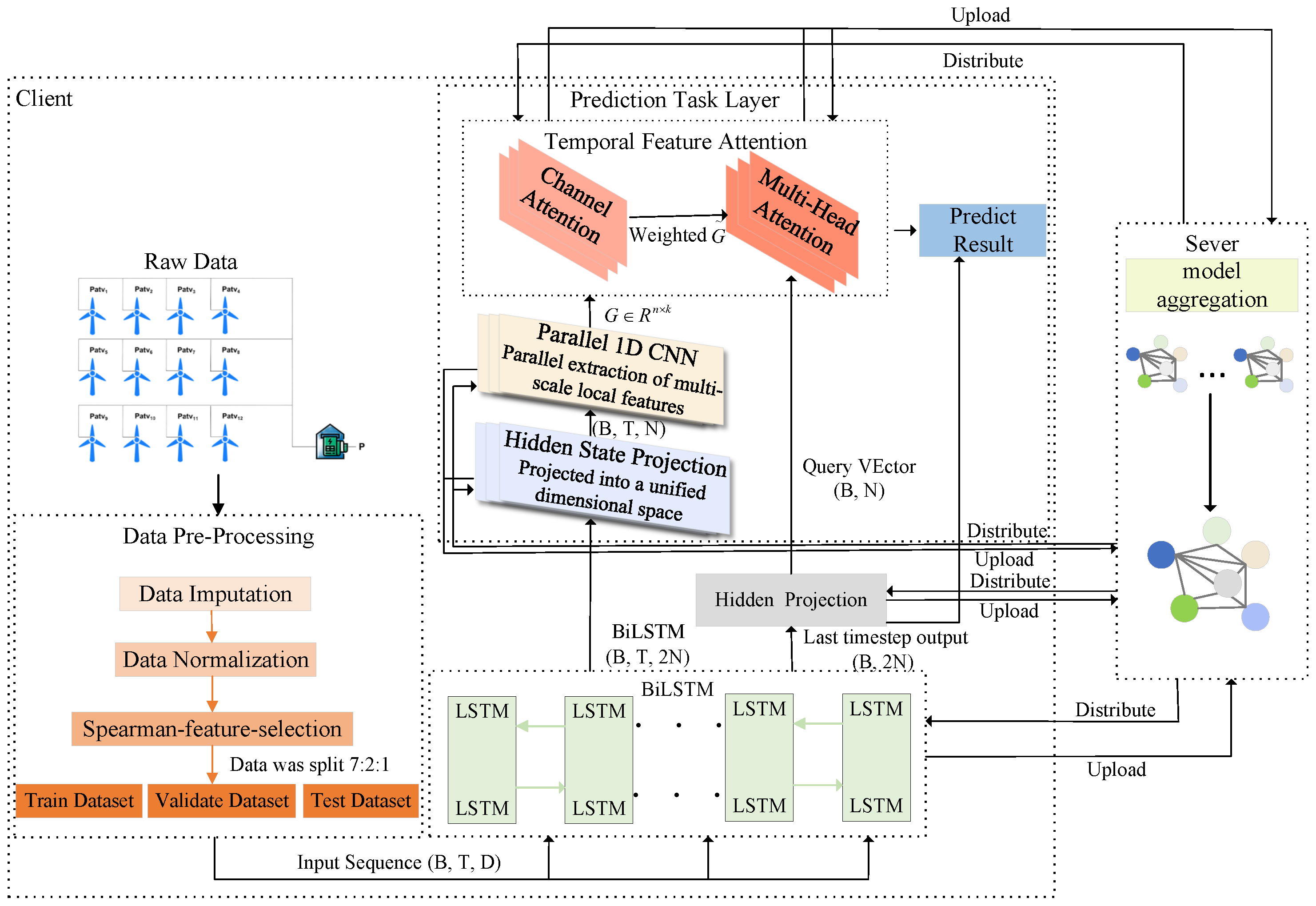
Considering the highly nonlinear, time-varying nature of wind power output with multiple meteorological factors and the existence of data distribution differences, this paper constructs a BiLSTM model integrating parallel 1D convolution and attention mechanism under the federated learning framework for multi-site wind power forecasting. The overall framework is shown in Figure 1. The main steps are as follows:

• Step 1: Multi-Site Multi-Variable Data Collection

Multi-variable time-series data such as wind speed, wind direction, air pressure, temperature, air density, and historical wind power are collected at multiple wind farms separately. All raw data is stored locally and not uploaded to the central server to meet data privacy and security requirements.

• Step 2: Local Data Preprocessing and Feature Selection

Each client locally preprocesses data (imputes missing values, removes outliers), screens power-correlated features via Spearman’s coefficients to eliminate redundancy, normalizes retained features, constructs single-step prediction samples with a sliding window (past period as input, next-step power as output), and splits them into local train/validation/test sets.

• Step 3: Construction of the Fed-AMHA (Federated Adaptive Multi-Head Attention) Model Architecture

First, BiLSTM extracts contextual hidden state sequences via bidirectional temporal modeling of input sequences; linear projection and parallel 1D-CNN are then applied to capture multi-scale local temporal features through kernel sliding, and channel attention plus adaptive multi-head temporal feature attention are stacked to weight time segments/feature channels; by synergistically enhancing critical information strongly correlated with the prediction target across both feature and temporal dimensions, the accuracy of feature representation in heterogeneous environments is significantly improved.

• Step 4: Federated Training of Model Parameters

Each client updates model parameters locally with the Adam optimizer, uploading only parameters/gradients to the central server; the server aggregates the parameters using FedAvg to get the global model and distributes it back for further local training. Multiple “local training–central aggregation” iterations achieve collaborative model optimization via multi-site information with no raw data sharing.

• Step 5: Model Inference and Performance Evaluation

After training converges, the global model is deployed on each wind farm client. Historical time window data from the local test set is input to output the wind power forecast for the next time step. Multiple error metrics are used to evaluate and compare the prediction accuracy and stability.

4.1. Feature Selection Based on Spearman’s Correlation Coefficient

Feature selection is a critical preliminary step in high-dimensional data modeling, with the core goal of eliminating irrelevant and redundant features and retaining a subset of features strongly correlated with the target variable. This reduces the computational complexity of the model, alleviates the curse of dimensionality, and simultaneously improves the model’s generalization ability. This paper adopts a filter-based Top-K feature selection method utilizing Spearman’s rank correlation. Compared to the classical Pearson Correlation Coefficient, Spearman rank correlation does not require the data to follow a normal distribution and can effectively capture nonlinear monotonic relationships between variables. This provides a stronger representational capability for wind power data, which is influenced by complex meteorological factors and exhibits highly nonlinear characteristics. Furthermore, since deep-sea offshore wind power data frequently contains outliers due to extreme weather disturbances, the Spearman method—which calculates based on ranks rather than raw values—demonstrates significant robustness to anomalies. The method adopted in this paper is a model-agnostic strategy, which can also meet the requirement of feature subspace consistency in multi-site federated learning or multi-source data scenarios.

Suppose the original dataset contains n time steps of data and d features, denoted by the feature matrix $A\in {\mathbb{R}}^{n\times d}$, where each row corresponds to a sample and each column corresponds to a candidate feature. The target variable is $y\in {\mathbb{R}}^n$, representing the prediction label of the samples. For each feature column $a_j$ ($j=1,2,\dots ,d$) in A, the Spearman rank correlation coefficient ${\rho }_j$ between the d features and y is calculated. The absolute value $|{\rho }_j|$ measures the correlation strength between the feature and the target variable. The value of $|{\rho }_j|$ is in the range of $[0,1]$, where a larger value indicates a higher degree of monotonic correlation between feature $a_j$ and target variable y, meaning the feature has stronger explanatory power and predictive contribution to the target variable.

Subsequently, all d candidate features are sorted in descending order of $|{\rho }_j|$, and the top K-ranked features are selected to form the final feature subset L. This selection process serves as an independent preprocessing step before data enters the downstream model, completely decoupled from subsequent modeling algorithms. It avoids introducing hyperparameter dependencies from downstream models and quickly reduces feature dimensions before modeling, significantly improving the efficiency of the overall modeling workflow.

$R\left(a_j\right)={[R\left(a_{j_1}\right),R\left(a_{j_2}\right),\dots ,R\left(a_{j_n}\right)]}^T$ denote the rank sequence of the feature column $a_j={(a_{j_1},a_{j_2},\dots ,a_{j_n})}^T$, where $R\left(a_{j_i}\right)$ represents the ascending rank of the feature value $a_{j_i}$ at the i-th time step among all observations in feature column $a_j$. The sample with the smallest feature value has a rank of 1, and the sample with the largest feature value has a rank of n. Similarly, let $R\left(y\right)={[R\left(y_1\right),R\left(y_2\right),\dots ,R\left(y_n\right)]}^T$ denote the rank sequence of the target variable y, following the same rank transformation rules as the feature columns.

Based on the rank-transformed sequences, the Spearman rank correlation coefficient ${\rho }_j$ for the j-th feature column is calculated as

$${\rho }_j=\mathrm{corr}\left(R\left(x_j\right),R\left(y\right)\right)={\displaystyle \frac{\mathrm{cov}\left(R\left(x_j\right),R\left(y\right)\right)}{{\sigma }_{R\left(x_j\right)}·{\sigma }_{R\left(y\right)}}}$$

(6)

where $\mathrm{cov}(·,·)$ denotes the covariance, and $\sigma$ denotes the standard deviation.

After calculating the Spearman rank correlation coefficients between all features and the target variable, we obtain the set of correlation coefficients ${\left\{{\rho }_j\right\}}_{j=1}^d$. These coefficients are then sorted in descending order of $|{\rho }_j|$, and the indices of the top k feature columns are selected to construct the feature subset L. Finally, we extract the columns from the original input matrix $A\in {\mathbb{R}}^{n\times d}$ whose indices belong to L, yielding the filtered input matrix $A_L$ as the input to the subsequent prediction model. This retains the k features most strongly correlated with the target variable, thereby improving model performance and generalization ability.

4.2. Sequence Feature Encoding Network Based on BiLSTM

The Bidirectional Long Short-Term Memory (BiLSTM) network introduces a bidirectional recursive structure on the basis of the standard LSTM. By simultaneously constructing forward and backward information flows, it jointly models the forward and backward dependencies of the sequence. In wind power forecasting tasks, meteorological variables and power output exhibit significant temporal correlation and nonlinear coupling characteristics; unidirectional LSTM models often struggle to simultaneously account for historical evolutionary trends and current local abrupt variations. In contrast, BiLSTM can concurrently extract the cumulative effects and evolutionary trends of observation sequences, providing higher-quality temporal representations for subsequent modules. Compared to purely attention-based Transformer models, BiLSTM, leveraging its gating mechanism, exhibits superior robustness when capturing wind power data characterized by strict temporal causality and physical continuity, effectively mitigating overfitting issues in high-noise environments. A BiLSTM unit consists of a forget gate, an input gate, and an output gate, with its internal state update process as follows:

Forget Gate:

$$f_t=\sigma \left(w_f·\left[h_{t-1},x_t\right]+b_f\right)$$

(7)

Input Gate:

$$i_t=\sigma \left(w_i·\left[h_{t-1},x_t\right]+b_i\right)$$

(8)

Candidate Memory Cell:

$${\tilde{C}}_t=\tanh \left(w_c·\left[h_{t-1},x_t\right]+b_c\right)$$

(9)

Output Gate:

$$o_t=\sigma \left(w_o·\left[h_{t-1},x_t\right]+b_o\right)$$

(10)

Long-Term Memory State Update:

$$C_t=f_t·C_{t-1}+i_t·{\tilde{C}}_t$$

(11)

Short-Term Memory (Hidden State) Output:

$$h_t=o_t·\tanh \left(C_t\right)$$

(12)

where $\sigma (·)$ denotes the Sigmoid activation function, $\tanh (·)$ denotes the hyperbolic tangent function; $x_t$ is the input feature vector at time step t; $h_{t-1}$ represents the hidden state from the previous time step; $b_f,b_i,b_c,b_o$ are the bias terms for the forget gate, input gate, candidate memory cell, and output gate, respectively; $w_f,w_i,w_c,w_o$ denote the weight matrices for the corresponding gate structures.

In wind power forecasting, the BiLSTM network is used to perform temporal modeling on multi-variable time-series features. After the historical meteorological feature sequence is input, the forget gate calculates a probability value $f_t$ to retain key information from the long-term memory $C_{t-1}$ of the previous time step. The input gate generates a probability value $i_t$ to filter the current candidate features ${\tilde{C}}_t$, which are then weighted and fused with historical information to obtain the new long-term memory $C_t$. The output gate then generates $o_t$ based on the current input and historical state, filtering $C_t$ to extract core information and outputting the short-term memory $h_t$. This state comprehensively reflects the temporal features related to wind power. By jointly modeling with forward and backward LSTMs, BiLSTM can fully exploit the bidirectional temporal dependencies in the data, extracting effective temporal features and providing high-quality representations for subsequent attention modules.

4.3. Temporal Feature Extraction Parallel Sublayer

Although BiLSTM can effectively encode the global and bidirectional dependencies of sequences, its hidden state sequence still contains a large number of local dynamic patterns (e.g., short-term wind speed spikes, local oscillations), which make important contributions to wind power forecasting. To further exploit the local temporal dynamic features embedded in the BiLSTM hidden states, this paper introduces a parallel 1D convolutional neural network sublayer after the sequence encoder. Compared to traditional serial convolution, this parallel design enables the model to independently capture heterogeneous physical evolutionary patterns across different variable branches, thereby preserving the site-specific wind characteristic responses within the federated global model. This sublayer consists of multiple groups of independent 1D convolution kernels, which perform convolution operations on the hidden state sequence along the temporal dimension to effectively extract multi-scale temporal features. Let the hidden state matrix of BiLSTM within the time window $[t,t+p-1]$ be expressed as

$$H=\left[\begin{array}{cccc}{h}_{t,1}& h_{t,2}& \cdots & h_{t,n}\\ h_{t+1,1}& h_{t+1,2}& \cdots & h_{t+1,n}\\ ⋮& ⋮& \ddots & ⋮\\ h_{t+p-1,1}& h_{t+p-1,2}& \cdots & h_{t+p-1,n}\end{array}\right]\in {\mathbb{R}}^{p\times n}$$

(13)

where n denotes the feature dimension, p denotes the time window length, and the r-th column of matrix $h_{t,r}$ corresponds to the hidden state sequence of the r-th feature over p consecutive time steps.

We utilize the output of the BiLSTM at the last time step as the query vector. Assuming a window length of T, with the forward LSTM output at time step T being ${\overrightarrow{h}}_T$ and the backward LSTM output at time step 1 being ${\overrightarrow{h}}_1$, the bidirectional concatenation at the final time step is denoted as $h_T=[{\overrightarrow{h}}_T;{\overrightarrow{h}}_1]$. Therefore, the query vector is defined as

$$h_{\mathrm{last}}=W_q{h}_T+b_q\in {\mathbb{R}}^n$$

(14)

where $W_a,b_q$ denotes a learnable parameter. Vector $h_{last}$ encapsulates the overall temporal information of the sequence and serves as the query for evaluating the correlation of features in subsequent branches.

The parallel 1D-CNN sublayer consists of k 1D convolution kernels. For ease of expression, the convolution kernel matrix is defined as

$$C=[c_1,c_2,\dots ,c_k]=\left[\begin{array}{cccc}{c}_{1,1}& c_{1,2}& \cdots & c_{1,p}\\ c_{2,1}& c_{2,2}& \cdots & c_{2,p}\\ ⋮& ⋮& \ddots & ⋮\\ c_{k,1}& c_{k,2}& \cdots & c_{k,p}\end{array}\right]\in {\mathbb{R}}^{k\times p}$$

(15)

where $c_j={[c_{j,1},c_{j,2},\dots ,c_{j,p}]}^T\in {\mathbb{R}}^p$ denotes the j-th 1D convolution kernel.

After the convolution operation, the convolution results of k feature dimensions are combined to obtain the overall output matrix of the parallel 1D-CNN sublayer:

$$G=CH=\left[\begin{array}{cccc}{g}_{1,1}& g_{1,2}& \cdots & g_{1,k}\\ g_{2,1}& g_{2,2}& \cdots & g_{2,k}\\ ⋮& ⋮& \ddots & ⋮\\ g_{n,1}& g_{n,2}& \cdots & g_{n,k}\end{array}\right]\in {\mathbb{R}}^{k\times n}$$

(16)

It can be seen that each element of matrix G represents a hierarchical temporal feature extracted from the time window by different convolution kernels under the same feature dimension. Since these features are obtained by convolution operations on the BiLSTM hidden states over consecutive time steps, they can effectively characterize the local temporal evolution patterns in the hidden state sequence. In this sense, the parallel 1D-CNN sublayer achieves further extraction and enhancement of temporal features in the BiLSTM hidden states, providing richer temporal feature representations for subsequent attention mechanisms.

4.4. Feature Enhancement Module with Dual-Dimensional Attention Mechanism

After the BiLSTM temporal encoder and parallel 1D-CNN sublayer, the model extracts multi-scale temporal features and local pattern information. However, there are significant differences in the contribution of different feature channels and the value of historical information at different time steps. To address this, this section introduces a dual-dimensional attention mechanism, which performs adaptive weighting from the feature channel and temporal dimensions to enhance key information, suppress redundant noise, and improve the discriminability and accuracy of feature representations.

Let the fused feature representation after BiLSTM and parallel 1D-CNN be

$$G\in {\mathbb{R}}^{k\times n}$$

(17)

where n denotes the feature dimension (corresponding to the number of parallel branches), and k denotes the number of convolution output channels. The channel attention mechanism first extracts the overall response features of each channel through a global information aggregation operation. Specifically, global average pooling along the temporal dimension is used to generate a channel description vector:

$$z=[z_1,z_2,\dots ,z_k]\in {\mathbb{R}}^k$$

(18)

where $z_k={\displaystyle \frac{1}{n}}{\sum }_{r=1}^n{g}_{r,k}$.

Subsequently, a learnable channel mapping function is used to model channel importance, which can be expressed as

$$w_a=\sigma \left(w_{p}z+b_p\right)$$

(19)

where $w_p$ and $b_p$ are learnable parameters, $\sigma (·)$ denotes the Sigmoid activation function, and $w_a\in (0,1)$ is the attention weight for each channel.

Finally, the channel attention weights are reapplied to the original feature representation to achieve feature recalibration:

$$\tilde{G}=G\odot w_a$$

(20)

where ⊙ denotes element-wise multiplication along the channel dimension.

The feature sequence after processing by the channel attention mechanism is

$$\tilde{G}={\{{\tilde{g}}_1,{\tilde{g}}_2,\dots ,{\tilde{g}}_n\}}^T$$

(21)

where ${\tilde{g}}_i\in {\mathbb{R}}^k$. To extract the correlation information among branches from different subspaces, four independent attention heads are configured, the multi-head temporal attention mechanism characterizes temporal dependencies from different temporal perspectives by introducing multiple parallel attention subspaces. For the m-th attention head, its attention score function is defined as

$$e_i^m=h_{\mathrm{last}}^{\top }{W}^{mT}{\tilde{g}}_i$$

(22)

where $W^m\in R^{k\times n}$ is the learnable parameter for the m-th attention head. By explicitly introducing $h_{last}$, the model can dynamically adjust its attention to the features ${\tilde{g}}_i$ of each branch based on the final state representation of the entire sequence.

Subsequently, the attention scores along the temporal dimension are normalized using the Softmax function to obtain temporal attention weights:

$${\alpha }_i^m={\displaystyle \frac{\exp \left(e_i^m\right)}{{\sum }_{j=1}^n\exp \left(e_j^m\right)}},i=1,\dots ,n$$

(23)

Based on the temporal attention weights, the context feature vector of the m-th attention head can be expressed as

$$s^m={\displaystyle \sum _{i=1}^n}{\alpha }_i^m{\tilde{g}}_n,s^m\in {\mathbb{R}}^k$$

(24)

Unlike traditional direct fusion approaches, this paper employs an adaptive weighted fusion strategy for the outputs of multiple attention heads. Let $\pi \in {\mathbb{R}}^M$ denote the learnable log-odds representing the contribution of each head, which is a learnable parameter of the model. Then, the fusion weight ${\beta }_m$ for each head can be defined as

$${\beta }_m={\displaystyle \frac{\exp \left({\pi }_m\right)}{{\sum }_{m^{\prime }=1}^M\exp \left({\pi }_{m^{\prime }}\right)}}$$

(25)

where M denotes the total number of heads, and ${\pi }_m$ represents the original importance score of the m-th attention head. After applying the fusion weights ${\beta }_m$, the final fused features are obtained as follows:

$$S=W_o\left(\mathrm{Concat}(s^1,\dots ,s^M)\beta \right),W_o\in {\mathbb{R}}^{M\times k}$$

(26)

where M denotes the number of attention heads, and $w_o$ is the output projection matrix.

This adaptive multi-head temporal attention mechanism can model historical features from multiple temporal perspectives, enabling the model to not only focus on single critical time points but also assign reasonable weights to different time segments based on the temporal characteristics of wind power changes. As a result, the model can more effectively capture both short-term and long-term temporal dependencies, improving the accuracy and stability of wind power forecasting under complex meteorological conditions.

4.5. Feature Fusion and Prediction

The task query vector $h_{last}$ and the context feature S are fused in the same intermediate representation space:

$$z=w_1{h}_{last}+w_{2}S+b_1$$

(27)

$$\widehat{y}=w_{3}z+b_2$$

(28)

where $w_1\in {\mathbb{R}}^{n\times r}$, $w_2\in {\mathbb{R}}^{k\times r}$, $b_1\in {\mathbb{R}}^r$, $b_2\in \mathbb{R}$ are responsible for mapping the two types of information to the r-dimensional fusion space; $w_3\in {\mathbb{R}}^{r\times 1}$ is the output projection matrix, $z\in {\mathbb{R}}^{B\times r}$ is the fused feature, and $\widehat{y}\in {\mathbb{R}}^{B\times 1}$ is the final wind power prediction value.

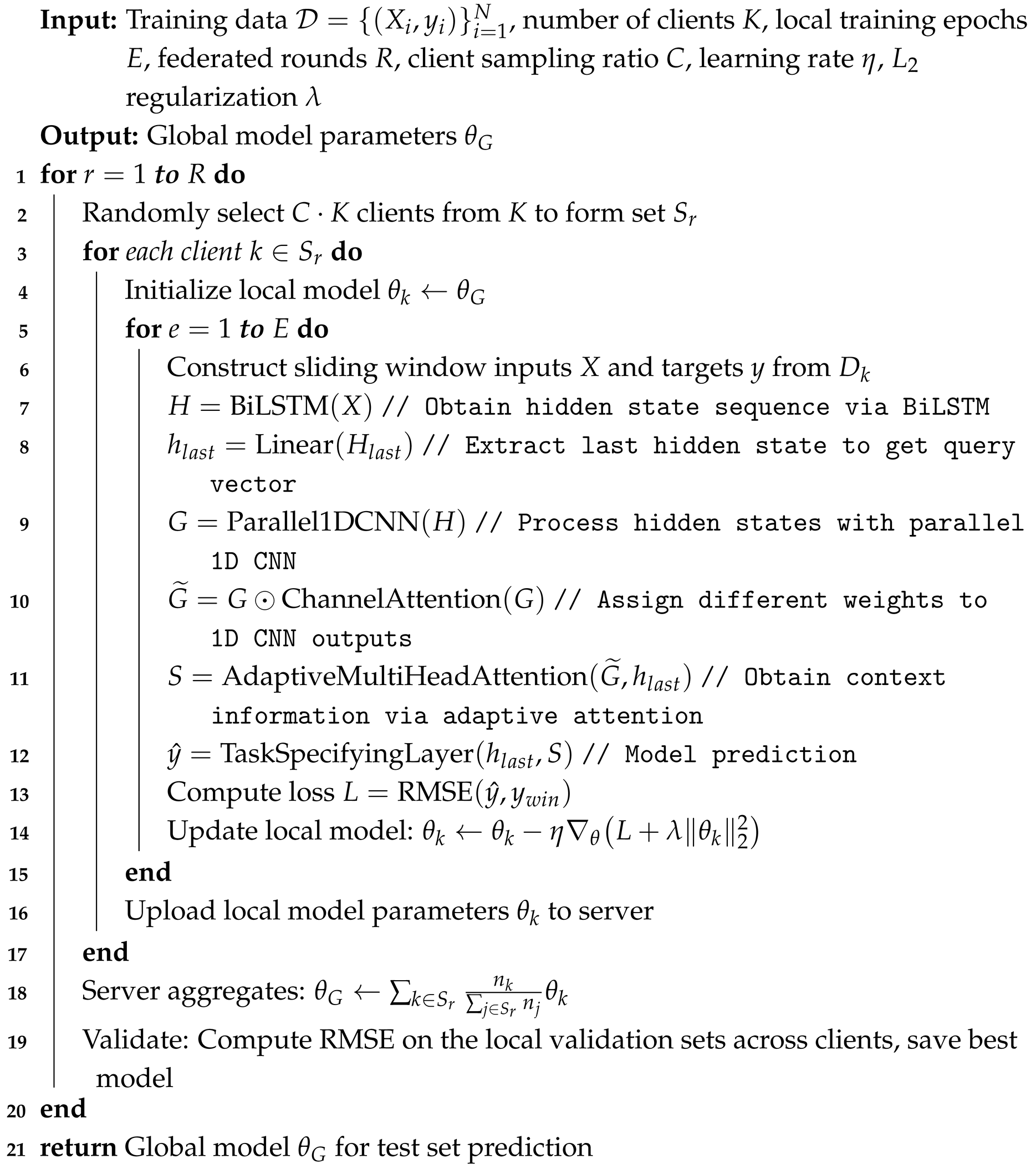
This prediction structure can simultaneously utilize the global temporal representation $h_{last}$ encoded by BiLSTM and the local critical pattern information S filtered by the attention mechanism, thereby improving the accuracy and stability of wind power forecasting under complex meteorological conditions. The algorithm is as shown in Algorithm 1.

Algorithm 1: Fed-AMHA Algorithm

5. Experimental Section

5.1. Experimental Setup

The experiments in this study were implemented using the Python 3.9.12 and PyTorch 2.0.0 frameworks on the Windows 11 operating system, with computations performed on a system equipped with an NVIDIA A40 GPU (NVIDIA Corporation, Santa Clara, CA, USA). The model hyperparameters are configured as follows: each sample utilizes 24 historical time steps as input. In our experiments, the data is partitioned into 8 clients based on the number of stations. The number of local training epochs is set to 5, while the number of federal communication rounds is 120. We perform random client sampling with a sampling rate of 0.5. For federated aggregation, the FedAvg algorithm is employed. The batch size is set to 64, and the learning rate is 0.001. In the multi-scale CNN module, a parallel convolutional structure is employed, featuring three convolutional layers with kernel sizes of [3, 5, 7]. Each scale outputs 16 feature channels, which are processed via Batch Normalization and ReLU activation functions; temporal features are subsequently extracted through average pooling. For the BiLSTM network, three stacked layers are utilized, with each layer containing 64 hidden units and a dropout rate of 0.3 to prevent overfitting; the LSTM outputs are then processed using LayerNorm. In the attention mechanism component, a 4-head self-attention module with an attention dimension of 48 is adopted to capture spatiotemporal features. Within the task-specific layer, a linear fusion mechanism is used to adaptively fuse the LSTM and CNN features, with the final prediction generated through a fully connected layer incorporating a 0.2 dropout rate.

5.2. Dataset Description

To verify the effectiveness and robustness of the proposed method, next-step wind power forecasting experiments are conducted on two representative datasets: the FuJian dataset and the Baidu KDD Cup 2022 dataset. Detailed specifications of these datasets are summarized in

Table 2. All features included in the Fujian dataset.

No.	Column Name	Description
1	Station ID	Unique identifier for the wind farm station.
2	Time	Timestamp of the data record.
3	Air Pressure	Atmospheric pressure (Pa).
4	Rel. Humidity	Percentage of water vapor relative to saturation (%).
5	Cloud Cover	Proportion of sky covered by clouds.
6	10 m Wind Speed	Wind speed at 10 m height (m/s).
7	10 m Wind Dir.	Wind direction at 10 m height (°).
8	Temp.	Air temperature (K).
9	Irradiance	Solar radiation energy per unit area (J/m2).
10	Precipitation	Amount in meters (m). Note: 1 m = 1000 mm.
11	100 m Wind Speed	Wind speed at 100 m height (m/s).
12	100 m Wind Dir.	Wind direction at 100 m height (°).
13	Power Output	Actual power output of units (MW).

and

Table 3. All features included in the KDD Cup dataset.

No.	Feature	Description
1	TurbID	Wind turbine ID.
2	Day	Day of the record.
3	Tmstamp	Created time of the record.
4	Wspd	Wind speed recorded by the anemometer.
5	wdir	Angle between wind direction and turbine nacelle position.
6	Etmp	Temperature of the surrounding environment.
7	Itmp	Temperature inside the turbine nacelle.
8	Ndir	Nacelle direction (yaw angle of the nacelle).
9	Pabl1	Pitch angle of blade 1.
10	Pabl2	Pitch angle of blade 2.
11	Pabl3	Pitch angle of blade 3.
12	Prtv	Reactive power.
13	Patv	Active power (target variable).

. The FuJian dataset comprises multivariate time-series data from five wind power plants in Fujian, China. Recorded at 15 min intervals from 3 January 2022to 30 April 2023, it incorporates meteorological features such as wind speed, wind direction, and atmospheric pressure. TheKDD Cup 2022 dataset, obtained from a wind farm’s SCADA system, features a 10 min sampling interval and covers 245 days of operational records across 134 turbines. This dataset provides a comprehensive feature set including environmental variables (wind speed, wind direction, and external temperature) as well as turbine-specific operational indicators (blade angle and internal temperature).

For the FuJian dataset, rows are removed if the values in the feature or target columns are zero, or if the target column values are less than zero. Regarding the KDD Cup dataset, following the methodology described by Zhou et al. [33], we eliminate outliers and missing values before applying MinMaxScaler for normalization. During feature selection, the Top-K value is set to 6 for the FuJian dataset and 4 for the KDD Cup dataset. Due to discrepancies in geographical locations and turbine configurations, the datasets exhibit significant non-independent and identically distributed (non-IID) characteristics. In compliance with temporal causality, the data are partitioned chronologically into training, validation, and testing sets with a ratio of 7:2:1. Furthermore, each station or turbine is designated as an individual client. This setup serves to authentically simulate the non-IID data distribution in federated learning scenarios, thereby enhancing parallel training efficiency and strengthening the model’s generalization capabilities.

5.3. Evaluation Metrics

Error evaluation metrics are commonly used to assess prediction performance independently of data size [31,32]. In this study, MAE, RMSE, MSE, NRMSE, and $R^2$ score are employed to evaluate the predictive accuracy of the models. The formulas for these evaluation metrics are as follows:

• MSE (Mean Squared Error): Measures the quadratic loss of prediction errors; lower values indicate better performance.

  $$MSE={\displaystyle \frac{1}{N}}{\displaystyle \sum _{i=1}^N}{(y_i-{\widehat{y}}_i)}^2$$

  (29)
• RMSE (Root Mean Squared Error): The square root of MSE, providing an intuitive reflection of the average error magnitude.

  $$RMSE=\sqrt{MSE}=\sqrt{{\displaystyle \frac{1}{N}}\sum _{i=1}^N{(y_i-{\widehat{y}}_i)}^2}$$

  (30)
• NRMSE (Normalized RMSE): By normalizing RMSE to the actual range of the target variable, this metric eliminates scale effects, facilitating comparisons between models across different datasets or scales:

  $$NRMSE={\displaystyle \frac{RMSE}{\max \left(y\right)-\min \left(y\right)}}$$

  (31)
• MAE (Mean Absolute Error): Measures the average absolute deviation between predicted and ground-truth values; it offers better robustness against outliers compared to MSE and RMSE:

  $$MAE={\displaystyle \frac{1}{N}}{\displaystyle \sum _{i=1}^N}|y_i-{\widehat{y}}_i|$$

  (32)
• $R^2$ (Coefficient of Determination): Represents the proportion of variance in the target variable explained by the model. Values closer to 1 indicate higher accuracy; a negative value suggests that the model’s predictive capability is inferior to a baseline model that simply uses the target mean:

  $$R^2=1-{\displaystyle \frac{{\sum }_i{(y_i-{\widehat{y}}_i)}^2}{{\sum }_i{(y_i-\overline{y})}^2}}$$

  (33)

  where $\overline{y}={\displaystyle \frac{1}{N}}{\sum }_i{y}_i$.

5.4. Baseline

The experiments are conducted using the LSTM model as the primary baseline. The core objective of this study is to compare the proposed method with several other state-of-the-art wind power forecasting models to demonstrate its superior error reduction capabilities. We compare the proposed method with several other wind power forecasting approaches, including SABO, MTTFA, LSTM, DSCBN, FedWindT, and PEL. Although methods such as SABO, MTTFA, LSTM, and DSCBN were originally proposed for centralized scenarios, they are integrated into a federated framework in this study—utilizing the same client partitioning, communication rounds, and local training configurations—to ensure a fair comparison with Fed-AMHA. The details are as follows:

• MTTFA [26]: This model integrates Long Short-Term Memory (LSTM), Convolutional Neural Networks (CNNs), and an attention mechanism. It utilizes a hierarchical structure consisting of task-sharing and task-specific layers to enhance forecasting accuracy.
• SABO [27]: The SABO model reconstructs data into a three-dimensional “Time–Space–Feature” structure. It employs 3D-CNN for spatiotemporal feature extraction and dimensionality reduction, utilizes BiLSTM to capture bidirectional temporal dependencies, and leverages an attention mechanism to focus on key features before outputting predictions through a fully connected layer.
• DSGBN [34]: By combining federated learning with the Transformer model, this method leverages the self-attention mechanism of Transformers to capture long-term dependencies and complex interactions in time-series data. The approach aims to enhance wind power forecasting accuracy while ensuring data privacy protection.
• FedWindT [35]: DSGBN is designed to improve the accuracy of renewable energy forecasting by combining Graph Convolutional Networks (GCNs) and Bidirectional Long Short-Term Memory (BiLSTM). The proposed dual-stream network captures spatial dependencies via GCNs and temporal dependencies via BiLSTM, effectively enhancing overall predictive performance.
• PEL [36]: This method utilizes a dual-stream network architecture that integrates a general network with a personalized network. The general network is designed to extract global shared features, while the personalized network is tailored to the specific data characteristics of each turbine, thereby effectively improving overall prediction performance.

5.5. Experimental Results and Analysis

5.5.1. Performance Analysis of Different Models Across All Datasets

Table 4. Performance comparison across datasets (The experimental results for the KDD Cup dataset are presented in percentages).

Dataset	Model	MSE	RMSE	NRMSE	MAE	R2
FuJian	SABO	3.685	1.919	0.0436	1.198	0.950
	MTTFA	3.631	1.905	0.0433	1.152	0.950
	LSTM	3.774	1.942	0.0441	1.207	0.948
	DSCBN	3.866	1.966	0.0446	1.328	0.947
	FedWindT	3.692	1.921	0.0436	1.140	0.949
	PEL	4.255	2.062	0.0468	1.425	0.941
	Fed-AMHA	3.621	1.903	0.0432	1.144	0.951
KDD Cup	SABO	0.784	8.858	8.8594	6.150	92.976
	MTTFA	0.881	9.387	9.3873	6.636	92.096
	LSTM	0.795	8.918	8.9193	6.209	92.864
	DSCBN	0.819	9.051	9.0510	6.474	92.651
	FedWindT	0.797	8.928	8.9299	5.851	92.908
	PEL	0.881	9.384	9.3856	6.579	92.488
	Fed-AMHA	0.747	8.648	8.6492	5.851	93.090

Note: Boldface indicates the optimal performance, and underline indicates the suboptimal performance.

presents the experimental results for various models across different datasets. For the KDD Cup dataset, the metrics are displayed as percentages. Experimental results demonstrate that the proposed Fed-AMHA model achieves state-of-the-art performance across most metrics on both datasets, highlighting its superiority and robustness in wind power forecasting tasks. As shown in Table 4, for the FuJian dataset, Fed-AMHA reduces the MSE by 0.010 compared to the runner-up MTTFA (a relative improvement of 0.28%) and outperforms LSTM, DSCBN, and PEL, with MSE reductions of 4.0%, 6.3%, and 14.9%, respectively. It achieves an $R^2$ of 0.951, indicating the best fitting effect. Although its MAE is slightly higher than that of the FedWindT model, Fed-AMHA outperforms FedWindT in the remaining four metrics, exhibiting a more concentrated error distribution. For the KDD CUP dataset, Fed-AMHA reduces the MSE by 4.7% compared to SABO, 6.0% compared to LSTM, 6.3% compared to FedWindT, and 15.2% compared to PEL. It similarly achieves the highest $R^2$ score. While its MAE ties with FedWindT for the best performance, our RMSE and NRMSE are significantly smaller, suggesting a stronger penalty for large errors and more stable predictions. Cross-comparisons indicate that Fed-AMHA maintains stable performance across two distinct datasets. In contrast, traditional LSTM shows limitations in handling non-stationary features, while DSCBN and MTTFA exhibit performance fluctuations across different scenarios. The strong performance of FedWindT on the FuJian dataset underscores the competitiveness of Transformer backbones in wind power forecasting. The relatively higher error metrics for PEL on the FuJian dataset may be attributed to its personalized branch structure or specific meteorological and geographical factors.

In summary, the proposed Fed-AMHA model—through the deep coupling of BiLSTM and parallel 1D-CNN—achieves precise representation of global bidirectional temporal dependencies and variable-level local evolutionary patterns. Furthermore, by utilizing a query-guided adaptive multi-head attention mechanism to dynamically calibrate feature weights, the model effectively addresses the challenges of data heterogeneity in federated learning, significantly enhancing the accuracy and stability of offshore wind power forecasting.

5.5.2. Significance Test

To further validate the statistical significance of the performance improvements achieved by the Fed-AMHA model, this study employs the Diebold–Mariano (DM) test for pairwise comparative analysis between Fed-AMHA and various baseline models. First, we define the loss differential at each prediction time step as $d_t=L\left(e_{i,t}\right)-L\left(e_{Fed-AMHA,t}\right)$, where L represents the squared error loss, and $e_{i,t}$ and $e_{Fed-AMHA,t}$ denote the prediction errors of the baseline model and the proposed model, respectively.

The null hypothesis ($H_0$) of the DM test assumes no significant difference in prediction accuracy between the two models, i.e., $E\left[d_t\right]=0$, while the alternative hypothesis ($H_1$) is $E\left[d_t\right]\ne 0$. The DM test statistic is calculated as $DM={\displaystyle \frac{\overline{d}}{\sqrt{{\widehat{\sigma }}_{\overline{d}}^2}}}$, where $\overline{d}$ is the sample mean of the loss differential and ${\widehat{\sigma }}_{\overline{d}}^2$ is the estimated variance. The corresponding p-value is calculated as $P=2[1-\mathsf{\Phi }(\left|DM\right|\left)\right]$, where $\mathsf{\Phi }(·)$ denotes the cumulative distribution function of the standard normal distribution. When $DM>0$ and $p<0.05$, the null hypothesis is rejected, indicating that Fed-AMHA is statistically superior to the corresponding baseline.

Table 5. Statistical results of significance test (DM test).

Dataset	Comparison Model	Mean (${\mathit{d}}_{\mathit{t}}$)	DM	p
FuJian	Fed-AMHA vs. SABO	0.00036	6.24749	$4.17098631{\times 10}^{-10}$
	Fed-AMHA vs. MTTFA	0.00133	20.99548	$7.21306563{\times 10}^{-98}$
	Fed-AMHA vs. LSTM	0.00047	18.73892	$2.38403860{\times 10}^{-78}$
	Fed-AMHA vs. DSCBN	0.00071	23.85328	$9.36135009{\times 10}^{-126}$
	Fed-AMHA vs. FedWindT	0.00011	2.59188	0.00954
	Fed-AMHA vs. PEL	0.00094	12.31343	$7.66893231{\times 10}^{-35}$
KDD CUP	Fed-AMHA vs. SABO	0.06372	1.08241	0.27906
	Fed-AMHA vs. MTTFA	0.00992	0.47598	0.63408
	Fed-AMHA vs. LSTM	0.15297	6.61484	$7.66893231{\times 10}^{-35}$
	Fed-AMHA vs. DSCBN	0.24496	15.88629	$7.88545428{\times 10}^{-57}$
	Fed-AMHA vs. FedWindT	115.77778	32.67412	$3.64175915{\times 10}^{-234}$
	Fed-AMHA vs. PEL	104.63249	32.16333	$5.74923617{\times 10}^{-227}$

presents the DM test results for the FuJian and KDD Cup datasets. Overall, on the FuJian dataset, the $DM$ statistics for Fed-AMHA relative to all listed baselines are positive, and the two-sided p are all below the significance level of 0.05, demonstrating that the improvements are statistically significant. On the KDD Cup dataset, Fed-AMHA significantly outperforms LSTM, DSCBN, FedWindT, and PEL. However, the comparison with SABO and MTTFA failed to reject the null hypothesis at the 0.05 level, suggesting that under the current training settings for this specific dataset, there is no statistically significant difference between Fed-AMHA and these two strong baselines.

5.5.3. Visualization of Multi-Dimensional Performance

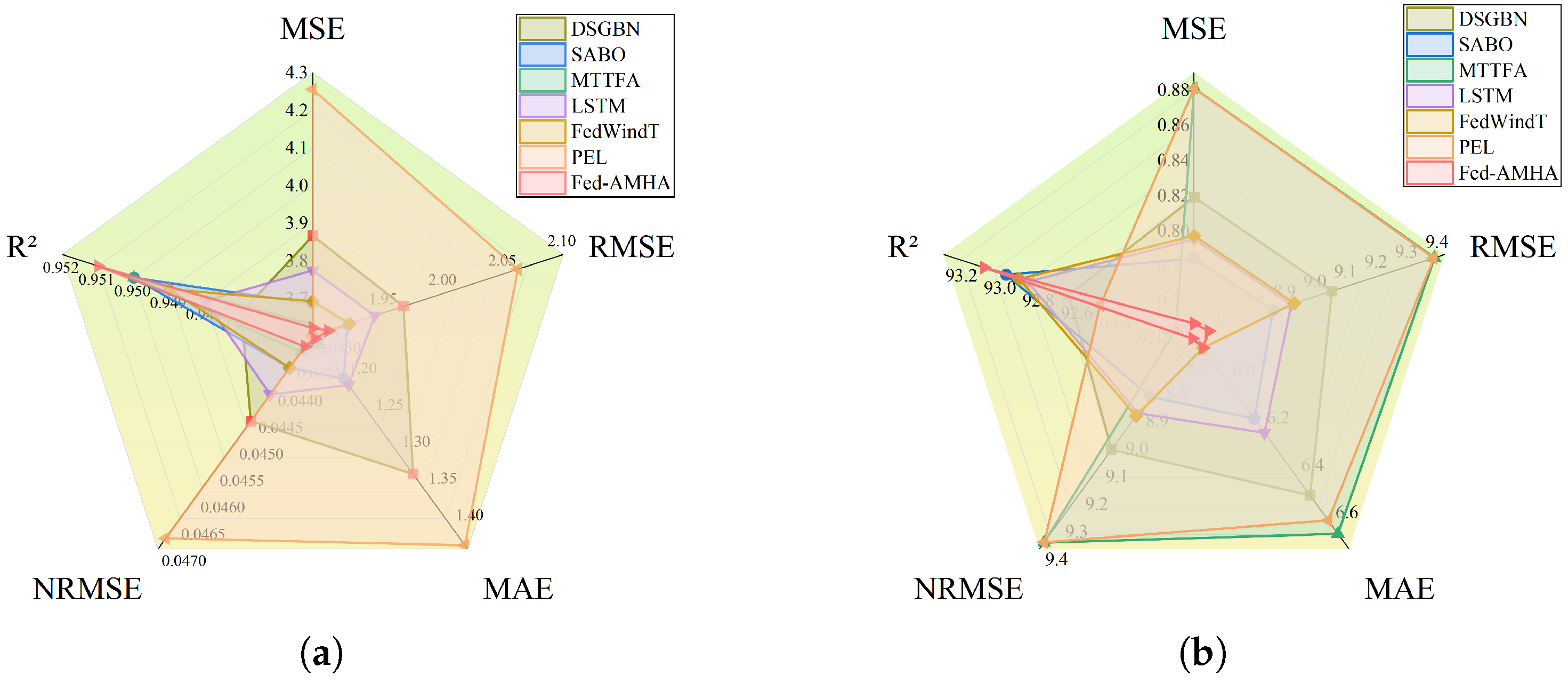
To facilitate a clearer observation of the experimental results, a visualization analysis was conducted to compare the performance of different models across various datasets, with the results illustrated in Figure 2. The radar charts of model performance visually illustrate that the proposed Fed-AMHA model exhibits a balanced and expansive “cone-shaped” structure across all evaluation metrics. In the error-related dimensions (MSE, RMSE, MAE, and NRMSE), the model consistently achieves either the optimal or suboptimal values across all metrics, while the $R^2$ metric shows a prominent outward protrusion. This profile reflects that Fed-AMHA achieves high prediction accuracy while possessing strong interpretability. Baseline models, such as PEL on the FuJian dataset and MTTFA on the KDD CUP dataset, exhibit a distinct concave characteristic, particularly with significant inward deviations in the $R^2$ direction. These irregularities reveal inherent limitations in their explanatory power and an imbalance in error control. Overall, the contrast in radar chart morphology underscores the superior stability and integration of Fed-AMHA. Its expansive and sharp profile confirms its robustness in multi-metric evaluations, ensuring better engineering applicability and reliability compared to the fluctuating performance of competing methods.

5.5.4. Results Analysis Under Different Sampling Scales on the FuJian Dataset

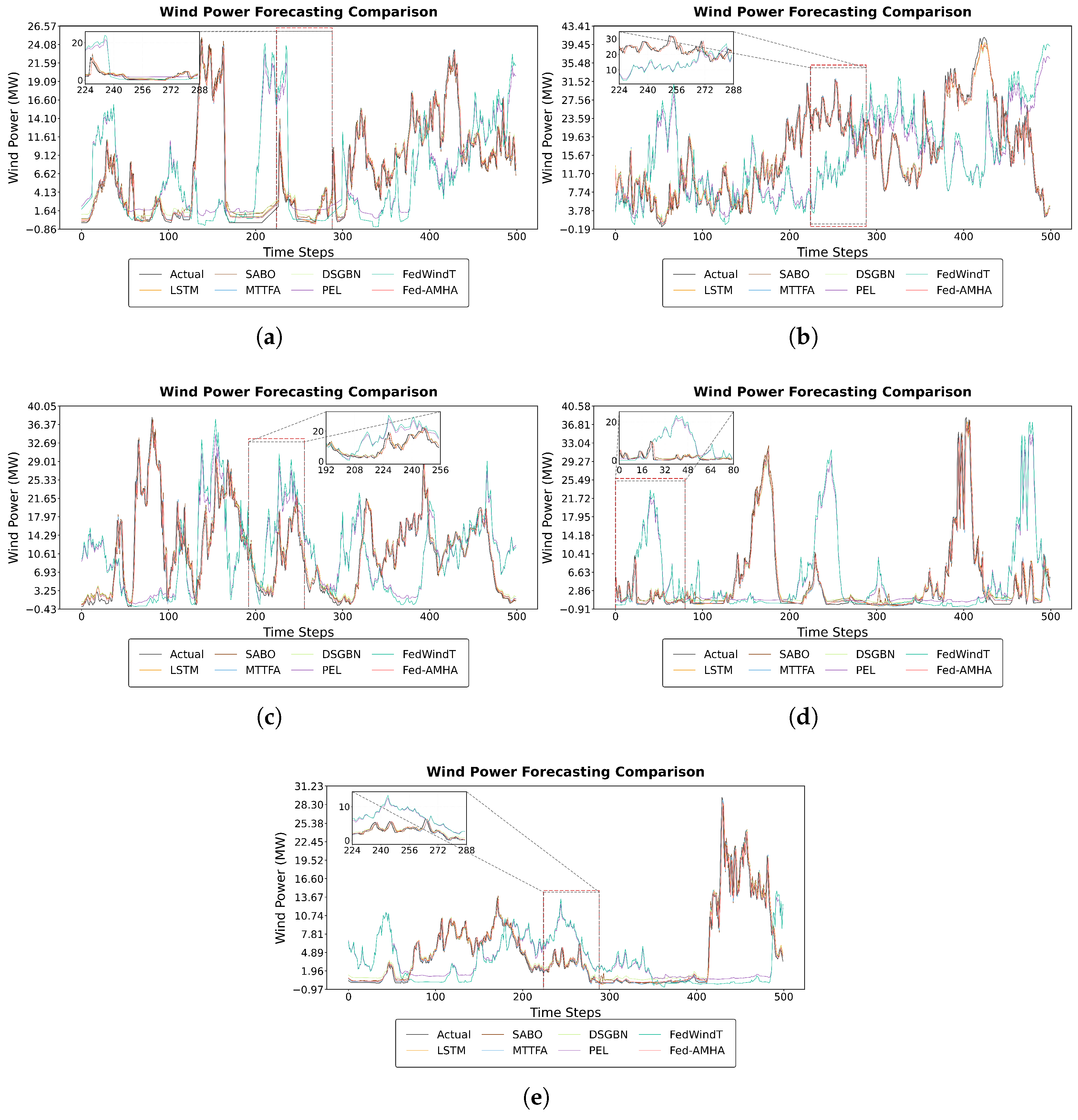
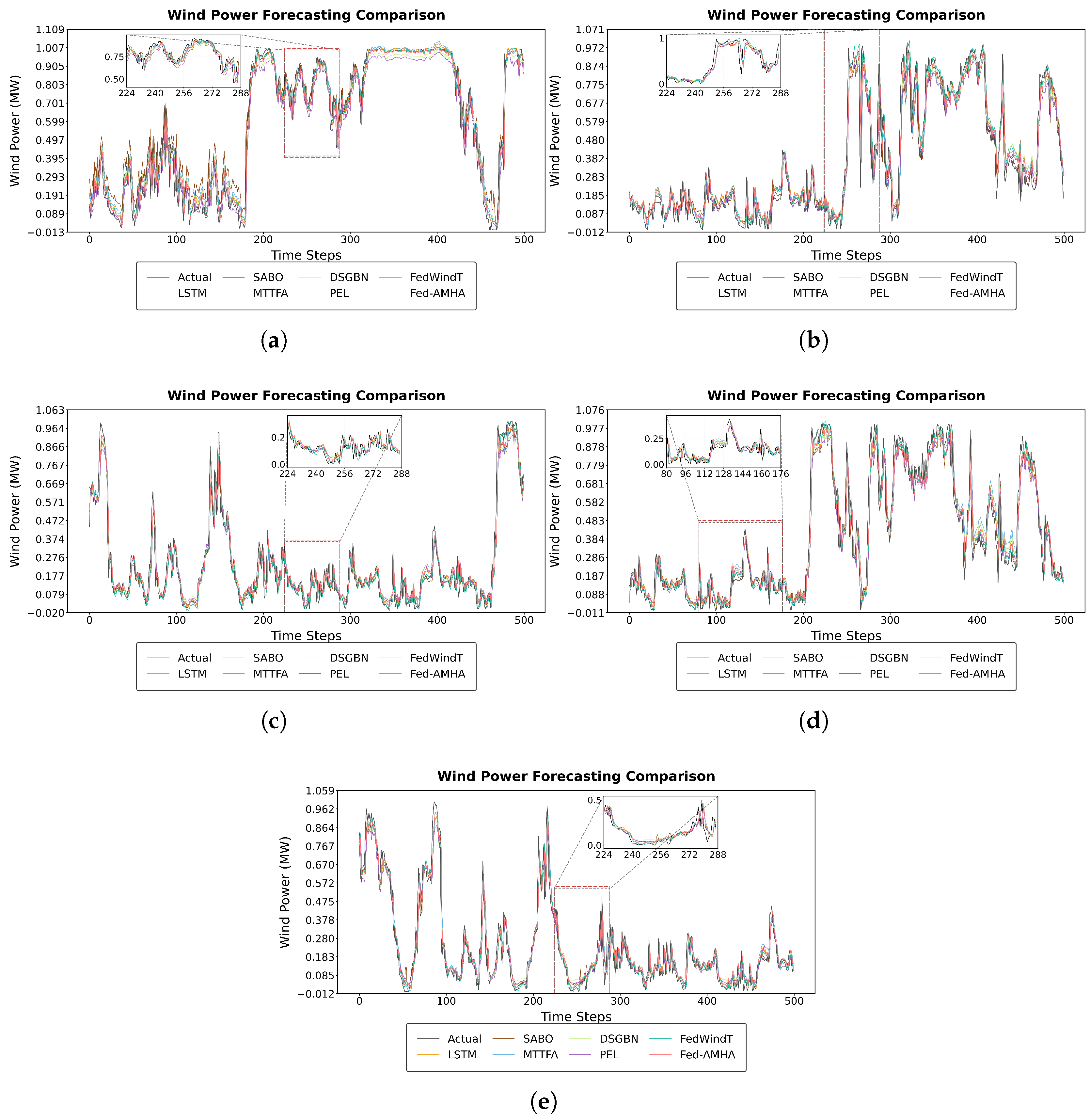
Figure 3 illustrates the prediction results of various models across different stations in the FuJian dataset. The visualization demonstrates that the proposed Fed-AMHA model consistently tracks the fluctuations of actual wind power across all stations. Specifically, the prediction curves exhibit high alignment with ground truth during stable periods, reflecting the model’s proficiency in capturing temporal dependencies. The robustness of Fed-AMHA is further evidenced during local volatile periods. For instance, at Station 1 (time steps 180–228), characterized by potential wind speed mutations or operational disturbances, Fed-AMHA maintains the minimum deviation compared to other models. In contrast, the DSGBN model exhibits significant lag and over-smoothing at power turning points, particularly at Stations 3 and 5, failing to recover high-frequency power details. In contrast, the prediction curves of the FedWindT and PEL models exhibit significant deviations from the ground truth. This is likely due to the absence of dedicated modules for handling data heterogeneity in both models. Specifically, as a lightweight Transformer, FedWindT is more sensitive to hyperparameters such as the learning rate, making it prone to underfitting or optimization instability. Meanwhile, PEL primarily relies on MLP-based fusion and possesses a weaker explicit temporal inductive bias, leading to degraded generalization performance when dealing with multi-station data characterized by significant operational variations. In summary, the cross-station results confirm that Fed-AMHA achieves superior overall accuracy and exceptional stability under local disturbances, benefiting from its effective modeling of coupled temporal and external factors.

5.5.5. Results Analysis Under Different Sampling Scales on the KDD CUP Dataset

The KDD CUP dataset comprises 134 wind turbines, from which data from five turbines were randomly sampled for visualization, as illustrated in Figure 4. The experimental results indicate that our proposed model achieves the superior performance in wind power forecasting for this dataset. As observed from the zoomed-in insets, during periods of significant power fluctuations, the power values predicted by our model consistently remain the closest to the ground truth, whereas the performance of other baseline models is largely comparable. Based on the experimental results in Section 5.5.4 and Section 5.5.5, we hypothesize that the primary reason Fed-AMHA achieves predictions closest to the ground truth lies in its Adaptive Multi-Head Attention mechanism. This mechanism utilizes learnable head weights to capture subtle power offsets across multiple subspaces. When coupled with the parallel 1D-CNN’s precise extraction of local patterns from heterogeneous variables, it significantly enhances the model’s transient response accuracy under multi-station heterogeneous data conditions.

5.5.6. Analysis of the Impact of Wind Speed Levels on Predictive Performance

To evaluate the predictive robustness of the model under varying wind environments, the original test set is partitioned into three subsets based on wind speed magnitude: TestDataset1 (low), TestDataset2 (medium), and TestDataset3 (high). For the KDD CUP dataset, the partition is based on the Wspd feature column; for the FuJian dataset, partitions are based on the 10 m and 100 m wind speed feature columns, respectively. The RMSE prediction errors for each subset are summarized in

Table 6. Prediction errors across different wind conditions (KDD CUP results shown in %).

Dataset	TestDataset1	TestDataset2	TestDataset3
KDD CUP Dataset	6.2409	9.8330	10.1373
FuJian 10 m Wind Speed	1.0072	2.0520	2.3682
FuJian 100 m Wind Speed	0.9788	1.6357	2.6765

.

As indicated by the results, both the KDD CUP and FuJian datasets exhibit a trend where prediction errors increase as wind speed intensifies. This observation aligns with the physical principles of wind power forecasting and can be primarily attributed to the nonlinear amplification of the power curve, the presence of high-velocity turbulence, and the increased operational complexity under high wind conditions.

5.5.7. Ablation Study

To verify the effectiveness of each module in the proposed Fed-AMHA, this section designs ablation control experiments. Five comparison strategies are established: w/o channel_attn (removing the channel attention module), w/o multi_head (removing the multi-head attention module), w/o 1D-CNN (removing the parallel 1D-CNN module), Central (centralized training), and Fed-AMHA (the full model). Experiments are conducted on the FuJian and KDD CUP datasets, with MSE, RMSE, NRMSE, MAE, and $R^2$ as evaluation metrics.

Table 7. Ablation study results on the Fujian dataset.

Metrics	w/o Channel_Attn	w/o Multi_Head	w/o 1D-CNN	w/o Spear	Central	Fed-AMHA
MSE	3.889	3.752	3.902	3.637	3.598	3.601
RMSE	1.972	1.937	1.975	1.907	1.897	1.897
MAE	1.313	1.235	1.328	1.177	1.139	1.147
$R^2$	0.947	0.949	0.946	0.950	0.951	0.951
NRMSE	0.0448	0.0440	0.0449	0.0433	0.0431	0.0431

and

Table 8. Ablation study results on the KDD CUP dataset.

Metrics	w/o Channel_Attn	w/o Multi_Head	w/o 1D-CNN	w/o Spear	Central	Fed-AMHA
MSE	0.781	0.780	0.782	0.787	0.772	0.747
RMSE	8.838	8.834	8.846	8.875	8.783	8.648
MAE	5.904	5.899	5.927	5.906	5.761	5.851
$R^2$	88.395	88.360	88.476	88.761	87.851	93.090
NRMSE	9.305	9.306	9.304	9.299	9.314	8.649

show the metric variation results of each model variant on the two datasets.

On the Fujian dataset, attention mechanisms enhance feature importance by adaptively weighting CNN channel outputs. Excluding them from Fed-AMHA (i.e., w/o attention) results in an 8.00% increase in MSE, a 14.47% increase in MAE, and a 0.42 drop in $R^2$, indicating that the loss of core features leads to degraded accuracy. Multi-head attention models temporal dependencies across multiple subspaces simultaneously. Removing it leaves only single-head attention, which fails to capture short-term fluctuations and long-term trends. This increases MSE by 4.19% and MAE by 7.67%. Furthermore, the parallel 1D-CNN module extracts local temporal details; removing it causes a significant 8.36% rise in MSE, a 15.77% rise in MAE, and a 0.53 drop in $R^2$, resulting in degraded predictive performance due to the loss of critical temporal information. Based on the Spearman correlation coefficient, feature selection filters out redundant noise and focuses on core physical attributes. Removing this module increases MSE by 1.02% and MAE by 2.64%. Given the homogeneous data distribution and low noise in Fujian, Fed-AMHA achieves performance comparable to centralized training, with no accuracy loss caused by federated aggregation.

The KDD CUP dataset exhibits severe distribution drift and local noise. Here, Spearman-based feature selection becomes critical: removing it leads to a 5.35% increase in MSE, a 2.62% increase in RMSE, and a 4.65% drop in $R^2$. Removing the parallel 1D-CNN, channel attention, and multi-head attention results in MSE increases of 4.75%, 4.56%, and 4.48%, respectively, along with significant $R^2$ degradation. Centralized training, which directly merges heterogeneous data, is vulnerable to distribution shifts, resulting in a 5.63% lower $R^2$ and a 7.68% higher NRMSE compared to Fed-AMHA. In summary, the ablation results on both datasets demonstrate that the collaboration of each module and the federated framework design effectively adapts to different data distributions, thereby improving prediction accuracy and model stability.

5.5.8. Communication Time Analysis

To evaluate the communication efficiency of the models, we recorded the average communication time per training round for each method. As shown in

Table 9. Average communication time per round for different models (s).

Dataset	SABO	MTTFA	LSTM	DSCBN	FedWindT	PEL	Fed-AMHA
FuJian	4.06	3.50	2.98	3.92	4.00	3.39	11.43
KDD CUP	11.75	11.04	8.95	11.27	13.98	10.63	30.62

, the communication overhead of the proposed Fed-AMHA is relatively high compared to the baselines. This can be primarily attributed to the increased computational complexity and parameter volume introduced by the large number of channels and attention heads within the adaptive channel attention and multi-head attention mechanisms.

Nevertheless, such a design significantly enhances the model’s ability to extract complex features. Experimental results demonstrate that our method achieves the highest prediction accuracy among all models. In precision-critical applications like wind power forecasting, the strategy of trading moderate computational overhead for substantial accuracy gains is of high practical value. Furthermore, the model maintains excellent real-time performance during the inference phase, with prediction latencies of only 0.2492 s and 0.1766 s for the KDD Cup and FuJian datasets, respectively.

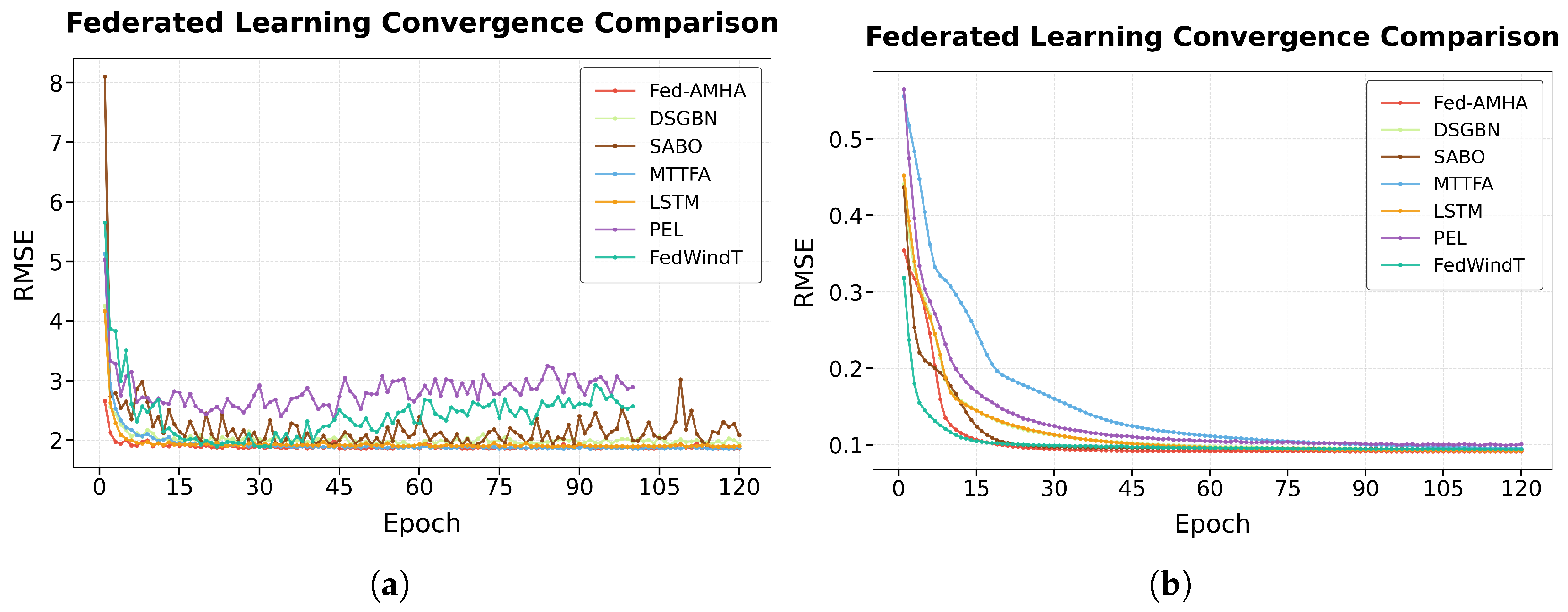
5.5.9. Model Convergence Analysis

From the perspective of the training convergence process, the proposed Fed-AMHA model exhibits superior optimization efficiency and stability on both datasets. As illustrated in Figure 5, on the FuJian dataset, the initial loss value of the Fed-AMHA model is lower than those of all baseline models, whereas the SABO model presents the highest initial loss. As training progresses, the loss of Fed-AMHA declines most rapidly and is the first to reach a stable converged state, reflecting robust gradient optimization capabilities and structural rationality. On the KDD CUP dataset, Fed-AMHA achieves suboptimal initial RMSE and convergence rates, while MTTFA converges slowest. Notably, unlike the stable convergence seen on KDD CUP, the PEL, FedWindT, and SABO models exhibit significant fluctuations on the FuJian dataset. This disparity suggests higher noise levels in the FuJian data, yet Fed-AMHA maintains efficient and stable convergence, demonstrating superior robustness to noise. The comprehensive analysis of the training process indicates that the Fed-AMHA model not only holds an advantage in prediction accuracy but also demonstrates faster convergence and better optimization stability during the training phase. This contributes to reducing training costs and enhancing engineering deployment efficiency. The disparities in the convergence curves further validate the effectiveness of the proposed structural design in terms of feature extraction and gradient propagation, providing a valuable reference for model optimization in wind power forecasting tasks.

6. Conclusions

To address the nonlinearity, data privacy, and multi-scale feature challenges in offshore wind power forecasting, this paper proposes a federated learning-based model integrated with adaptive multi-head attention (Fed-AMHA). The framework enables multi-party joint modeling while ensuring data privacy by keeping local data on-site. The model leverages Spearman correlation to reduce input redundancy and a BiLSTM network to capture historical power fluctuation patterns. Furthermore, a parallel 1D-CNN structure is integrated to extract spatial features across multiple scales. By employing channel attention and adaptive multi-head temporal attention, the model achieves precise weight allocation for critical features and time slices. Moreover, Fed-AMHA’s high scalability and decoupled architecture enable seamless transfer to other time-series tasks, including PV forecasting, wave energy assessment, and microgrid dispatching. Through task-specific attention adjustments, the framework effectively addresses feature heterogeneity across energy carriers, serving as a versatile foundation for cross-sector collaborative forecasting. Future work will focus on performance optimization under extreme weather (e.g., typhoons), model lightweighting for edge computing, and the integration of offshore fluid mechanics to develop a hybrid physics–data-driven model for enhanced robustness in small-sample scenarios.

References

1. Vargas, S.A.; Esteves, G.R.T.; Maçaira, P.M.; Bastos, B.Q.; Oliveira, F.L.C.; Souza, R.C. Wind power generation: A review and a research agenda. J. Clean. Prod. 2019, 218, 850–870. [Google Scholar] [CrossRef] [Scilit]
2. Mandzhieva, R.; Subhankulova, R. Data-driven applications for wind energy analysis and prediction: The case of “La Haute Borne” wind farm. Digit. Chem. Eng. 2022, 4, 100048. [Google Scholar] [CrossRef] [Scilit]
3. Haseeb, A.; Arshad, A.; Rehman, A.U.; Ashraf, M.M.; Hussain, G.A. Bayesian-Optimized Hybrid Deep Learning and Machine Learning Frameworks for Wind Power Forecasting. In 2025 IEEE PES Conference on Innovative Smart Grid Technologies-Middle East (ISGT Middle East); IEEE: Piscataway, NJ, USA, 2025; pp. 1–5. [Google Scholar]
4. Tsai, W.; Hong, C.; Tu, C.; Lin, W.; Chen, C. A Review of Modern Wind Power Generation Forecasting Technologies. Sustainability 2023, 15, 10757. [Google Scholar] [CrossRef] [Scilit]
5. Liu, S.; Zhu, Y.; Zhang, K.; Gao, J. Short term wind power forecasting based on error correction ARMA-GARCH model. Acta Energiae Solaris Sin. 2020, 41, 268–275. [Google Scholar]
6. Hammad, M.A.; Jereb, B.; Rosi, B.; Dragan, D. Methods and models for electric load forecasting: A comprehensive review. Logist. Supply Chain. Sustain. Glob. Chall. 2020, 11, 51–76. [Google Scholar] [CrossRef] [Scilit]
7. Khan, P.W.; Byun, Y.C.; Lee, S.J.; Kang, D.H.; Kang, J.Y.; Park, H.S. Machine learning-based approach to predict energy consumption of renewable and nonrenewable power sources. Energies 2020, 13, 4870. [Google Scholar] [CrossRef] [Scilit]
8. Lu, D.; Zhao, D.; Li, Z. Short-term nodal load forecasting based on machine learning techniques. Int. Trans. Electr. Energy Syst. 2021, 31, e13016. [Google Scholar] [CrossRef] [Scilit]
9. Messner, J.W.; Pinson, P. Online adaptive lasso estimation in vector autoregressive models for high dimensional wind power forecasting. Int. J. Forecast. 2019, 35, 1485–1498. [Google Scholar] [CrossRef] [Scilit]
10. Chen, N.; Qian, Z.; Nabney, I.T.; Meng, X. Short-Term Wind Power Forecasting Using Gaussian Processes. In Proceedings of the 23rd International Joint Conference on Artificial Intelligence, Beijing, China, 3–9 August 2013; IJCAI: Marina Del Rey, CA, USA, 2013; pp. 2790–2796. [Google Scholar]
11. Guan, S.; Wang, Y.; Liu, L.; Gao, J.; Xu, Z.; Kan, S. Ultra-short-term wind power prediction method based on FTI-VACA-XGB model. Expert Syst. Appl. 2024, 235, 121185. [Google Scholar] [CrossRef] [Scilit]
12. Zheng, X.; Luo, X.; Liu, D. A Novel Framework for Wind Power Prediction Based on Optimized Variational Mode Decomposition and Temporal Convolutional Network with Hybrid Attention. IEEE Power Electron. Mag. 2025, 12, 57–74. [Google Scholar] [CrossRef] [Scilit]
13. Hanifi, S.; Cammarono, A.; Zare-Behtash, H. Advanced hyperparameter optimization of deep learning models for wind power prediction. Renew. Energy 2024, 221, 119700. [Google Scholar] [CrossRef] [Scilit]
14. Liu, S.; Xu, T.; Du, X.; Zhang, Y.; Wu, J. A hybrid deep learning model based on parallel architecture TCN-LSTM with Savitzky-Golay filter for wind power prediction. Energy Convers. Manag. 2024, 302, 118122. [Google Scholar] [CrossRef] [Scilit]
15. Cheng, X.; Li, C.; Liu, X. A review of federated learning in energy systems. In 2022 IEEE/IAS Industrial and Commercial Power System Asia (I&CPS Asia), Shanghai, China, 8–11 July 2022; IEEE: Piscataway, NJ, USA, 2022; pp. 2089–2095. [Google Scholar]
16. Moradzadeh, A.; Moayyed, H.; Mohammadi-Ivatloo, B.; Vale, Z.; Ramos, C.; Ghorbani, R. A novel cyber-Resilient solar power forecasting model based on secure federated deep learning and data visualization. Renew. Energy 2023, 211, 697–705. [Google Scholar] [CrossRef] [Scilit]
17. Loukil, F.; El-Kouch, Y.; Verjus, H.; Vernier, F. A Federated Learning Framework for Wind Power Forecasting. In Proceedings of the IEEE International Conference on Distributed Computing Systems (ICDCS) Workshop on Federated Learning for Web Technologies (FL4WEB), Glasgow, UK, 21–23 July 2025. [Google Scholar]
18. Zhang, D.; Tian, W.; Cheng, X.; Shi, F.; Qiu, H.; Liu, X.; Chen, S. FedBIP: A federated learning-based model for wind turbine blade icing prediction. IEEE Trans. Instrum. Meas. 2023, 72, 3516011. [Google Scholar] [CrossRef] [Scilit]
19. Amer, H.N.; Dahlan, N.Y.; Azmi, A.M.; Latip, M.F.A.; Onn, M.S.; Tumian, A. Solar power prediction based on Artificial Neural Network guided by feature selection for Large-scale Solar Photovoltaic Plant. Energy Rep. 2023, 9, 262–266. [Google Scholar] [CrossRef] [Scilit]
20. Yang, X.; Wang, S.; Peng, Y.; Chen, J.; Meng, L. Short-term photovoltaic power prediction with similar-day integrated by BP-AdaBoost based on the Grey-Markov model. Electr. Power Syst. Res. 2023, 215, 108966. [Google Scholar] [CrossRef] [Scilit]
21. Sahin, G.; Isik, G.; van Sark, W.G. Predictive modeling of PV solar power plant efficiency considering weather conditions: A comparative analysis of artificial neural networks and multiple linear regression. Energy Rep. 2023, 10, 2837–2849. [Google Scholar] [CrossRef] [Scilit]
22. Ahmed, U.; Mahmood, A.; Tunio, M.A.; Hafeez, G.; Khan, A.R.; Razzaq, S. Investigating boosting techniques’ efficacy in feature selection: A comparative analysis. Energy Rep. 2024, 11, 3521–3532. [Google Scholar] [CrossRef] [Scilit]
23. Thipwangmek, N.; Woradit, K.; Suetrong, N.; Promsuk, N. Feature Selection Approaches for Short-Term Solar Photovoltaic Power Forecasting. In 2024 13th International Conference on Renewable Energy Research and Applications (ICRERA); IEEE: Piscataway, NJ, USA, 2024; pp. 252–257. [Google Scholar]
24. Ge, Y.; Zhang, W.; Liu, G.; Li, Z.; Li, H. Adaptive feature selection for probabilistic multi-energy load forecasting. IEEE Trans. Ind. Appl. 2023, 61, 1341–1351. [Google Scholar] [CrossRef] [Scilit]
25. Yang, Z.; Yang, B.; Zheng, R. Short-term Wind Power Prediction based on FFA-BiLSTM Algorithm. In 2025 IEEE 3rd International Conference on Power Science and Technology (ICPST); IEEE: Piscataway, NJ, USA, 2025; pp. 1455–1460. [Google Scholar]
26. Liu, X.; Zhou, J. Short-term wind power forecasting based on multivariate/multi-step LSTM with temporal feature attention mechanism. Appl. Soft Comput. 2024, 150, 111050. [Google Scholar] [CrossRef] [Scilit]
27. Yu, W.; Li, S.; Zhang, H.; Kang, Y.; Li, H.; Dong, H. Ultra-short-term wind-power forecasting based on an optimized CNN-BILSTM-attention model. iEnergy 2024, 3, 268–282. [Google Scholar] [CrossRef] [Scilit]
28. Rahmatinia, S.M.; Hosseini-Seno, S.A. An Attention-Based Deep Learning Model for Multi-Horizon Prediction of Load, Price, and Wind Power Generation in Smart Grids. In 2025 29th International Electrical Power Distribution Conference (EPDC), Tehran, Iran, 28–30 October 2025; IEEE: Piscataway, NJ, USA, 2025; pp. 1–9. [Google Scholar]
29. Shivkumar, S.; Singh, R.P.; Kumar, P. Wind power prediction using transformers: A federated learning approach. In 2023 9th International Conference on Signal Processing and Communication (ICSC); IEEE: Piscataway, NJ, USA, 2023; pp. 491–497. [Google Scholar]
30. Rahman, M.A.; Anwar, A.; Haque, M.E. Discriminative Scanner Enhanced Selective Partial Aggregation-based Federated Learning for Resilient and Efficient Wind Power Forecasting. IEEE Trans. Smart Grid 2025, 17, 1478–1491. [Google Scholar] [CrossRef] [Scilit]
31. Liu, J.; Zang, H.; Sun, K.; Sun, G.; Cheng, L.; Wei, Z. A Mode-Measurement-Cooperated Interaction Framework Based on Federated Split Learning for Regional Wind Power Forecasting. IEEE Trans. Smart Grid 2026. Early access. [Google Scholar] [CrossRef] [Scilit]
32. N, L.; Jayashri, R.; Ramya, M. Federated Learning-Based Res Forecasting in Smart Grids by Feature Fusion Using Cross Attention Mechanism. In 2025 2nd International Conference on Electronic Circuits and Signaling Technologies (ICECST), Petaling Jaya, Malaysia, 23–25 October 2025; IEEE: Piscataway, NJ, USA, 2025; pp. 420–425. [Google Scholar]
33. Zhou, J.; Lu, X.; Xiao, Y.; Su, J.; Lyu, J.; Ma, Y.; Dou, D. Sdwpf: A dataset for spatial dynamic wind power forecasting challenge at kdd cup 2022. arXiv 2022, arXiv:2208.04360. [Google Scholar] [CrossRef] [Scilit]
34. He, X.; Ma, Y.; Xie, J.; Zhang, G.; Xie, T. Enhanced Wind Power Forecasting Using Graph Convolutional Networks with Ramp Characterization and Error Correction. Energies 2025, 18, 2763. [Google Scholar] [CrossRef] [Scilit]
35. Arooj, Q. FedWindT: Federated learning assisted transformer architecture for collaborative and secure wind power forecasting in diverse conditions. Energy 2024, 309, 133072. [Google Scholar] [CrossRef] [Scilit]
36. Rong, J.; Liu, W.; Jiang, F.; Yang, Y. Geographical distributed turbine power prediction using personalized federated learning. Expert Syst. Appl. 2026, 303, 130584. [Google Scholar] [CrossRef] [Scilit]
Figure 1. Framework of the wind power prediction model.
Bdcc 10 00147 g001
Figure 2. Visualization of performance results for different models across various datasets: (a) Results on the FuJian dataset; (b) Results on the KDD CUP dataset.
Bdcc 10 00147 g002
Figure 3. Predictive performance of various models across different sites on the FuJian dataset: (a) Performance at Site 1. (b) Performance at Site 2. (c) Performance at Site 3. (d) Performance at Site 4. (e) Performance at Site 5.
Bdcc 10 00147 g003
Figure 4. Predictive performance of various models across different sites on the KDD CUP dataset: (a) Performance at Turbine 1. (b) Performance at Turbine 2. (c) Performance at Turbine 3. (d) Performance at Turbine 4. (e) Performance at Turbine 5.
Bdcc 10 00147 g004
Figure 5. Convergence performance across different datasets: (a) On the FuJian dataset; (b) on the KDD CUP dataset.
Bdcc 10 00147 g005