A Reservoir Computing Approach for Synchronizing Discrete-Time 3D Chaotic Systems

Abstract

Reservoir computing (RC) is an efficient framework for processing time-series data. This work investigates the synchronization of two independently trained reservoir computers that, after training, operate without external input from the chaotic system and interact solely through symmetric linear coupling. This approach addresses a gap in existing reservoir computing-based synchronization studies, which predominantly rely on master–slave or system-driven configurations. In this work, we first build and train two reservoir computing models based on 3D nonlinear chaotic maps and hyperchaotic systems and then introduce a symmetric linear coupling mechanism between them. This study demonstrates that reservoir computing can accurately reproduce the short-term dynamics of chaotic systems and provides insight into the interactions between learned dynamical models, while also helping us understand how complex systems connect and operate collectively. We use this systematic approach to establish a framework for understanding how two trained reservoir computers interact under varying coupling strengths, enabling a detailed investigation of their synchronization behavior. To demonstrate the adaptability of the proposed framework to diverse dynamical behaviors, we systematically investigated three discrete chaotic and hyperchaotic systems: (1) discrete 3D sinusoidal map with discrete Lorenz attractor, (2) 3D sinusoidal map with conjoined Lorenz twin attractor, and (3) 3D quadratic hyperchaotic map. For performance evaluation, we trained coupled RCs and computed the synchronization error for different coupling strengths. We also present phase portraits and time-series plots of the attractors and RCs, along with the synchronization error as a function of the coupling strength, thereby demonstrating the possibility of synchronization of two linearly coupled RCs, which are independently trained on discrete, three-dimensional chaotic and hyperchaotic systems.

1. Introduction

Reservoir computing (RC) has emerged as an efficient and robust framework for modeling complex temporal dynamics [1], particularly in nonlinear and chaotic systems [2,3]. By using a fixed high-dimensional dynamical system (the reservoir) and training only a linear readout layer, RC provides a computationally efficient alternative to traditional recurrent neural networks [4]. This simplicity, combined with its ability to capture nonlinear temporal dependencies, makes RC well-suited for real-time prediction and analysis of chaotic dynamical systems [5,6,7]. In recent years, RC has demonstrated strong performance in forecasting chaotic time series [8], reconstructing attractors [9], and modeling complex dynamical behavior [10] without requiring explicit knowledge of governing equations [11,12,13]. Owing to the Echo State Property (ESP), reservoirs driven by external inputs can synchronize with the underlying system dynamics, enabling accurate short-term prediction and state reconstruction. This has led to widespread applications in physics [14], engineering [15], and data-driven modeling of nonlinear systems [16].

A growing body of research has explored synchronization in reservoir computing frameworks. Early studies primarily focused on externally driven synchronization [17], where the reservoir is continuously supplied with input signals from the original system. Subsequent works extended this idea to master–slave configurations, where a slave reservoir synchronizes with a driving system through unidirectional coupling [18,19]. More recent studies have considered coupling between multiple reservoirs [20]. However, such approaches rely on external inputs or hierarchical driving mechanisms [21]. A key limitation shared by these approaches is their dependence on external signals or predefined hierarchical structures to enforce synchronization. In many practical scenarios, multiple intelligent units trained on similar data must function without continuous external input or centralized coordination. Distributed sensing, decentralized control, secure communication [22], etc., require synchronization without continuous access to external signals. In such cases, synchronization must arise from mutual interaction within the system rather than external forcing. Therefore, understanding whether learned dynamical models can synchronize with each other through simple interaction rules remains an important open question [23]. In particular, it is unclear whether two independently trained reservoirs, each capable of reproducing the dynamics of a chaotic system, can achieve synchronization with each other solely through mutual interaction.

From a dynamical systems perspective, this problem is closely related to the broader question of whether learned models can exhibit collective behavior similar to coupled physical systems [24]. In classical synchronization theory, interaction between systems is often modeled through diffusive or linear coupling, which enables information exchange [25] while preserving individual system dynamics. Extending this concept to reservoir computing raises important questions about the interplay between learned representations and coupling mechanisms. In particular, it becomes essential to investigate whether synchronization observed in such systems reflects genuine alignment of internal dynamics rather than an artifact of training or numerical approximation.

In this work, we propose a framework for synchronizing two independently trained and fully autonomous reservoir computers using symmetric linear coupling [23]. After training on chaotic time-series data, both reservoirs operate in a closed-loop configuration without further external input. The interaction between the systems is introduced solely through a convex combination of their outputs, enabling mutual coupling without a master–slave hierarchy. This setup allows us to investigate whether synchronization can emerge purely from interaction between learned dynamical systems. Unlike existing reservoir computing approaches that rely on external driving signals or unidirectional coupling, the proposed framework enables synchronization in a fully autonomous setting. This represents a shift from externally enforced synchronization to interaction-induced synchronization, where collective behavior arises intrinsically from the dynamics of coupled learned models. To further clarify this distinction, a comparative summary with existing approaches is provided in

Table 1. Comparison of the proposed RC method with existing approaches.

Method	External Input	Autonomous	Mutual Coupling	Primary Objective
RC with external driving [26]	Yes	No	No	Prediction
Master–slave RC synchronization [27]	Yes	No	No	Synchronization
Coupled RC with input driving [20]	Yes	No	Partial	Synchronization
Proposed method	No	Yes	Yes	Autonomous synchronization

. Reservoir computing has been extensively studied for modeling, prediction, and synchronization of chaotic dynamical systems. Early works established the ability of echo state networks to learn complex temporal dynamics and reconstruct attractors from observed time series. Subsequent studies demonstrated that reservoir computers can achieve synchronization with chaotic systems under external driving conditions, often within master–slave or driver–response configurations. More recent research has explored interactions between multiple reservoirs; however, these approaches typically rely on continuous external inputs or asymmetric coupling structures. In contrast to these existing approaches, the present work focuses on synchronization between two independently trained reservoir computers operating in a fully autonomous regime, where interaction occurs solely through symmetric linear coupling. This setting removes dependence on external driving signals and enables the study of intrinsic collective dynamics between learned systems, which has received comparatively limited attention in the prior literature.

The main contributions of this work are summarized as follows:

• We propose a framework for synchronizing two independently trained and autonomous reservoir computers using symmetric linear coupling.
• We investigate whether symmetric linear coupling can achieve synchronization between two autonomous reservoir computers, quantified using the average synchronization error,

  $$\Delta ={\displaystyle \frac{1}{T_{\mathrm{sync}}}}\sum _{t=1}^{T_{\mathrm{sync}}}∥y_1\left(t\right)-y_2\left(t\right)∥,$$

  (1)

  where $y_1\left(t\right)$ and $y_2\left(t\right)$ denote the output vectors of the two reservoir computers at time step t, and $T_{\mathrm{sync}}$ represents the total number of time steps over which the coupled systems evolve during the synchronization phase. The synchronization error is computed as the average difference between the outputs over this duration.
• We systematically evaluate synchronization behavior across multiple discrete-time, three-dimensional chaotic and hyperchaotic systems, revealing system-dependent coupling regimes.
• In the results section, we present the plots of synchronization error vs. coupling strength between the reservoir computers. We also provide the phase portraits and time series of the attractor and RCs.

The paper is organized as follows: In Section 2, we present a flowchart illustrating the key steps involved in the overall process of synchronizing the reservoir computers. In Section 3, we describe the coupling scheme, training procedure, and simulation setup. In Section 4, we present the experimental results, including synchronization behavior under varying coupling strengths. The paper concludes with a summary of the findings and directions for future research.

2. Workflow

In reservoir computing, a distinction is typically made between a training phase, during which the system is driven by external input signals, and a closed-loop phase, in which the trained model evolves without external driving. In this work, we consider two post-training regimes. First, we examine the fully autonomous regime, where each reservoir operates independently in a closed loop, driven solely by its own output feedback and without any coupling or external input. Second, we consider a coupled autonomous regime in which the reservoirs remain free of external driving but are mutually coupled via a symmetric linear mechanism. In both cases, the dynamics are entirely self-sustained, with no external inputs applied after training. This distinction allows us to separately analyze the intrinsic dynamics learned by each reservoir and the emergence of synchronization solely due to inter-reservoir coupling.

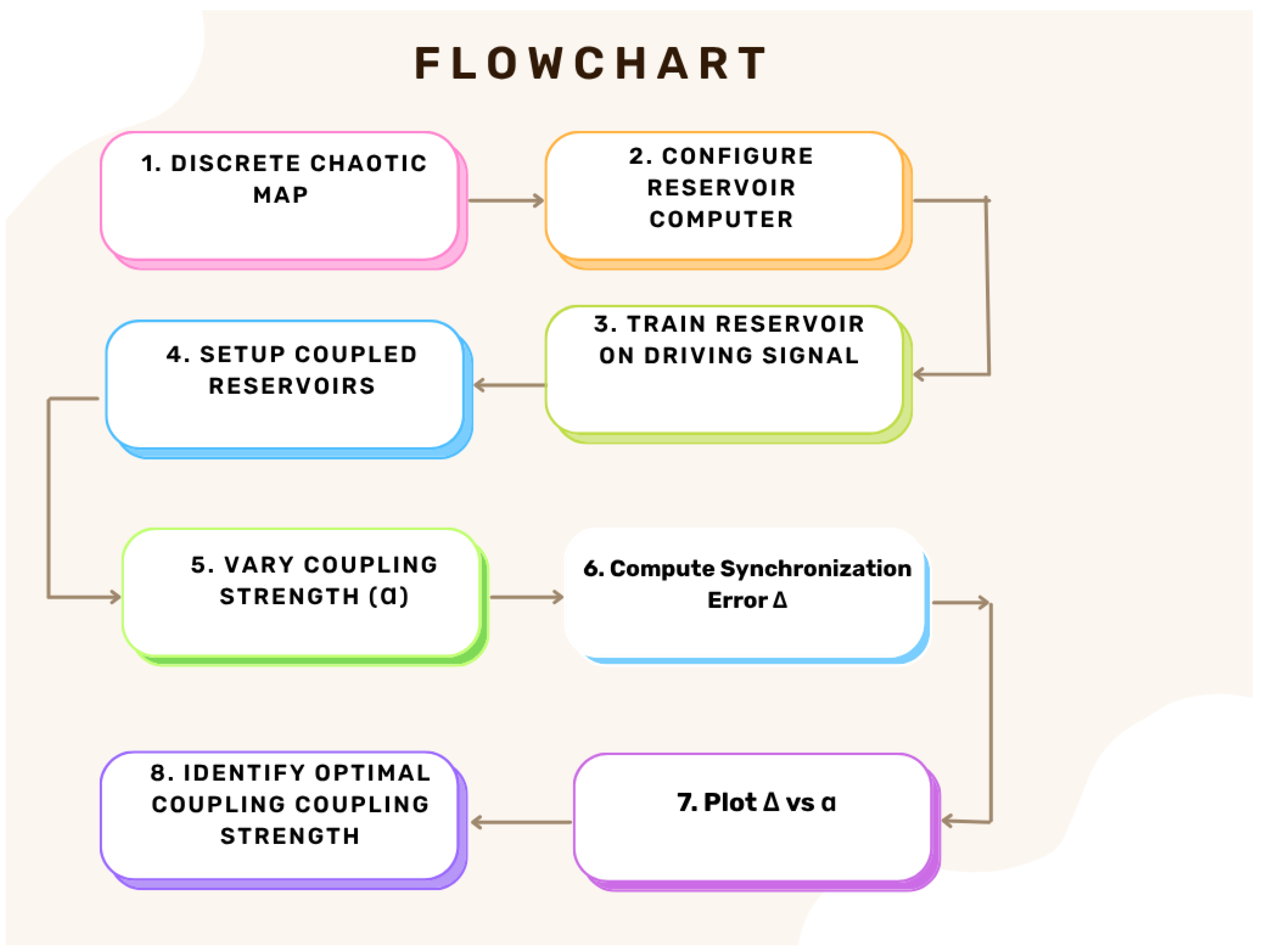
Figure 1 provides an overview of the complete synchronization workflow and serves as a visual guide for the methodology described in the following section. The flowchart summarizes the sequential procedure adopted to achieve synchronization between reservoir computers driven by discrete-time chaotic systems. The process begins with the definition of the underlying discrete-time chaotic or hyperchaotic systems. In this work, the dynamics are generated using a discrete 3D sinusoidal map, a 3D sinusoidal map with conjoined Lorenz twin attractor, and a 3D quadratic hyperchaotic map. From these maps, time-series data are obtained by discarding initial transients, ensuring that the trajectories lie on the attractor. The resulting time series is then used to train the reservoir computers.

Next, two reservoir computers are independently initialized. Each reservoir is constructed as a sparse Erdős–Rényi random network with a specified number of nodes (N) and average degree (d). The non-zero entries of the reservoir weight matrix are randomly assigned and subsequently rescaled to achieve a desired spectral radius ($\rho$). The input weight matrices are initialized randomly from a uniform distribution, and the reservoir states are initialized to zero at the beginning of training. The two reservoir computers are then trained independently using the same time-series data. During training, the reservoir states are driven by the input signal, and the output weights are computed using ridge regression [28]. This training procedure enables each reservoir to learn the underlying dynamics of the chaotic system and reproduce its behavior in an autonomous mode.

Following training, the reservoirs are operated in a closed-loop configuration, where their outputs are fed back as inputs. A symmetric, linear coupling is introduced between the two reservoirs. The coupling strength is controlled by the parameter $\alpha$. Specifically, the input to each reservoir is constructed as a convex combination of its own output and the other reservoir’s output, thereby enabling interaction between the two autonomous systems. To quantify synchronization, the coupled reservoirs are evolved over a fixed number of time steps, and the synchronization error $\Delta$ is computed as the average Euclidean distance between their output trajectories. This procedure is repeated for a range of coupling strengths $\alpha \in [0,1]$, allowing the construction of synchronization error curves as a function of coupling strength $\alpha$.

The primary objective of this analysis is to identify the range of coupling strengths that minimizes the synchronization error, thereby indicating the emergence of synchronized dynamics between the two reservoir computers. The system architecture and synchronization methodology are described in detail in Section 3.

3. System Architecture and Synchronization Method

3.1. Reservoir Computer Configuration

In this work, we first construct and train two reservoir computing models using time-series data generated by chaotic systems. After training, the two models are paired through a symmetric linear coupling scheme in order to investigate their interaction and synchronization behavior over time. Reservoir computing is a machine learning framework derived from recurrent neural networks (RNNs) [29], and is particularly well suited for modeling and analyzing temporal data. In the present study, the reservoir computers are trained using discrete-time chaotic input signals.

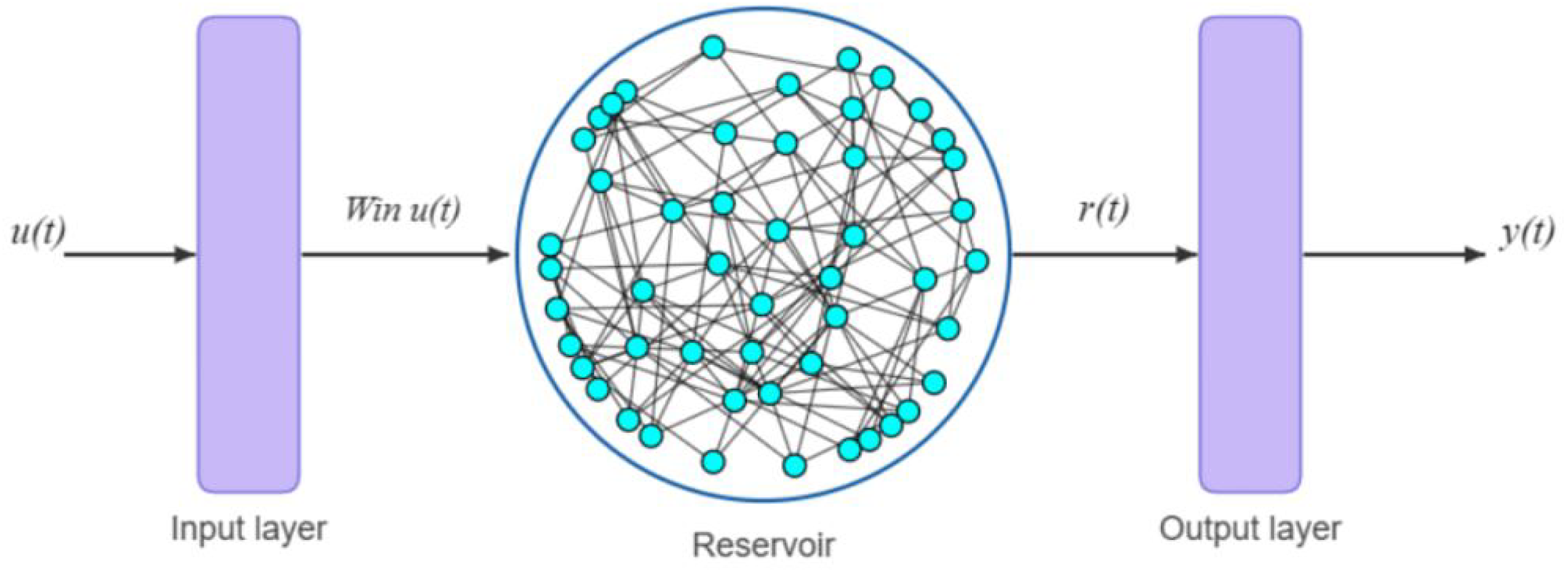
The reservoir computing architecture employed in this work consists of three main components: an input layer, a reservoir layer, and an output (readout) layer (see Figure 2). The input layer injects the chaotic time-series signals into the reservoir. The reservoir layer, composed of a large number of sparsely interconnected nonlinear nodes, serves as the dynamical core of the system and transforms the input into a high-dimensional state representation. The reservoir connectivity is generated using the Erdős–Rényi (ER) random graph model [30], one of the most widely used and well-studied models for constructing random networks. Finally, the output layer is a trainable linear readout that maps the reservoir states and the input signals to the desired system output.

The reservoir networks are generated using the Erdős–Rényi random graph model with a fixed random seed to ensure reproducibility. The reservoir dynamics are governed by the standard discrete-time echo state network update rule. We do not employ leaky integration, as the discrete-time formulation is sufficient for modeling the map-based chaotic systems considered here. The state update equation is given by

$$\mathbf{r}(t+1)=tanh\left[A\mathbf{r}\left(t\right)+W_{\mathrm{in}}\mathbf{u}\left(t\right)\right],$$

(2)

where $\mathbf{r}\left(t\right)\in {\mathbb{R}}^N$ is the reservoir state vector, $\mathbf{u}\left(t\right)\in {\mathbb{R}}^D$ is the input vector, $A\in {\mathbb{R}}^{N\times N}$ is the reservoir (recurrent) weight matrix, and $W_{\mathrm{in}}\in {\mathbb{R}}^{N\times D}$ is the input weight matrix. The reservoir output is computed using a linear readout of the reservoir state and input as

$$\mathbf{y}\left(t\right)=W_{\mathrm{out}}\left[\begin{array}{c}\mathbf{u}\left(t\right)\\ \mathbf{r}\left(t\right)\end{array}\right],$$

(3)

where $\mathbf{y}\left(t\right)\in {\mathbb{R}}^D$ is the output vector and $W_{\mathrm{out}}\in {\mathbb{R}}^{D\times (D+N)}$ is the output weight matrix.

The main parameters of the reservoir computer are the network size N, which refers to the total number of nodes (neurons) in the reservoir, average degree d, which represents the average number of connections each node has within the reservoir, and spectral radius $\rho$, which is the largest absolute eigenvalue of the reservoir’s weight matrix A. A tanh activation function is employed to ensure bounded and stable reservoir states. The reservoir weight matrices A are initialized with non-zero entries drawn from a uniform distribution and subsequently rescaled to achieve the desired spectral radius $\rho$. The input weight matrices $W_{in}$ are initialized from a uniform distribution. Initial reservoir states are randomly generated from a small-amplitude uniform distribution. A more detailed description is given in

Table 2. Reservoir computer architecture and training parameters used across all experiments.

Parameter	Value/Description
Reservoir topology	Erdős–Rényi random graph
Reservoir size (N)	800–1000 (system-dependent; see Table 3)
Average degree (d)	10–20
Spectral radius ($\rho$)	0.9–1.8
Input/output dimension (D)	3
Activation function	$tanh(·)$
Input weight initialization ($W_{in}$)	Uniform random distribution
Reservoir weight initialization (A)	Uniform random, rescaled to $\rho$
Initial reservoir state ($\mathbf{r}\left(0\right)$)	Small random values
Regularization parameter ($\lambda$)	${10}^{-6}$
Training duration (T)	10,000 iterations
Synchronization duration with coupled reservoirs ($T_{\mathrm{sync}}$)	10,000 iterations
Coupling type	Symmetric linear coupling
Coupling strength ($\alpha$)	100 uniformly spaced points over the interval $[0,1]$
Synchronization error ($\Delta \left(t\right)$)	$\Delta \left(t\right)=\langle \parallel {\mathbf{y}}_1\left(t\right)-{\mathbf{y}}_2\left(t\right)\parallel \rangle$
Number of trials ($N_{\mathrm{trials}})$	10

. The chaotic system time-series data are generated at fixed, discrete time steps. Before being used as reservoir inputs, each time series is normalized to have zero mean and unit variance. The specific reservoir parameters used for each of the three discrete-time chaotic systems are summarized in

Table 3. Reservoir computer parameters for the simulation of chaotic systems.

System	N	d	$\mathit{\rho }$
Discrete 3D sinusoidal map with discrete Lorenz attractor	800	20	1.8
3D sinusoidal map with conjoined Lorenz twin attractor	1000	20	1.8
3D quadratic hyperchaotic map	1000	20	1.8

.

3.2. Training Procedure and Autonomous Operation

The training process involves feeding time-series data from one of three discrete, chaotic systems (a discrete 3D sinusoidal map, a 3D sinusoidal map with a conjoined Lorenz twin attractor, and a 3D quadratic hyperchaotic map) into the reservoir network. This setup enables accurate time-series predictions and facilitates short-term simulation of the system’s attractor, as in [23]. During training, the reservoir computer is provided with an input time series $\mathbf{u}\left(t\right)$ generated from the chaotic system, and the state of the reservoir $\mathbf{r}\left(t\right)$ is updated according to Equation (2) and recorded along with the respective input at each time step. Considering N as the size of the reservoir, D as the dimension of the time series given as input to the system, and T as the number of time steps used for training the system. To eliminate the effect of initial conditions, an initial washout period is applied during training, during which reservoir states are updated but not recorded. This ensures that the collected states used for training reflect the reservoir’s intrinsic dynamics rather than initialization artifacts.

The extended reservoir state at time t is defined as

$$\mathbf{x}\left(t\right)=\left[\begin{array}{c}\mathbf{u}\left(t\right)\\ \mathbf{r}\left(t\right)\end{array}\right]\in {\mathbb{R}}^{D+N},$$

(4)

where $\mathbf{u}\left(t\right)\in {\mathbb{R}}^D$ denotes the input vector and $\mathbf{r}\left(t\right)\in {\mathbb{R}}^N$ the reservoir state.

Collecting these extended states over time yields the state matrix

$$\mathbf{X}\in {\mathbb{R}}^{(D+N)\times T},$$

(5)

and the corresponding target matrix

$$\mathbf{Y}\in {\mathbb{R}}^{D\times T}.$$

(6)

where $\mathbf{Y}$ contains the target outputs.

The ridge regression solution for the output weight matrix is given by

$$W_{\mathrm{out}}=\mathbf{Y}{\mathbf{X}}^{\top }{\left(\mathbf{X}{\mathbf{X}}^{\top }+\lambda \mathbf{I}\right)}^{-1},$$

(7)

where $W_{\mathrm{out}}\in {\mathbb{R}}^{D\times (D+N)}$ and $\lambda$ is the non-negative regularization parameter. The regularization prevents overfitting by penalizing large weights.

The matrix being inverted $\mathbf{X}{\mathbf{X}}^{\top }+\lambda \mathbf{I}$ has dimension $(D+N)\times (D+N)$ and is independent of the number of training samples T.

As discussed above, the reservoir computers are trained using input signals obtained by extracting the state variables of the respective chaotic systems at a fixed sampling rate over a total of 10,000 iterations. These extracted signals serve as training data, enabling the reservoirs to learn the underlying system dynamics. To generate the input signals, we employ the discrete-time chaotic systems described earlier. The specific reservoir parameters used for each of the three discrete-time chaotic systems are summarized in Table 3.

The reservoir hyperparameters (including reservoir size N, spectral radius $\rho$ and average degree d) were selected empirically for each system based on preliminary experiments to ensure stable reservoir dynamics and accurate reconstruction of the underlying attractor. In particular, parameter values were chosen so that the reservoir operates in a dynamical regime that reliably captures the characteristics of the driving chaotic system prior to coupling. Variation in parameter settings across systems reflects differences in their intrinsic dynamical properties. A systematic investigation of parameter sensitivity and optimization, including the impact of these parameters on synchronization performance, is beyond the scope of the present work and will be considered in future studies.

After training, the external input from the original system is completely removed, and both reservoir computers operate in an autonomous mode. In this post-training phase, each reservoir is evolved independently in a closed-loop (fully autonomous) configuration for a duration of $T_{\mathrm{sync}}$ time steps. This autonomous run provides a consistent baseline state prior to the introduction of coupling.

3.3. Coupling Mechanism Design

After completion of the training phase, both reservoir computers operate as autonomous dynamical systems. We then introduce a linear coupling mechanism to enable interaction between them. Linear coupling is chosen because it represents one of the simplest and most fundamental forms of interaction in dynamical systems. It naturally arises in practical scenarios where signals are combined through weighted averaging or superposition, such as in communication systems, distributed sensor networks, and networked control systems. Moreover, linear (diffusive) coupling has been extensively studied in the context of coupled oscillators and nonlinear dynamics, where it serves as a basic mechanism for information exchange leading to synchronization. Its simplicity and analytical tractability make it particularly suitable for investigating collective behavior. In the present work, the use of linear coupling allows us to systematically study whether synchronization can emerge purely from the interaction between independently trained reservoir computers, without introducing additional nonlinear complexities. A similar coupling approach for continuous systems has been reported in the literature [23]. This makes it a suitable choice to investigate the synchronization properties between learned reservoirs while maintaining the dynamics within the reservoirs. The coupling mechanism between the two reservoir computers is linear and symmetric, and is given by

$${\mathbf{u}}_1(t+1)=\alpha {\mathbf{y}}_2\left(t\right)+(1-\alpha ){\mathbf{y}}_1\left(t\right),$$

(8)

$${\mathbf{u}}_2(t+1)=\alpha {\mathbf{y}}_1\left(t\right)+(1-\alpha ){\mathbf{y}}_2\left(t\right),$$

(9)

where ${\mathbf{u}}_1\left(t\right)$ and ${\mathbf{u}}_2\left(t\right)$ denote the input signals to reservoir computers 1 and 2, respectively, and ${\mathbf{y}}_1\left(t\right)$ and ${\mathbf{y}}_2\left(t\right)$ are their corresponding outputs. The parameter $\alpha \in [0,1]$ represents the coupling strength. If the $\alpha$ value is very small (i.e., close to zero), then the interaction between the reservoir computers is minimal, and thus, negligible synchronization happens. When the $\alpha$ reaches an intermediate value, the mutual interaction becomes strong, and this leads to synchronization. When the coupling strength $\alpha$ approaches 1, the coupling becomes effectively unidirectional in the sense that each reservoir is predominantly driven by the output of the other system. Thus, the input at the next time step $\mathbf{u}(t+1)$ is a weighted combination of the present outputs of both reservoir computers. In this paper, the coupling strength $\alpha$ is varied in 100 uniformly spaced steps over the interval [0, 1], and the synchronization between the two reservoir computers is analyzed.

When trained on highly unpredictable chaotic signals, the reservoir computer can effectively approximate the underlying system dynamics up to a finite accuracy. The phase portraits generated by reservoir computers closely match those of the original systems. This has also been validated using power spectra and Poincaré return maps in the literature [23]. As mentioned before, after the training, the reservoir computer operates autonomously. Now we then investigate their collective behavior under mutual interaction between two reservoir computers, and we also analyze whether they can achieve synchronization when they are coupled together. In this context, synchronization refers to the alignment of the dynamical states of the two reservoir computers over time, i.e., ${\mathbf{y}}_1\left(t\right)\approx {\mathbf{y}}_2\left(t\right)$, where ${\mathbf{y}}_1\left(t\right)$ and ${\mathbf{y}}_2\left(t\right)$ denote their respective output vectors at time t.

3.4. Synchronization Error Calculation

To quantitatively evaluate the degree of synchronization between the two reservoir computers, we employ a synchronization error metric defined in Equation (1). This metric quantifies how closely the outputs of the two systems align over time. Thus, through this systematic approach, we establish a framework of how two trained reservoir computers interact under varying coupling strengths, enabling a detailed investigation of their synchronization behavior. To address the sensitivity of reservoir computing performance to random initialization of the reservoir and input weights, all synchronization experiments were repeated over multiple independent trials. Specifically, for each coupling strength $\alpha$, we conducted 10 independent trials with different random input weight initializations while keeping the reservoir topology fixed by following the procedure outlined in Algorithm 1 and the description given in Table 4. The synchronization error was then averaged across trials, and the corresponding standard deviation was computed. All reported synchronization curves therefore represent the mean synchronization error. This procedure ensures the statistical robustness of the results by confirming that the observed synchronization behavior is not attributable to a particular random initialization.

Table 4. Definition of symbols and variables employed in the proposed reservoir computing framework and Algorithm 1. It includes parameters related to network structure, training, coupling, and synchronization evaluation.

Symbol	Description
N	Number of reservoir nodes
d	Average degree of the Erdős–Rényi reservoir graph
$p={\displaystyle \frac{d}{N}}$	Connection probability of the Erdős–Rényi graph
$\rho$	Spectral radius of the reservoir weight matrix
$\lambda$	Ridge regularization parameter
$\alpha$	Coupling strength parameter
${\alpha }_{min}$	Coupling strength minimizing average synchronization error
T	Length of training time series
$T_{\mathrm{sync}}$	Synchronization simulation length
$N_{\mathrm{trials}}$	Number of independent trials
$\mathbf{u}\left(t\right)$	Input time-series vector at time t
${\mathbf{u}}_1\left(t\right),{\mathbf{u}}_2\left(t\right)$	Coupled inputs to RC1 and RC2
${\mathbf{r}}_1\left(t\right),{\mathbf{r}}_2\left(t\right)$	Reservoir state vectors of RC1 and RC2
${\mathbf{y}}_1\left(t\right),{\mathbf{y}}_2\left(t\right)$	Output state vectors of RC1 and RC2
$A_1,A_2$	Reservoir recurrent weight matrices
$W_{\mathrm{in},1},W_{\mathrm{in},2}$	Input weight matrices
$W_{\mathrm{out},1},W_{\mathrm{out},2}$	Output weight matrices
$X_i,Y_i$	State and target matrices used for training
$\Delta \left(t\right)$	Instantaneous synchronization error at time t
${\Delta }^{\left(n\right)}\left(\alpha \right)$	Trial synchronization error for trial n and coupling $\alpha$
$\Delta \left(\alpha \right)$	Average synchronization error over trials

Table 4. Definition of symbols and variables employed in the proposed reservoir computing framework and Algorithm 1. It includes parameters related to network structure, training, coupling, and synchronization evaluation.

Symbol	Description
N	Number of reservoir nodes
d	Average degree of the Erdős–Rényi reservoir graph
$p={\displaystyle \frac{d}{N}}$	Connection probability of the Erdős–Rényi graph
$\rho$	Spectral radius of the reservoir weight matrix
$\lambda$	Ridge regularization parameter
$\alpha$	Coupling strength parameter
${\alpha }_{min}$	Coupling strength minimizing average synchronization error
T	Length of training time series
$T_{\mathrm{sync}}$	Synchronization simulation length
$N_{\mathrm{trials}}$	Number of independent trials
$\mathbf{u}\left(t\right)$	Input time-series vector at time t
${\mathbf{u}}_1\left(t\right),{\mathbf{u}}_2\left(t\right)$	Coupled inputs to RC1 and RC2
${\mathbf{r}}_1\left(t\right),{\mathbf{r}}_2\left(t\right)$	Reservoir state vectors of RC1 and RC2
${\mathbf{y}}_1\left(t\right),{\mathbf{y}}_2\left(t\right)$	Output state vectors of RC1 and RC2
$A_1,A_2$	Reservoir recurrent weight matrices
$W_{\mathrm{in},1},W_{\mathrm{in},2}$	Input weight matrices
$W_{\mathrm{out},1},W_{\mathrm{out},2}$	Output weight matrices
$X_i,Y_i$	State and target matrices used for training
$\Delta \left(t\right)$	Instantaneous synchronization error at time t
${\Delta }^{\left(n\right)}\left(\alpha \right)$	Trial synchronization error for trial n and coupling $\alpha$
$\Delta \left(\alpha \right)$	Average synchronization error over trials

Algorithm 1 Training and Synchronization of Coupled Reservoir Computers for Discrete-time Chaotic Systems

Input: Training series ${\left\{\mathbf{u}\left(t\right)\right\}}_{t=1}^T$, reservoir parameters $(N,d,\rho ,\lambda )$, coupling set ${\left\{\alpha \right\}}_{j=1}^M$, synchronization length $T_{\mathrm{sync}}$, number of trials $N_{\mathrm{trials}}=10$

Output: Optimal coupling strength ${\alpha }_{min}$

1: Initialize storage for $\Delta \left(\alpha \right)$ for all j

2: for $n=1$ to $N_{\mathrm{trials}}$ do

Training Phase

3:     Generate two independent Erdős Rényi random graphs $G_1, G_2$ with N nodes and connection probability $p={\displaystyle \frac{d}{N}}$

4:     Construct reservoir matrices $A_1,A_2$ from $G_1,G_2$ with random weights and scale them to the spectral radius $\rho$

5:     Initialize random input weight matrices $W_{\mathrm{in},1},W_{\mathrm{in},2}$

6:     Initialize ${\mathbf{r}}_1\left(0\right);{\mathbf{r}}_2\left(0\right)$

7:     for $t=1$ to T do

8:           ${\mathbf{r}}_i\left(t\right)=tanh(A_i{\mathbf{r}}_i(t-1)+W_{\mathrm{in},i}\mathbf{u}\left(t\right)),i=1,2$

9:           ${\mathbf{X}}_i\left[t\right]=[\mathbf{u}\left(t\right);{\mathbf{r}}_i\left(t\right)]$

10:           ${\mathbf{Y}}_i\left[t\right]=\mathbf{u}(t+1)$

11:     end for

12:     $W_{\mathrm{out},i}={\mathbf{Y}}_i^{\top }{\mathbf{X}}_i{({\mathbf{X}}_i^{\top }{\mathbf{X}}_i+\lambda \mathbf{I})}^{-1},i=1,2$

Synchronization Phase

13:       for each $\alpha$, where $\alpha \in [0,1]$ do

14:              Initialize ${\mathbf{u}}_1\left(0\right),{\mathbf{u}}_2\left(0\right)$

15:              Initialize empty list ${\Delta }_{\mathrm{list}}$

16:              for $t=0$ to $T_{\mathrm{sync}}-1$ do

17:                    ${\mathbf{r}}_i(t+1)=tanh(A_i{\mathbf{r}}_i\left(t\right)+W_{\mathrm{in},i}{\mathbf{u}}_i\left(t\right)),i=1,2$

18:                    ${\mathbf{y}}_i\left(t\right)=W_{\mathrm{out},i}[{\mathbf{u}}_i\left(t\right);{\mathbf{r}}_i(t+1)],i=1,2$

19:                    $\Delta \left(t\right)=\parallel {\mathbf{y}}_1\left(t\right)-{\mathbf{y}}_2{\left(t\right)\parallel }_2$

20:                    ${\mathbf{u}}_1(t+1)=\alpha {\mathbf{y}}_2\left(t\right)+(1-\alpha ){\mathbf{y}}_1\left(t\right)$

21:                    ${\mathbf{u}}_2(t+1)=\alpha {\mathbf{y}}_1\left(t\right)+(1-\alpha ){\mathbf{y}}_2\left(t\right)$

22:                    Append $\Delta \left(t\right)$ to ${\Delta }_{\mathrm{list}}$

23:              end for

24:              ${\Delta }^{\left(n\right)}\left(\alpha \right)={\displaystyle \frac{1}{T_{\mathrm{sync}}}}{\sum }_t\Delta \left(t\right)$

25:              Accumulate ${\Delta }^{\left(n\right)}\left(\alpha \right)$ for averaging

26:        end for

27: end for

28: for each $\alpha$ do

29:        $\Delta \left(\alpha \right)={\displaystyle \frac{1}{N_{\mathrm{trials}}}}{\sum }_{n=1}^{N_{\mathrm{trials}}}{\Delta }^{\left(n\right)}\left(\alpha \right)$

30: end for

31: ${\alpha }_{min}={argmin}_{\alpha }\Delta \left(\alpha \right)$

32: Return  ${\alpha }_{min}$

4. Results

In this section, we present the results of the synchronization analysis for reservoir computers trained on the three discrete-time chaotic systems considered in this study. Synchronization performance is primarily quantified using the average synchronization error ($\Delta$) as a function of the coupling strength ($\alpha$). For each system, synchronization error versus coupling strength curves are analyzed to identify optimal coupling regimes. All systems considered in this study exhibit a qualitatively similar U-shaped dependence of synchronization error on coupling strength. However, differences in synchronization performance are observed across systems. These differences appear to be influenced by the intrinsic dynamical properties of the underlying maps. In particular, multiple positive Lyapunov exponents, such as hyperchaotic maps, tend to exhibit greater sensitivity to coupling strength and reduced synchronization accuracy. These observations suggest that synchronization in coupled reservoir computers is influenced by the complexity and stability characteristics of the learned dynamical systems.

In addition, phase portraits and time-series plots of the reservoir outputs are presented to provide further insight into the synchronization behavior. The phase portraits indicate that the reservoir outputs lie on the same attractor as the underlying chaotic system, with trajectories showing close agreement in the reconstructed phase space. This suggests that the trained reservoirs capture the asymptotic dynamics and can be treated as autonomous dynamical systems.

4.1. Discrete 3D Sinusoidal Map with the Discrete Lorenz Attractor

In this work, we use a discrete-time, three-dimensional non-linear system defined by the equations

$$\begin{array}{cc}\hfill x_{n+1}& =y_n,\hfill \\ \hfill y_{n+1}& =sin\left(z_n\right),\hfill \\ \hfill z_{n+1}& =a+b{x}_n+c{y}_n-sin\left(z_n^2\right).\hfill \end{array}$$

(10)

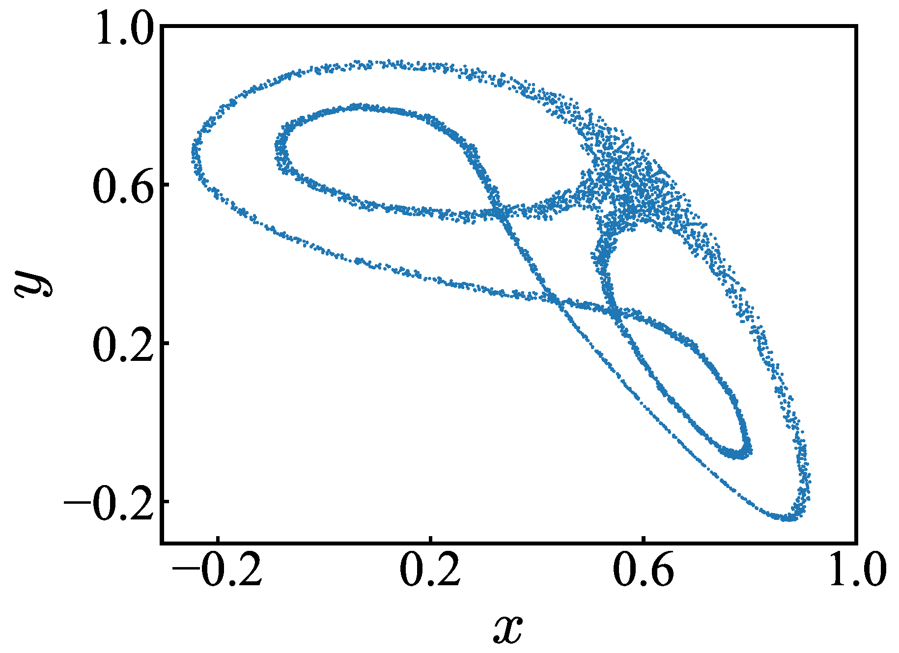
The parameters are fixed as $a=0.01$, $b=0.8$, $c=0.99$, for which the discrete 3D sinusoidal map exhibits chaotic behavior [31]. The system demonstrates chaos due to its nonlinear terms and strong sensitivity to initial conditions. These properties make it an excellent candidate for reservoir computing since its non-linear nature and chaotic behavior enable it to respond uniquely to small changes in input. The complexity of its dynamics ensures it can capture temporal patterns. The inclusion of sine functions adds to its complexity, enriching its dynamics. In this paper, an individual reservoir node is modeled, and its synchronization with another identical system with linear coupling is investigated. The 3D sinusoidal map shows a discrete Lorenz-type attractor where the topology is similar to that of the continuous Lorenz attractor generated by the 3D continuous Lorenz system; note that the terms of the 3D sinusoidal map are not similar to those of the 3D Lorenz flow system (see Figure 3). This makes the system well-suited for studying synchronization in coupled reservoir computing frameworks.

To examine the effect of coupling strength on synchronization, we analyzed the synchronization error ($\Delta$) between two coupled reservoir computers for 100 uniformly spaced values of coupling strength $\alpha$ in the range [0, 1]. The experiments were repeated over 10 independent trials by following the procedure outlined in Algorithm 1. 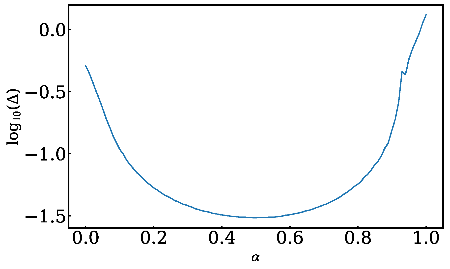The mean of the synchronization errors is taken over the 10 trials at each $\alpha$ and the results are presented in Figure 4. The minimum error is observed near ${\alpha }_{min}=0.525$, indicating that this value corresponds to the optimal coupling strength for synchronization.

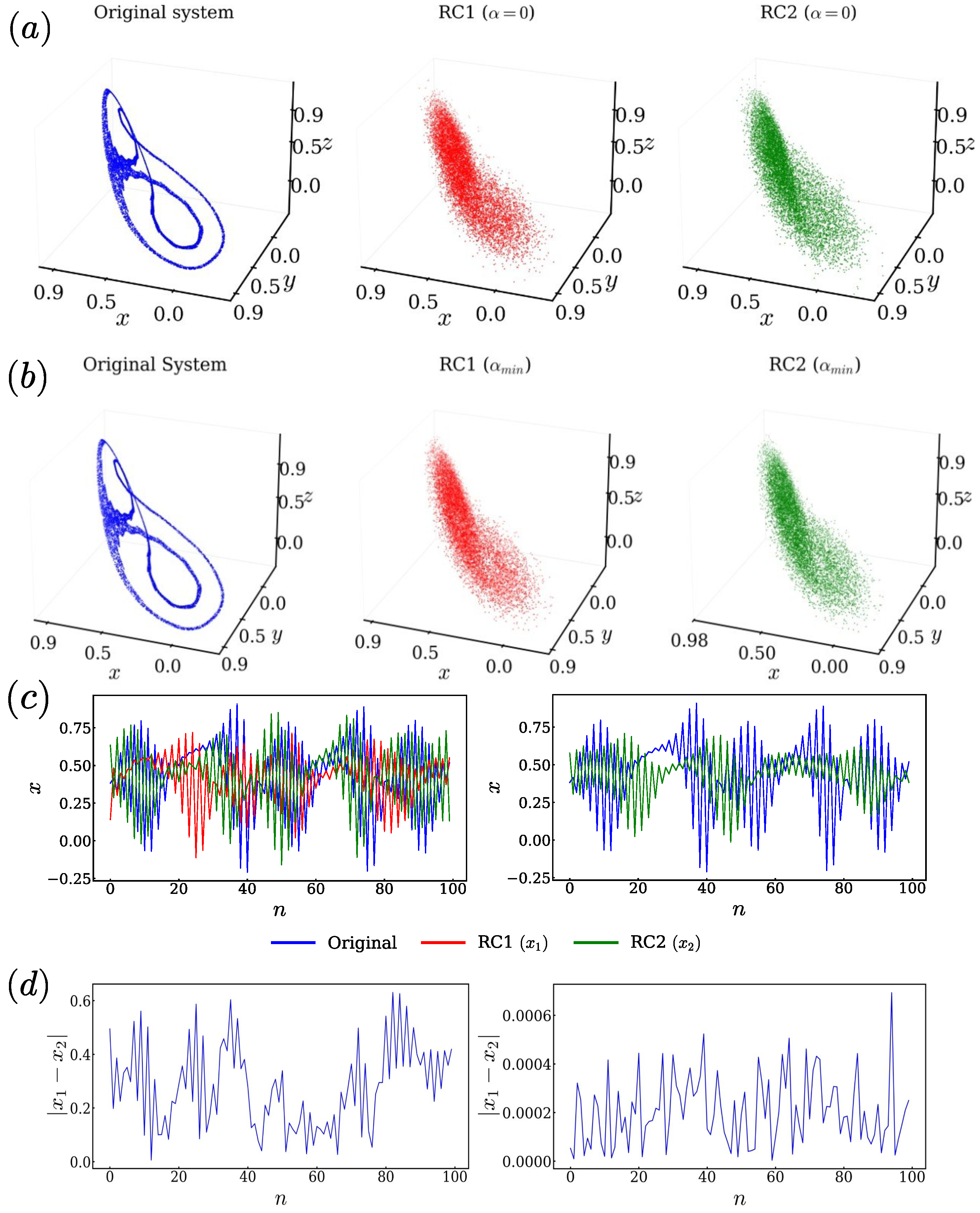
In Figure 5a and Figure 5b, we present the phase portraits of the two reservoirs coupled with coupling strength $\alpha ={\alpha }_{min}$ and $\alpha =0$, respectively. $\alpha =0$ represents the fully autonomous (closed-loop) regime, in which the trained reservoirs RC1 and RC2 evolve independently without coupling, with each reservoir using only its own output as input for the next time step. Figure 5c,d show the corresponding time series plot where we have plotted $x_1$ and $x_2$ for the last 100 time steps in the same trial. From the time series plot, This confirms that synchronization is achieved under optimal coupling conditions at $\alpha ={\alpha }_{min}$, whereas no synchronization is observed in the uncoupled case at $\alpha =0$.

Following the analysis of the discrete 3D sinusoidal map with the discrete Lorenz attractor, we next examine the synchronization behavior of the 3D sinusoidal map with a conjoined Lorenz twin attractor (see Figure 6).

4.2. 3D Sinusoidal Map with Conjoined Lorenz Twin Attractor

We consider a three-dimensional discrete-time nonlinear map defined as

$$\begin{array}{cc}\hfill x_{n+1}& =y_n,\hfill \\ \hfill y_{n+1}& =sin\left(z_n\right),\hfill \\ \hfill z_{n+1}& =A{z}_n+B{x}_n+C{y}_n+Dsin\left(z_n{y}_n^2\right)+2z_n^3,\hfill \end{array}$$

(11)

where $x_n$, $y_n$, and $z_n$ denote the state variables at discrete time n, and $A,B,C,D\in \mathbb{R}$ are control parameters [32].

The map combines linear coupling with nonlinear sinusoidal and cubic terms, leading to a wide variety of dynamical behaviors, including periodic, quasiperiodic, and chaotic regimes. Owing to its invariance under the transformation $(x,y,z)\mapsto (-x,-y,-z)$, the system exhibits central symmetry, which gives rise to characteristic double-lobed conjoined discrete Lorenz attractors. In [32], various routes to the formation of discrete conjoined Lorenz twin attractors are discussed. Note that the terms of the 3D sinusoidal discrete map are not similar to that of the 3D Lorenz flow system.

The generated three-dimensional time series $\mathbf{u}\left(t\right)={[x\left(t\right),y\left(t\right),z\left(t\right)]}^{\top }$ is used as input for the reservoir computing framework.

We trained the reservoir computers using the proposed 3D sinusoidal map with conjoined Lorenz twin attractor and evaluated the synchronization error $\Delta$ as a function of the coupling strength $\alpha$. For $\alpha =0$, the reservoirs evolve independently, resulting in a relatively large synchronization error. As $\alpha$ increases, the coupling facilitates information exchange between the reservoirs, leading to a rapid initial reduction followed by a gradual decrease in the synchronization error (see Figure 7). The decrease in $\Delta$ is not strictly monotonic; small fluctuations are observed due to the inherent nonlinear and chaotic dynamics of the system. The synchronization error reaches a minimum around $\alpha \approx 0.6$, indicating the regime of strongest synchronization between the reservoirs. For larger values of $\alpha$, the error increases again, suggesting that excessive coupling disrupts the intrinsic reservoir dynamics and reduces synchronization accuracy.

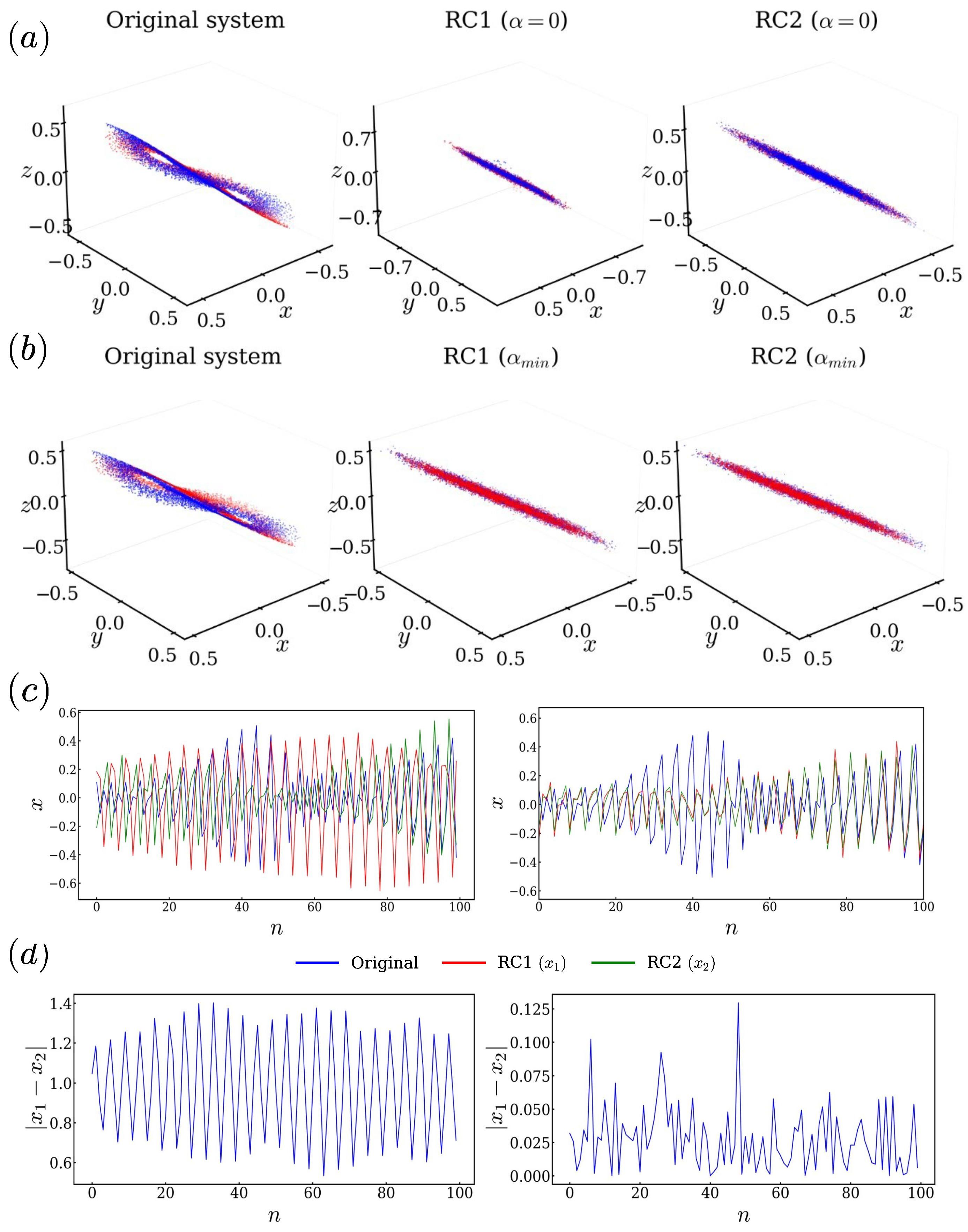
In Figure 8a,b, we present the phase portraits of the original attractor and the corresponding reservoir systems under two coupling conditions, $\alpha =0$ and $\alpha ={\alpha }_{min}$, respectively. When $\alpha =0$, the two reservoirs evolve independently, leading to visibly distinct trajectories. In contrast, at $\alpha ={\alpha }_{min}$, the phase portraits of the reservoirs closely overlap, indicating the emergence of synchronization. Figure 8c illustrates the corresponding time series of the state variables $x_1$ and $x_2$, along with the original system, over the last 100 time steps of the same trial. It can be observed that for $\alpha ={\alpha }_{min}$, the trajectories of $x_1$ and $x_2$ nearly coincide, demonstrating strong synchronization. However, for $\alpha =0$, a clear mismatch between the time series is evident, indicating desynchronization. Further quantitative evidence is provided in Figure 8d, which shows the absolute synchronization error $|x_1-x_2|$ over the final 100 time steps. For $\alpha ={\alpha }_{min}$, the error remains close to zero, confirming synchronized behavior. In contrast, for $\alpha =0$, the error exhibits significant fluctuations, highlighting the absence of synchronization.

Following the analysis of the 3D sinusoidal map with a conjoined Lorenz twin attractor, we next examine the synchronization behavior of the 3D quadratic hyperchaotic map.

4.3. 3D Quadratic Hyperchaotic Map

A 3D quadratic hyperchaotic map is defined by

$$\begin{array}{cc}\hfill x_{n+1}& =a_1{y}_n+a_2{y}_n^2,\hfill \\ \hfill y_{n+1}& =b_1-b_2{z}_n,\hfill \\ \hfill z_{n+1}& =c{x}_n,\hfill \end{array}$$

(12)

with fixed parameters $a_1=0.25$, $a_2=0.12$, $b_1=4$, $b_2=1.2$ and $c=2.15$ [33].

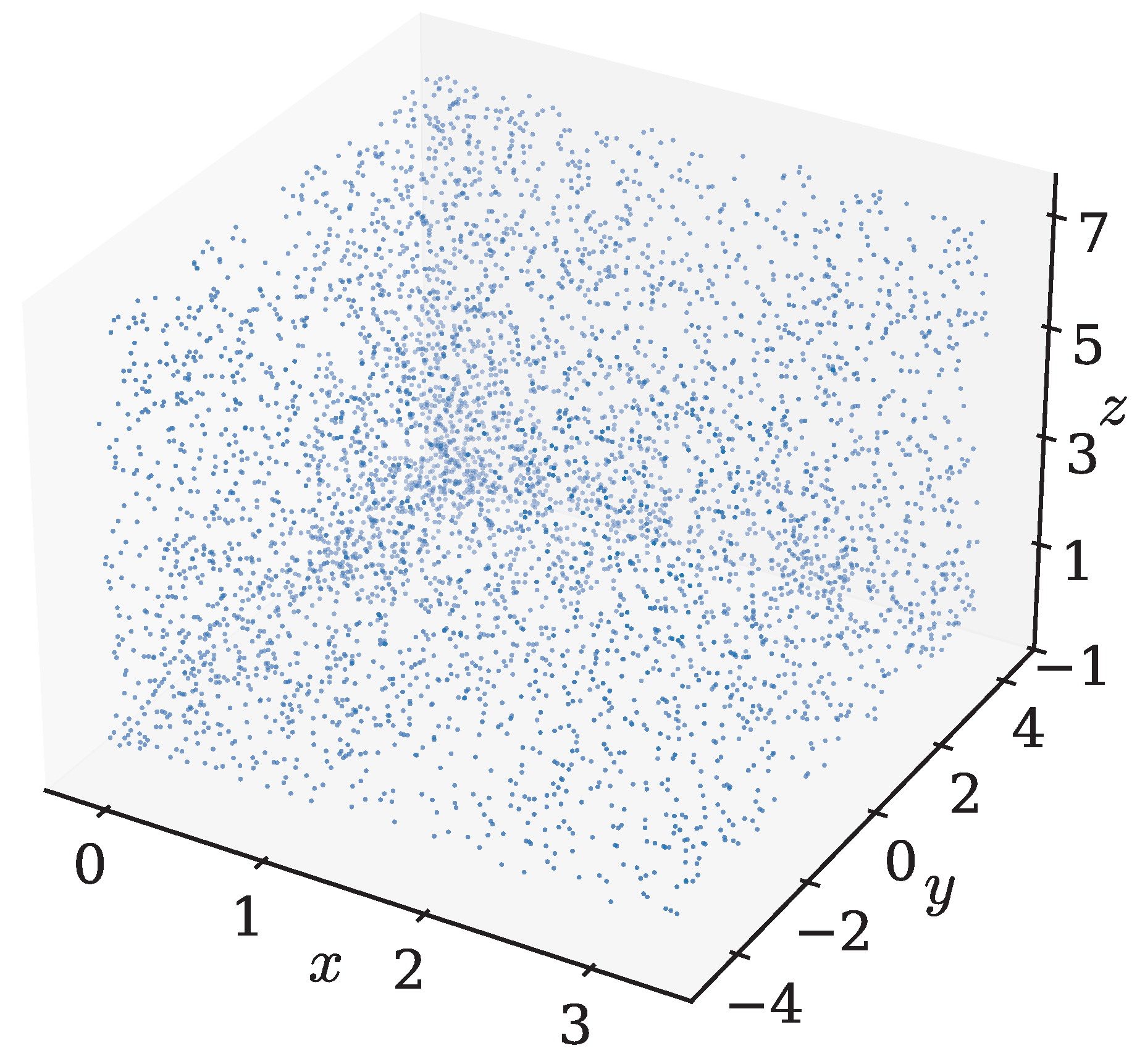
Figure 9 shows a three-dimensional phase plot of a hyperchaotic attractor. The three axes in the plot are labeled x, y, and z, indicating the state of the system at a given parameter set. In this case, the attractor exhibits hyperchaotic behavior with all three Lyapunov exponents. This indicates that they are extremely sensitive to initial conditions, and small variations at the outset can yield different results [23]. That is why the points in the plot appear scattered and spread out over a large area, rather than forming a simple shape like a loop or spiral. This hyperchaotic attractor looks cubic because it spreads uniformly in all directions (x, y, z). The ability of the reservoir computer to reproduce this hyperchaotic attractor indicates that it has successfully learned the behavior. This indicates that the model is not only able to predict future events but also to model the system’s long-term behavior. It has successfully learned and reproduced the complex, chaotic behavior of the original hyperchaotic system.

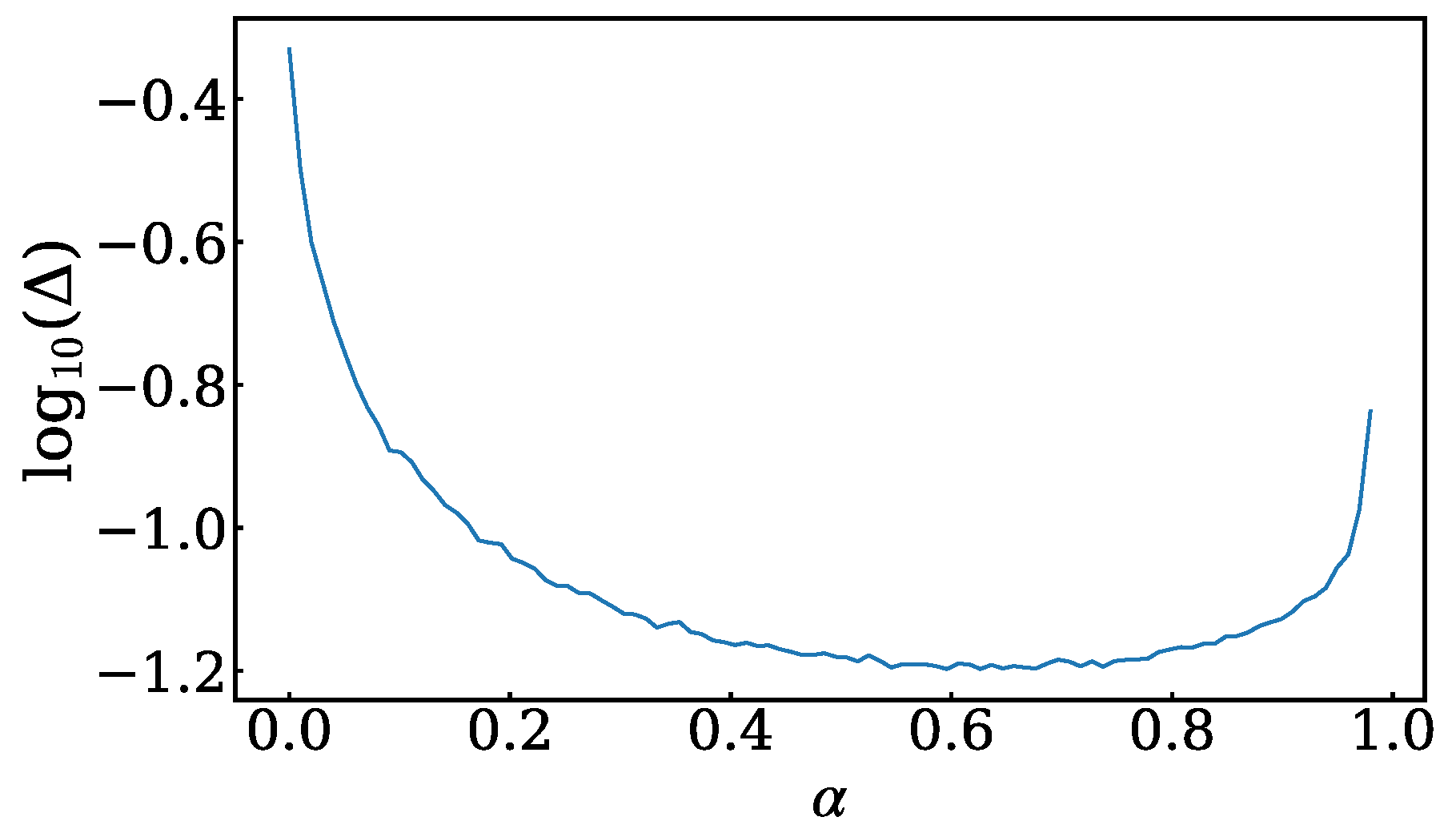
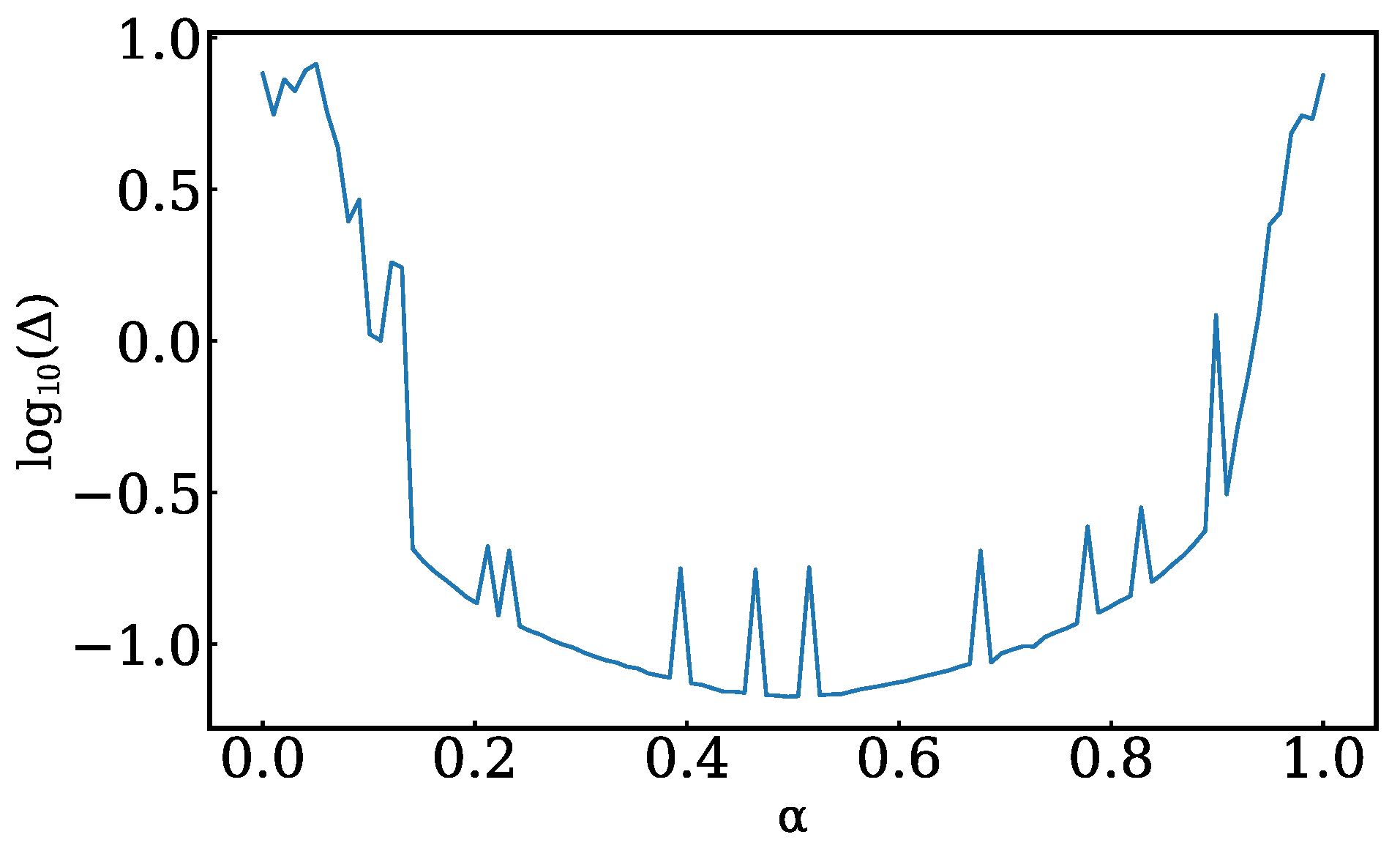
Figure 10 shows the synchronization error as we vary the coupling strength $\alpha$ between the reservoir computers [25]. The coupling strength $\alpha$ is a value between 0 and 1 that determines the strength of coupling between the two systems. For values of $\alpha$ close to zero, the coupling is weak, and the reservoirs evolve almost independently, resulting in a large synchronization error. As $\alpha$ is increased, the coupling between the two systems becomes stronger, leading to a reduction in the synchronization error. An optimal synchronization regime is observed for intermediate coupling strengths, where the synchronization error attains its minimum value. In this regime, although the two reservoir computers exhibit a high degree of synchronization, the synchronization error is not 0. This behavior is expected due to the hyperchaotic nature of the underlying system. In hyperchaotic systems, perfect synchronization is generally unattainable, even under strong coupling. As the coupling strength is further increased toward $\alpha =1$, the synchronization error increases again, indicating a degradation of synchronization at very strong coupling. Overall, the synchronization error exhibits a characteristic U-shaped dependence on $\alpha$ with poor synchronization at both very weak and very strong coupling.

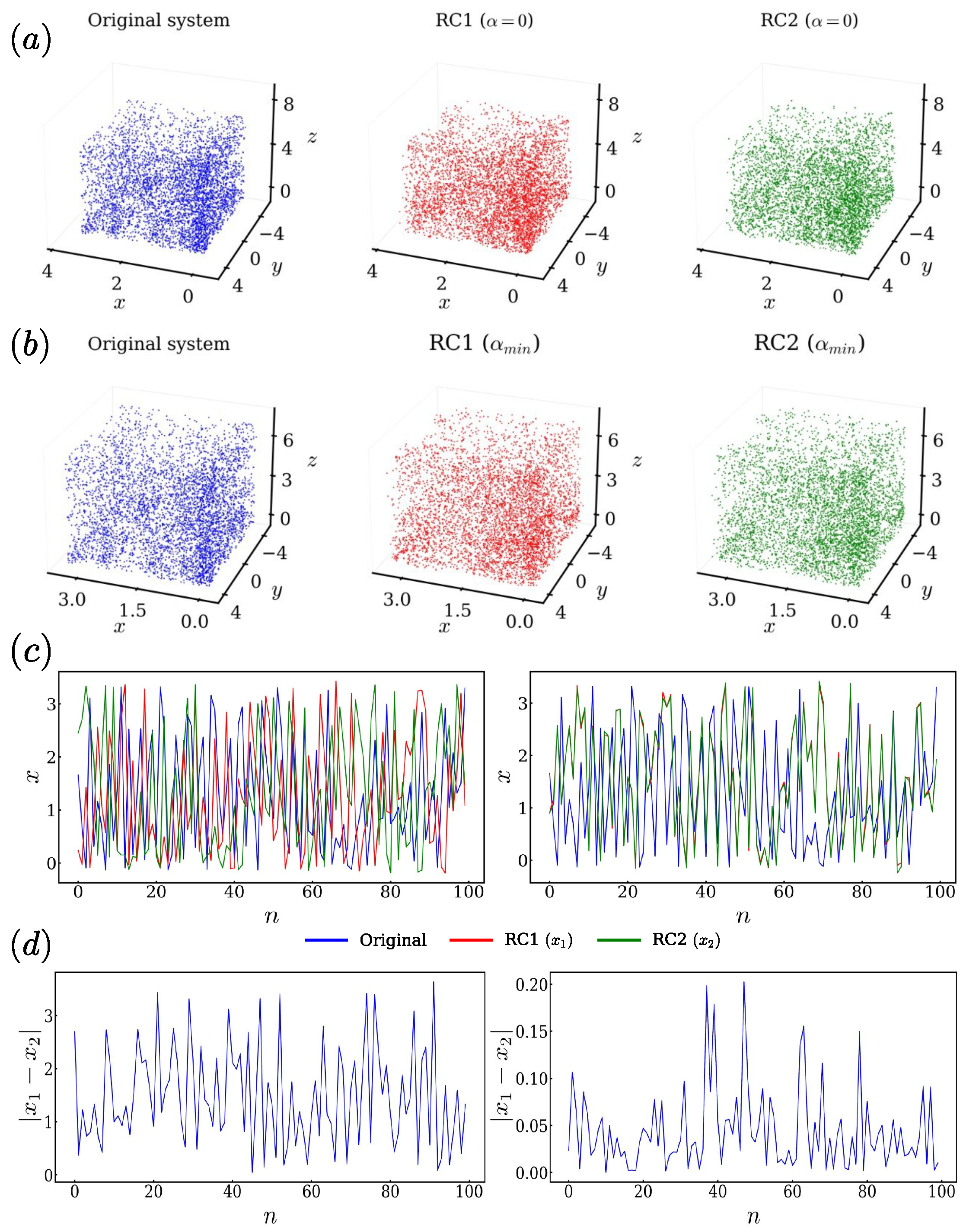
In Figure 11a and Figure 11b, we present the phase portraits of the two reservoirs coupled with coupling strengths $\alpha =0$ and $\alpha ={\alpha }_{min}$, respectively. Figure 11c,d show the corresponding time series plots, where we have plotted $x_1$ and $x_2$ for the last 100 time steps of the same trial. From the time series plots, we can clearly see that the two reservoir computers are closely synchronized at coupling strength ${\alpha }_{min}$, but not closely synchronized when operated at coupling strength 0.

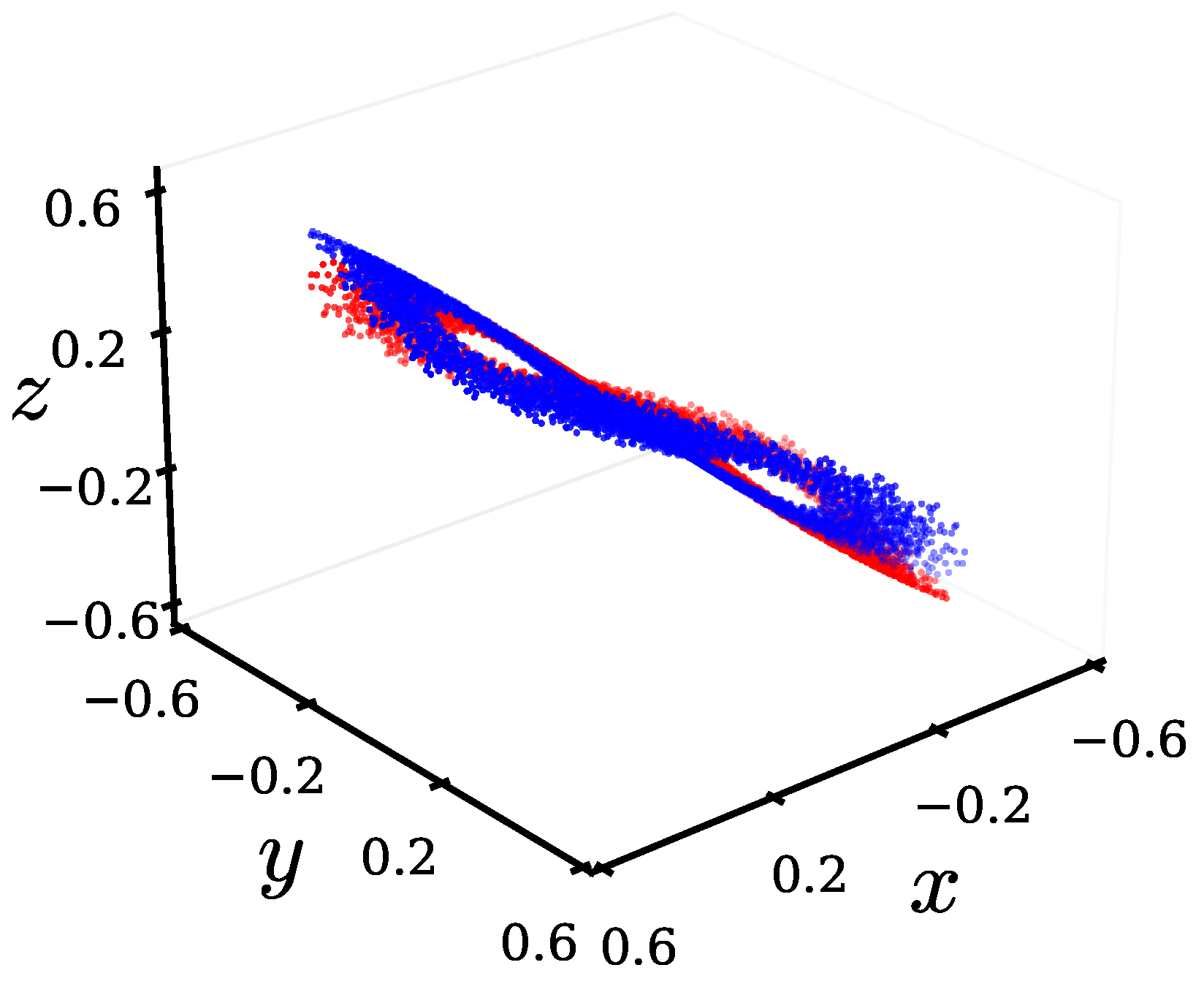
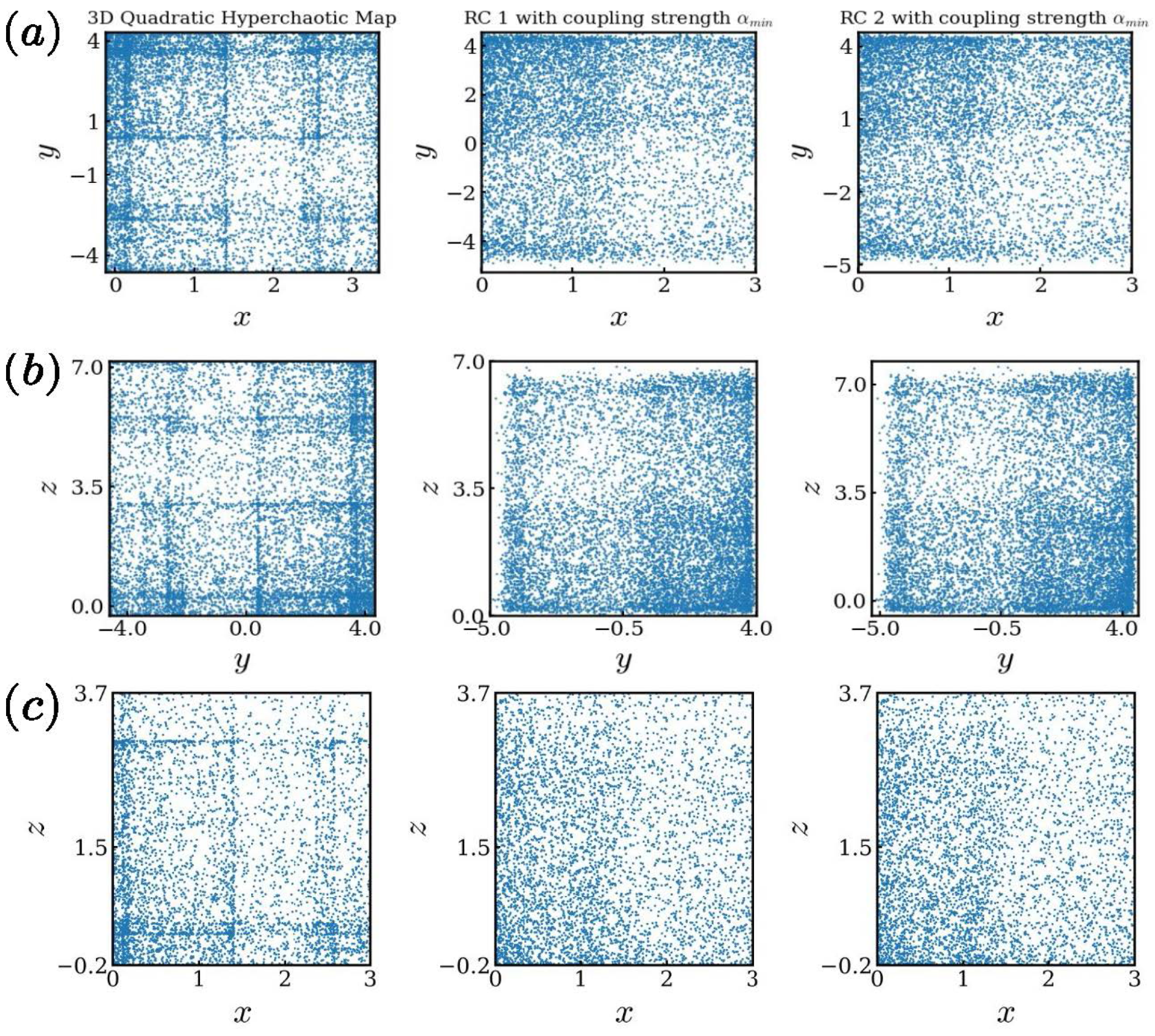
Figure 12 presents the two-dimensional projections of the phase portraits for the original system and the corresponding reservoir computers under symmetric coupling at $\alpha ={\alpha }_{min}$. Specifically, Figure 12a–c show the projections onto the x–y, y–z, and x–z planes, respectively. In each row, the left panel corresponds to the original system, while the middle and right panels show the outputs of RC1 and RC2, respectively. It can be observed that the projected attractor structures of both reservoirs closely resemble that of the original system across all three planes. The strong overlap in geometric structures indicates that the reservoirs can accurately reconstruct the underlying attractor dynamics. Moreover, the close agreement between the projections of RC1 and RC2 confirms that the two reservoirs are well synchronized under the chosen coupling strength. These results demonstrate that symmetric linear coupling at $\alpha ={\alpha }_{min}$ enables the reservoir computers not only to learn the intrinsic dynamics of the system but also to maintain coherent synchronized behavior across multiple state-space projections.

5. Comparative Analysis of Synchronization Behavior

Table 1 provides a comparative overview of different reservoir computing approaches used for modeling and synchronization of chaotic systems. The comparison is based on key characteristics, including dependence on external input, coupling structure, level of autonomy, and the primary objective of each method. Reservoir computing approaches with external driving, such as Chua’s circuit-based model, rely on continuous input signals from the underlying chaotic system. In these methods, the reservoir is driven by the external time series, and the primary objective is accurate prediction of system dynamics rather than synchronization between independent systems. Consequently, these approaches do not exhibit autonomous behavior or mutual interaction between multiple reservoirs. master–slave reservoir computing synchronization methods extend this framework by introducing a unidirectional coupling mechanism, where a slave reservoir is driven by a master system. While synchronization is achieved in this setting, it is externally enforced through continuous input signals and a hierarchical structure. This limits the applicability of such methods in decentralized scenarios, as the slave system depends on the master for synchronization.

Coupled reservoir computing approaches with input-driven representation constitute a more advanced class of methods in which multiple reservoirs are interconnected and share information via transmitted or common input signals. Although partial coupling is present, these systems still depend on external inputs to maintain synchronization. As a result, the reservoirs do not operate in a fully autonomous manner, and synchronization remains input-driven rather than emerging intrinsically from the system dynamics. In contrast, the proposed method eliminates the need for external input after the training phase and does not rely on a master–slave configuration. The two reservoir computers operate autonomously and interact solely through symmetric mutual coupling. This enables synchronization to emerge from the interaction between independently learned dynamical systems. The primary objective of the proposed framework is therefore autonomous synchronization, which represents a fundamental shift from externally driven synchronization toward interaction-induced synchronization in reservoir computing systems.

The present work introduces a novel synchronization framework based on autonomously operating reservoir computers with symmetric linear coupling. The primary objective is to establish the feasibility of synchronization in this setting and to demonstrate its effectiveness across different chaotic systems. Accordingly, this study is intended as a proof-of-concept rather than a comprehensive performance comparison with existing synchronization methods. A systematic evaluation against the above classical approaches, in terms of synchronization error, convergence rate, and robustness, constitutes an important direction for future research.

Table 5. Quantitative comparison of synchronization performance across different chaotic systems.

System	${\mathsf{\Delta }}_{\mathit{min}}$	${\mathit{\alpha }}_{\mathit{min}}$	Trend
Discrete 3D sinusoidal map with discrete Lorenz attractor	$0.0279\pm 0.0032$	∼0.5	U-shaped
3D sinusoidal map with conjoined Lorenz twin attractor	$0.0601\pm 0.0019$	∼0.6	U-shaped
3D quadratic hyperchaotic map	$0.0683\pm 0.0058$	∼0.5	U-shaped

summarizes the synchronization performance of the reservoir-based framework across three representative discrete chaotic systems. For all systems considered, the synchronization error $\Delta$ exhibits a pronounced U-shaped dependence on the coupling strength $\alpha$, with the minimum error consistently occurring near $\alpha \approx 0.5$.

Among the systems studied, the discrete 3D sinusoidal map with discrete Lorenz attractor achieves the lowest minimum synchronization error, ${\Delta }_{min}=0.0279\pm 0.0032$, indicating superior synchronization performance. In contrast, the 3D sinusoidal map with a conjoined Lorenz twin attractor and the 3D quadratic hyperchaotic map exhibit higher minimum synchronization errors, with ${\Delta }_{min}=0.0601\pm 0.0019$ and ${\Delta }_{min}=0.0683\pm 0.0058$, respectively. Nevertheless, all systems maintain synchronization over a wide range of coupling strengths, approximately from $\alpha =0.1$ to $\alpha =0.9$.

6. Conclusions

This work investigates the use of reservoir computing for learning and reproducing the dynamics of chaotic systems, with particular emphasis on synchronization between independently trained reservoirs. In this work, a simple symmetric linear coupling was used to couple the two independently trained reservoir computers. The use of linear coupling is motivated by its simplicity and by the objective of determining whether a simple linear coupling mechanism can facilitate synchronization between reservoir computers trained on chaotic and hyperchaotic systems. Three representative discrete-time chaotic and hyperchaotic systems were examined, namely, a discrete sinusoidal map, a 3D sinusoidal map with a conjoined Lorenz twin attractor, and a quadratic hyperchaotic map. For all systems considered, the synchronization error $\Delta$ exhibited a characteristic U-shaped dependence on the coupling strength $\alpha$. As $\alpha$ was increased from zero, the synchronization error initially decreased, reaching a minimum near $\alpha \approx 0.5$, and subsequently increased for larger coupling values. This behavior indicates the existence of an optimal intermediate coupling regime that maximizes synchronization while preserving chaotic dynamics. At low coupling strengths, the reservoirs evolved independently, whereas excessively strong coupling alters the dynamical behavior and leads to increased synchronization error, indicating a degradation of collective dynamical coherence rather than stable synchronization.

For the 3D sinusoidal map, the synchronization behavior exhibits a clear dependence on the coupling strength $\alpha$. The synchronization error $\Delta$ decreases as $\alpha$ increases, reaching a minimum at an intermediate value of $\alpha$, beyond which the error increases again. This indicates the existence of an optimal coupling regime that balances interaction strength and dynamical coherence. Compared to more sensitive systems, the sinusoidal map demonstrates relatively stable synchronization over a wider range of coupling strengths, with only mild variations in synchronization error. Synchronization performance is quantified using the average synchronization error $\Delta$, supported by qualitative agreement observed in phase portrait overlap and output time series. The trained reservoir computers successfully reproduce the geometric structure of the underlying chaotic attractor and achieve consistent synchronization under appropriate coupling conditions. However, as expected for chaotic systems, accurate dynamical reproduction is primarily limited to short time horizons due to sensitivity to initial conditions. These results demonstrate effective learning of the system dynamics while acknowledging the inherent limitations of long-term prediction in chaotic regimes.

Synchronizing reservoir computers makes it possible for multiple autonomous, data-driven models to work together in a coordinated way without relying on centralized control. This is particularly useful in practical settings such as distributed sensing, cooperative prediction, and secure communication, where reliable and consistent behavior must emerge from decentralized systems. The present study is limited to discrete-time three-dimensional chaotic and hyperchaotic systems and considers a simple symmetric linear coupling mechanism. Future work may extend this framework to continuous-time systems and higher-dimensional dynamics. Exploring non-linear, adaptive, or time-varying coupling mechanisms also remains an important direction for future research.

References

- Lukoševičius, M.; Jaeger, H. Reservoir computing approaches to recurrent neural network training. Comput. Sci. Rev. 2009, 3, 127–149. [Google Scholar] [CrossRef]
- Zuo, Z.; Cao, R.; Gan, Z.; Hou, J.; Guan, C.; Leng, S. Feedback coupling induced synchronization of neural networks. Neurocomputing 2023, 549, 126457. [Google Scholar] [CrossRef]
- Zhao, L.; Sun, Z.; Tang, M.; Guan, S.; Zou, Y. Learning successive weak synchronization transitions and coupling directions by reservoir computing. Chaos Solitons Fractals 2023, 168, 113139. [Google Scholar] [CrossRef]
- Tanaka, G.; Yamane, T.; Héroux, J.B.; Nakane, R.; Kanazawa, N.; Takeda, S.; Numata, H.; Nakano, D.; Hirose, A. Recent advances in physical reservoir computing: A review. Neural Netw. 2019, 115, 100–123. [Google Scholar] [CrossRef] [PubMed]
- Parlitz, U. Learning from the past: Reservoir computing using delayed variables. Front. Appl. Math. Stat. 2024, 10, 1221051. [Google Scholar] [CrossRef]
- Sato, Y.; Kobayashi, M.U. Minimal model for reservoir computing. Phys. D Nonlinear Phenom. 2024, 470, 134360. [Google Scholar] [CrossRef]
- Zhang, W.; Zhou, S.; Li, H.; Zhu, H. Chaos in a fractional order Rössler system. Chaos Solitons Fractals 2009, 42, 1684–1691. [Google Scholar] [CrossRef]
- Wikner, A.; Harvey, J.; Girvan, M.; Hunt, B.R.; Pomerance, A.; Antonsen, T.; Ott, E. Stabilizing machine learning prediction of dynamics: Novel noise-inspired regularization tested with reservoir computing. Neural Netw. 2024, 170, 94–110. [Google Scholar] [CrossRef]
- Kong, L.W.; Brewer, G.A.; Lai, Y.C. Reservoir-computing based associative memory and itinerancy for complex dynamical attractors. Nat. Commun. 2024, 15, 4840. [Google Scholar] [CrossRef]
- Bezruchko, B.P.; Ponomarenko, V.I.; Smirnov, D.A.; Sysoev, I.V.; Prokhorov, M.D. Class-oriented techniques for reconstruction of dynamics from time series. Chaos Solitons Fractals 2021, 148, 110972. [Google Scholar] [CrossRef]
- Momani, S.; Batiha, I.M.; Bendib, I.; Ouannas, A.; Hioual, A.; Mohamed, D. Examining finite-time behaviors in the fractional Gray–Scott model: Stability, synchronization, and simulation analysis. Int. J. Cogn. Comput. Eng. 2025, 6, 380–390. [Google Scholar] [CrossRef]
- Mori, Y.; Kawada, T.; Fukuda, S.; Gotoda, H. Nonlinear dynamics of attenuation behavior in combustion oscillations in a swirl-stabilized combustor. Proc. Combust. Inst. 2023, 39, 4671–4679. [Google Scholar] [CrossRef]
- Ma, R.; Dai, Q.; Li, H.; Yang, J. Dynamics reconstruction in the presence of bistability by using reservoir computer. Chaos Solitons Fractals 2023, 172, 113523. [Google Scholar] [CrossRef]
- Mahata, A.; Kingston, S.L.; Ghosh, S.; Dana, S.K.; Kapitaniak, T. Learning transitions to extreme events using reservoir computing. Phys. Rev. E 2025, 112, 054207. [Google Scholar] [CrossRef]
- Mochiutti, E.; Antonelo, E.A.; Camponogara, E. Physics-informed Echo State Networks for modeling controllable dynamical systems. Neurocomputing 2025, 639, 130251. [Google Scholar] [CrossRef]
- Cheng, J.; Gao, T.; Duan, J. Adaptive control for multi-scale stochastic dynamic systems with stochastic next generation reservoir computing. Phys. D Nonlinear Phenom. 2026, 492, 135206. [Google Scholar] [CrossRef]
- Minati, L.; Li, C.; Bartels, J.; Chakraborty, P.; Li, Z.; Yoshimura, N.; Frasca, M.; Ito, H. Accelerometer time series augmentation through externally driving a non-linear dynamical system. Chaos Solitons Fractals 2023, 168, 113100. [Google Scholar] [CrossRef]
- Antonik, P.; Gulina, M.; Pauwels, J.; Massar, S. Using a reservoir computer to learn chaotic attractors, with applications to chaos synchronization and cryptography. Phys. Rev. E 2018, 98, 012215. [Google Scholar] [CrossRef]
- Pecora, L.M.; Carroll, T.L. Synchronization in chaotic systems. Phys. Rev. Lett. 1990, 64, 821. [Google Scholar] [CrossRef]
- Weng, T.; Song, J.; Yang, H.; Gu, C.; Zhang, J.; Small, M. Synchronization of reservoir computers with applications to communications. Phys. A Stat. Mech. Its Appl. 2020, 544, 123453. [Google Scholar] [CrossRef]
- Lun, S.; Sun, Z.; Li, M.; Wang, L. Multiple-Reservoir Hierarchical Echo State Network. Mathematics 2023, 11, 3961. [Google Scholar] [CrossRef]
- Liu, J.; Zhang, J.; Wang, Y. Secure communication via chaotic synchronization based on reservoir computing. IEEE Trans. Neural Netw. Learn. Syst. 2024, 35, 285–299. [Google Scholar] [CrossRef] [PubMed]
- Hu, W.; Zhang, Y.; Ma, R.; Dai, Q.; Yang, J. Synchronization between two linearly coupled reservoir computers. Chaos Solitons Fractals 2022, 157, 111882. [Google Scholar] [CrossRef]
- dos Santos, A.M.; Viana, R.L.; Lopes, S.R.; de S. Pinto, S.E.; Batista, A.M. Collective behavior in coupled chaotic map lattices with random perturbations. Phys. A Stat. Mech. Its Appl. 2008, 387, 1655–1668. [Google Scholar] [CrossRef]
- West, B.J.; Geneston, E.L.; Grigolini, P. Maximizing information exchange between complex networks. Phys. Rep. 2008, 468, 1–99. [Google Scholar] [CrossRef]
- Liu, X.; Liu, B.; Guan, G. High-accuracy prediction of chaotic time series using multi-stage coupled Chua’s circuit-based reservoir computing. Neurocomputing 2026, 672, 132867. [Google Scholar] [CrossRef]
- Pyragas, K.; Pyragienė, T. Developing reservoir computing models for anticipatory synchronization with chaotic time series and real-time prediction. Phys. Rev. E 2025, 112, 015301. [Google Scholar] [CrossRef]
- Wyffels, F.; Schrauwen, B.; Stroobandt, D. Stable Output Feedback in Reservoir Computing Using Ridge Regression. In Artificial Neural Networks—ICANN 2008; Springer: Berlin/Heidelberg, Germany, 2008; pp. 808–817. [Google Scholar] [CrossRef]
- Jade, A.; Srikanth, B.; Jayaraman, V.; Kulkarni, B.; Jog, J.; Priya, L. Feature extraction and denoising using kernel PCA. Chem. Eng. Sci. 2003, 58, 4441–4448. [Google Scholar] [CrossRef]
- Bollobás, B. The evolution of random graphs. Trans. Am. Math. Soc. 1984, 286, 257–274. [Google Scholar] [CrossRef]
- Muni, S.S. Discrete Lorenz Attractors in 3D Sinusoidal Maps. Int. J. Bifurc. Chaos 2026, 36, 2630002. [Google Scholar] [CrossRef]
- Muni, S.S. Conjoined Lorenz twin attractors in 3D sinusoidal map. Chaos Solitons Fractals 2026, 206, 117894. [Google Scholar] [CrossRef]
- Muni, S.S. Pathways to hyperchaos in a three-dimensional quadratic map. Eur. Phys. J. Plus 2024, 139, 636. [Google Scholar] [CrossRef]
Figure 1.
Flowchart illustrating the key steps in the reservoir computing framework for synchronizing two reservoir computers. The process includes system setup, training, coupling, and error analysis to identify optimal synchronization conditions.
Figure 2.
Schematic representation of the reservoir computing architecture. The input signal is mapped into a high-dimensional reservoir through the input weight matrix . The reservoir consists of N sparsely connected nodes with internal weight matrix A (reservoir weights), producing a state vector . The output is obtained by applying a trained linear readout to the reservoir states.
Figure 3.
Phase portrait of the discrete-time 3D sinusoidal map defined by Equation (
10) with parameters
,
, and
. The plot illustrates the dense, double-lobed attractor produced by the discrete 3D sinusoidal map.
Figure 4.
Mean synchronization error over 10 trials versus coupling strength for the non-linear discrete-time 3D sinusoidal map. As the coupling strength increases, the synchronization error decreases, reaching a minimum near , before it increases again.
Figure 5.
In (a) and (b), depict the phase portraits of the two reservoirs coupled with coupling strengths and , respectively. (c) shows the corresponding time series, together with the time series of the original attractor, for the last 100 time steps of the same trial. (d) shows the corresponding absolute difference in the x-components of RC1 and RC2, , over the final 100 time steps for the same trial.
Figure 6.
Phase portrait of the 3D sinusoidal map with conjoined Lorenz twin attractor (Equation (
11)) for parameter
, showing chaotic attractor in
plane.
Figure 7.
Variation in synchronization error () over 10 trials with respect to coupling strength () in a 3D sinusoidal map with conjoined Lorenz twin attractor. The plot exhibits a characteristic U-shaped dependence on , where the error decreases initially, attains a minimum at an intermediate coupling strength, and increases again for larger .
Figure 8.
In (a) and (b), depict the phase portraits of the original attractor and two reservoirs coupled with coupling strengths and , respectively. (c) shows the corresponding time series, along with the time series of the original attractor, for the last 100 time steps of the same trial. (d) shows the corresponding absolute difference in the x-components of RC1 and RC2, , over the final 100 time steps for the same trial.
Figure 9.
3D phase portrait of the 3D quadratic hyperchaotic map (Equation (
12)) with parameters
. The trajectory forms a bounded cubic-shaped attractor in the
space, showing hyperchaotic behavior with all three positive Lyapunov exponents.
Figure 10.
Synchronization error vs. coupling strength plot of 3D hyperchaotic system. The best synchronization occurs between = 0.4 and 0.6. The U-shaped curve indicates that both weak and strong coupling lead to higher synchronization error.
Figure 11.
(a) and (b) show the phase portraits of the two reservoirs coupled with different coupling strengths and , respectively. (c) shows the corresponding time series, together with that of the original attractor, for the last 100 time steps of the same trial. (d) shows the corresponding absolute difference between the x-components of RC1 and RC2, , over the final 100 time steps for the same trial.
Figure 12.
Two-dimensional projections ((a) x–y, (b) y–z, and (c) x–z) of the phase portraits of the three-dimensional quadratic hyperchaotic map are presented for the original system (first column), and the outputs of RC1 (second column) and RC2 (third column) under symmetric coupling at . The strong overlap between the projections illustrates the ability of the trained reservoir computers to reproduce the attractor structure and achieve synchronization effectively under symmetric linear coupling.