Experimental Validation and Reservoir Computing Capability of Spiking Neuron Based on Threshold Selector and Tunnel Diode

Abstract

Despite the success of artificial neural networks in solving numerous tasks, they face significant challenges, including difficulties in online adaptation and rapidly increasing energy consumption. As a biologically plausible alternative, spiking neural networks offer promising capabilities for efficient cognitive computing. Recently, a three-element spiking neuron model consisting of a threshold selector, a tunnel diode, and a capacitor was proposed. In this work, we experimentally validate this model using a threshold selector hardware emulator and demonstrate its dynamical equivalence to the biologically plausible Izhikevich neuron model. To evaluate the novel neuron’s applicability for cognitive computing, we implement a liquid state machine (LSM) reservoir architecture with spatially dependent random topology for synaptic weight distribution. Our simulations on the MNIST and Fashion-MNIST benchmarks demonstrate competitive classification accuracy (97.9% and 89.5%, respectively) while offering estimated energy efficiency and processing speed enhancements compared to existing FPGA-based and memristor-based spiking reservoir implementations. The developed reservoir is feasible for processing neuromorphic sensors output, including visual perception tasks.

1. Introduction

1.1. Deep Learning Paradigm Issues, and Reservoir Computing as an Alternative

Artificial neural networks (ANNs) are currently used to solve a wide range of problems, including classification, recognition, data generation, and others [1]. Classical algorithms involve deterministic processing of input data based on predefined rules. In contrast, neural networks, during the training process, form their own internal model of information representation by identifying complex, non-obvious patterns in data. This allows them to be effectively applied to problems where providing an explicit, formalized description of the algorithm is difficult. However, the stable application of neural networks faces a number of obstacles, which include, in particular, the vanishing and exploding gradient problems that disrupt the learning process [2]. Other challenges include the ever-increasing energy consumption and computational resource requirements, directly linked to the growing size of models and the volume of data to be processed [3,4]. In this regard, one might argue that deep learning faces a paradigm crisis. A potential way out of this crisis is to turn to biologically more plausible neuron models, network architectures, and learning mechanisms.

Promising architectures include reservoir computing (RC). Reservoirs are a type of neural network with recurrent connections between neurons [5]. Their core idea is that only the output layers are trained, while the connections within the main body (the reservoir) are fixed and provide a high-dimensional separation of input data through nonlinearity and scale effects. In recent years, their effectiveness has been demonstrated in solving numerous practical problems. In particular, Morando et al. [6] used reservoir computing with automatic parameter optimization for fault diagnosis in proton exchange membrane fuel cells (PEMFCs), demonstrating the possibility of real-time diagnostics without changing the system’s operating conditions. Zhang et al. [7] used reservoir computing for fault diagnosis in 3D printers equipped with a low-cost position sensor.

1.2. Spiking Neural Networks: Motivation, Benefits from Reservoir Architecture, and Hardware Implementations

Artificial neuron models, first proposed by McCulloch and Pitts in 1943 [8], form the foundation of ANNs and are categorized into generations based on their operating principles. First-generation neurons employ a step activation function, limiting them to linearly separable problems, while the second generation overcame this constraint using continuous, nonlinear activation functions such as sigmoid or ReLU [9]. This advancement enabled complex multi-layer architectures and backpropagation-based training, forming the basis of modern deep learning networks.

The third generation is based on spiking neurons, which are the most biologically plausible as they replicate the dynamics of nervous tissue. Their operating principle is the exchange of discrete spikes (action potentials); the distribution of spikes over time allows encoding and processing of any information. Third-generation neurons also employ an activation mechanism: upon reaching a certain threshold of input stimulation, a spike is generated, after which the neuron’s potential resets, and a refractory period begins [10]. This time-dependent operational mechanism characterizes the system as dynamic, consequently providing the ability to work with time-varying data. However, this also introduces the requirement for fundamentally new training methods. Here, reservoir computing holds significant appeal: it does not require the training associated with adjusting the weights of synaptic connections within the reservoir, and the output layer can be implemented by any classifier, not necessarily one based on spiking neurons.

Key performance metrics for neural networks include their rate and energy consumption [11], which impose a set of requirements on the computing hardware used to implement the network [12]. Typically, instead of a central processing unit (CPU), a graphics processing unit (GPU) is used for neural network operations, as it can perform numerous parallel matrix operations. Alternatives to GPUs include tensor processing units (TPUs) or neural processing units (NPUs), which are designed in a similar way. However, all these accelerators face a fundamental limitation of von Neumann architecture: the need to transfer data between computational units, memory, and the central processor, which prevents fully asynchronous computation [13]. An alternative approach is represented by hardware architectures specifically designed for implementing hardware-based neural networks, known as neuromorphic architectures. In these systems, each neuron or group of neurons (in the case of time-multiplexed systems) is represented by a separate hardware module, interconnected with others in a multi-level structure [14]. This approach offers significantly higher speed and energy efficiency. Examples of such systems include the Intel Loihi [14] and IBM TrueNorth [15] neuroprocessors, and a number of FPGA implementations [16]. Even more promising in terms of energy efficiency, speed, and neuron density on a chip are neural networks implementing analog computations [13]. Emerging neuromorphic paradigms are increasingly considered for secure, data-driven applications where event-based processing and inherent physical unclonability offer advantages for privacy-preserving edge intelligence [17].

1.3. Analog Electronic Spiking Neurons: Brief Survey and Contribution of the Current Study

Recently, a number of compact models of biologically plausible analog neurons have been presented: based on a thyristor (SCR) [18,19], a uni-junction transistor (UJT) [20,21], as well as numerous models based on volatile memristors, also known as threshold selectors [22,23,24,25]. In the latter work [25], we propose a neuron model based on three elements: a threshold selector (TS), a tunnel diode, and a capacitor, along with two auxiliary voltage sources that modulate the neuron’s activity. This model is attractive due to its simplicity and rich dynamics, which encompass three classes of excitability according to Hodgkin [26] and the presence of chaotic regimes, whereas hardware neuron models based on a single TS are integrators (Hodgkin’s class 1). A drawback of this neuron is the use of non-standard elements: a promising argentum nano-dots selector (AND-TS) [27], which exists only as experimental prototypes, and legacy germanium tunnel diode. However, the fabrication of such elements or their counterparts in a chip is of fundamental possibility.

Putting together everything mentioned in this section, in the current study, we demonstrate for the first time the feasibility of the energy-efficient compact three-element analog spiking neuron for cognitive computing. In particular, the contribution and novelty of this work are as follows:

1.

We experimentally explore the hardware model of a neuron comprised of a threshold selector, a tunnel diode, and a capacitor, which was previously proposed in [25] only in simulation, and verify the validity of its mathematical model. In this model, we use a simplified threshold selector equation, feasible for analog hardware implementation.

2.

To evaluate the three-element neuron’s capability for cognitive computing, we develop a numerical model of a reservoir computer on its basis, following a liquid state machine (LSM) architecture with a recent biologically plausible spatially dependent random synaptic weight assignment algorithm [28]. To improve computational efficiency for numerical experiments via GPU, the three-element neuron model was replaced with the properly fitted Izhikevich model [29].

3.

Based on simulation results, we demonstrate its feasibility on benchmark classification problems by quantitatively evaluating its accuracy, performance, and energy efficiency.

2. Neuron Models

In this section, we propose experimental validation of the TS-TD neuron model and discuss its approximation by the Izhikevich neuron model for efficient numerical simulation.

2.1. Wilson Neuron and Three-Element Spiking Neuron

The core idea of the TS-TD neuron originates from circuit approximation of the simplified Hodgkin–Huxley model proposed by Wilson [30]. This model reveals the essential dynamical principles that allow action potential generation, while keeping the simplicity of FitzHugh–Nagumo neuron model, and is presented as follows:

$$\left\{\begin{array}{cc}C\dot{V}\hfill & =-g_{Na}\left(V\right)(V-E_{Na})-R(V-E_K)+I_{ext}\hfill \\ {\tau }_R\dot{R}\hfill & =-R+G\left(V\right)\hfill \end{array}\right.$$

(1)

In this system: V is the membrane potential (mV), R is a recovery variable representing slow potassium activation, C is the membrane capacitance (μF/cm²), $g_{Na}\left(V\right)$ is a voltage-dependent sodium-like conductance (mS/cm²), $E_{Na}$ and $E_K$ are sodium and potassium equilibrium potentials (mV), $I_{ext}$ is the externally injected current (μA/cm²), ${\tau }_R$ is the time constant of the recovery variable (ms), and $G\left(V\right)$ is the voltage-dependent steady-state function of the recovery variable. According to Wilson, $G\left(V\right)$ presents a linear function, while $g_{Na}\left(V\right)$ is best fitted by a quadratic polynomial, which, multiplied by the term $(V-E_{Na})$, forms the cubic $dV/dt$ isocline in a phase space.

The circuit model proposed by Ostrovskii et al. [25] is described by the equation of the similar structure:

$$\left\{\begin{array}{cc}C\dot{V}\hfill & =-I_{TD}(V-V_{TD})-G_M\left(x\right)·(V-V_M)+I_{ext}\hfill \\ \dot{x}\hfill & =f(V,x)\hfill \end{array}\right.$$

(2)

Here, V is a voltage on a membrane-imitating capacitor; threshold selector state variable x corresponds to recovery variable R in (1); external voltage sources $V_{TD}$ and $V_M$ replicate equilibrium potentials for sodium and potassium $E_{Na}$ and $E_K$, respectively; and $I_{TD}\left(y\right)$ is the tunnel diode current, which is roughly a cubic polynomial in shape, providing the negative differential resistance region essential for action potential generation [31]. Combined with the threshold selector, it enables three classes of excitability according to Hodgkin and chaotic regimes, distinguishing the TS-TD neuron from simple integrate-and-fire models. $G_M\left(x\right)$ is the threshold selector conductance, which stays mostly in two distinct states, namely the low-resistance state (LRS) and high-resistance state (HRS).

The mathematical model of the AND-TS device is presented in [25]. Here, keeping the original model dynamical features, we propose a novel simplified phenomenological AND-TS model based on smooth sigmoid-shape conductance transition between LRS and HRS driven by piecewise state variable x switching:

$$G_M\left(x\right)=K_1·arctan\left(\xi \pi (x-0.5)\right)+K_2$$

(3)

where

$$K_1={\displaystyle \frac{\pi G_{\mathrm{on}}}{\alpha }}$$

and

$$K_2=G_{\mathrm{off}}+{\displaystyle \frac{G_{\mathrm{on}}}{\alpha }}\left({\displaystyle \frac{{\pi }^2}{2}}-\beta \right).$$

The internal state has a piecewise voltage-driven drift:

$$\dot{x}=\left\{\begin{array}{cc}(1-x)\tau ,\hfill & V_M\ge V_{\mathrm{set}},\hfill \\ -x\tau ,\hfill & V_M\le V_{\mathrm{reset}}\hfill \end{array}\right.$$

LRS and HRS conductances $G_{\mathrm{on}}$ and $G_{\mathrm{off}}$, as well as set and reset voltages $V_{set}$ and $V_{reset}$, are parameters of the AND-TS device. The tunnel diode current is decomposed as

$$I_D\left(V\right)=I_{\mathrm{diode}}\left(V\right)+I_{\mathrm{tunnel}}\left(V\right)+I_{\mathrm{ex}}\left(V\right),$$

with

$$I_{\mathrm{diode}}\left(V\right)=I_s\left(exp\left({\displaystyle \frac{V}{V_t}}\right)-exp\left(-{\displaystyle \frac{V}{V_t}}\right)\right),$$

$$I_{\mathrm{tunnel}}\left(V\right)={\displaystyle \frac{I_p}{V_p}}Vexp\left(-{\displaystyle \frac{V-V_p}{V_p}}\right),$$

$$I_{\mathrm{ex}}\left(V\right)=I_v\left(arctan\left(D(V-E)\right)+arctan\left(D(V+E)\right)\right).$$

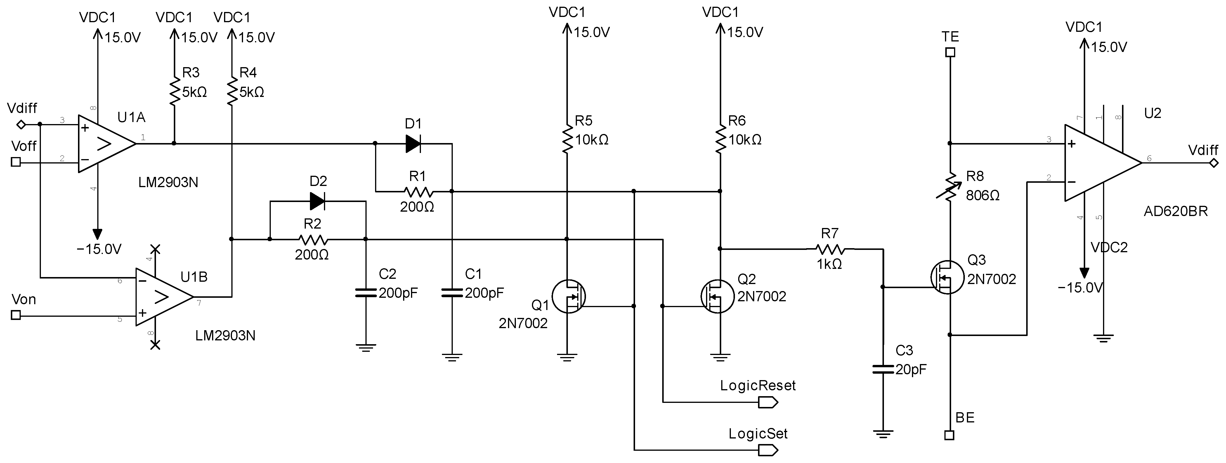
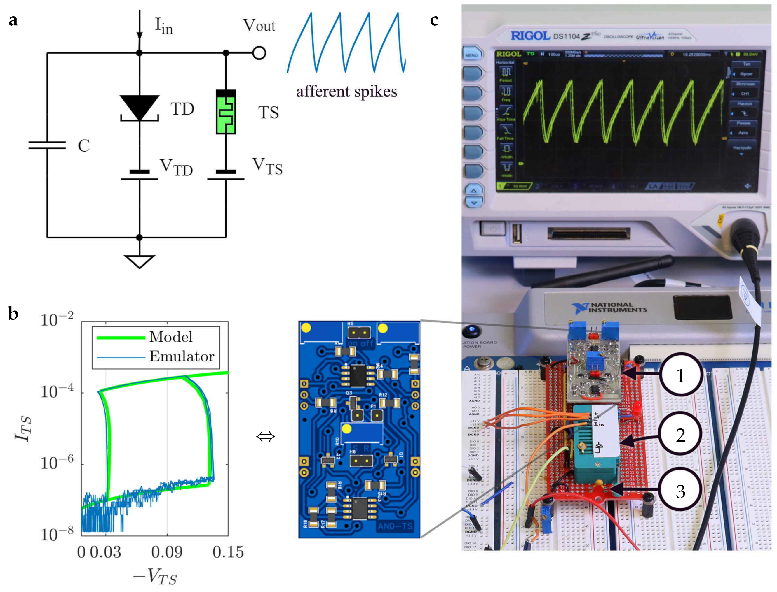
The numerical parameters of the TS-TD neuron model are presented in

Table 1. TS-TD neuron model parameters.

Symbol	Value	Description
$C_1$	$2.2\mathrm{nF}$	Membrane capacitance
$V_{\mathrm{on}}$	$0.119\mathrm{V}$	AND-TS set threshold
$V_{\mathrm{off}}$	$0.03\mathrm{V}$	AND-TS reset threshold
$R_{\mathrm{on}}$	$806\Omega$	AND-TS low-resistance state
$R_{\mathrm{off}}$	${10}^7\Omega$	AND-TS high-resistance state
$\xi$	800	AND-TS inner state transition slope
$\alpha$	9.8761	AND-TS state transition scale factor
$\beta$	0.0025	AND-TS state transition shift
$\tau$	${10}^7{\mathrm{s}}^{-1}$	AND-TS state rate constant
$I_s$	$1.16\times {10}^{-7}\mathrm{A}$	Diode saturation current
$V_t$	$1/15.2\mathrm{V}$	Thermal voltage
$I_p$	$2.17\times {10}^{-5}\mathrm{A}$	Tunnel peak current
$V_p$	$0.09\mathrm{V}$	Tunnel peak voltage
$I_v$	$-3.22\times {10}^{-6}\mathrm{A}$	Excess current amplitude
D	$26{\mathrm{V}}^{-1}$	Excess current slope factor
E	$0.14\mathrm{V}$	Excess current voltage shift

. From (3), it follows that AND-TS may be electrically emulated by comparator-driven latch, keying on and off a low-resistance conductive channel. The proposed schematic is presented in Appendix A. Figure 1b presents the comparison of the model and emulator IV hysteretic curve in the domain of positive voltages, and Figure 1c shows the emulator board design, as well as a photograph of the implementation. The relevance of emulation of the AND-TS behavior in the region where $V_{TS}>0$ leads from the fact that capacitor C discharges only to $V_{reset}>0$ level, and normally $V_{TS}<V_{reset}$.

With only three elements, the TS-TD neuron replicates the main features of Wilson model behavior, including three classes of excitation according to Hodgkin, and requiring power only as low as 0.788 μW, or 150 pJ per spike [25]. This makes it a promising candidate for use as a core element of power-efficient analog neuromorphic chips.

2.2. Izhikevich Neuron Model: Motivation and Description

Despite the biophysical relevance and the hardware-dedicated nature of the TS-TD neuron, its mathematical model (2) is feasible only for single-neuron or small-network studies; however, in large-scale simulations, computational cost becomes prohibitive. Therefore, exploration of the cognitive computing capability of the TS-TD neuron requires large-scale network simulation. For this reason, a computation-efficient model with similar behavioral features is required. The Izhikevich neuron [32] is a fine candidate, as it provides rich dynamical regimes and low cost for numerical simulation. Along with it, Bolshakov et al. [33,34] recently proposed a novel recursive map by discretizing the model of a neuron-like generator based on a phase-locked loop and band-pass filter. This map is capable of regular spiking, bursting, and chaotic behavior, and may have an advantage in computational costs over the Izhikevich model.

The Izhikevich neuron is a reduced phenomenological spiking model with two state variables and four parameters. Its dynamics consist only of polynomial and linear terms, together with a simple threshold-and-reset mechanism, making it computationally lightweight while still capable of reproducing a wide range of spiking actions.

With an explicit time-scaling factor $\tau$, the governing equations are

$$\begin{array}{cc}\hfill \dot{v}& =\tau \left(0.04v^2+5v+140-u+I_{\mathrm{ext}}\right),\hfill \\ \hfill \dot{u}& =\tau a\left(bv-u\right),\hfill \end{array}$$

(4)

where $v\left(t\right)$ is the membrane potential and $u\left(t\right)$ is the recovery variable. Other parameters are given in

Table 2. Time-scaled Izhikevich neuron parameters.

Symbol	Description
a	Time scale of recovery variable u
b	Sensitivity of u to membrane potential v
c	Membrane potential after spike
d	Increment of u after spike
$\tau$	Global time-scaling factor
$I_{\mathrm{ext}}$	External applied current
$v_{\mathrm{th}}$	Spike detection threshold

.

A spike is detected when

$$v\ge v_{\mathrm{th}}.$$

After spike emission, the state is reset according to

$$\left\{\begin{array}{c}v\leftarrow c,\hfill \\ u\leftarrow u+d.\hfill \end{array}\right.$$

Compared to the TS–TD neuron, the Izhikevich model exhibits substantially lower computational complexity per right-hand-side (RHS) evaluation.

A single RHS evaluation of the TS–TD neuron requires approximately

• 15–16 additions/subtractions;
• 11–12 multiplications;
• 9 divisions;
• 3 exponential and 3 arctangent evaluations.

These values originate primarily from the nonlinear volatile memristor conductance and tunnel-diode current expressions.

In contrast, one RHS evaluation of the Izhikevich model involves

• ∼5 additions/subtractions;
• ∼7 multiplications.

As one can see, in this case there are no divisions and no transcendental function calls. The spike-reset mechanism introduces only a single additional addition and conditional branch when a spike occurs.

Using standard operation cost proxies (1 division $\approx 4$ multiplications; 1 exp or atan$\approx 25$–50 multiplications, depending on hardware), the effective computational load per RHS evaluation can be expressed in multiplication-equivalents:

$$C_{\text{TS-TD}}\approx 170–330,C_{\mathrm{Izh}}\approx 10–15.$$

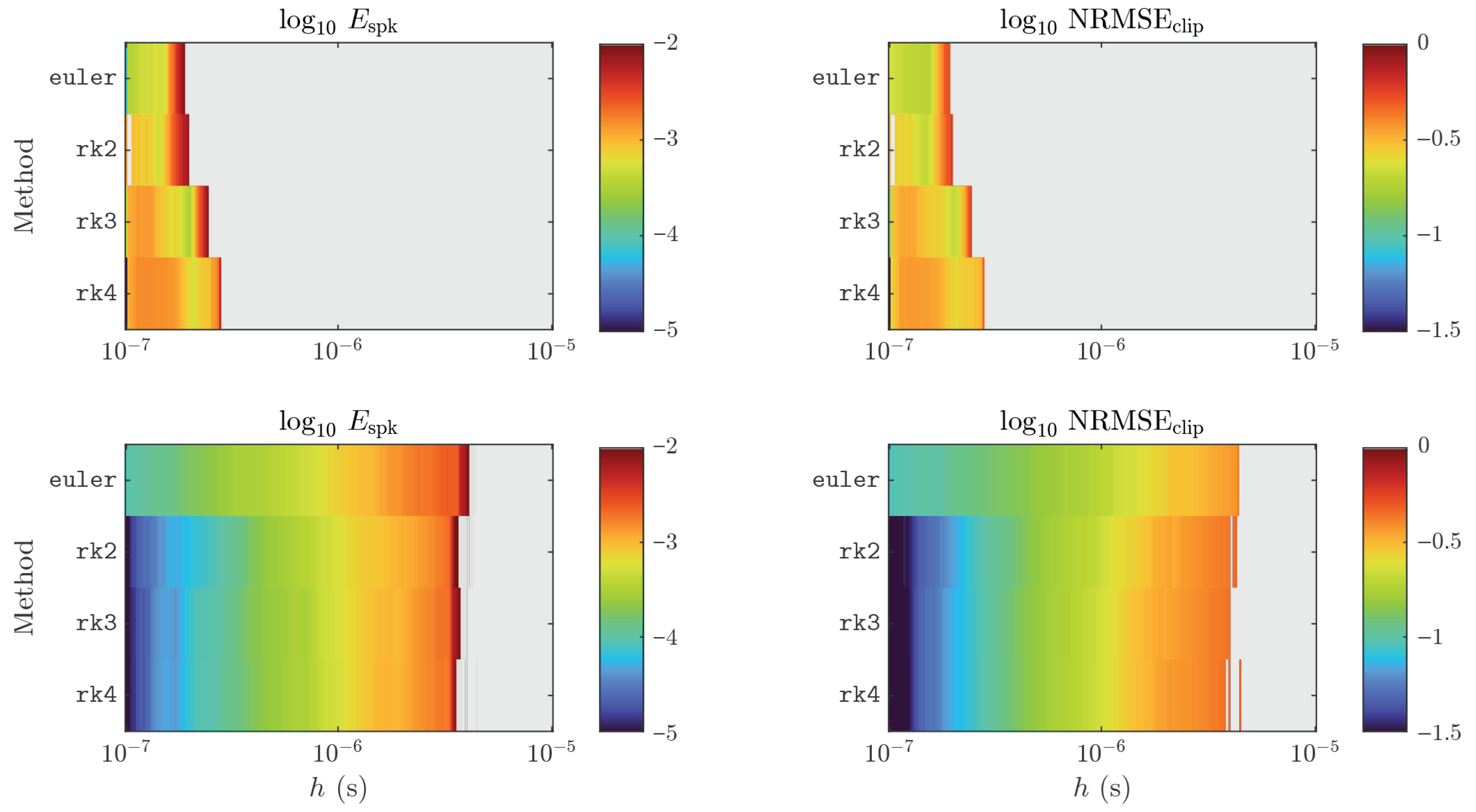
Thus, replacing the TS–TD equations with a parameter-matched Izhikevich surrogate reduces the per-step arithmetic cost by approximately an order of magnitude. Moreover, in Appendix C, we show that in the same simulated time scale, the TS-TD neuron requires a high-order integration method, such as Runge–Kutta fourth order, while the Izhikevich model may be simulated with the same accuracy using a lightweight Euler method and 10 times higher integration step. The overall computational profit of using the Izhikevich surrogate may be estimated as decreasing the simulation time by 2–3 orders of magnitude.

The presented approach establishes a practical bridge between hardware-validated single-neuron dynamics and large-scale network simulation: the Izhikevich model accurately reproduce the spike-train behavior of the TS-TD neuron (as will be further shown in Section 4.3), remaining computationally affordable at the scale of entire network simulation using CPU/GPU.

3. Reservoir Architecture

3.1. Reservoir Types

In reservoir computing, the reservoir is a hidden recurrent layer with a randomly initialized, sparse, and fixed connectivity structure. Its function is to nonlinearly project the input sequence into a high-dimensional state space, where complex temporal dependencies become linearly separable for a simple readout layer. A reservoir possesses two key properties: it consists of individual nonlinear units and has the capacity to store information. The nonlinearity manifests in each unit’s response to an input signal, enabling the solution of complex problems. Reservoirs process data by interconnecting units in recurrent loops, where past input influences subsequent output. This ability to adapt responses based on prior states allows one to train computers to perform specialized tasks.

Many types of reservoir computers have been developed, and the most often used types of them are summarized in

Table 3. Main types of reservoir computing architectures.

Type	Neurons Used	Description	References
Context Reverberation Network	2nd gen	An early implementation of reservoir computing.	[36,37]
Echo State Network (ESN)	2nd gen	A sparsely connected recurrent network with fixed randomly assigned connections	[38,39]
Liquid State Machine (LSM)	3rd gen	A type of reservoir computing that uses a spiking neural network.	[40,41]
Adaptive Reservoir	2nd or 3rd gen	An approach of enhancing the reservoir efficiency through selecting the most suitable one by using an algorithm or a reservoir cluster.	[42,43]

. Note that in the table, an artificial neuron serves as a basic element of a reservoir, though it is not principally limited to use other nonlinear systems, e.g., chaotic flows [35].

Given the context of subsequent transfer of the reservoir implementation from software to hardware, the LSM architecture was chosen. The reason is that ESN is designed for second-generation (non-spiking) neurons, while reservoir adaptation requires either evaluating multiple reservoirs or creating a single, very large one. This would introduce additional complexities in the development of a neuromorphic architecture, which may not be justified relative to the potential performance gains of the reservoir computer by using TS-TD neurons.

3.2. Output Layer

The output layer is responsible for providing the link between the complex dynamics of the reservoir and the task to be solved. Unlike the reservoir, it is trainable, converting the high-dimensional spiking activity into useful output signals (classes, predictions, control commands) [44]. The detailed description of types with references is given in

Table 4. Output layer types.

Type	Description	References
Linear Output Layer	A layer that performs reservoir state transformation via matrix multiplication. The resulting value is used by a trained linear regression model.	[45,46]
Support Vector Machine	Maps the high-dimensional reservoir states into a higher space to find an optimal hyperplane for classification or regression.	[47]
Random Forest	An ensemble method that builds multiple decision trees on reservoir states.	[48]
Perceptron	A perceptron as output layer is used to add nonlinearity to reservoir state transformation. It is trained via backpropagation.	[49,50]
Spiking Output Layer	The type of layer capable of taking spikes from reservoir unchanged, but requires special training algorithms.	[51,52]
Recurrent Output Layer	Recurrent layer adds memory for accounting the history of reservoir activity. Used for data with long-term dependencies.	[53,54]

.

There are several ways to organize the output layer, with the choice depending on the specific task being addressed. In the further study, we explore several types of output layers to find the best choice for a particular dataset under classification.

3.3. LSM Reservoir with Spatially Dependent Random Topology

The recent work by Zhang et al. [28] proposes an approach to form an LSM as a network of neurons organized into a pseudo-spatial three-dimensional structure, where connectivity follows a rule dependent on the probability of a synaptic connection based on the Euclidean distance between neurons. This reservoir architecture maintains a biologically plausible ratio of excitatory to inhibitory neurons [5]. In the current work, this spatially dependent random topology algorithm for LSM is used. Its core concept lies in making the probability of forming a connection between neurons dependent on their coordinates in three-dimensional space. After the topology is formed, a fixed weight is assigned to each connection based on the types of interacting neurons, whether excitatory or inhibitory.

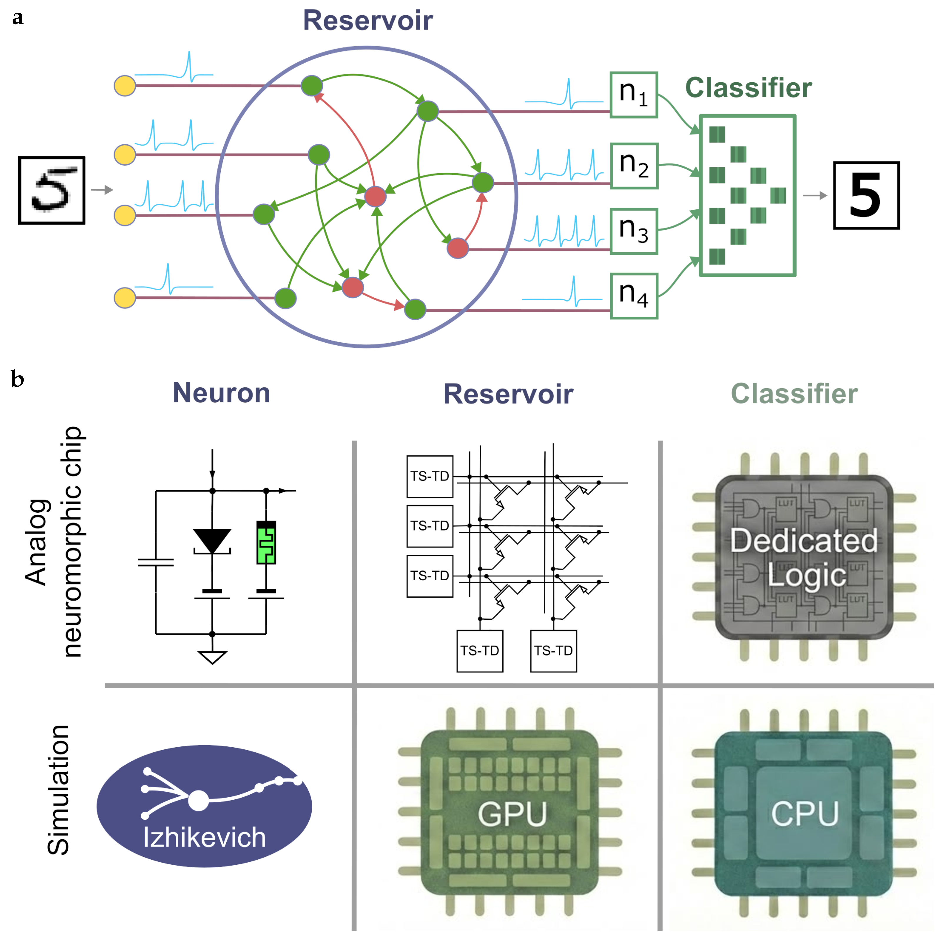
The model comprises a three-layer spiking architecture with the input layer of 784 neurons, a recurrent reservoir of LSM type of 7840 neurons, and an output layer connected to the number of selected neurons, as presented in Figure 2a.

Each neuron in the input layer corresponds to one image pixel. Pixel intensities $I_{\mathrm{pixel}}\in [0,255]$ are mapped to constant external currents. Defining

$$p={\displaystyle \frac{I_{\mathrm{pixel}}}{255}},$$

the injected current is computed as

$$I_{\mathrm{ext}}=70+50p^{1.5},$$

resulting in currents within $[70\dots 120]$ (model units), which correspond to $[4\dots 40]$ spikes in a 1 ms time window. The input remains static during the simulation of a single image; therefore, temporal dynamics emerge exclusively from recurrent reservoir interactions. All neurons (input and reservoir) follow the Izhikevich model described in (4). The same intrinsic dynamics are used for all neurons.

Reservoir neurons are arranged in a three-dimensional lattice of size

$$14\times 16\times 35,$$

with 6237 excitatory (80%) and 1603 inhibitory (20%) neurons [5].

Recurrent connectivity is distance-dependent. The probability of a synaptic connection from neuron i to neuron j is

$$P_{ij}=C_{\mathrm{type}(i,j)}exp\left(-{\left({\displaystyle \frac{d_{ij}}{\lambda }}\right)}^2\right),$$

where $d_{ij}$ denotes the Euclidean lattice distance, $\lambda =3.0$, and connections are limited to a radius of $3\lambda$. The type-dependent coefficients are

$$C=\left[\begin{array}{cc}0.4& 0.4\\ 0.5& 0.0\end{array}\right],$$

corresponding to (E→E, E→I; I→E, I→I). Inhibitory-to-inhibitory connections and autapses are disallowed; reciprocal connections are preserved.

The resulting reservoir contains 351,074 recurrent synapses. The mean indegree and outdegree are both 44.78 (standard deviation $\approx 13.8$), indicating a moderately sparse but homogeneous connectivity regime across the reservoir. Excitatory neurons exhibit a higher mean indegree (47.08) than inhibitory neurons (35.83), which follows from the absence of inhibitory-to-inhibitory projections and the imposed E/I ratio (80/20). Consequently, excitatory neurons integrate a broader set of inputs, while inhibitory neurons act predominantly as regulatory elements within the network. The normalization of incoming weights ensures that the effective synaptic drive remains bounded and prevents structural over-excitation.

Weights are sampled independently from a Gamma distribution with shape parameter $k=2.0$ and mean equal to a type-specific base value:

$$W_{\mathrm{base}}=\left[\begin{array}{cc}0.8& 0.6\\ -0.8& 0\end{array}\right].$$

The sign of each weight is fixed by its connection type, ensuring strictly positive excitatory and strictly negative inhibitory synapses. All incoming weights of each neuron are normalized by its indegree to maintain bounded excitation and stable network activity.

Synaptic transmission is implemented via a threshold-based transduction mechanism. The continuous presynaptic membrane potential is not directly injected into the postsynaptic neuron. Instead, it is converted into a discrete synaptic output level:

$$V_{\mathrm{out}}=\left\{\begin{array}{cc}{V}_{\mathrm{syn}},\hfill & v_{\mathrm{pre}}>-40,\hfill \\ V_{\mathrm{rest}},\hfill & v_{\mathrm{pre}}\le -40.\hfill \end{array}\right.$$

Thus, when the presynaptic neuron exceeds the activation threshold ($-40$), the synapse switches to a high-output state; otherwise, it remains at a controlled baseline level.

Maintaining a finite baseline $V_{\mathrm{rest}}$ keeps postsynaptic neurons within a subthreshold oscillatory regime, preventing full relaxation to the resting equilibrium. This biasing reduces the amplitude and duration of external stimulation required to elicit spikes and accelerates convergence toward stable cyclic activity.

The transduction mechanism effectively implements a gated voltage-level coupling: presynaptic activity controls the activation of a predefined synaptic driving level rather than continuously transmitting analog membrane fluctuations. The resulting coupling can be interpreted as gated level-based interaction: presynaptic threshold crossing activates a predefined synaptic driving level, while subthreshold fluctuations do not continuously propagate. This bounds the magnitude of synaptic drive and decouples synaptic activation from detailed presynaptic waveform shape, yielding well-controlled recurrent excitation in the reservoir.

For input-to-reservoir connections:

$$V_{\mathrm{syn}}=120,V_{\mathrm{rest}}=30,\alpha =1.0.$$

For reservoir-to-reservoir connections:

$$V_{\mathrm{syn}}=120,V_{\mathrm{rest}}=40,\alpha =3.0.$$

The synaptic current contribution to the postsynaptic neuron is proportional to

$$I_{\mathrm{syn}}\propto \alpha w(V_{\mathrm{out}}-v_{\mathrm{post}}),$$

where w is the normalized synaptic weight. We emphasize that all reservoir neurons in the simulation follow the Izhikevich model with parameters fitted to the experimentally validated TS-TD neuron. This ensures that the reported classification performance and energy estimates are grounded in the physical behavior of the proposed hardware neuron, while the surrogate model enables simulation of networks at a scale relevant for practical neuromorphic applications.

4. Results

4.1. Experimental Setup

To validate the TS-TD neuron model, we designed and fabricated a hardware prototype using conventional components. The prototype, shown in Figure 1, consists of three main parts: the AND-TS emulator board mimicking the threshold selector behavior; germanium tunnel diode GI401A, providing negative differential resistance; and ceramic capacitor 2.2 nF for the neuron membrane capacitance.

The AND-TS emulator replicates the negative voltage branch of threshold switching with set voltage $V_{\mathrm{on}}=0.119$ V and reset voltage $V_{\mathrm{off}}=0.03$ V, matching the appropriate parameters of the physical AND-TS device [27]. Key design considerations included: (1) bandwidth $\ge 1$ MHz for all active components to ensure proper switching dynamics; (2) low-pass filters for noise immunity in comparator stages; (3) MOSFET-based set-reset flip-flop for hysteresis implementation compatible with $\pm 15$ V comparators; and (4) MOSFET-based conductive channel applicable for positive voltage drop across emulator’s top and bottom electrodes (TE and BE, respectively). The board was fabricated on two-layer FR4 textolite using rapid prototyping technology. Appendix A provides a circuit schematic and additional details.

Testing conditions were as follows. Input current $I_{in}$ was generated via Rigol DG1032Z arbitrary waveform generator with 1 mV accuracy through series resistor $R_{in}=10$ k$\Omega$. Output voltage $V_{out}$ was captured by Rigol DS1104 digital oscilloscope (100 MHz bandwidth). Phase portraits were observed using analog oscilloscope C1-83 for zero-latency visualization. All measurements were performed at room temperature ($25\pm 2$ °C) with a stabilized $\pm 15$ V 40 W power supply of the NI ELVIS III station.

4.2. Experimental Validation of TS-TD Neuron Circuit Dynamics

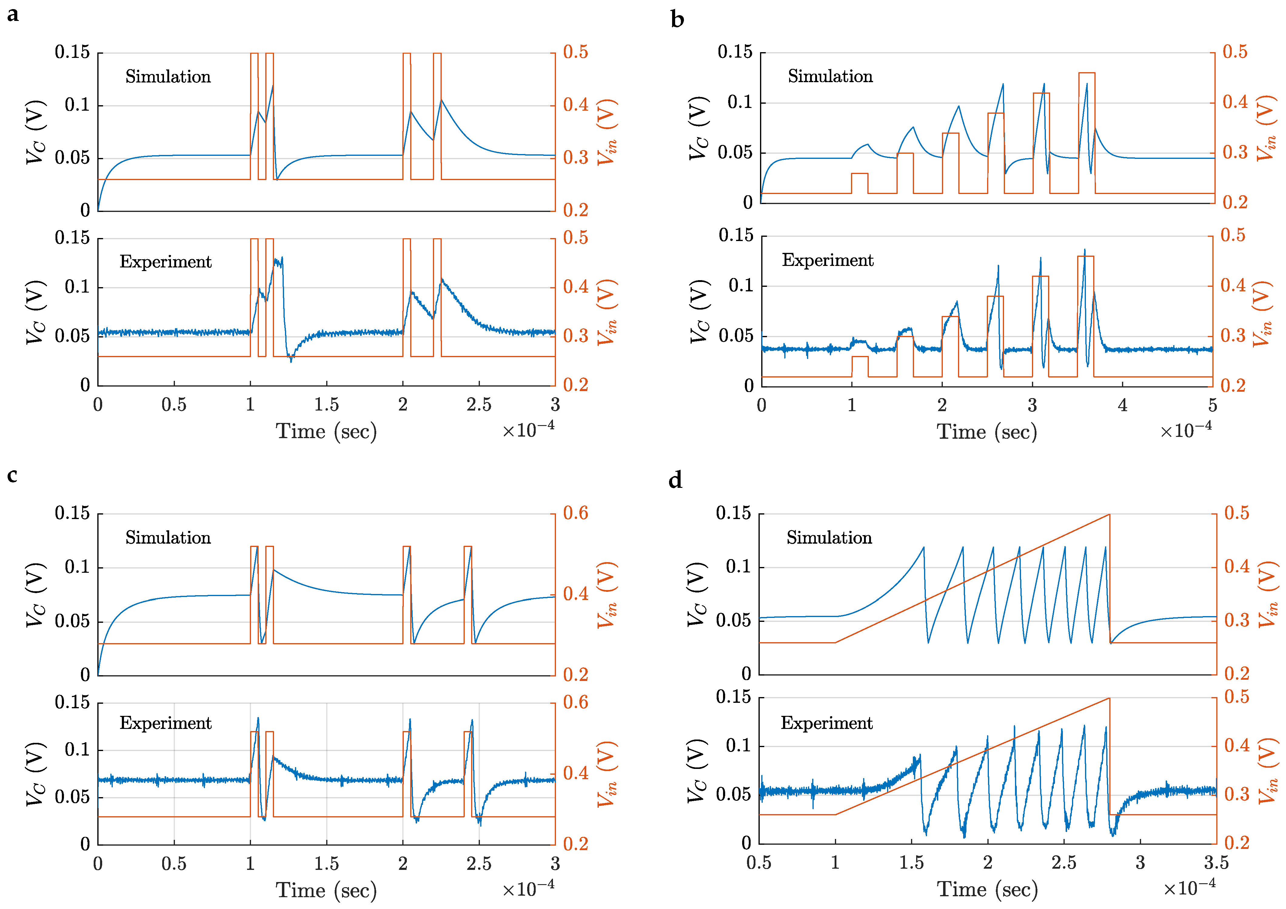
Following exploration of the basic spiking patterns presented by Ostrovskii et al. [25], we performed experiments to validate the similar dynamics. Figure 3 demonstrates experimentally recorded output waveforms $V_{\mathrm{C}}\left(t\right)$ of the TS-TD neuron circuit under an external signal, along with corresponding simulations. The external signal was generated via the arbitrary waveform generator Rigol DG1032 producing voltage $V_{in}\left(t\right)$, converted by series resistor $R_{in}=10\mathrm{k}\Omega$ into current $I_{in}\left(t\right)\approx (V_{in}\left(t\right)-V_C\left(t\right))/R_{\mathrm{in}}$. Stimuli waveforms (shown in Figure 3 as red lines) were beforehand synthesized in MATLAB R2024a, saved as CSV files, and then reproduced by the arbitrary waveform generator with matching of time and amplitude characteristics. Thus, stimuli for both simulation and experiment were kept the same. Recording was performed with a Rigol DS1104 four-channel 100 MHz bandwidth digital oscilloscope.

Figure 3a demonstrates integrator behavior: cumulative subthreshold charging provides spiking only above a critical pulse repetition rate. Figure 3b confirms the all-or-none principle by distinct response to three subthreshold versus three superthreshold input pulses of different amplitudes; specifically, subthreshold stimuli evoke only small output potentials, whereas superthreshold stimuli exceeding the tunnel diode peak current $I_p$ trigger full-amplitude action potentials with AND-TS switching. In Figure 3c, the refractory period $\approx 0.11\mathrm{ms}$ is demonstrated, driven by threshold selector reset kinetics. Figure 3d shows class 1 excitation, which means that the spiking rate increases with the increase of the input voltage. This behavior is different from that presented in [25] due to a lower level of input signal.

Across all tests, experimental data (lower axes) exhibit good agreement with MATLAB R2024a simulations (upper axes). Minor discrepancies are attributed to circuit parasitic parameters, temperature drift, and interferences, providing cycle-to-cycle instabilities. These results validate the general consistency between the TS-TD neuron model and real circuit behavior.

4.3. Consistency Between Izhikevich and TS–TD Neuron Models

To enable efficient large-scale simulations, we identify parameters ${\mathit{\theta }}^{★}$ of an Izhikevich surrogate such that its spike-train statistics match those of the TS–TD neuron under the same stimulus. The identification is posed as

$${\mathit{\theta }}^{★}=arg\underset{\mathit{\theta }}{min}J\left(\mathit{\theta }\right),$$

where J penalizes mismatches in (i) steady-state ISI, (ii) early transient timing, (iii) spike-frequency adaptation, and (iv) total spike count (Appendix B). Importantly, the fit targets spiking behavior (ISI structure and adaptation) rather than pointwise waveform agreement.

The resulting parameter set is

$${\mathit{\theta }}^{★}=(k_I,a,d,\tau ,b,c)=(3.694\times {10}^6,0.1726,20.2734,84640,-0.7844,-61.4219),$$

yielding a low feature-mismatch objective value $J\left({\mathit{\theta }}^{★}\right)\approx 1.56\times {10}^{-5}$.

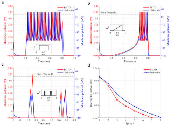
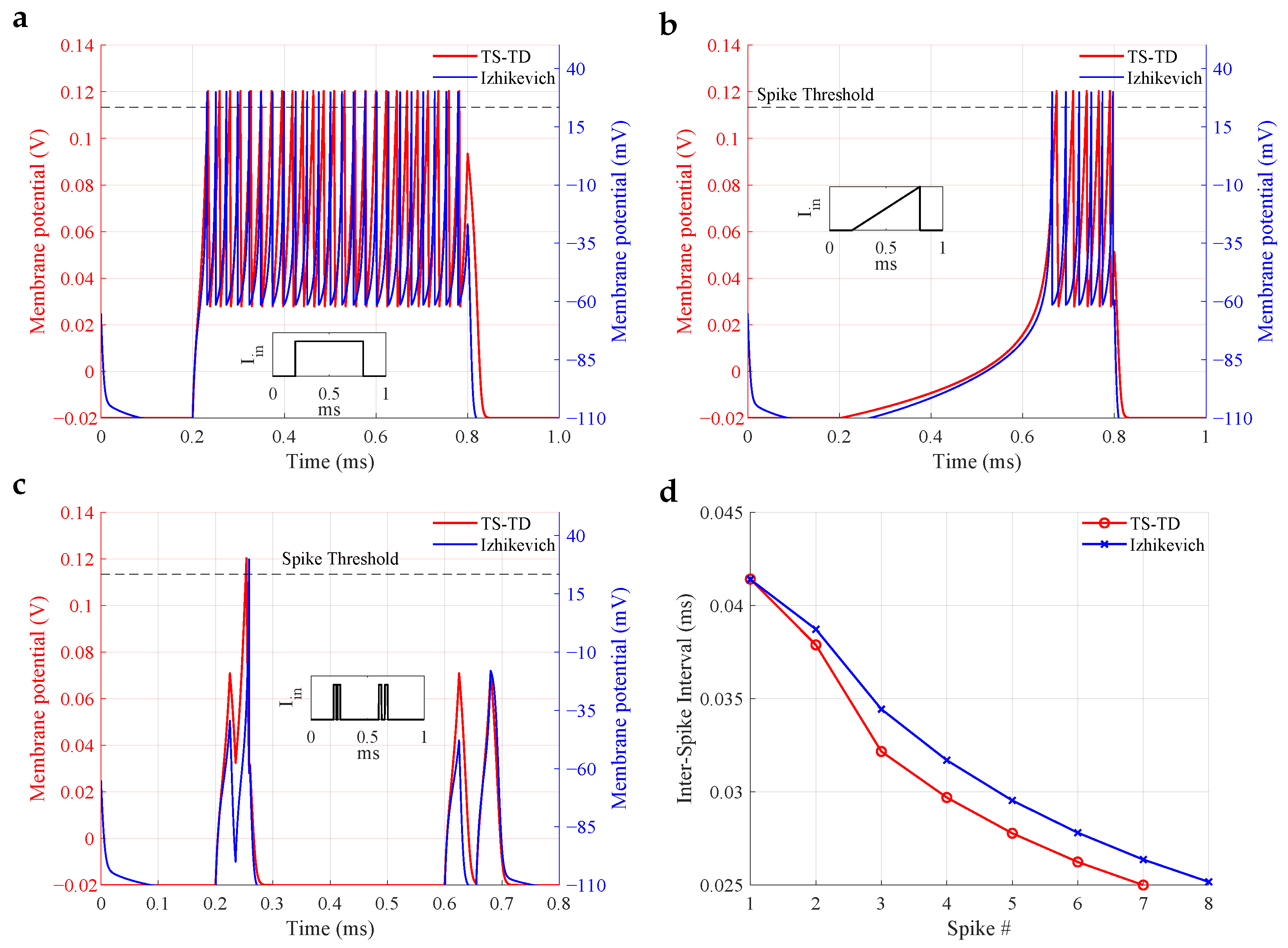
Figure 4 compares representative regimes reproduced by the surrogate: regular tonic spiking, class 1 excitability, integrator-like behavior, and spike-frequency adaptation.

A practical limitation of the TS–TD model is its stricter time-step requirement: stable and spike-faithful integration typically requires $h\lesssim {10}^{-6}\mathrm{s}$, whereas the Izhikevich model remains spike-consistent for $h\sim {10}^{-5}$–${10}^{-4}\mathrm{s}$ (Appendix C). Together with its lower per-step computational cost, this yields an overall speedup, approaching three orders of magnitude in large-scale simulations.

4.4. Reservoir Benchmarking

The computational experiment was conducted on a machine with the specifications presented in

Table 5. Computational environment specifications.

Component	Specification
Hardware
CPU	AMD Ryzen™ 7 9800X3D @ 4.7 GHz (8 cores)
GPU	NVIDIA® GeForce RTX™ 5070 Ti (16 GB VRAM)
RAM	64 GB DDR5 @ 6400 MHz
Software
MATLAB	R2024a
Python	3.13
C++ compiler	MSVC 19.44.35222
CUDA toolkit	13.1 (NVCC 13.1.115)

. The reservoir was stimulated with 30,000 images from the MNIST and Fashion-MNIST datasets. For each stimulus, neuronal activity was summarized by the total number of spikes generated during the presentation interval, forming a high-dimensional feature vector for every image.

Given that each image is represented by a high-dimensional spike-count vector, the resulting feature space is characterized by strong redundancy and inter-neuronal correlations, which are typical for randomly connected reservoirs. In such settings, irrelevant or weakly informative neurons may degrade generalization due to the curse of dimensionality and increased variance of the classifier [55]. Feature selection therefore acts not only as a dimensionality reduction mechanism but also as a regularizer that improves the stability and interpretability of the readout layer [56,57].

In particular, sparsity-inducing methods such as L1-regularized models promote compact subsets of neurons with non-zero contributions to class discrimination [58], while ensemble-based approaches (e.g., random forests) can capture nonlinear feature interactions and provide robust importance estimates in the presence of correlated inputs [59,60]. Such mechanisms are especially relevant for spike-based reservoirs, where multiple neurons may encode partially overlapping dynamical responses to the same stimulus.

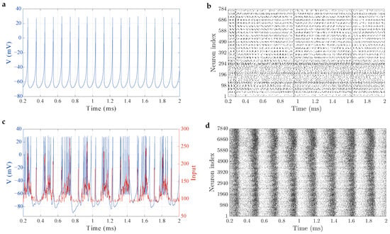
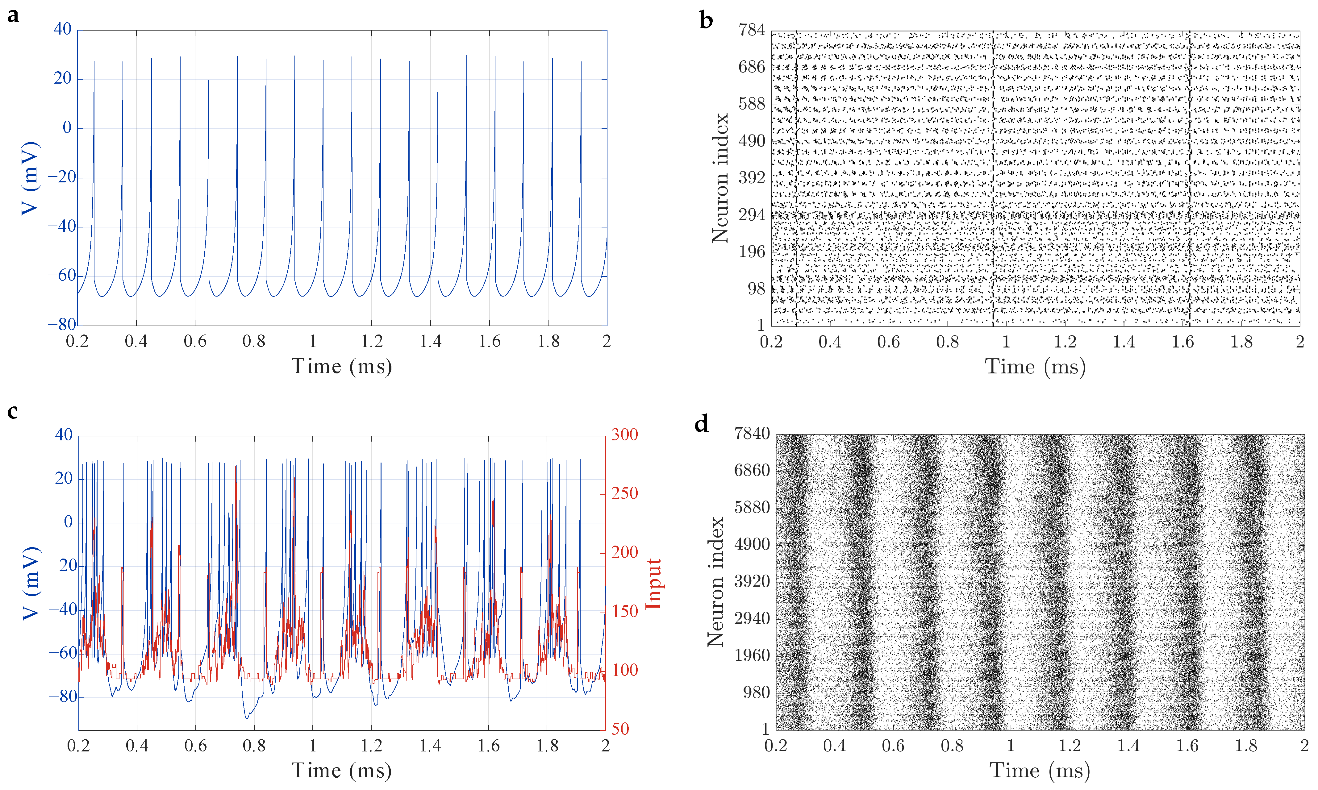
To evaluate the discriminative capability of the reservoir, a systematic study of feature selection, dimensionality reduction, and classifier performance was performed. Five feature selection strategies were considered: ANOVA F-score [56], ${\chi }^2$-criterion [61], absolute correlation with class labels [62], feature importance estimated by a random forest [59], and sparsity-driven ranking based on L1-regularized logistic regression coefficients [63]. For each method, features were ranked in descending order of significance. Spike raster plots evoked by a single T-shirt/top sample from the Fashion-MNIST dataset are given in Figure 5.

From these rankings, subsets of the top-k features were formed with $k\in 100,200,\dots ,1000$. Each subset was used as input to a range of classifiers, including linear support vector machine (SVM), support vector machine with radial basis function (RBF) kernel, k-nearest neighbors, random forest, ridge classifier, logistic regression, and multilayer perceptrons with 3 and 5 hidden layers (with and without dropout regularization). For every combination of feature selector, number of selected features, and classifier, models were trained and evaluated using an $80\%$/$20\%$ train–test split with stratification by class. This resulted in a large-scale sweep across the joint space of feature selection methods, dimensionality levels, and classifier types, allowing identification of the most effective configurations for each dataset.

After this stage, the best-performing classifiers, RBF SVM and the multilayer perceptron, were further fine-tuned using Bayesian hyperparameter optimization to obtain the final reported results and confusion matrices.

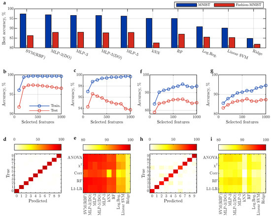
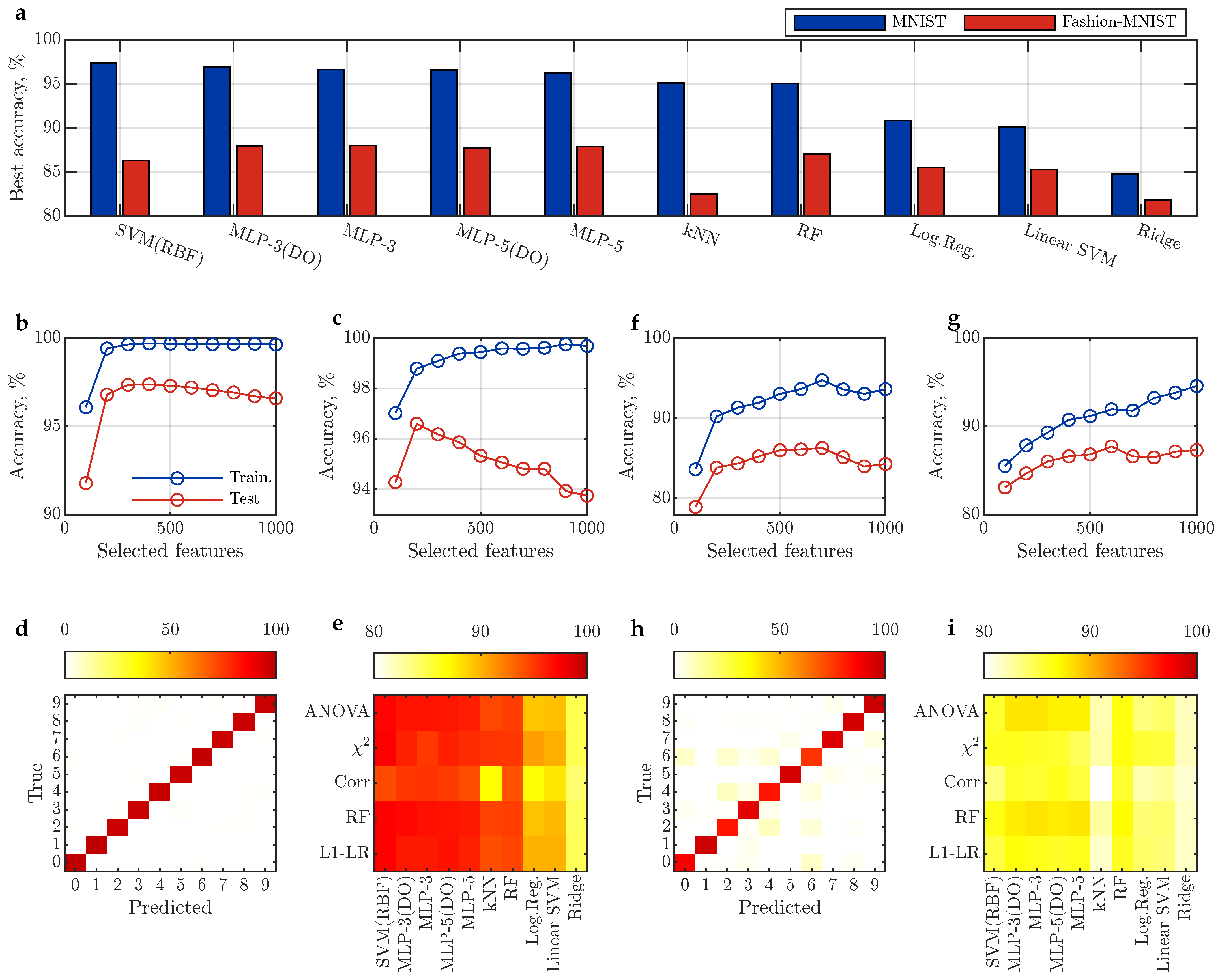
Figure 6 presents plots of the reservoir’s classification accuracy versus the number of neurons used. For the MNIST handwritten digits dataset, the best accuracy was 97.05% for the five-layer perceptron using data from 200 neurons, and 97.9% for the SVM-RBF using data from 400 neurons. A confusion matrix for the latter is shown in Figure 6d. For the Fashion-MNIST clothes images dataset, the best accuracy was 85.67% for the SVM-RBF using data from 700 neurons, and 89.55% for the five-layer perceptron using data from 600 neurons. A confusion matrix for the latter is shown in Figure 6h.

We acknowledge that MNIST and Fashion-MNIST, while widely adopted for initial validation of neuromorphic classifiers, represent relatively simple visual recognition tasks. Their use in this work follows the established practice in reservoir computing literature [40,41] to enable direct comparison with prior LSM implementations. The TS-TD-LSM demonstrates competitive accuracy while offering substantial improvements in estimated energy efficiency and throughput as is shown in Section 4.5. However, we note that cross-platform comparisons should be interpreted with caution due to differences in simulation regarding hardware implementation, output layer complexity, and measurement methodologies. Future work will include evaluation on more complex, event-based datasets such as N-MNIST [64] to further assess the scalability of the proposed approach.

4.5. Neuromorphic Chip Energy and Throughput Estimation

Along with classification accuracy, the important parameters of the neuromorphic chips that drive their development are power consumption and throughput. The total energy consumed to process a single input frame is determined by the cumulative energy of all spikes generated throughout the network during the temporal integration window:

$$E_{\mathrm{frame}}=E_{\mathrm{spike}}·N_{\mathrm{spikes}}\approx E_{\mathrm{spike}}·N_{\mathrm{neurons}}·\overline{r},$$

(5)

where $E_{\mathrm{frame}}$ is expressed in joules per frame (J/frame), $N_{\mathrm{neurons}}$ is a total number of neurons in LSM, and $\overline{r}$ (spikes/neuron/frame) is a mean firing rate for a single neuron. The inference rate per frame is constrained by the temporal integration window for processing:

$$f_{\mathrm{frame}}={\displaystyle \frac{1}{T_{\mathrm{sim}}}}$$

(6)

where $f_{\mathrm{frame}}$ denotes the frame rate in frames per second, and $T_{\mathrm{sim}}$ represents the simulation duration per frame in seconds. For a particular TS-TD-LSM,

Table 6. Parameters for energy and throughput calculations of TS-TD-LSM.

Parameter	Symbol	Value
Energy per spike [25]	$E_{\mathrm{spike}}$	$1.5·{10}^{-10}$ J
Simulation time per frame	$T_{\mathrm{sim}}$	$2·{10}^{-3}$ s
Mean spikes per frame	$N_{\mathrm{spikes}}$	20.5
Number of neurons	$N_{\mathrm{neurons}}$	7840

summarizes the key parameters for required estimation. Substituting the values from Table 6 into (5) and (6) yields:

$$\begin{array}{cc}\hfill E_{\mathrm{frame}}& \approx 1.5·{10}^{-10}\times 7840\times 20.5=2.4·{10}^{-5}\mathrm{J}/\mathrm{frame},\hfill \end{array}$$

(7)

$$\begin{array}{cc}\hfill f_{\mathrm{frame}}& \approx {\displaystyle \frac{1}{2·{10}^{-3}}}=500\mathrm{frames}/\mathrm{s}\hfill \end{array}$$

(8)

The second key value to estimate is the energy consumed by synaptic interaction. A convenient hardware-agnostic proxy for synaptic workload is the number of synaptic operations (SynOps), defined as one delivered presynaptic spike event per outgoing synapse (fanout). For capacitive switching, the dynamic energy per transition is

$$E_{\mathrm{dyn}}\approx \frac{1}{2}{C}_{\mathrm{eff}}{(\Delta V)}^2,\Delta V=V_{\mathrm{syn}}-V_{\mathrm{rest}}.$$

(9)

Typical node capacitance estimates for nanoscale CMOS can be obtained from per-length capacitance: $C_{\mathrm{gate}}\approx 1\mathrm{fF}/\mathsf{\mu }\mathrm{m}$ and $C_{\mathrm{diff}}\approx 0.8\mathrm{fF}/\mathsf{\mu }\mathrm{m}$ [65]. For a transmission-gate-style switch with effective device width on the order of 1 μm, the switched capacitance per synapse is therefore on the order of a few femtofarads; we use

$$C_{\mathrm{eff}}=5\mathrm{fF}$$

(10)

as a representative value (two devices + parasitics).

If the gate remains enabled for duration ${\tau }_{\mathrm{on}}$, an additional leakage/bias term can be included:

$$E_{\mathrm{gate}}\approx \frac{1}{2}{C}_{\mathrm{eff}}{(\Delta V)}^2+\left(I_{\mathrm{leak}}{V}_{\mathrm{DD}}\right){\tau }_{\mathrm{on}}.$$

(11)

For 28 nm-class technologies, $V_{\mathrm{DD}}\approx 0.9$ V is typical [66]. Leakage depends strongly on device flavor and sizing; reported off-currents span from picoampere-scale in long devices [67] up to ∼1 nA/μm for low-power transistors [68].

In our simulator, $\Delta t={10}^{-7}$ s, and we assume that the gate is active for 100 steps per presynaptic event; hence,

$${\tau }_{\mathrm{on}}=100\Delta t={10}^{-5}\mathrm{s}.$$

(12)

For reservoir-to-reservoir synapses, $V_{\mathrm{syn}}=0.119$ V and $V_{\mathrm{rest}}=0.03$ V, so $\Delta V=0.089$ V. Then, the switching term evaluates to

$$E_{\mathrm{dyn}}\approx \frac{1}{2}·5\times {10}^{-15}·{\left(0.089\right)}^2\approx 2.0\times {10}^{-17}\mathrm{J}(\approx 0.020\mathrm{fJ}),$$

(13)

which is typically negligible compared to the on-time leakage term for long ${\tau }_{\mathrm{on}}$. For two illustrative leakage regimes:

$$\begin{array}{cc}\hfill I_{\mathrm{leak}}=10\mathrm{pA}& \Rightarrow E_{\mathrm{leak}}\approx {10}^{-11}·0.9·{10}^{-5}\approx 9\times {10}^{-17}\mathrm{J}(\approx 0.9\mathrm{fJ}),\hfill \end{array}$$

(14)

$$\begin{array}{cc}\hfill I_{\mathrm{leak}}=1\mathrm{nA}& \Rightarrow E_{\mathrm{leak}}\approx {10}^{-9}·0.9·{10}^{-5}\approx 9\times {10}^{-15}\mathrm{J}(\approx 90\mathrm{fJ}).\hfill \end{array}$$

(15)

Thus,

$$E_{\mathrm{gate}}\approx E_{\mathrm{dyn}}+E_{\mathrm{leak}}\approx 0.09–9\mathrm{fJ}\mathrm{per}\mathrm{synaptic}\mathrm{activation},$$

(16)

depending on leakage.

Finally, the recurrent synaptic energy per frame under the gate proxy is

$$E_{\mathrm{syn},\mathrm{frame}}^{\mathrm{gate}}\approx N_{\mathrm{synop},\mathrm{rec}}{E}_{\mathrm{gate}}.$$

(17)

Using $N_{\mathrm{synop},\mathrm{rec}}\approx 7.2\times {10}^6$ synops/frame gives

$$E_{\mathrm{syn},\mathrm{frame}}^{\mathrm{gate}}\approx (6.62\times {10}^{-10})–(6.48\times {10}^{-8})\mathrm{J}/\mathrm{frame}(\mathrm{for}{I}_{\mathrm{leak}}=10\mathrm{pA}–1\mathrm{nA}).$$

(18)

As seen from (18) and (8), synaptic energy is a few orders lower than energy consumed by neurons; thus, it is not considered in the final comparison presented in

Table 7. Comparison of spiking reservoir classifiers of MNIST benchmark.

Neural Classifier	Accuracy, %	Energy Efficiency, J/Frame	Speed, Frames/s
LSM-SOM N(0,1) [28]	90.0	No data	No data
Two-Level Inhibition SNN [69]	94.1	No data	No data
NALSM [70]	97.6	No data	No data
ELSM-7000 [71]	97.8	No data	No data
1024-1024-60 LSM [16]	94.9	$1.3·{10}^{-3}$	89
784-135-26 LSM [72]	96.6	$1.3·{10}^{-1}$	12
Memristive LSM [73]	93.8	$4.0·{10}^{-5}$	250
TS-TD-LSM (this work)	97.9	$2.4·{10}^{-5}$	500

and

Table 8. Comparison of spiking classifiers on Fashion-MNIST benchmark.

Neural Classifier	Accuracy, %	Energy Efficiency, J/Frame	Speed, Frames/s
MAdapter LSM [74]	86.7	No data	No data
Astrocyte-controlled LSM [75]	87.3	No data	No data
NALSM [70]	85.8	No data	No data
ELSM-7000 [71]	88.4	No data	No data
1024-1024-10 FPGA-NHAP [76]	85.1	$4.2·{10}^{-3}$	128
TS-TD-LSM (this work)	89.5	$2.4·{10}^{-5}$	500

.

We emphasize that the energy estimates presented in this section are based on CMOS proxy models and device-level estimations from [25]. In a real neuromorphic chip, several factors may cause deviations from these estimates: (1) process variation in nanoscale transistors affecting leakage currents and switching thresholds; (2) temperature-dependent behavior of tunnel diodes and threshold selectors; (3) parasitic capacitances and resistances in interconnects; and (4) overhead from peripheral circuitry (biasing, routing, I/O). Studies comparing estimated vs. measured energy in fabricated neuromorphic chips report typical deviations of 20–50% [14,73]. Despite these uncertainties, the order-of-magnitude advantage of the TS-TD-LSM in energy efficiency (Table 7) still suggests robust potential for hardware implementation.

4.6. Comparison with Recent Reservoir Architectures

The developed reservoir was compared with similar models implementing liquid state machines (LSMs) based on key metrics: accuracy, energy efficiency, and speed, as shown in Table 7. Recent advances in neural cell architectures [77] also demonstrate efficient spiking networks, though our TS-TD approach offers specific advantages in analog hardware implementation. In terms of accuracy, the TS-TD-neuron-based reservoir significantly outperforms the LSM-SOM N(0,1) model [28], which served as its basis.

The 1024-1024-60 LSM [16] and 784-135-26 LSM [72] reservoirs were implemented in FPGA hardware; therefore, additional metrics such as inference energy efficiency and inference speed were calculated for them. A similar comparison was made for the Fashion-MNIST dataset (see Table 8).

The key limitation of this comparison is that the accuracy, energy efficiency, and throughput were obtained in simulation, not in a real neuromorphic chip. Based on studies that compare the hardware reservoir model and the real chip, e.g., [73], a slight decrease in all characteristics can be expected, which in our case still keeps the developed design attractive and promising. Another limitation is that the output layer is also not accounted for in the estimation of energy consumption and throughput, but it has much simpler structure and number of elements than the reservoir, and for initial evaluation, it can be omitted. Additionally, systematic noise analysis was not included in this study. While the experimental results in Section 4.1 demonstrate stability despite circuit parasitics and interferences, a detailed evaluation of noise robustness in the SNN model is planned for future work.

5. Discussion

The experiments presented in this work demonstrate the feasibility of the TS-TD neuron for both operations as a physically implemented device, and as a basic unit of efficient large-scale neuromorphic network. However, several considerations are important for transitioning from the discrete-component prototype to an integrated neuromorphic chip.

The first notable issue is the power estimation. The energy consumption of 150 pJ per spike [25] results in $2.4·{10}^{-5}$ J/frame, and power consumption of the chip at the proposed frame rate is, thus, $P=2.4·{10}^{-5}·500=0.012$ W, which is an ultimately low value for embedded applications, indicating that the proposed chip may operate without any dedicated cooling. For comparison, the NVIDIA Jetson Nano consumes 5–25 W at video stream processing tasks. However, the energy efficiency of the large-scale reservoir may be further enhanced by power gating for inactive neurons, and by other techniques.

Another important issue is the potential for miniaturization. Our prototype occupies approximately 50 cm² on a PCB. For chip-level implementation, the AND-TS emulator will be replaced with an actual Ag nanodots threshold selector device, fabricated in a compact 5 × 5 µm footprint [27]. The tunnel diode can be fabricated as small as to occupy a square of 0.1 µ${\mathrm{m}}^2$ [78]. The membrane capacitor is the most space-demanding part. Using TaTiO high-k dielectric with capacitance of 23 fF/µ${\mathrm{m}}^2$ [79], a 2.2 nF sample requires about ${10}^5$ µ${\mathrm{m}}^2$, resulting in ≈10,000 neurons on a square of large server-grade chip. This is still sufficient for implementing the proposed reservoir computer. With that, using a smaller membrane capacitor, much higher integration density and operation rate are possible, which is a subject for the further study.

The verification part of the current research focuses on hardware neuron dynamics, while synaptic connections were simulated on the functional rather than physical level. For the complete hardware implementation, semiconductor synapses with controllable weights need to be introduced. Recent advances in memristive crossbar arrays provide a promising pathway for dense, energy-efficient synaptic grids [73]. The key challenge with memristors is their intercycle variability. However, reservoir computing does not require precise weight tuning, as its performance depends primarily on spectral radius rather than exact weight values [80]. This confirms robustness against moderate weights variations, as well as persistent noise in the reservoir, which, moreover, may be specifically considered at the training stage [81]. In total, the memristive synaptic grid is a promising subject for further research and development, along with systematic study of its variable impact on the network performance.

6. Conclusions

This work aims to design a reservoir computer based on a novel hardware model of a spiking neuron, constructed from three elements (threshold selector, tunnel diode, and capacitor), called a TS-TD neuron for short. This model implements a simplified version of Hodgkin–Huxley neuron by means of analog electronics and can exhibit a variety of behavior modes, e.g., it can work either as an integrator or a resonator, similar to the computationally efficient Izhikevich model feasible for digital computers. The analog nature of the TS-TD neuron allows a significant reduction of power and increases the speed of large-scale neural networks.

To estimate the performance of a TS-TD neuron-based large-scale network, we developed a software implementation of a liquid state machine (LSM)-type reservoir computer, utilizing 7840 neurons and 351,074 synapses between them, and executed on a GPU using the CUDA library. For the output layer, we compared several classifiers, among which support vector machine with radial basis function kernel and five-layer perceptron with dropout gave the best results.

Solving the task of image recognition from the MNIST and Fashion-MNIST datasets yielded a classification accuracy of 97.9% and 89.5%, respectively, which is a good result for known LSM implementations. With that, the estimated frame rate of the reservoir, if it was implemented on an analog neuromorphic chip, is compared with known implementations in FPGA, and surpasses them by two orders of magnitude in energy efficiency, demonstrating consumption similar to state-of-the-art memristive chips.

Key limitations of the study include: (1) results obtained in simulation rather than on a physical neuromorphic chip; (2) output layer energy consumption not included in estimates; and (3) hardware synapses needs to be proposed in detail. Future work will aim to address these issues, as well as consider experiments on adaptation, including astrocyte control, and further clarification of neuromorphic chip design.

References

- Tavanaei, A.; Ghodrati, M.; Kheradpisheh, S.R.; Masquelier, T.; Maida, A. Deep learning in spiking neural networks. Neural Netw. 2019, 111, 47–63. [Google Scholar] [CrossRef] [Scilit]
- Philipp, G.; Song, D.; Carbonell, J.G. The exploding gradient problem demystified-definition, prevalence, impact, origin, tradeoffs, and solutions. arXiv 2017, arXiv:1712.05577. [Google Scholar]
- Davidson, S.; Furber, S.B. Comparison of artificial and spiking neural networks on digital hardware. Front. Neurosci. 2021, 15, 651141. [Google Scholar] [CrossRef] [Scilit] [PubMed]
- Przyczyna, D.; Pecqueur, S.; Vuillaume, D.; Szaciłowski, K. Reservoir computing for sensing: An experimental approach. arXiv 2020, arXiv:2001.04342. [Google Scholar] [CrossRef] [Scilit]
- Lukoševičius, M.; Jaeger, H. Reservoir computing approaches to recurrent neural network training. Comput. Sci. Rev. 2009, 3, 127–149. [Google Scholar] [CrossRef] [Scilit]
- Morando, S.; Pera, M.; Steiner, N.Y.; Jemei, S.; Hissel, D.; Larger, L. Reservoir Computing optimisation for PEM fuel cell fault diagnostic. In Proceedings of the 2017 IEEE Vehicle Power and Propulsion Conference (VPPC); IEEE: New York, NY, USA, 2017; pp. 1–7. [Google Scholar]
- Zhang, S.; Duan, X.; Li, C.; Liang, M. Pre-classified reservoir computing for the fault diagnosis of 3D printers. Mech. Syst. Signal Process. 2021, 146, 106961. [Google Scholar] [CrossRef] [Scilit]
- McCulloch, W.S.; Pitts, W. A logical calculus of the ideas immanent in nervous activity. Bull. Math. Biophys. 1943, 5, 115–133. [Google Scholar] [CrossRef] [Scilit]
- Cybenko, G. Approximation by superpositions of a sigmoidal function. Math. Control Signals Syst. 1989, 2, 303–314. [Google Scholar] [CrossRef] [Scilit]
- Gerstner, W.; Kistler, W.M. Spiking Neuron Models: Single Neurons, Populations, Plasticity; Cambridge University Press: Cambridge, UK, 2002. [Google Scholar]
- Tschand, A.; Rajan, A.T.R.; Idgunji, S.; Ghosh, A.; Holleman, J.; Kiraly, C.; Ambalkar, P.; Borkar, R.; Chukka, R.; Cockrell, T.; et al. MLPerf Power: Benchmarking the Energy Efficiency of Machine Learning Systems from μWatts to MWatts for Sustainable AI. In Proceedings of the 2025 IEEE International Symposium on High Performance Computer Architecture (HPCA); IEEE: New York, NY, USA, 2025; pp. 1201–1216. [Google Scholar]
- Li, D.; Chen, X.; Becchi, M.; Zong, Z. Evaluating the energy efficiency of deep convolutional neural networks on CPUs and GPUs. In Proceedings of the 2016 IEEE International Conferences on Big Data and Cloud Computing (BDCloud), Social Computing and Networking (SocialCom), Sustainable Computing and Communications (SustainCom) (BDCloud-SocialCom-SustainCom); IEEE: New York, NY, USA, 2016; pp. 477–484. [Google Scholar]
- Ye, J.; Wang, W.; Shi, C.; Cui, X.; Qu, W.; Lin, P.; Yu, X.; Cheng, R.; Wu, H.; Chen, B. An overhead-reduced, efficient, fully analog neural-network computing hardware. Sci. Adv. 2025, 11, eadv7555. [Google Scholar] [CrossRef] [Scilit]
- Davies, M.; Wild, A.; Orchard, G.; Sandamirskaya, Y.; Guerra, G.A.F.; Joshi, P.; Plank, P.; Risbud, S.R. Advancing neuromorphic computing with loihi: A survey of results and outlook. Proc. IEEE 2021, 109, 911–934. [Google Scholar] [CrossRef] [Scilit]
- Cheng, H.P.; Wen, W.; Wu, C.; Li, S.; Li, H.H.; Chen, Y. Understanding the design of IBM neurosynaptic system and its tradeoffs: A user perspective. In Proceedings of the Design, Automation & Test in Europe Conference & Exhibition (DATE); IEEE: New York, NY, USA, 2017; pp. 139–144. [Google Scholar]
- Shi, C.; Fu, X.; Wang, H.; Lin, Y.; Jiang, Y.; Liu, L.; Wu, N.; Tian, M. Ghost reservoir: A memory-efficient low-power and real-time neuromorphic processor of liquid state machine with on-chip learning. IEEE Trans. Circuits Syst. II Express Briefs 2024, 71, 4526–4530. [Google Scholar] [CrossRef] [Scilit]
- Lou, X.; Zan, H.; Wang, Z.; Shi, J.; Zhang, S. Privacy-preserving bidirectional data transmission of smart grid via semi-quantum computation: On mutual identity and message authentication. IEEE Trans. Dependable Secur. Comput. 2025, 22, 5537–5548. [Google Scholar] [CrossRef] [Scilit]
- Stoliar, P.; Schneegans, O.; Rozenberg, M.J. Biologically relevant dynamical behaviors realized in an ultra-compact neuron model. Front. Neurosci. 2020, 14, 421. [Google Scholar] [CrossRef] [Scilit] [PubMed]
- Ranjan, R.; Kwon, M.W.; Park, J.; Kim, H.; Park, B.G. Neuron circuit using a thyristor and inter-neuron connection with synaptic devices. JSTS J. Semicond. Technol. Sci. 2015, 15, 365–373. [Google Scholar] [CrossRef] [Scilit]
- Tagluk, M.E.; Isik, I. Communication in nano devices: Electronic based biophysical model of a neuron. Nano Commun. Netw. 2019, 19, 134–147. [Google Scholar] [CrossRef] [Scilit]
- Isik, I.; Tagluk, M.E. Analysis of the electronic integrate and fire neuron model. Neurocomputing 2022, 488, 261–270. [Google Scholar] [CrossRef] [Scilit]
- Pickett, M.D.; Medeiros-Ribeiro, G.; Williams, R.S. A scalable neuristor built with Mott memristors. Nat. Mater. 2013, 12, 114–117. [Google Scholar] [CrossRef] [Scilit]
- Li, Y.; Tang, J.; Gao, B.; Li, X.; Xi, Y.; Zhang, W.; Qian, H.; Wu, H. Oscillation neuron based on a low-variability threshold switching device for high-performance neuromorphic computing. J. Semicond. 2021, 42, 064101. [Google Scholar] [CrossRef] [Scilit]
- Yuan, R.; Duan, Q.; Tiw, P.J.; Li, G.; Xiao, Z.; Jing, Z.; Yang, K.; Liu, C.; Ge, C.; Huang, R.; et al. A calibratable sensory neuron based on epitaxial VO2 for spike-based neuromorphic multisensory system. Nat. Commun. 2022, 13, 3973. [Google Scholar] [CrossRef] [Scilit]
- Ostrovskii, V.; Karimov, T.; Rybin, V.; Bobrova, Y.; Arlyapov, V.; Butusov, D. Bio-inspired neuron based on threshold selector and tunnel diode capable of excitability modulation. Neurocomputing 2025, 624, 129454. [Google Scholar] [CrossRef] [Scilit]
- Hodgkin, A.L. The local electric changes associated with repetitive action in a non-medullated axon. J. Physiol. 1948, 107, 165–181. [Google Scholar] [CrossRef] [Scilit] [PubMed]
- Hua, Q.; Wu, H.; Gao, B.; Zhao, M.; Li, Y.; Li, X.; Hou, X.; Chang, M.F.; Zhou, P.; Qian, H. A threshold switching selector based on highly ordered Ag nanodots for X-point memory applications. Adv. Sci. 2019, 6, 1900024. [Google Scholar] [CrossRef] [Scilit] [PubMed]
- Zhang, Y.; Mo, L.; He, X.; Meng, X. Unsupervised spiking neural network based on liquid state machine and self-organizing map. Neurocomputing 2025, 620, 129120. [Google Scholar] [CrossRef] [Scilit]
- Izhikevich, E.M. Resonate-and-fire neurons. Neural Netw. 2001, 14, 883–894. [Google Scholar] [CrossRef] [Scilit] [PubMed]
- Wilson, H.R. Spikes, Decisions, and Actions: The Dynamical Foundations of Neuroscience; Oxford University Press: Oxford, UK, 1999. [Google Scholar]
- Nagumo, J.; Arimoto, S.; Yoshizawa, S. An active pulse transmission line simulating nerve axon. Proc. IRE 2007, 50, 2061–2070. [Google Scholar] [CrossRef] [Scilit]
- Izhikevich, E. Which model to use for cortical spiking neurons? IEEE Trans. Neural Netw. 2004, 15, 1063–1070. [Google Scholar] [CrossRef] [Scilit]
- Bolshakov, D.I.; Mishchenko, M.A.; Chindarev, D.V.; Matrosov, V.V. Recursive map neuron model. In Proceedings of the 2024 8th Scientific School Dynamics of Complex Networks and Their Applications (DCNA); IEEE: New York, NY, USA, 2024; pp. 23–26. [Google Scholar]
- Bolshakov, D.I.; Chindarev, D.V.; Matrosov, V.V.; Mishchenko, M.A. Discrete recursive map neuron model. Eur. Phys. J. Spec. Top. 2025, 234, 8583–8592. [Google Scholar] [CrossRef] [Scilit]
- Kesgin, B.U.; Teğin, U. Implementing the analogous neural network using chaotic strange attractors. Commun. Eng. 2024, 3, 99. [Google Scholar] [CrossRef] [Scilit]
- Kirby, K. Context dynamics in neural sequential learning. In Proceedings of the 4th Florida Artificial Intelligence Research Symposium (FLAIRS 1991), Cocoa Beach, FL, USA, 2–5 April 1991; Volume 66, pp. 66–170. [Google Scholar]
- Kirby, K.; Day, N. The neurodynamics of context reverberation learning. In Proceedings of the Twelfth Annual International Conference of the IEEE Engineering in Medicine and Biology Society; IEEE: New York, NY, USA, 1990; pp. 1781–1782. [Google Scholar]
- Gallicchio, C.; Micheli, A. Deep tree echo state networks. In Proceedings of the 2018 International Joint Conference on Neural Networks (IJCNN); IEEE: New York, NY, USA, 2018; pp. 1–8. [Google Scholar]
- Jaeger, H.; Haas, H. Harnessing nonlinearity: Predicting chaotic systems and saving energy in wireless communication. Science 2004, 304, 78–80. [Google Scholar] [CrossRef] [Scilit]
- Maass, W.; Natschläger, T.; Markram, H. Real-time computing without stable states: A new framework for neural computation based on perturbations. Neural Comput. 2002, 14, 2531–2560. [Google Scholar] [CrossRef] [Scilit]
- Schrauwen, B.; D’Haene, M.; Verstraeten, D.; Van Campenhout, J. Compact hardware liquid state machines on FPGA for real-time speech recognition. Neural Netw. 2008, 21, 511–523. [Google Scholar] [CrossRef] [Scilit] [PubMed]
- van der Zant, T.; Bečanović, V.; Ishii, K.; Kobialka, H.U.; Ploeger, P. Finding good echo state networks to control an underwater robot using evolutionary computations. IFAC Proc. Vol. 2004, 37, 215–220. [Google Scholar] [CrossRef] [Scilit]
- Steil, J.J. Online reservoir adaptation by intrinsic plasticity for backpropagation–decorrelation and echo state learning. Neural Netw. 2007, 20, 353–364. [Google Scholar] [CrossRef] [Scilit] [PubMed]
- Zhang, Y.; Li, P.; Jin, Y.; Choe, Y. A digital liquid state machine with biologically inspired learning and its application to speech recognition. IEEE Trans. Neural Netw. Learn. Syst. 2015, 26, 2635–2649. [Google Scholar] [CrossRef] [Scilit]
- Alaíz, C.M.; Dorronsoro, J.R. On the learning of ESN linear readouts. In Proceedings of the Conference of the Spanish Association for Artificial Intelligence; Springer: Berlin/Heidelberg, Germany, 2011; pp. 124–133. [Google Scholar]
- Li, Z.; Tanaka, G. Multi-reservoir echo state networks with sequence resampling for nonlinear time-series prediction. Neurocomputing 2022, 467, 115–129. [Google Scholar] [CrossRef] [Scilit]
- Alalshekmubarak, A.; Smith, L.S. A novel approach combining recurrent neural network and support vector machines for time series classification. In Proceedings of the 2013 9th International Conference on Innovations in Information Technology (IIT); IEEE: New York, NY, USA, 2013. [Google Scholar]
- Lee, E.; Nam, J.Y.; Ko, B. Speed-limit sign recognition using convolutional neural network based on random forest. J. Broadcast Eng. 2015, 20, 938–949. [Google Scholar] [CrossRef] [Scilit]
- Sedki, K.; Yi, Y.C. Advancing Analog Reservoir Computing through Temporal Attention and MLP Integration. In Proceedings of the 2024 25th International Symposium on Quality Electronic Design (ISQED); IEEE: New York, NY, USA, 2024; pp. 1–8. [Google Scholar]
- Köster, F.; Kanno, K.; Ohkubo, J.; Uchida, A. Attention-enhanced reservoir computing. Phys. Rev. Appl. 2024, 22, 014039. [Google Scholar] [CrossRef] [Scilit]
- Paugam-Moisy, H.; Martinez, R.; Bengio, S. Delay learning and polychronization for reservoir computing. Neurocomputing 2008, 71, 1143–1158. [Google Scholar] [CrossRef] [Scilit]
- Gaurav, R.; Stewart, T.C.; Yi, Y. Reservoir based spiking models for univariate Time Series Classification. Front. Comput. Neurosci. 2023, 17, 1148284. [Google Scholar] [CrossRef] [Scilit]
- Holzmann, G.; Hauser, H. Echo state networks with filter neurons and a delay&sum readout. Neural Netw. 2010, 23, 244–256. [Google Scholar]
- Ohkubo, A.; Inubushi, M. Reservoir computing with generalized readout based on generalized synchronization. Sci. Rep. 2024, 14, 30918. [Google Scholar] [CrossRef] [Scilit] [PubMed]
- Bellman, R. Adaptive Control Processes: A Guided Tour; Princeton University Press: Princeton, NJ, USA, 1961. [Google Scholar]
- Guyon, I.; Elisseeff, A. An introduction to variable and feature selection. J. Mach. Learn. Res. 2003, 3, 1157–1182. [Google Scholar]
- Saeys, Y.; Inza, I.; Larrañaga, P. A review of feature selection techniques in bioinformatics. Bioinformatics 2007, 23, 2507–2517. [Google Scholar] [CrossRef] [Scilit] [PubMed]
- Tibshirani, R. Regression shrinkage and selection via the lasso. J. R. Stat. Soc. Ser. B 1996, 58, 267–288. [Google Scholar] [CrossRef] [Scilit]
- Breiman, L. Random forests. Mach. Learn. 2001, 45, 5–32. [Google Scholar] [CrossRef] [Scilit]
- Li, J.; Cheng, K.; Wang, S.; Morstatter, F.; Trevino, R.P.; Tang, J.; Liu, H. Feature selection: A data perspective. ACM Comput. Surv. 2017, 50, 94. [Google Scholar] [CrossRef] [Scilit]
- Forman, G. An extensive empirical study of feature selection metrics for text classification. J. Mach. Learn. Res. 2003, 3, 1289–1305. [Google Scholar]
- Hall, M.A.; Holmes, G. Benchmarking attribute selection techniques for discrete class data mining. IEEE Trans. Knowl. Data Eng. 2003, 15, 1437–1447. [Google Scholar] [CrossRef] [Scilit]
- Friedman, J.H.; Hastie, T.; Tibshirani, R. Regularization paths for generalized linear models via coordinate descent. J. Stat. Softw. 2010, 33, 1–22. [Google Scholar] [CrossRef] [Scilit]
- Orchard, G.; Jayawant, A.; Cohen, G.K.; Thakor, N. Converting static image datasets to spiking neuromorphic datasets using saccades. Front. Neurosci. 2015, 9, 437. [Google Scholar] [CrossRef] [Scilit]
- Harris, D.; Harris, S. Lecture 7: Power. PDF lecture slides, CMOS VLSI Design. 2009. Available online: https://pages.hmc.edu/harris/class/e158/lect7-power.pdf (accessed on 1 April 2026).
- Pipino, A. Design of Analog Circuits in 28 nm CMOS Technology. Ph.D. Thesis, Università degli Studi di Milano-Bicocca, Milan, Italy, 2019. [Google Scholar]
- Moradi, S.; Bhave, S.A.; Manohar, R. Energy-efficient Hybrid CMOS-NEMS LIF Neuron Circuit in 28 nm CMOS. In Proceedings of the IEEE Symposium Series on Computational Intelligence (SSCI); IEEE: New York, NY, USA, 2017. [Google Scholar]
- TSMC Research. Logic Transistor Structure (Publish-Time Page 4). Available online: https://research.tsmc.com/english/research/logic/transistor-structure/publish-time-4.html (accessed on 1 April 2026).
- Hazan, H.; Saunders, D.J.; Sanghavi, D.T.; Siegelmann, H.; Kozma, R. Lattice map spiking neural networks (LM-SNNs) for clustering and classifying image data. Ann. Math. Artif. Intell. 2020, 88, 1237–1260. [Google Scholar] [CrossRef] [Scilit]
- Ivanov, V.; Michmizos, K. Increasing liquid state machine performance with edge-of-chaos dynamics organized by astrocyte-modulated plasticity. Adv. Neural Inf. Process. Syst. 2021, 34, 25703–25719. [Google Scholar]
- Pan, W.; Zhao, F.; Han, B.; Dong, Y.; Zeng, Y. Emergence of brain-inspired small-world spiking neural network through neuroevolution. iScience 2024, 27, 108845. [Google Scholar] [CrossRef] [Scilit] [PubMed]
- Wang, Q.; Jin, Y.; Li, P. General-purpose LSM learning processor architecture and theoretically guided design space exploration. In Proceedings of the 2015 IEEE Biomedical Circuits and Systems Conference (BioCAS); IEEE: New York, NY, USA, 2015; pp. 1–4. [Google Scholar]
- Henderson, A.; Yakopcic, C.; Merkel, C.; Hazan, H.; Harbour, S.; Taha, T.M. Memristor Based Liquid State Machine With Method for In-Situ Training. IEEE Trans. Nanotechnol. 2024, 23, 376–385. [Google Scholar] [CrossRef] [Scilit]
- Biswas, A.; Nambiar, N.S.; Kejriwal, K.; Ganguly, U. Madapter: A multimodal adapter for liquid state machines configures the input layer for the same reservoir to enable vision and speech classification. In Proceedings of the 2023 International Joint Conference on Neural Networks (IJCNN); IEEE: New York, NY, USA, 2023; pp. 1–6. [Google Scholar]
- Gudur, H. Astrocyte-Gated Dual Coupled Liquid State Machines at the Edge of Chaos. Ph.D. Thesis, Rutgers University-School of Graduate Studies, New Brunswick, NJ, USA, 2026. [Google Scholar]
- Liu, Y.; Chen, Y.; Ye, W.; Gui, Y. FPGA-NHAP: A general FPGA-based neuromorphic hardware acceleration platform with high speed and low power. IEEE Trans. Circuits Syst. I Regul. Pap. 2022, 69, 2553–2566. [Google Scholar] [CrossRef] [Scilit]
- Khalil, K.; Kumar, A.; Bayoumi, M. An efficient neural cell architecture for spiking neural networks. IEEE Open J. Comput. Soc. 2025, 6, 599–612. [Google Scholar] [CrossRef] [Scilit]
- Pawlik, D.; Romanczyk, B.; Freeman, E.; Thomas, P.; Barth, M.; Rommel, S.; Cheng, Z.; Li, J.; Park, J.; Hydrick, J.; et al. Sub-micron Esaki tunnel diode fabrication and characterization. In Proceedings of the 2009 International Semiconductor Device Research Symposium; IEEE: New York, NY, USA, 2009; pp. 1–2. [Google Scholar]
- Chiang, K.; Lai, C.; Chin, A.; Wang, T.; Chiu, H.; Chen, J.R.; McAlister, S.; Chi, C. Very high-density (23 fF/μm2) RF MIM capacitors using high-/spl kappa/TaTiO as the dielectric. IEEE Electron Device Lett. 2005, 26, 728–730. [Google Scholar] [CrossRef] [Scilit]
- Strauss, T.; Wustlich, W.; Labahn, R. Design strategies for weight matrices of echo state networks. Neural Comput. 2012, 24, 3246–3276. [Google Scholar] [CrossRef] [Scilit]
- Wikner, A.; Harvey, J.; Girvan, M.; Hunt, B.R.; Pomerance, A.; Antonsen, T.; Ott, E. Stabilizing machine learning prediction of dynamics: Novel noise-inspired regularization tested with reservoir computing. Neural Netw. 2024, 170, 94–110. [Google Scholar] [CrossRef] [Scilit]
Disclaimer/Publisher’s Note: The statements, opinions and data contained in all publications are solely those of the individual author(s) and contributor(s) and not of MDPI and/or the editor(s). MDPI and/or the editor(s) disclaim responsibility for any injury to people or property resulting from any ideas, methods, instructions or products referred to in the content. |
© 2026 by the authors. Licensee MDPI, Basel, Switzerland. This article is an open access article distributed under the terms and conditions of the Creative Commons Attribution (CC BY) license.