A Multi-Feature Transition-Aware Framework for Next POI Recommendation

Abstract

Next Point-of-Interest (POI) recommendation focuses on predicting a user’s subsequent location based on historical check-in data. In practice, however, check-in logs frequently contain uncertain records in which ambiguous spatial, temporal, or behavioral information obscures the underlying mobility regularities, thereby degrading prediction performance. To address this challenge, this study first infers user preferences from historical trajectories and reweights transition importance based on temporal and spatial proximity. It then models transition relationships using three complementary feature dimensions: POI category, spatial area, and routine versus non-routine behavioral patterns. Using transition probability analysis, feature-level dependencies in user mobility are systematically investigated. The findings demonstrate that these transition features contribute unevenly to predictive performance, with area-based transitions yielding the strongest results when used in isolation. Nonetheless, their joint integration consistently achieves the highest accuracy, underscoring the critical role of transition-aware modeling. Across two real-world datasets, the proposed framework consistently achieves state-of-the-art performance in top-ranked accuracy (Recall@1) and ranking quality (NDCG@1), while delivering competitive effectiveness at higher cutoff values ($k=3$ and $k=5$). Notably, on the NYC dataset, MTF-POI achieves the highest Recall@1 (+19.01% over the strongest baseline) with a marginal trade-off at Recall@3, reflecting the framework’s design emphasis on precise next-step prediction.

1. Introduction

The widespread adoption of smartphones and social check-in services has enabled the large-scale collection of user trajectory data through location-based social networking (LBSN) platforms such as Foursquare, Facebook Places, and Google Maps. These data provide rich information about human mobility patterns and support the development of personalized location recommendation systems. Conventional point-of-interest (POI) recommendation methods predominantly model static user–location interactions, typically neglecting the sequential and temporal characteristics inherent in human movement [1,2]. With the increasing availability of large-scale spatiotemporal datasets, research attention has progressively shifted toward the next POI recommendation [3,4,5], which aims to predict the next destination of a user based on current or recent locations. This prediction task is intrinsically challenging, as effective models must jointly capture user-specific preferences, spatiotemporal transition patterns, and the dynamic nature of individual mobility behaviors. Despite recent advances, existing approaches remain inadequate for overcoming the issues stemming from incomplete, irregular, and sparsely distributed check-in records, which continue to limit recommendation performance.

Recent studies on the next POI recommendations have explored advanced adaptive techniques to improve performance and address key challenges in the domain. For example, the HCT model addresses uncertain check-in issues by exploiting category transitions across hierarchical layers [6], while POI2Vec considers user preferences for recent locations together with sequential transitions to improve prediction accuracy [7]. Despite their effectiveness, most existing methods model user mobility using a single feature dimension, which is insufficient to capture the inherently multi-dimensional nature of real-world mobility behavior and thus limits accurate next POI prediction. Effective prediction requires integrating multiple correlated features to capture both the habitual and dynamic aspects of user trajectories and enhance model adaptability. To overcome the challenges of missing or sparse information in user trajectories, we incorporate three essential features—category, area, and pattern—that enable the model to learn users’ contextual behavior at a given moment, resulting in a more comprehensive representation of user behavior. The category feature reflects the user’s preference for specific types of POIs, such as restaurants, offices, or entertainment venues, capturing the semantic meaning of their check-ins. The area feature captures spatial correlations among frequently visited locations by identifying geographic clusters that represent meaningful zones such as home, work, or leisure areas. This spatial grouping helps mitigate data sparsity and enhances the understanding of users’ movement continuity within or across nearby regions. Meanwhile, the pattern feature characterizes the temporal and behavioral regularity of user activities, distinguishing between routine and non-routine mobility patterns [8]. By incorporating these three interrelated features, the framework can simultaneously model semantic preferences, spatial continuity, and behavioral dynamics—enabling a more adaptive and accurate prediction of the next POI.

The main contributions of this work are summarized as follows:

1.

We design a sequential check-in-driven preference modeling framework that captures user preferences and mobility patterns to support personalized Next POI recommendation.

2.

By leveraging three complementary features in combination, our framework effectively mitigates the uncertainty caused by incomplete or sparse check-in data.

3.

Experimental results demonstrate that the proposed approach provides more reliable and accurate predictions on real-world datasets compared to state-of-the-art models.

2. Related Work

Over the past several years, research on next Point-of-Interest (Next POI) recommendation has gained increasing attention, driven by the growing availability of large-scale data from location-based social networks (LBSNs). Early approaches to POI recommendation primarily focused on modeling static user–location interactions, often employing techniques such as collaborative filtering, matrix factorization, and content-based methods. These models aimed to address challenges such as data sparsity, evolving user preferences, and the need for personalized recommendations. However, their limited consideration of sequential dependencies and contextual factors limited their ability to predict a user’s next location. Markov chain-based methods estimate transition probabilities between POIs, providing a basic form of sequential awareness [9], but often suffer from data sparsity in large POI spaces. Early deep sequential models such as ST-RNN [10] and LSTPM [3] utilize LSTM networks to capture spatio-temporal dependencies in user trajectories, significantly outperforming Markov-based approaches in Next POI prediction.

2.1. Transition-Aware Next POI Recommendation

In addition to focusing on sequential data learning, recent research has increasingly emphasized modeling the spatio-temporal transitions between locations to improve the accuracy and adaptability of Next POI prediction models. For example, the HCT model leverages category transitions across multiple layers to capture users’ preference transitions at varying levels of granularity [6], while POI2Vec jointly learns embeddings that reflect both recent user preferences and the sequential transition structure [7]. In the STA model [11], users and POIs are embedded into a shared “translation space”, and each spatiotemporal context is represented as a translation vector, further capturing complex transition patterns, but they often rely on a single dominant feature and may be sensitive to incomplete or sparse check-in sequences. KGNext employs transition and interaction graphs to reveal both general mobility patterns and diverse user preferences for POIs and POI categories [12]. We summarize the different transition-aware next POI recommendation models in

Table 1. Summary of the difference in transition-aware Next POI recommendation models.

Year	Model/Paper	Input Features	Transition Modeling
2017	POI2Vec [7]	POI, Region, Time	Hierarchical category transition
2019	HCT [6]	Category, Location	Hierarchical category transition
2019	RTPM [5]	Time, Category	Time-interval transition
2020	LSTPM [3]	Category, Time, Location	Sequential dependency learning
2024	KGNext [12]	Category, POI	Graph Transition
2025	AFNextPOI [8]	Category, Area, Pattern	Transition-aware correlation weighting
2026	MTF-POI (Proposed)	Category, Area, Pattern	Multi-feature transition matrix

.

2.2. Transformer-Based Mobility Models

Recent studies have extended transformer-based approaches for human mobility modeling. For instance, [13] employed a self-attention mechanism combined with a GPT-based architecture to capture spatial–temporal dependencies in mobility sequences. More recently, MobilityGPT [14] further enhanced this paradigm by incorporating geospatial constraints, such as road connectivity and gravity-based flow modeling, into the transformer framework to improve the realism of generated trajectories. These approaches demonstrate the strong capability of transformer models to learn mobility patterns and generate high-fidelity trajectories. However, existing transformer-based mobility models primarily focus on trajectory generation and realism, with limited consideration of recommendation-oriented tasks, such as next POI prediction. In particular, they do not explicitly model multidimensional contextual features, such as semantic categories, spatial areas, and behavioral patterns, which are essential for capturing user intent in location-recommendation scenarios. To address this limitation, this study proposes a multi-feature transition-aware framework that integrates category, area, and pattern features to enhance next POI recommendation performance.

2.3. Context-Aware and Multi-Feature Approaches

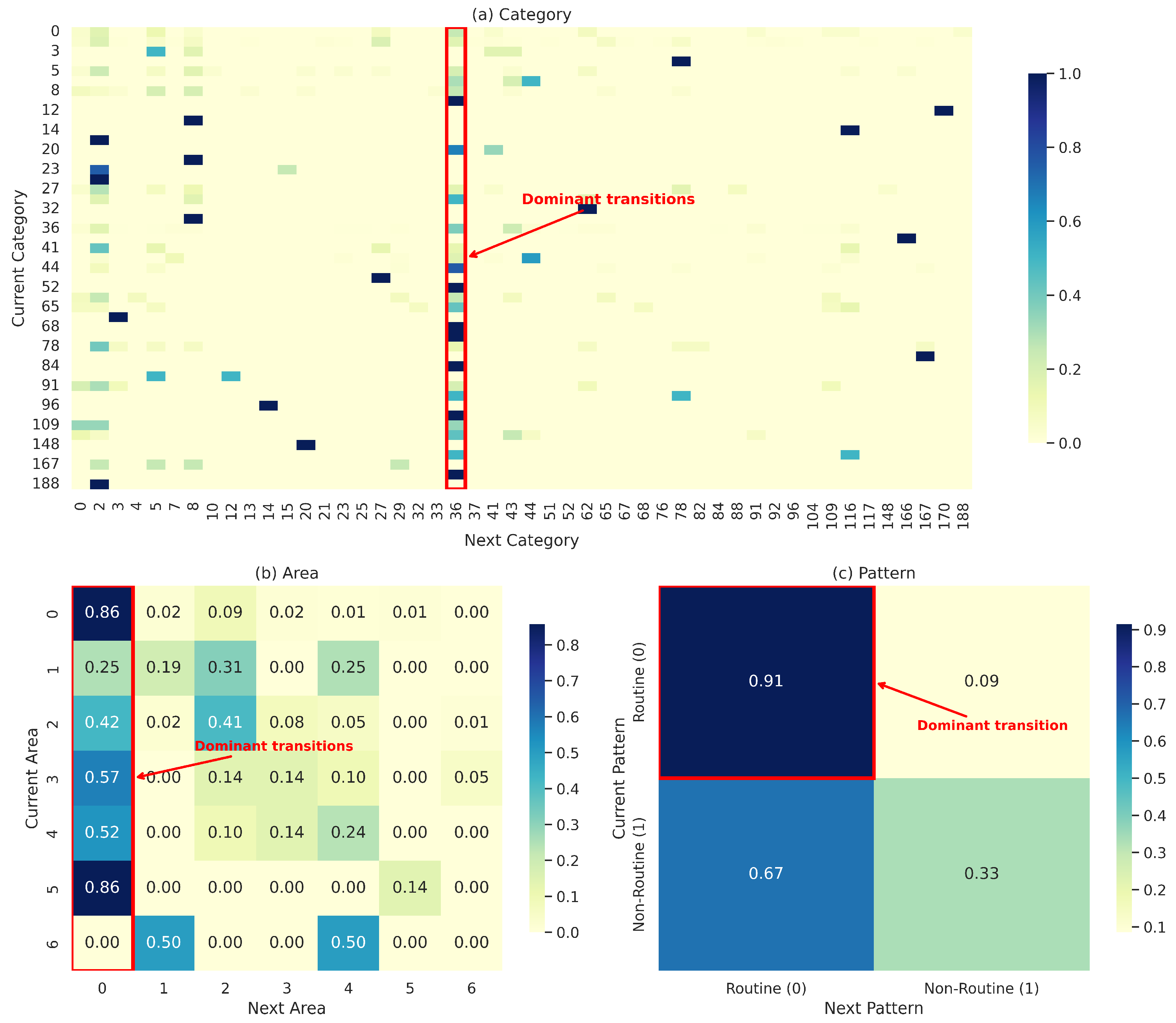
Recent studies have emphasized the need for incorporating multiple contextual features—such as category, spatial area, and temporal factors—to enhance prediction robustness under real-world conditions. Category transitions have proven effective for modeling semantic relationships between locations, while spatial clustering captures the geographical distribution of user movements. User behavioral patterns further reveal regularities that cannot be captured solely by spatial or categorical attributes. Frameworks such as AFNextPOI [8] integrate pattern-based features with area information, demonstrating improved performance by leveraging complementary contextual signals. However, existing methods often lack a unified mechanism to jointly model heterogeneous features and explicitly model transition awareness between the current and next POIs. While transition-aware models have significantly advanced next POI recommendation, most existing approaches still focus on a limited set of features, making them vulnerable to incomplete or sparse check-in data. Prior studies have seldom examined how category, area, and routine/non-routine patterns correlate between consecutive locations. Our analysis shows distinct dependencies, with patterns being the most deterministic, yet such feature-level relationships remain underexplored for improving next location prediction.

Figure 1 illustrates the relationships between check-in points from multiple perspectives. Only specific points, such as Figure 1a category 36, Figure 1b area 0, and Figure 1c the routine pattern, demonstrate a high likelihood of exhibiting relational dependence.

3. Problem Definition

3.1. Definition of Uncertain Check-In

Uncertain check-in refers to a location record whose spatial or temporal attributes are ambiguous, inaccurate, or missing, making it difficult to represent the user’s true movement path. In addition, a check-in can also be considered uncertain when its behavioral pattern deviates from the user’s normal routine, indicating irregular or unexpected mobility behavior.

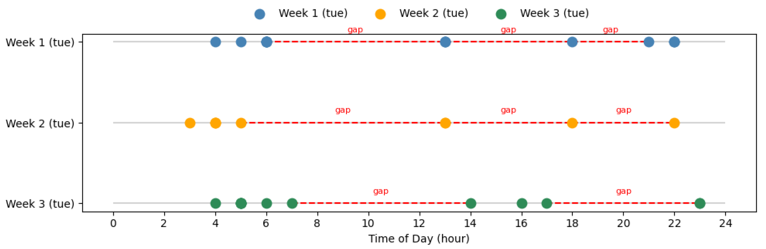
In location-based social networks (LBSNs), user trajectories often contain incomplete or inconsistent information due to irregular check-in behavior. Such uncertainty may arise from factors including missing check-ins between consecutive locations, GPS noise, incorrect timestamps, or user behavior that deviates from habitual mobility patterns. These uncertain points introduce noise and discontinuity into the trajectory, leading to degraded model performance in sequential prediction. Therefore, handling uncertain check-ins effectively is crucial for building reliable next POI recommendation models, especially when working with real-world datasets that are sparse and irregularly sampled. Figure 2 illustrates a user check-in timeline on the same weekday across different weeks. Each line represents the same user’s check-in behavior on Tuesday across three different weeks. The dashed red lines indicate long temporal gaps (>2 h) between consecutive check-ins, reflecting missing records and temporal sparsity even within the same weekday pattern.

3.2. Problem of Uncertain Check-In

To address uncertainty in user trajectories, recent studies, such as the AHLTP model [15], focus on predicting hidden or missing locations within a user’s trajectory. By leveraging both venue classifications and sequential trajectory patterns, the model infers potentially unrecorded check-ins and predicts future locations, thereby enhancing the accuracy of mobility forecasting in LBSN applications. This approach provides valuable insights into handling trajectory incompleteness, suggesting that incorporating data imputation or hidden-location prediction into future POI prediction frameworks could further improve model robustness and adaptability. Unlike models that attempt to infer hidden or missing check-ins, our proposed multi-feature framework learns the contextual correlations underlying user mobility. Inferring hidden locations requires strong assumptions about users’ intentions and continuous transitions, which are often unreliable under real-world conditions where data sparsity and noise prevail. In contrast, our multi-feature learning design mitigates the limitations of missing or uncertain check-ins by modeling users’ latent mobility preferences rather than explicitly reconstructing the missing points. This representation captures the underlying contextual dependencies among features, enabling the model to produce more robust and accurate predictions under trajectory uncertainty. As a result, it outperforms hidden-location inference methods that are often prone to noise, while maintaining high performance even with incomplete or irregular trajectories.

4. Methodology

4.1. Data Preprocessing

We assessed the performance of our model on two real-world datasets: Foursquare check-ins in New York (NYC) and Tokyo (TKY), collected between 12 April 2012 and 16 February 2013. Originally, this dataset was used to explore spatial–temporal regularities in user behavior in location-based social networks (LBSNs) [16].

The preprocessing procedure followed the same protocol as the comparison models, including the removal of duplicate and noisy records. Duplicate check-ins were defined as records generated by the same user at the same location within the same hour on the same day, and were removed to eliminate redundancy. Locations with fewer than 10 check-ins were regarded as unpopular and excluded to reduce data sparsity and filter out locations with insufficient interaction records. Such locations provide limited behavioral information and may introduce noise into the modeling process, thereby negatively affecting the learning of reliable mobility patterns.

Similarly, we filtered out trajectories with fewer than 10 check-ins and users with fewer than three trajectories to ensure sufficient behavioral records for modeling user mobility patterns and to reduce sparsity caused by extremely short trajectories or inactive users. Finally, we organized the data by user and performed a sequential split based on the temporal order of check-ins, using the first 80% of each user’s trajectory for training and the remaining 20% for testing. The dataset descriptions are provided in

Table 2. Dataset Description.

Feature	NYC		TKY
	Original	After Prep.	Original	After Prep.
#user	1083	379	2293	1148
#category	398	236	385	225
#check-ins	227,428	67,547	573,703	228,852

.

The summary of all the important notations in this paper is listed below in

Table 3. Notation and Descriptions.

Notation	Description
$U\in \{u_1,u_2,u_3,\dots ,u_{\left|U\right|}\}$	Set of users
$L\in \{l_1,l_2,l_3,\dots ,l_{\left|l\right|}\}$	Set of latitude and longitude pairs
$C\in \{c_1,c_2,c_3,\dots ,c_{\left|C\right|}\}$	Set of categories
$hr$	Set of hours $\{0,1,2,\dots ,23\}$
d	Set of days of week $\{0,1,2,\dots ,6\}$
$c(u,i)$	Category of candidate i for user u
$a(u,i)$	Area of candidate i for user u
$pt(u,i)\in \{R,N\}$	Indicates whether the point is routine (R) or non-routine (N)
$p(u,i)$	Vector $[l,c,h,d]$ of candidate i for user u
P	Vector $[l,c,h,d]$ of candidate i for all points
$tra(u,i)$	Trajectory of sequence i for user u is represented by category feature.
$s(u,i)$	Sequence of candidate i for user u
$h(u,i)$	Hidden state of candidate i for user u

.

4.2. MTF-POI Framework

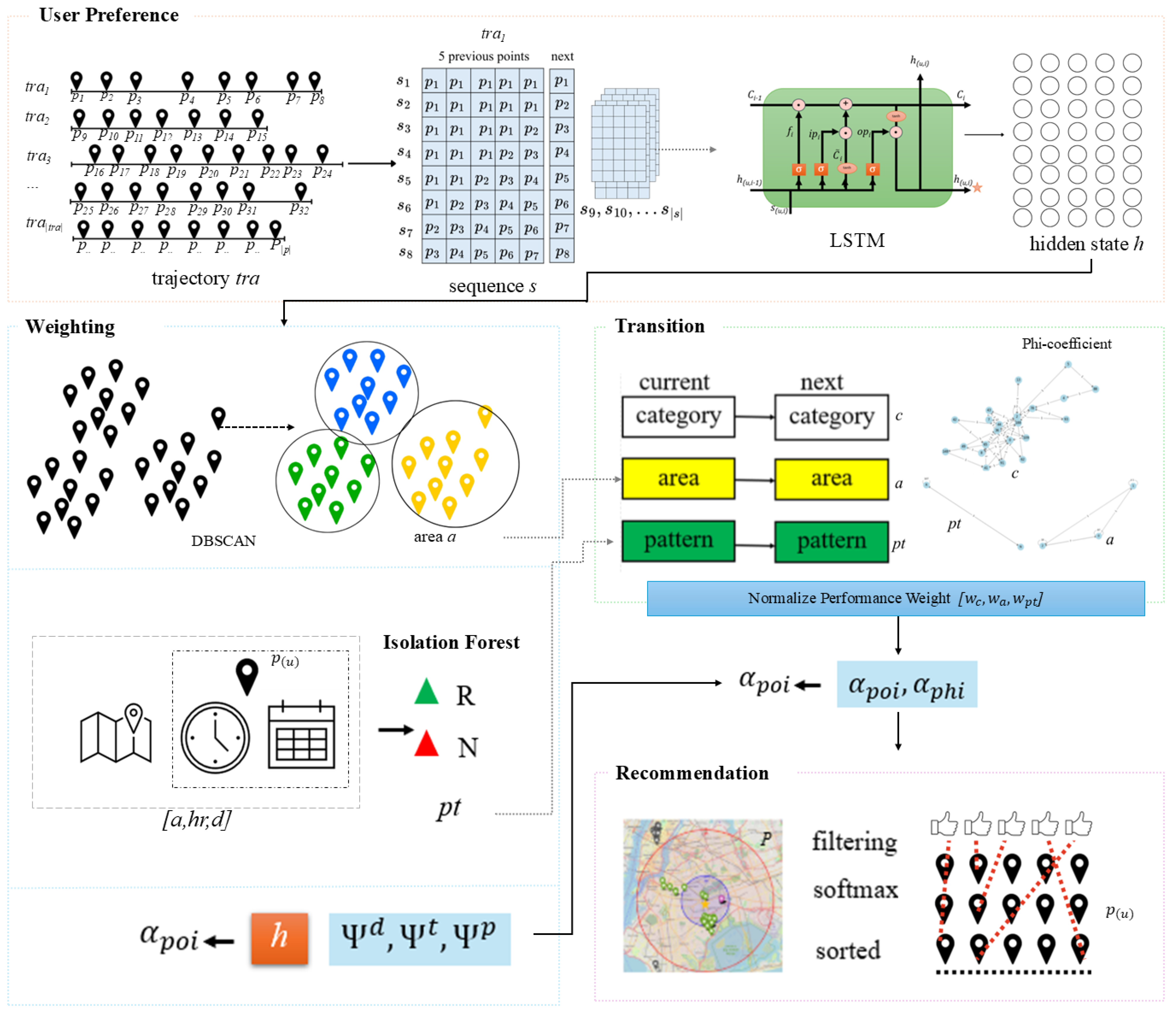
We propose the MTF-POI framework, which is structured into four layers, as illustrated in Figure 3. These four interconnected layers collaboratively transform raw user check-in data into accurate Next Point-of-Interest recommendations. The first layer, the Embedded (User Preference) Layer, focuses on modeling sequential user behavior by transforming historical check-in trajectories into ordered sequences and learning temporal dependencies using an LSTM network. The hidden state output represents the user’s latent mobility preference in the current context. The second layer, the Preference Identification and Weighting Layer, captures spatial and behavioral characteristics by clustering POIs into geographic areas using DBSCAN and identifying routine and non-routine movement patterns through training based on contextual features such as area, hour, and day. These components generate adaptive preference weights that reflect the user’s spatial familiarity and behavioral regularity. The third layer, the Transition Modeling Layer, explicitly models transitions across multiple dimensions, including category-to-category, area-to-area, and pattern-to-pattern movements. The strength of these transitions is quantified using the Phi-coefficient, enabling the framework to emphasize meaningful movement correlations while suppressing weak or noisy relationships. Finally, the Recommendation Layer integrates user preferences and transition scores to produce ranked POI recommendations by filtering candidate locations, normalizing scores with a softmax function, and sorting the results to return the Top-K recommended POIs. This four-layer architecture enables the effective integration of temporal, spatial, categorical, and behavioral information, resulting in robust, personalized Next-POI recommendations.

4.2.1. User Preference

To construct user trajectories, we segmented check-in data into individual sequences by splitting the trajectory whenever the time gap between consecutive check-ins exceeded 24 h. For each resulting trajectory, we applied a sliding window of length 5 to generate input sequences for the next-location prediction. We shifted the sequence by one position at a time until reaching the final check-in of the trajectory [17]. The entire sequence s was input to the LSTM model as categorical data to generate the hidden state for the next point, as shown in Equations (1)–(3).

$$h_{(u,i)}=o{p}_i\odot tanh\left(C_i\right)$$

(1)

$$C_i=f_i\odot C_{(i-1)}+i{p}_i\odot \widetilde{C_i}$$

(2)

$$o{p}_i=\sigma \left(W_o·[h_{(i-1)},s_i]+b_o\right)$$

(3)

where:

• $h_{(u,i)}$ denotes the hidden state at time step i for user u.
• $o_i$ represents the output gate activation at time step i.
• ⊙ indicates element-wise multiplication.
• tanh denotes the hyperbolic tangent activation function.
• $C_i$ refers to the new cell state, combining the forgotten part of the past state and the new information.
• $f_i$ is the forget gate activation.
• $i_p$ denotes the input gate activation at time step i.
• $\widetilde{C_i}$ represents the candidate values used to update the cell state.
• $\sigma$ denotes the sigmoid activation function.
• $W_o$ refers to the weight matrix for the output gate.
• $b_o$ is the bias term for the output gate.
• $h_{(i-1)}$ is the hidden state from the previous step.
• $s_i$ is the input index of category c at the current time step i.

We employed early stopping or, alternatively, trained for a maximum of 200 epochs for each user-specific model within a Python-based computational framework implemented on top of Python 3.12.12 and TensorFlow/Keras 2.12.0. The hidden size is intentionally set to 1 to produce a compact temporal representation of the input sequence. Each timestep is represented by a single scalar feature (embedding size = 1), and no embedding layer is applied. A fully connected dense layer with one neuron is used as the output layer. No dropout is applied, given the minimal architecture designed to prevent overfitting on sparse data. The network processes the entire input sequence and outputs the final hidden state of the last timestep, which is then passed to a fully connected Dense layer for regression.

4.2.2. Weighting

The objective of this task is to learn a weight that reflects both the distance d and the time t from the current location. We computed the distance d between the current point and the next candidate point using the Haversine formula [18]. The distance d is used to compute the weights of candidate points, as defined in Equation (4). The time difference t, computed between the current time and that of each candidate point, is used to assign weights to all candidates, as shown in Equation (5).

$${\mathrm{\Psi }}_{(u,i)}^d={\displaystyle \frac{exp(\alpha ·d_i)}{{\sum }_{j=1}^{|h_u|}exp(\alpha ·d_j)}}$$

(4)

$${\mathrm{\Psi }}_{(u,i)}^t={\displaystyle \frac{exp(\alpha ·t_i)}{{\sum }_{j=1}^{|h_u|}exp(\alpha ·t_j)}}$$

(5)

The parameter $\alpha$ is set to $-1$ based on a preliminary grid search over $\alpha \in \{-3,-2,-1,-0.5,-0.1\}$ on two datasets. As shown in

Table 4. Recall@1 on the validation sets for different values of $\alpha$.

Dataset	$\mathit{\alpha }=-3$	$\mathit{\alpha }=-2$	$\mathit{\alpha }=-1$	$\mathit{\alpha }=-0.5$	$\mathit{\alpha }=-0.1$
NYC	0.2401	0.2401	0.2480	0.2296	0.2243
TKY	0.2422	0.2439	0.2474	0.2404	0.1943

Note: The bold values indicate the best performance, corresponding to $\alpha =-1$.

, $\alpha =-1$ achieves the best Recall@1 by providing a balanced trade-off: values closer to 0 reduce the discriminative power of the distance/time penalty, while more negative values overly suppress moderately distant but potentially relevant candidates. This analysis is conducted on the validation sets of both the NYC and TKY datasets, where similar trends are consistently observed.

For candidate check-in points, we applied different weightings based on the pattern. ${\mathrm{\Psi }}_{(u,i)}^p$ denotes the pattern-aware weight assigned to the i-th check-in of user u. When the current check-in is classified as a routine pattern, and its area belongs to the user’s frequently visited areas $\left(po{p}_{\left(u\right)}^a\right)$, the weight is maximized to 2. Similarly, if the check-in is non-routine, but its category is contained in the user’s popular categories $\left(po{p}_{\left(u\right)}^c\right)$ [8], the weight is also set to 2 because it still reflects the user’s stable preferences. For all remaining cases, the weight is set to  1 to avoid suppressing potentially valid locations. The weighting criteria are defined in Equation (6).

$${\mathrm{\Psi }}_{(u,i)}^p=\left\{\begin{array}{cc}2,\hfill & \mathrm{if}p{t}_{(u,i)}=R\mathrm{and}{a}_{(u,i)}\in po{p}_{\left(u\right)}^a\hfill \\ 2,\hfill & \mathrm{if}p{t}_{(u,i)}=N\mathrm{and}{a}_{(u,i)}\in po{p}_{\left(u\right)}^c\hfill \\ 1,\hfill & \mathrm{otherwise}\hfill \end{array}\right.$$

(6)

where

• $po{p}_{\left(u\right)}^a$ denotes the set of popular areas for user u.
• $po{p}_{\left(u\right)}^c$ denotes the set of popular categories for user u.

The exponent term ${\mathrm{\Psi }}_{(u,i)}^p$ acts as a pattern-aware amplification factor. This mechanism allows the model to highlight POIs adaptively with reliable temporal–spatial–behavioral consistency, as shown in Equation (7).

$${\alpha }_{poi}={\left(h_{(u,i)}+{\mathrm{\Psi }}_{(u,i)}^d+{\mathrm{\Psi }}_{(u,i)}^t\right)}^{{\mathrm{\Psi }}_{(u,i)}^p}$$

(7)

4.2.3. Transition

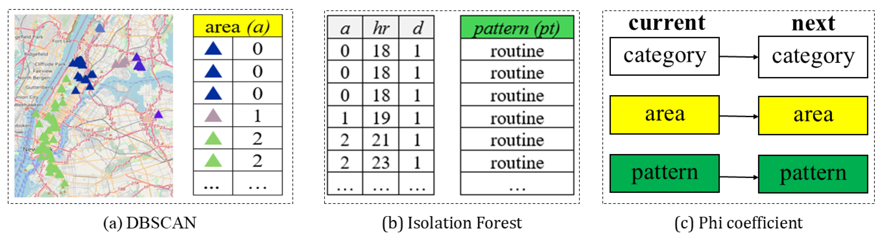
We clustered user areas using DBSCAN (Density-Based Spatial Clustering of Applications with Noise) [19] from $p\left(u\right)$. The result is represented in Figure 4a. Subsequently, we use a, $hr$, and d to identify user patterns using the training algorithm [20], as illustrated in Figure 4b. In the final step, category c, area a, and pattern $pt$ are used to measure their correlation with the next candidate using the Phi coefficient, as illustrated in Figure 4c. An overview of the process in this step is illustrated in Figure 4.

DBSCAN: The area a is partitioned using the DBSCAN algorithm, where $N_{\epsilon }\left(p\right)$ denotes the set of neighboring points within a radius $\epsilon$ of point p.The parameter $\epsilon$ represents the radius distance in DBSCAN, determining whether other points are close enough to be considered neighbors of the point in the dataset $p_{(u,i)\left[l\right]}$. The function $\mathrm{dist}(p,q)$ denotes the distance between points p and q, as defined in Equation (8). The notation $|N_{\epsilon }\left(p\right)|$ in Equation (9) indicates the number of neighboring points. The DBSCAN parameters were determined as follows. The radius $\epsilon$ was selected based on k-distance graph analysis [21]. The elbow point in the sorted nearest-neighbor distance plot consistently appeared near $\epsilon =0.5$ for both datasets, indicating a natural density boundary for location clusters. As shown in

Table 5. Nearest-neighbor distance statistics and DBSCAN parameters.

Dataset	Mean NN (km)	Median NN (km)	$\mathit{\epsilon }$ (km)	minPts
NYC	0.080	0.030	$\approx 0.5$	2
TKY	0.053	0.023	$\approx 0.5$	2

, the median nearest-neighbor distance is approximately 0.03 km for NYC and 0.02 km for TKY, indicating the high spatial density of urban POIs. Therefore, $\epsilon =0.5$ was selected as an appropriate clustering radius, as it aligns with the density structure of the datasets while capturing neighborhood-scale spatial clusters.

We set $\mathrm{MinPts}=2$ as the minimum viable threshold given the sparse nature of LBSN check-in data. Larger values caused the majority of locations to be classified as noise, eliminating meaningful spatial patterns. This setting is consistent with prior work on spatial clustering for LBSN data. The density-reachable relationship among core points $(p_1,p_2,p_3,\dots ,p_n)$ is expressed in Equation (10).

$$N_{\epsilon }\left(p\right)=\{q\in p_{(u,i)\left[l\right]}\mid \mathrm{dist}(p,q)\le \epsilon \}$$

(8)

$$|N_{\epsilon }\left(p\right)|\ge \mathrm{MinPts}$$

(9)

$$p_1=p,p_n=q,p_{i+1}\in N_{\epsilon }\left(p_i\right)$$

(10)

Isolation forest: The vector $x=[a,hr,d]$ represents the spatial area, hour, and day features, which serve as inputs to the anomaly detection training algorithm. The resulting anomaly score is either 1 or $-1$, indicating whether a check-in point is classified as a Routine or Non-routine check-in point. A threshold value $\theta$ is applied to separate the anomaly scores, which are determined based on an expected outlier ratio of 0.1, as shown in Equations (11)–(13). The training is configured with $n\_estimators=100$, which provides a sufficient ensemble size for stable anomaly detection in low-dimensional datasets. This configuration is appropriate for the relatively small feature space (three features) and the per-user training subsets in the NYC and TKY datasets, which range from 30 to 2399 records depending on the length of each user’s activity history. The model uses a contamination parameter of 0.1 to represent the expected proportion of anomalies, and a fixed random state of 42 to ensure reproducibility.

$$x=[a,hr,d]$$

(11)

$$s(x,n)=2{\displaystyle \frac{h\left(x\right)}{c\left(n\right)}}$$

(12)

$$y\left(x\right)=\left\{\begin{array}{cc}-1,\hfill & \mathrm{if}s(x,n)\ge \theta \left(\mathrm{Non}\text{-}\mathrm{routine}\right)\hfill \\ +1,\hfill & \mathrm{if}s(x,n)<\theta \left(\mathrm{Routine}\right)\hfill \end{array}\right.$$

(13)

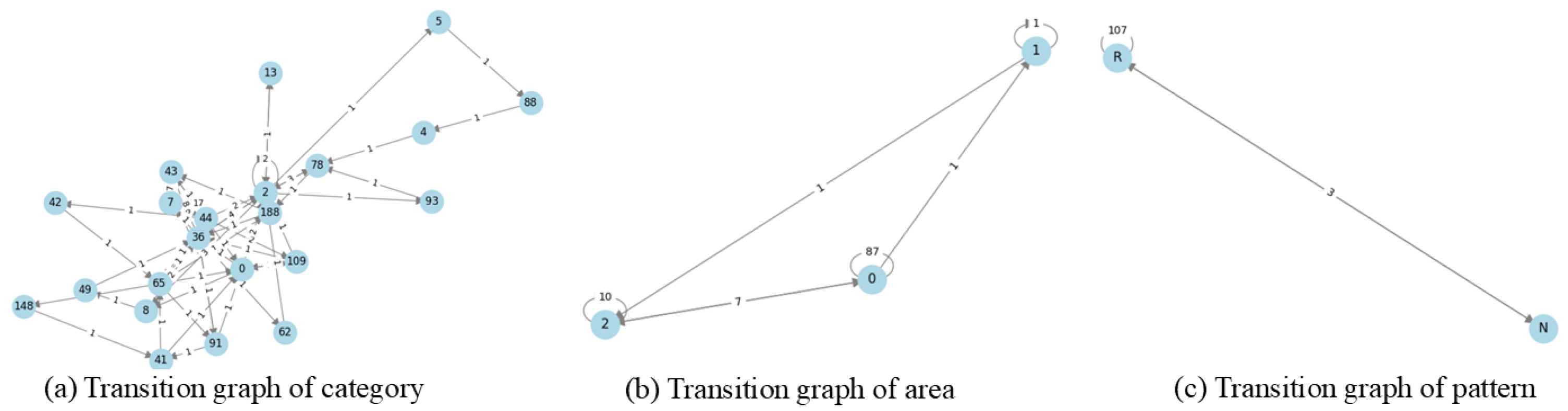
Phi Coefficient: The transition of relations for category, area, and pattern is shown in Figure 5. Each node represents a location, while the arrows indicate transitions between locations. The number on each arrow denotes the frequency of the movement. Furthermore, phi coefficient is shown in Equation (14) by the condition of the current and next location for all check-in points.

The phi coefficient measures the relationship under three vector conditions. A result of $\varphi =1$ indicates a perfect positive relationship, $\varphi =-1$ indicates a complete negative relationship, and $\varphi =0$ indicates no relationship.

$$\varphi (\mathrm{current}\_\mathrm{loc},\mathrm{next}\_\mathrm{loc})={\displaystyle \frac{ad-bc}{\sqrt{(a+b)(c+d)(b+d)}}}$$

(14)

where

• a is the number of times where the current location = 1 and next location = 1.
• b is the number of times where the current location = 1 and next location = 0.
• c is the number of times where the current location = 0 and next location = 1.
• d is the number of times where the current location = 0 and next location = 0.

The score is computed as the weighted average w of phi coefficients across all check-ins in the training set, as defined in Equation (15). When no prior co-occurrence exists between check-in features, the phi coefficient is set to 0. The summary of ${\alpha }_{poi}$ score is presented in Equation (16).

$${\alpha }_{phi}={\displaystyle \frac{{\sum }_{i=1}^{\left|\varphi \right|}({\varphi }_i·w_i)}{{\sum }_{i=1}^{\left|w\right|}{w}_i}}$$

(15)

where

• $\varphi =[{\varphi }_c,{\varphi }_a,{\varphi }_{pt}]$ represents the phi coefficients for category, area, and pattern features.
• $w=[w_c,w_a,w_{pt}]$ represents the Normalized Performance Weights: NPWs assigned to each $\varphi$ component. The NPW computation in Section 4.3.1 produces weights that capture the relative effectiveness of each feature for each experimental dataset.

Finally, the overall ${\alpha }_{poi}$ score is updated as follows:

$${\alpha }_{poi(u,i)}={\alpha }_{poi(u,i)}+{\alpha }_{phi(u,i)}$$

(16)

4.2.4. Recommendation

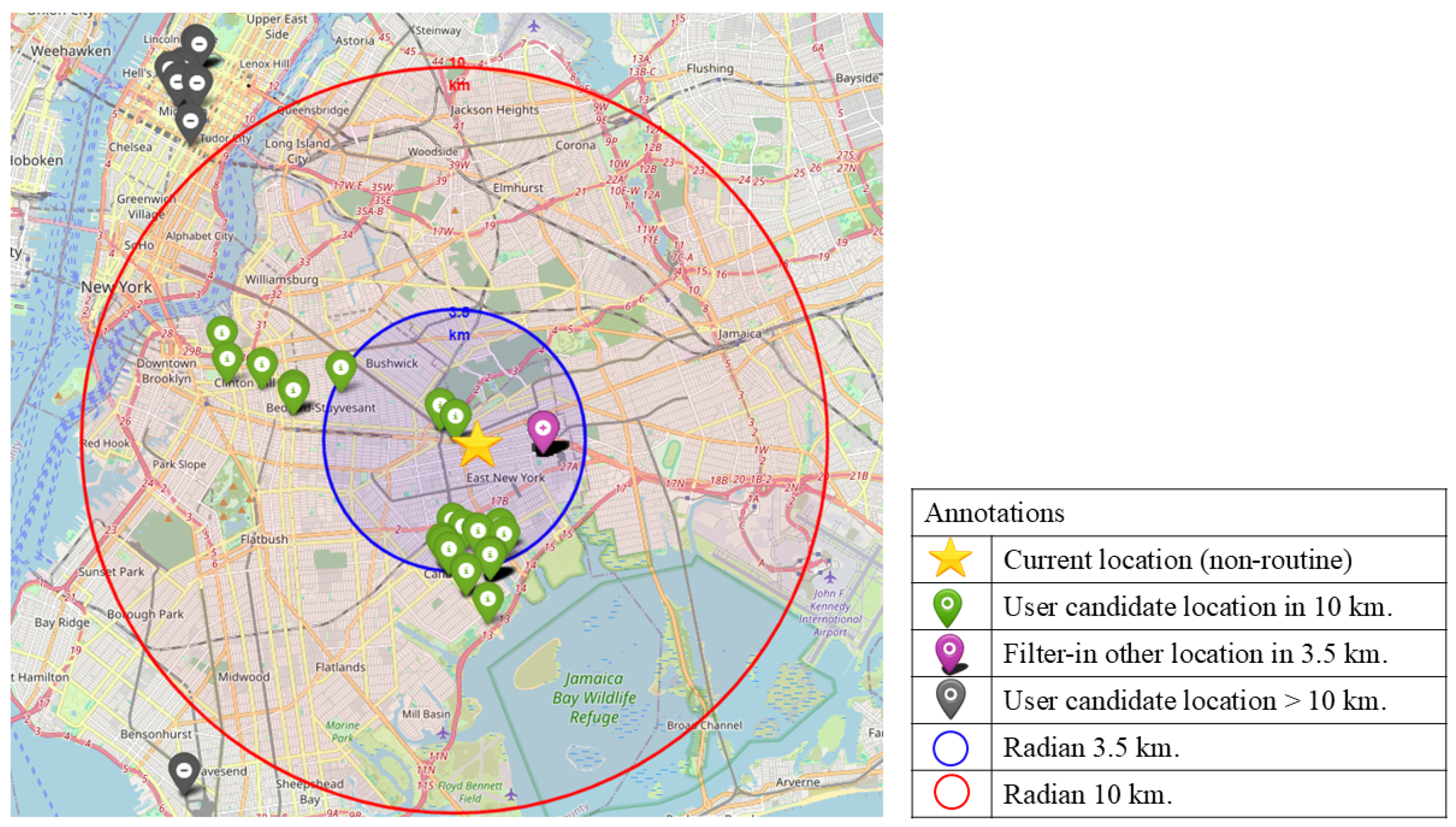
We selected alternative locations from P within a 3.5 km radius of the user’s next location, matching the user’s preferred categories at that time, specifically when the user was in a non-routine pattern. The model assigns the highest score to these selected check-in points for the user. Otherwise, the method filters points based on the user’s average score, as shown in Algorithm 1. To eliminate distant locations, the algorithm assigns the minimum score to any candidate beyond 10 km, as shown in Algorithm 2. The candidate points of the user are explored in Figure 6.

We used the Softmax function to compute output probabilities, where e is the exponentiation of each element to ensure positivity, and the resulting values sum to 1 as shown in Equation (17). In the final step, we sort the candidate points by score and retrieve the top@K ranked locations.

$$\mathrm{Softmax}\left({\alpha }_{poi(u,i)}\right)={\displaystyle \frac{e^{{\alpha }_{poi(u,i)}-max\left({\alpha }_{poi\left(u\right)}\right)}}{{\sum }_{i=1}^n{e}^{{\alpha }_{poi(u,i)}-max\left({\alpha }_{poi\left(u\right)}\right)}}}$$

(17)

where

• ${\sum }_{i=1}^n{\alpha }_{poi(u,i)}=1$ ensures that all output probabilities sum to one.
• n denotes the total number of candidate ${\alpha }_{poi\left(u\right)}$ values.

4.3. Experiment

We evaluated the performance of all methods using standard metrics, namely Recall@K and NDCG@K, based on the top-K recommended POIs for each user [22], where $K=\{1,3,5\}$. Equations (18)–(20) define these evaluation metrics.

$$\mathrm{Recall}@\mathrm{K}={\displaystyle \frac{1}{\left|U\right|}}\sum _{u=1}^{\left|U\right|}{\displaystyle \frac{{\mathrm{Recall}}_u@K(r_u\cap t_u)}{|t_u|}}$$

(18)

where

• $r_u$ is the set of top-K POIs recommended for user u.
• $t_u$ is the set of ground-truth POIs actually visited by user u at the next location in the test set.

$$\mathrm{NDCG}@\mathrm{K}={\displaystyle \frac{1}{\left|U\right|}}\sum _{u=1}^{\left|U\right|}{\displaystyle \frac{{\mathrm{DCG}}_u@K}{{\mathrm{IDCG}}_u@K}}$$

(19)

$${\mathrm{DCG}}_u@K=\sum _{i=1}^N{\displaystyle \frac{2^{re{l}_i}-1}{{log}_2(i+1)}}$$

(20)

where

• $\mathrm{IDCG}$ is the maximum possible DCG for a given recommendation list.
• $\mathrm{DCG}$ (Discounted Cumulative Gain) measures the quality of ranked results.
• $re{l}_i$ denotes the relevance score of the item at position i.
• N is the number of correctly recommended POIs.

Algorithm 1: Filter-In Cross-User Candidate POIs Based on the User’s Popular Categories

Require:  User u; current check-in $(l_u,h{r}_u)$;   1: user u’s historical check-ins $p_u$;   2: check-in log of other users P;   3: radius threshold r (e.g., $3.5$ km);   4: time similarity threshold ${\tau }_{hr}$;   5: preference scoring function $p_u[l_i,h{r}_i,c_i).score$ = ${\alpha }_{poi(u,i)}$ Ensure:  Filtered candidate POI set with scores $f{n}_{cat}$   6: Initialize $f{n}_{cat}\leftarrow \varnothing$   7: Compute user popular categories under the current time context:   8: $po{p}_u\leftarrow \mathrm{POPULARCATEGORY}(u,h{r}_u,p_u)$   9: Compute user average and maximum preference scores: 10: ${\overline{s}}_u\leftarrow \mathrm{AVERAGESCORE}(u,p_u)$ 11: $s_u^{max}\leftarrow \mathrm{MAXSCORE}(u,p_u)$ 12: for all check-in $(i,l_i,h{r}_i,c_i)$ in P do 13:       $d\leftarrow \mathrm{GEODISTANCE}(l_u,l_i)$ 14:       $\mathrm{\Delta }t\leftarrow \mathrm{TIMEGAP}(h{r}_u,h{r}_i)$ 15:       if $d\le r$ and $\mathrm{\Delta }t\le {\tau }_{hr}$ and $c_i\in po{p}_u$ then 16:           if $l_i\in p_u$ then 17:              ${\alpha }_{poi(u,i)}\leftarrow s_u^{max}$                  ▹ duplicate with user’s own POI: assign max score 18:           else 19:              ${\alpha }_{poi(u,i)}\leftarrow {\overline{s}}_u$                                 ▹ new cross-user POI: assign average score 20:           end if 21:           $f{n}_{cat}\leftarrow f{n}_{cat}\cup \left\{(l_i,s_i)\right\}$                                       ▹ filter-in this POI with its score 22:       end if 23: end for 24: $f{n}_{cat}\leftarrow \mathrm{UNIQUEPOISWITHMAXSCORE}\left(f{n}_{cat}\right)$ 25: return ${\alpha }_{poi(u,i)}$

Algorithm 2: Filter-Out Low-Preference and Distant POIs from User History

Require:  User u; current check-in $(l_u,h{r}_u)$;   1: user u’s historical check-ins $p_u$;   2: maximum distance threshold $R_{max}$ (e.g., 10 km);   3: minimum score $s_u^{min}$ Ensure:  Filtered personal POI set with scores $p_u.score={\alpha }_{poi(u,i)}$   4: Compute user average preference score: ${\overline{s}}_u\leftarrow \mathrm{AVERAGESCORE}(u,p_u)$   5: Initialize $f{n}_u\leftarrow \varnothing$   6: for all check-in $(j,l_j,h{r}_j,c_j)$ in $p_u$ do   7:       $d_j\leftarrow \mathrm{GEODISTANCE}(l_u,l_j)$   8:       if $d_j>R_{max}$ then   9:           ${\alpha }_{poi(u,i)}\leftarrow s_u^{min}$      ▹ eliminate distant locations by assigning a minimum score 10:           continue                                                            ▹ do not include this POI in $f{n}_u$ 11:       end if 12: end for 13: return ${\alpha }_{poi(u,i)}$

4.3.1. Feature Effectiveness and Synergy in Multi-Feature Transitions

We compared our model under different feature configurations in the process coefficient. Specifically, four model variants are evaluated: MTF-c, which incorporates only category features; MTF-a, which integrates area features; MTF-pt, which emphasizes user check-in pattern features; and the full MTF-POI model, which combines all features (category, area, and pattern) into a unified framework.

The experimental results are presented in

Table 6. Comparison of model performance with coefficients from different feature configurations.

Metric	NYC Dataset				TKY Dataset
	MTF-c	MTF-a	MTF-pt	MTF-POI	MTF-c	MTF-a	MTF-pt	MTF-POI
Recall@1	0.1715	0.2084	0.1662	0.2480	0.1655	0.2300	0.2021	0.2474
Recall@3	0.2801	0.3799	0.3522	0.3712	0.3116	0.3955	0.3801	0.4232
Recall@5	0.4112	0.4634	0.4409	0.4902	0.4158	0.5144	0.4945	0.5390
NDCG@1	0.1715	0.2084	0.1662	0.2480	0.1655	0.2300	0.2021	0.2474
NDCG@3	0.2203	0.2919	0.2606	0.3007	0.2370	0.3161	0.2958	0.3371
NDCG@5	0.2724	0.3251	0.2959	0.3482	0.2779	0.3634	0.3412	0.3827

Note: Ablation study Recall and NDCG performance under single-feature vs. multi-feature configurations on NYC and TKy datasets. Underlined values indicate the best single-feature performance; bold values denote the full-feature version (MTF-POI).

. It can be observed that integrating multiple features yields better overall performance, as the combined model (MTF-POI) consistently outperforms the individual feature-based variants across all evaluation metrics.

The area-based variant (MTF-a) achieves the best performance among single-feature models, outperforming both the category-based (MTF-c) and pattern-based (MTF-pt) configurations across all evaluation metrics. This finding confirms that spatial correlation is a dominant factor influencing user mobility and that clustering POIs into representative areas enables the model to better capture users’ movement tendencies within geographically coherent regions.

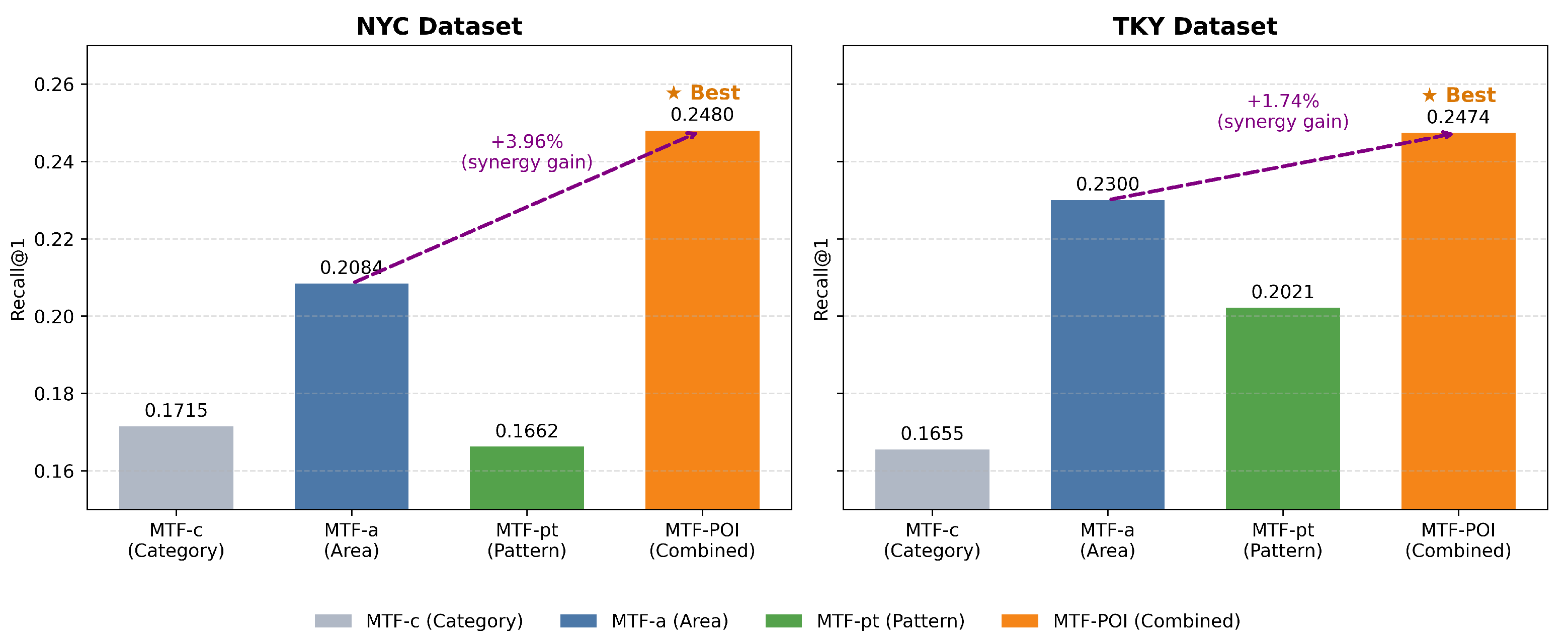
More importantly, the combined model (MTF-POI) that integrates category, area, and pattern features yields the highest accuracy overall. Specifically, Recall@1 increases from 0.2084 (MTF-a) to 0.2480 for NYC and from 0.2300 to 0.2474 for TKY, indicating an additional gain of +3.96 and +1.74 percentage points, respectively. This improvement highlights a synergistic interaction among the three features: the area feature provides spatial stability, the category feature contributes semantic context, and the pattern feature refines temporal and behavioral consistency. Together, they enable the model to precisely predict the most probable next POI at the top-1 rank while maintaining steady gains in higher K metrics (Recall@3, Recall@5, and NDCG).

(a)

Total Performance Score: TPS

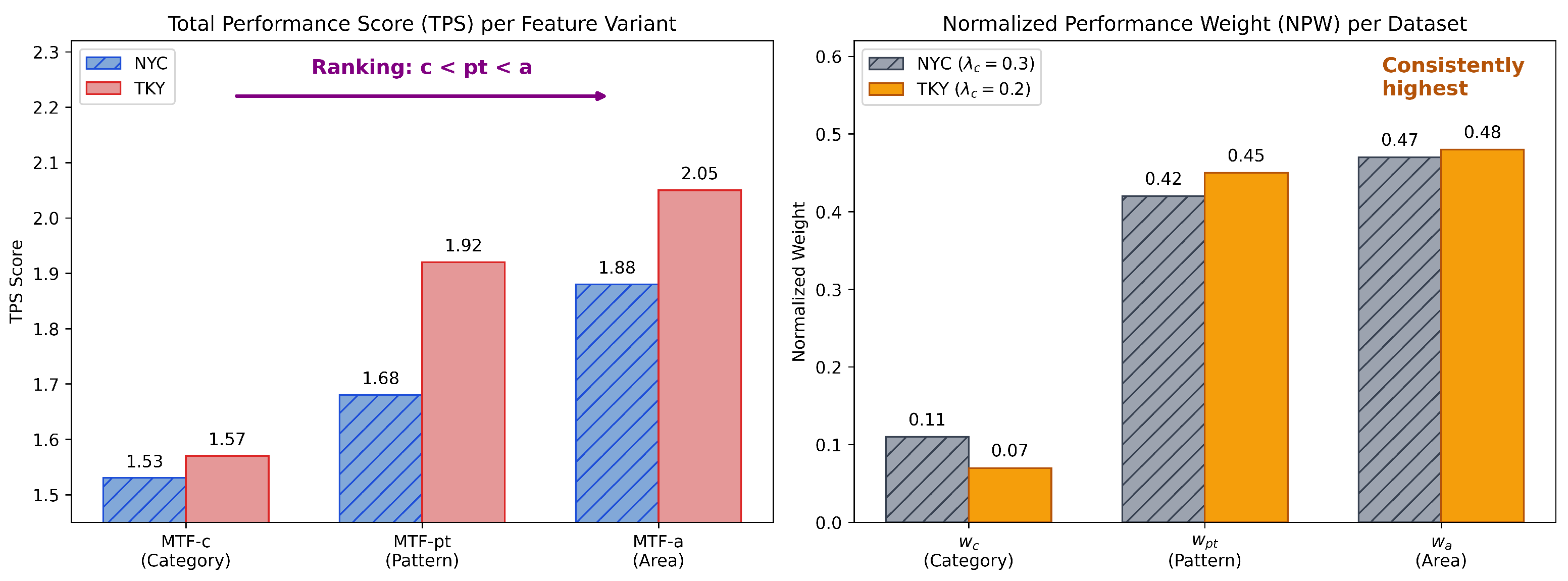
The $TP{S}_f^{\left(d\right)}$ in Equation (21) was introduced to provide an integrated evaluation of model performance across multiple metrics and datasets. Specifically, the $TP{S}_f^{\left(d\right)}$ reveals consistent performance trends across feature configurations. Among the evaluated variants, MTF-a achieves the highest TPS on both the NYC and TKY datasets, resulting in the largest overall TPS score. The ordering of TPS values (MTF-a > MTF-pt > MTF-c) remains stable across both datasets, demonstrating the robustness of feature importance rankings and reinforcing the generalizability of the proposed feature design. Overall, these results validate the effectiveness of incorporating richer contextual and temporal signals to enhance the next POI prediction performance.

$$TP{S}_f^{\left(d\right)}=\sum _{k\in \{1,3,5\}}\left(\mathrm{Recall}@k_f^{\left(d\right)}+\mathrm{NDCG}@k_f^{\left(d\right)}\right)$$

(21)

(b)

Normalized Performance Weight: NPW

The $NP{W}_f^{\left(d\right)}$, as defined in Equation (22), quantifies the relative contribution of each feature by integrating its predictive performance across both datasets and all evaluation metrics. First, the score $NP{W}_f^{\left(d\right)}$ is computed separately for each dataset by averaging the $TP{S}_f^{\left(d\right)}$ scores over the evaluation cutoffs k. This results in a unified performance score that reflects the overall effectiveness of feature $f\in \{c,a,pt\}$.

$$NP{W}_f^{\left(d\right)}={\displaystyle \frac{1}{6}}\sum _{k\in \{1,3,5\}}\left(TP{S}_f^{\left(d\right)}\right)$$

(22)

(c)

The penalty factor

The weight $w_f$ is then obtained by normalizing $S_f$ with respect to the total score of all features, ensuring that the weights are comparable and collectively sum to one. Finally, the constraint $w_c+w_a+w_{pt}=1$ guarantees that the category, area, and pattern features together account for the full proportion of the performance contribution of the model, as Equations (23) and (24).

$$w_f={\displaystyle \frac{S_f^{\prime }}{S_c^{\prime }+S_a^{\prime }+S_{pt}^{\prime }}}{S}_c^{\prime }={\lambda }_c·S_c$$

(23)

$$w_c+w_a+w_{pt}=1$$

(24)

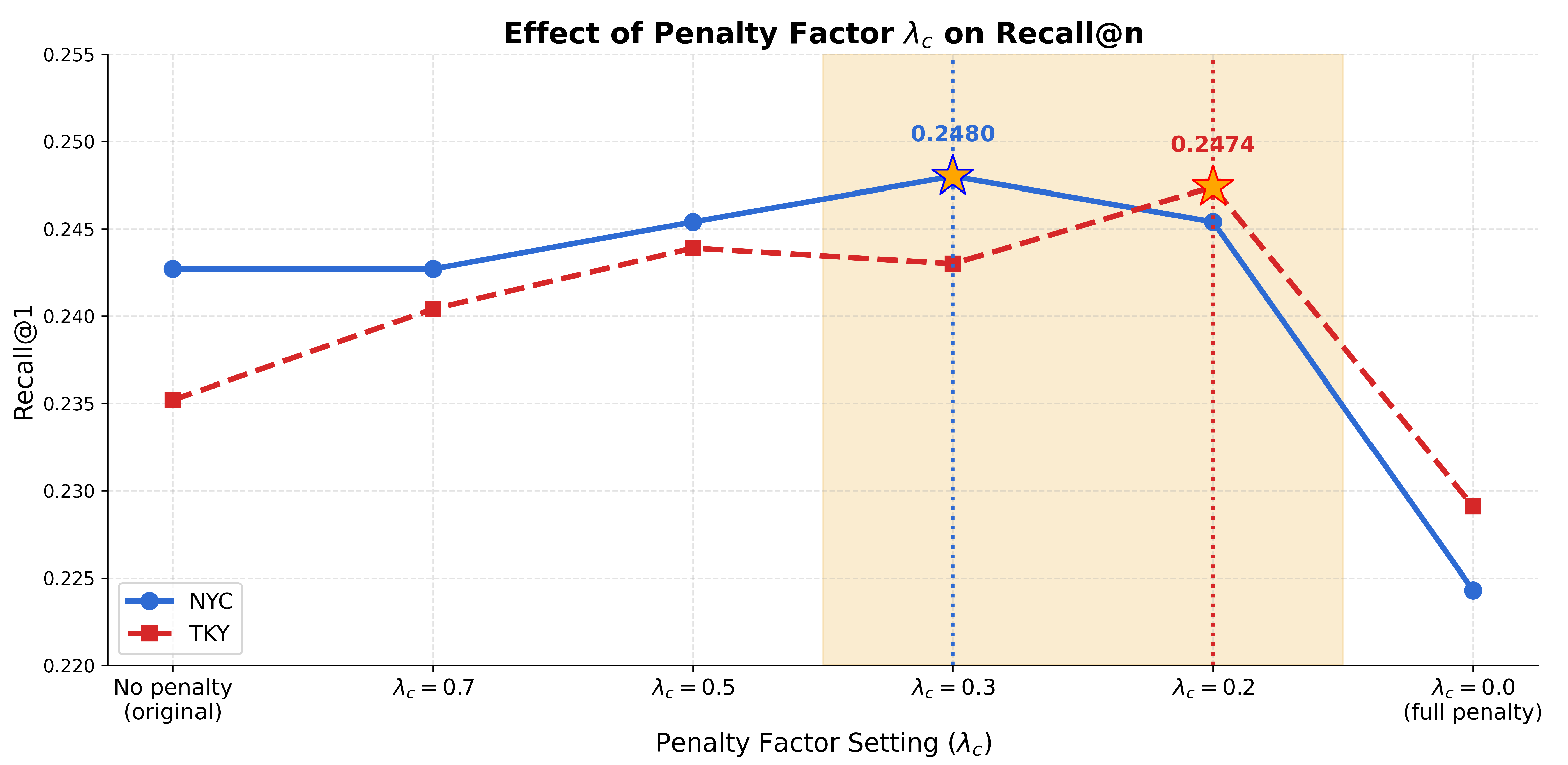
The model introduces a penalty factor to balance the contribution of different features. This design is consistent with feature weighting strategies, in which features are assigned different levels of importance based on their relevance to representing the underlying patterns [23]. The value of ${\lambda }_c$ is determined empirically to achieve stable performance. Overall, the results in

Table 7. Effect of penalty factor ${\lambda }_c$ on recommendation performance.

${\mathit{\lambda }}_{\mathit{c}}$	NYC						TKY
	R@1	R@3	R@5	N@1	N@3	N@5	R@1	R@3	R@5	N@1	N@3	N@5
1	0.2427	0.3654	0.4981	0.2427	0.2932	0.3461	0.2352	0.4045	0.5211	0.2352	0.3210	0.3673
0.7	0.2427	0.3615	0.4928	0.2427	0.2912	0.3438	0.2404	0.4106	0.5241	0.2404	0.3263	0.3713
0.5	0.2454	0.3720	0.4902	0.2454	0.2987	0.3454	0.2439	0.4130	0.5338	0.2439	0.3297	0.3775
0.3	0.2480	0.3712	0.4902	0.2480	0.3007	0.3482	0.2430	0.4244	0.5409	0.2430	0.3354	0.3814
0.2	0.2454	0.3755	0.4945	0.2454	0.3024	0.3498	0.2474	0.4232	0.5390	0.2472	0.3371	0.3827
0	0.2243	0.3905	0.4939	0.2243	0.3033	0.3443	0.2291	0.4133	0.5359	0.2291	0.3259	0.3745

indicate that a moderate penalty factor ($0.2\le {\lambda }_c\le 0.3$) improves top-ranked recommendation quality while maintaining stable performance across other metrics. As Recall@1 represents the most stringent evaluation scenario—where the model must correctly predict the next POI as the top-ranked recommendation—we selected the configuration that yields the highest Recall@1 performance. However, the optimal value of ${\lambda }_c$ may vary across datasets and should be tuned according to their specific characteristics, such as data distribution and mobility patterns.

Figure 7 illustrates the effect of varying ${\lambda }_c$ on Recall@1 for both the NYC and TKY datasets. The results reveal that the optimal ${\lambda }_c$ differs across datasets: NYC achieves peak performance at ${\lambda }_c=0.3$ (Recall@1 = 0.2480), while TKY peaks at ${\lambda }_c=0.2$ (Recall@1 = 0.2474). This discrepancy is not unexpected and reflects fundamental differences in the mobility characteristics of the two cities.

Specifically, the optimal ${\lambda }_c$ is governed by the degree of category transition noise in each dataset. NYC exhibits higher category diversity (236 active categories after preprocessing) with more dispersed visit distributions, producing noisier category transition signals that require stronger penalization (${\lambda }_c=0.3$) to prevent low-quality features from dominating the multi-feature score. TKY, while containing 225 categories, displays more concentrated activity in specific venue types driven by regular commuting behavior, resulting in slightly more informative category transitions that benefit from a milder penalty (${\lambda }_c=0.2$).

These observations suggest that ${\lambda }_c$ should be interpreted as a dataset-sensitive hyperparameter rather than a universal constant. To reflect the cross-dataset generality of the framework, results in

Table 8. TPS and NPW values of different features for NYC and TKY datasets.

Feature	NYC			TKY
	TPS	NPW	NPW (${\mathit{\lambda }}_{\mathit{c}}$ = 0.3)	TPS	NPW	NPW (${\mathit{\lambda }}_{\mathit{c}}$ = 0.2)
$W_c$ (Category)	1.53	0.30	0.11	1.57	0.28	0.07
$W_a$ (Area)	1.88	0.37	0.47	2.05	0.37	0.48
$W_{p}t$ (Pattern)	1.68	0.33	0.42	1.92	0.35	0.45

are reported using dataset-specific optimal values: ${\lambda }_c=0.3$ for NYC and ${\lambda }_c=0.2$ for TKY with NPW computation.

Feature synergy analysis shows the Total Performance Score for each feature variant and the normalized Performance weights for the NYC and TKY datasets. The ranking $c<pt<a$ indicates that the area feature consistently provides the highest contribution, while the normalized weights further confirm that $w_a$ receives the largest weight across both datasets, as presented in Figure 8.

4.3.2. Performance Comparison with Baselines

We compared our proposed framework, MTF-POI, with several widely used baseline methods for Next Point-of-Interest (Next-POI) recommendation. First, the evaluation is conducted exclusively on the Foursquare NYC and TKY datasets. This choice is deliberate for two reasons: (1) all baseline models compared in this study were originally benchmarked on these datasets, ensuring fair and reproducible comparison under identical experimental conditions; and (2) the proposed framework requires per-user sequential check-in trajectories that include co-located timestamps, GPS coordinates, and category labels to support area clustering (DBSCAN) and behavioral pattern detection (Isolation Forest).

Despite evaluating on a single platform, the use of two geographically and behaviorally distinct cities—New York City and Tokyo—provides a meaningful degree of cross-context validation. The two datasets exhibit contrasting mobility regimes: NYC is characterized by high venue diversity, spatially dispersed POI distributions, and irregular user schedules, while TKY displays concentrated commuting flows, higher behavioral regularity, and more predictable daily routines. This structural contrast ensures that findings are not specific to a single mobility pattern.

• LSTM [24]: A Python-based integrated computational framework built on TensorFlow/Keras is designed for sequential data, similar to our model.
• GRU [25]: A Python-based integrated computational framework built on TensorFlow/Keras is designed for sequential data, similar to our model.
• LSTPM [3,5]: A model that addresses the limitations of existing POI recommendation methods by incorporating both long-term and short-term user preferences.
• RTPM [5]: A model that analyzes long-term and short-term user preferences, real-time user behaviors, probability estimation, and recommendation modules.
• AFNextPOI [8]: A framework that categorizes user travel patterns into different cases and applies distinct evaluation methods for each, enabling better handling of data uncertainty.
• MTF-POI (Proposed): The proposed framework extends AFNextPOI by integrating multi-feature transition awareness between the current and next locations.

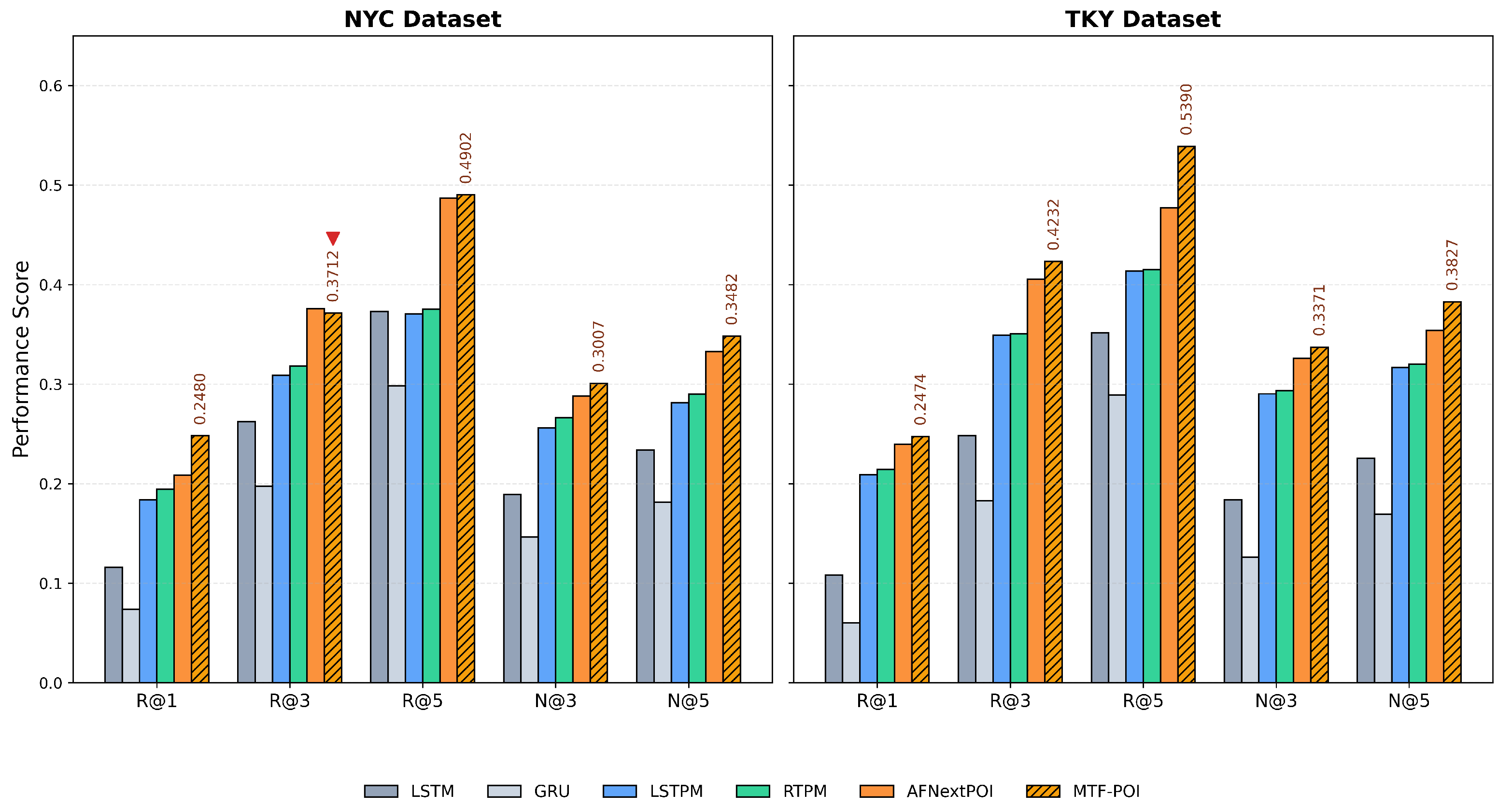
Results from the proposed methodology and baseline comparisons are presented in

Table 9. Result of experiment with baseline Next POI model.

Model	NYC Dataset					TKY Dataset
	R@1	R@3	R@5	N@3	N@5	R@1	R@3	R@5	N@3	N@5
LSTM	0.1161	0.2621	0.3730	0.1891	0.2337	0.1080	0.2480	0.3514	0.1837	0.2255
GRU	0.0739	0.1974	0.2983	0.1462	0.1814	0.0601	0.1828	0.2891	0.1262	0.1694
LSTPM	0.1836	0.3087	0.3707	0.2559	0.2814	0.2088	0.3492	0.4135	0.2902	0.3168
RTPM	0.1944	0.3182	0.3752	0.2663	0.2898	0.2143	0.3504	0.4151	0.2934	0.3201
AFNextPOI	0.2084	0.3755	0.4869	0.2878	0.3328	0.2395	0.4055	0.4771	0.3260	0.3539
MTF-POI	0.2480	0.3712	0.4902	0.3007	0.3482	0.2474	0.4232	0.5390	0.3371	0.3827
Improv.	+19.01%	−1.14%	+0.68%	+4.48%	+4.63%	+3.30%	+4.36%	+12.98%	+3.41%	+8.15%

Note: Performance comparison of MTF-POI with baseline Next-POI models on the NYC and TKY datasets. Our proposed model is shown in bold, and the best results are underlined.

. Experiments on two real-world datasets demonstrate that the proposed framework consistently achieves strong performance, particularly in top-1 accuracy (Recall@1) and ranking quality (NDCG). Notably, MTF-POI outperforms all baseline methods on the TKY dataset across all evaluation metrics. On the NYC dataset, while the proposed model achieves the best Recall@1 and NDCG scores, its performance on Recall@3 is slightly lower than AFNextPOI. These results suggest that the proposed framework is more effective in capturing precise next-location intent, especially for top-ranked recommendations. This behavior aligns with the design of the multi-feature transition modeling, which prioritizes precise next-step prediction over broader candidate ranking. Baseline results are partially taken from our previous work [8].

Performance comparison between MTF-POI and baseline models on the NYC and TKY datasets is shown in Figure 9. MTF-POI generally achieves the best performance across most metrics, particularly for Recall@1 and all NDCG metrics on both datasets. The bars corresponding to MTF-POI are highlighted with a hatch pattern, while the symbol ▾ indicates cases where MTF-POI performs slightly lower than AFNextPOI (NYC: R@3).

We assessed statistical significance using the Wilcoxon signed-rank test to determine whether differences in model performance are significant. Effect size is measured using Cliff’s $\delta$, which quantifies the magnitude of the difference in performance between two methods. Additionally, a 95% confidence interval (CI) is computed as Equation (25).

$$CI=\overline{x}\pm 1.96{\displaystyle \frac{s}{\sqrt{n}}},$$

(25)

where $\overline{x}$ denotes the sample mean, s represents the standard deviation, and n is the sample size.

Table 10. Statistical comparison between MTF-POI and AFNexPOI on NYC and TKY datasets.

Dataset	Metric	MTF  Avg	AFNexPOI Avg	p-Value	Cliff’s $\mathit{\delta }$	95% CI
NYC	Recall@1	0.2480	0.2084	0.0321	0.0396	[0.0026, 0.0792]
	NDCG@1	0.2480	0.2084	0.0321	0.0396	[0.0053, 0.0765]
	Recall@3	0.3712	0.3755	0.7680	−0.0029	[−0.0435, 0.0343]
	NDCG@3	0.3007	0.2878	0.6096	0.0116	[−0.0215, 0.0449]
	Recall@5	0.4902	0.4869	0.9712	0.0034	[−0.0409, 0.0431]
	NDCG@5	0.3482	0.3328	0.2134	0.0109	[−0.0125, 0.0419]
TKY	Recall@1	0.2474	0.2395	0.4913	0.0078	[−0.0140, 0.0296]
	NDCG@1	0.2474	0.2395	0.4913	0.0078	[−0.0140, 0.0296]
	Recall@3	0.4232	0.4055	0.2703	0.0180	[−0.0060, 0.0423]
	NDCG@3	0.3371	0.3260	0.2395	0.0155	[−0.0083, 0.0295]
	Recall@5	0.5390	0.4771	$<0.001$	0.0653	[0.0369, 0.0889]
	NDCG@5	0.3827	0.3539	0.0006	0.0454	[0.0102, 0.0477]

Note: Statistical significance test results (Wilcoxon singed-rank) and effect sizes (Cliff’s $\delta$) comparing MTF-POI vs. AFNextPOI.

shows that, for the NYC dataset, MTF-POI achieves statistically significant improvements in both Recall@1 and NDCG@1 ($p=0.0321$), indicating a stronger ability to accurately identify the correct next POI at the top recommendation position. This result suggests that the multi-feature modeling strategy effectively captures complex user mobility behaviors in dense urban environments such as New York City, where user movements are highly diverse and context-dependent. Although the improvements in Recall@3, NDCG@3, Recall@5, and NDCG@5 are not statistically significant, MTF-POI still maintains competitive, and often slightly higher, average performance, demonstrating stable recommendation quality across different ranking thresholds.

For the TKY dataset, MTF-POI shows statistically significant improvements in Recall@5 ($p<0.001$) and NDCG@5 ($p=0.0006$), indicating a clear advantage in ranking relevant POIs within the top-5 recommendation list.

This suggests that the proposed model is particularly effective in capturing broader candidate POIs within structured mobility patterns such as those commonly observed in Tokyo. The results imply that integrating heterogeneous mobility features enables MTF-POI to better model both short-term and contextual user preferences.

The overall statistical significance across metrics was further examined using Fisher’s combined probability test. The aggregated result for the NYC dataset yields $p\approx 0.10$, indicating that the overall performance difference between MTF-POI and AFNexPOI is not statistically significant across all metrics. In contrast, the TKY dataset shows a significant combined result ($p\approx 0.0002$), suggesting that MTF-POI provides a statistically significant overall improvement over AFNexPOI.

4.3.3. Influence of Multifeature Feature Transition

The consistent superiority of MTF-POI across both datasets demonstrates that multi-feature transition awareness generalizes effectively under different spatial densities and urban structures. Hence, integrating all three correlated features not only enhances overall recall and ranking quality, but also strengthens the model’s adaptability to both routine and non-routine user behaviors.

The bar chart in Figure 10 presents a comparison of Recall@1 performance across four model versions (MTF-c, MTF-a, MTF-pt, and MTF-POI) on two datasets (NYC and TKY). Each dataset has four groups of bars, representing the performance of the different version.

From the results, MTF-POI consistently achieves the highest Recall@1 in both datasets. Among the three versions (MTF-c, MTF-a, and MTF-pt), MTF-a consistently achieves the highest Recall@1 on both the NYC and TKY datasets. This indicates that the feature-enhanced version (MTF-a) performs better than the category-based (MTF-c) and pattern-based (MTF-pt) versions. By combining the three features and applying a weighted average for scoring, the performance is further improved compared to the MTF-POI version.

The contrasting results of MTF-pt between NYC and TKY reflect differences in mobility regularity and city structure. In the NYC dataset, MTF-pt performs slightly worse than MTF-c because the routine/non-routine pattern signal is not strongly correlated with the actual next-location transitions. NYC exhibits high mobility diversity, with users frequently visiting new places, changing routes dynamically, and having irregular schedules. As a result, binary pattern-type labels (routine vs. non-routine) provide little predictive power and may even introduce noise, leading MTF-pt to underperform regarding the simpler category-based feature.

In contrast, TKY displays much more structured and repeatable mobility behavior, driven by predictable commuting flows, concentrated activity zones, and higher regularity in daily routines. In such an environment, pattern-type information becomes highly valuable: whether a movement is routine or non-routine strongly influences the likelihood of the next POI. This makes MTF-pt substantially outperform MTF-c in the TKY dataset.

4.3.4. TPS Statistical Validation

Spearman’s rank correlation coefficient ($\rho$) was used to measure the monotonic association between TPS rankings and the individual evaluation metrics. As defined in Equation (26), this coefficient quantifies the monotonic relationship between two ranked variables [26].

$$\rho =1-{\displaystyle \frac{6\sum d_i^2}{n(n^2-1)}}$$

(26)

where $d_i$ denotes the difference between the ranks of the paired observations and n is the number of samples.

Kendall’s rank correlation coefficient ($\tau$) was also used to assess the ordinal association between TPS rankings and individual evaluation metrics. As defined in Equation (27), Kendall’s $\tau$ measures the difference between the number of concordant and discordant pairs [26,27].

$$\tau ={\displaystyle \frac{C-D}{\frac{n(n-1)}{2}}}$$

(27)

Figure 11 shows the rank correlation analysis between TPS and individual evaluation metrics across the NYC and TKY datasets. The first two heatmaps show the rank matrices of model variants across Recall, NDCG, and TPS metrics, with rank 1 indicating the best performance. The third heatmap shows the Spearman correlation between TPS and individual metrics, demonstrating moderate to perfect rank consistency.

The Spearman ($\rho$) and Kendall ($\tau$) correlations between the Total Performance Score (TPS) ranking and the individual evaluation metrics across feature configurations for both datasets are shown. Overall, these results indicate that TPS provides a consistent aggregated indicator of model performance across multiple evaluation metrics presented in

Table 11. Spearman ($\rho$) and Kendall ($\tau$) correlations between TPS ranking and individual metrics across feature configurations.

Metric	NYC Dataset				TKY Dataset
	$\mathit{\rho }$	$\mathit{\tau }$	p-Value	Interpret.	$\mathit{\rho }$	$\mathit{\tau }$	p-Value	Interpret.
Recall@1	0.800	0.667	0.2000	Moderate	1.000	1.000	$<0.001$	Perfect
Recall@3	0.800	0.667	0.2000	Moderate	1.000	1.000	$<0.001$	Perfect
Recall@5	1.000	1.000	$<0.001$	Perfect	1.000	1.000	$<0.001$	Perfect
NDCG@1	0.800	0.667	0.2000	Moderate	1.000	1.000	$<0.001$	Perfect
NDCG@3	1.000	1.000	$<0.001$	Perfect	1.000	1.000	$<0.001$	Perfect
NDCG@5	1.000	1.000	$<0.001$	Perfect	1.000	1.000	$<0.001$	Perfect

.

For the NYC dataset, moderate correlations are observed for Recall@1, Recall@3, and NDCG@1 ($\rho =0.800$, $\tau =0.667$), indicating slight differences in ranking compared with TPS. In contrast, Recall@5, NDCG@3, and NDCG@5 exhibit perfect rank agreement ($\rho =1.000$, $\tau =1.000$). For the TKY dataset, all metrics show perfect correlations with TPS, suggesting that the TPS ranking fully aligns with the rankings produced by the individual metrics.

4.3.5. Influence of Hidden Location Attraction

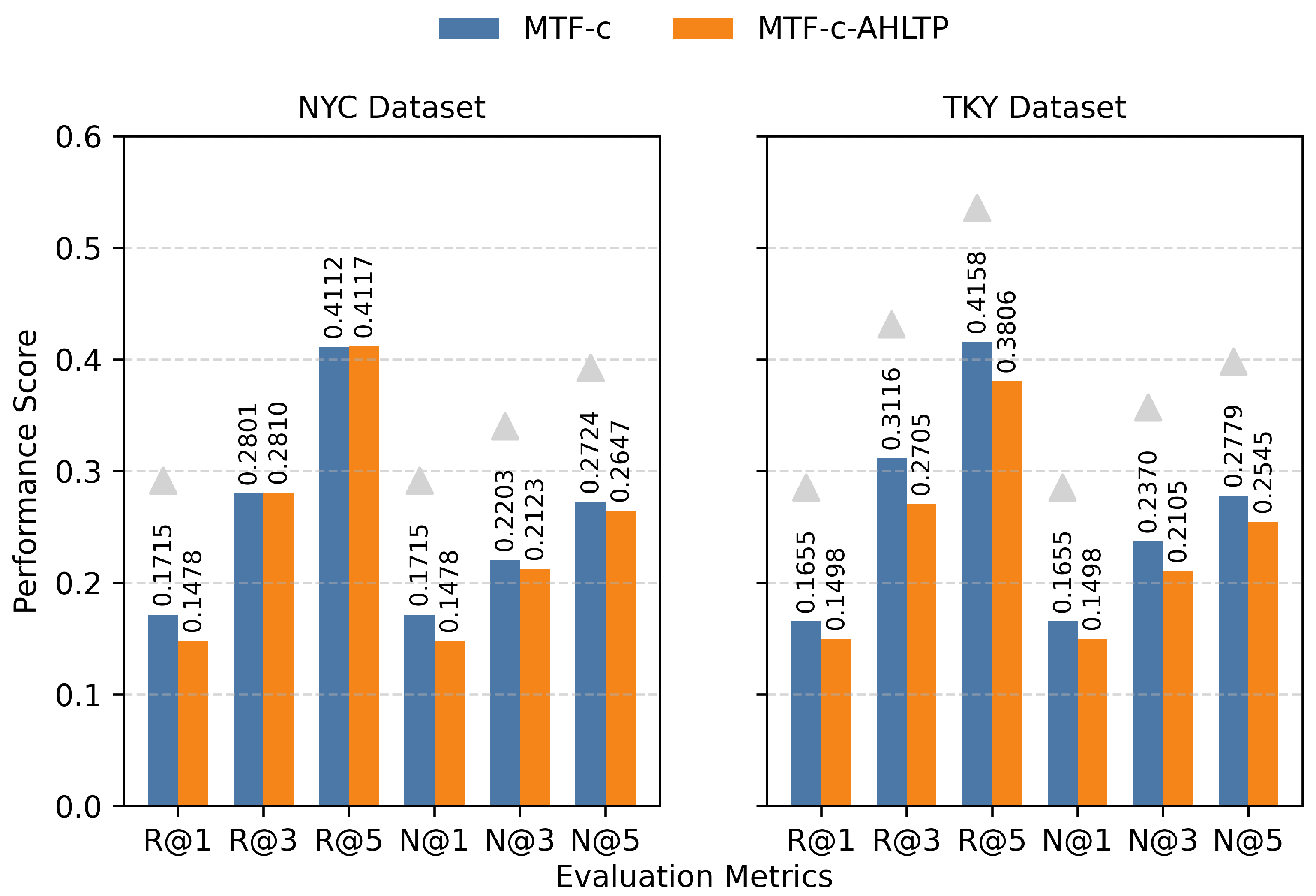
The MTF-c-AHLTP follows the same modeling process as MTF-c, where next-POI prediction is based on category transitions. The key difference is that MTF-c-AHLTP augments user trajectories with hidden locations inferred from category associations using the AHLTP [15] approach prior to model training.

The comparison between MTF-c and MTF-c-AHLTP in Figure 12 shows that incorporating hidden locations does not improve top-rank accuracy or ranking quality. While MTF-c-AHLTP slightly increases candidate coverage at higher K values, it introduces noise into category transitions, leading to lower Recall@1 and NDCG@K. These results suggest that, for large-scale next POI prediction, using only real check-in transitions is more effective than augmenting trajectories with inferred locations.

More importantly, this result indicates that addressing uncertain check-ins through feature transfer is more effective than explicitly inserting inferred locations into user trajectories. Rather than modifying the original trajectory structure, feature transfer enables the model to adaptively reweight or transform existing features based on contextual and behavioral information, thereby mitigating uncertainty without amplifying error propagation. In contrast, insertion of hidden location alters transition sequences by introducing inferred check-ins that may not reflect the user’s true short-term intent, leading to poor ranking performance.

These findings suggest that, for large-scale next-POI prediction, modeling uncertainty at the feature level provides a more robust solution than augmenting trajectories with inferred locations.

4.4. Time Complexity Analysis

This section analyzes the computational complexity of the proposed framework by decomposing it into four main components.

Let n denote the sequence length, d the embedding dimension, f the number of feature types, and m the number of candidate POIs. The Computational complexity of each component is presented in

Table 12. Computational complexity of each component in the proposed framework.

Component	Time Complexity	Space Complexity
Sequence Modeling	$O\left(n^{2}d\right)$	$O(n^2+nd)$
Feature Verification	$O\left(nf\right)$	$O\left(nf\right)$
Transition Modeling	$O\left(nm\right)$	$O\left(m\right)$
Multi-Feature Integration	$O\left(nfd\right)$	$O(nd+nf)$
Recommendation	$O(nmlogk)$	$O\left(m\right)$
Overall Complexity	$\begin{array}{c}O(n^{2}d+nf+nm+nfd+nmlogk)\hfill \end{array}$	$\begin{array}{c}O(n^2+nd+nf+m)\hfill \end{array}$

.

The dominant term is $O\left(n^{2}d\right)$ from sequence modeling. Other components scale linearly with respect to n, indicating that the additional feature processing introduces limited computational overhead while improving recommendation performance.

Table 13. Computational complexity comparison between the proposed model and baseline methods.

Model	Time Complexity	Space Complexity
LSTM	$O(n·d^2+nmlogk)$	$O(nd+d^2+m)$
GRU	$O(n·d^2+nmlogk)$	$O(nd+d^2+m)$
LSTPM	$O(n·d^2+nm+nmlogk)$	$O(nd+d^2+m)$
RTPM	$O(n·d^2+nm+nmlogk)$	$O(nd+d^2+m)$
AFNextPOI	$O(n^2·d+nf+nm+nmlogk)$	$O(n^2+nd+2m)$
MTF-POI (Proposed)	$O(n^2·d+nf+nm+nfd+nmlogk)$	$O(n^2+2nd+2nf+2m)$

shows that the proposed MTF-POI introduces additional feature-related computations compared with baseline models. However, most components scale linearly with respect to the number of features and locations, while the dominant term remains $O(n^2·d)$, similar to AFNextPOI. Therefore, the overall computational complexity remains manageable while enabling richer multi-feature modeling.

5. Discussion and Limitations

The performance differences observed in Table 9 can be explained by how each component of the proposed framework interacts with user mobility characteristics. In particular, improvements in top-rank accuracy are closely related to how short-term intent and contextual uncertainty are handled across layers, rather than to the reconstruction of missing trajectory points.

At the sequence level, the LSTM-based preference layer captures temporal dependencies among consecutive check-ins, providing a compact representation of users’ recent mobility context. This representation reduces sensitivity to sporadic or irregular check-ins and allows the model to focus on short-term decision patterns. In contrast, models that directly operate on augmented trajectories may propagate uncertainty introduced earlier, especially when inferred locations are not aligned with users’ immediate intent.

The weighting layer further influences performance by differentiating candidate POIs according to spatial and behavioral contexts. Area-based clustering enables the model to emphasize movements within frequently visited regions, while the distinction between routine and non-routine patterns adjusts the influence of regular and exploratory behaviors. This mechanism helps explain why the proposed approach remains stable under heterogeneous user behaviors, whereas methods that rely on fixed trajectory structures are more affected by noisy or ambiguous check-ins.

Differences in ranking quality are mainly attributable to the transition layer. By integrating category, area, and pattern transitions and refining their contributions using the Phi coefficient, the model selectively amplifies meaningful correlations while suppressing weak or spurious ones. This explains the observed gains in NDCG@K, as relevant POIs are more likely to be ranked higher when multiple contextual signals consistently support the transition.

A notable contrast can be observed between MTF-c and MTF-c-AHLTP. Although augmenting trajectories with hidden locations slightly increases candidate coverage at higher K values, it also alters category transition distributions by introducing inferred check-ins. These inferred transitions may not correspond to users’ actual short-term choices, leading to degraded top-rank accuracy and ranking quality. This comparison suggests that uncertain check-ins are better handled through feature-level adaptation across layers than through explicit trajectory augmentation.

A few limitations of the current study should be acknowledged. First, the evaluation is conducted exclusively on Foursquare datasets from a single provider. Although NYC and TKY represent contrasting mobility regimes in terms of venue diversity, spatial density, and behavioral regularity, cross-platform validation on structurally compatible datasets remains an important direction. Future work will prioritize adapting the framework to additional LBSN datasets as they become available. Second, the penalty factor ${\lambda }_c$ requires dataset-specific tuning, as the optimal value differs between NYC and TKY, which limits plug-and-play applicability without additional validation. Finally, while MTF-POI achieves statistically significant improvements in top-1 accuracy, the gains at higher ranking thresholds on the NYC dataset do not reach statistical significance, suggesting that the framework is most advantageous in precision-oriented recommendation scenarios.

6. Conclusions

This study presented a multi-feature framework for next-point-of-interest recommendation that addresses the challenges posed by sparse, heterogeneous, and uncertain check-in data. By leveraging temporal user preferences and multiple contextual signals, the proposed approach achieves consistent improvements in top-1 accuracy and ranking quality over state-of-the-art baselines on two large-scale real-world datasets. On the NYC dataset, Recall@5 remains competitive with the strongest baseline (AFNextPOI), reflecting the framework’s design emphasis on precise next-step prediction rather than broad candidate retrieval.

The experimental results demonstrate that integrating complementary mobility perspectives leads to more accurate and reliable next-POI predictions than relying on a single modeling dimension or trajectory reconstruction strategies. In particular, the findings highlight that uncertainty in user mobility can be effectively handled without explicitly inserting inferred or hidden locations into trajectories. Instead, preserving observed check-ins while incorporating contextual information yields better top-rank accuracy and ranking quality.

Beyond performance improvements, this work provides insights into human mobility behavior by showing that routine and non-routine movements can be jointly modeled within a unified recommendation framework. These insights support the practical applicability of the proposed method in location-based real-world services, where user behavior is dynamic and often irregular.

Future work will explore adaptive feature weighting strategies and cross-domain transfer learning to further enhance generalization across different cities and user populations. In addition, incorporating external contextual signals, such as social or environmental factors, can further improve robustness in highly uncertain mobility scenarios.

References

1. Zhao, P.; Zhu, H.; Liu, Y.; Li, Z.; Xu, J.; Sheng, V.S. Where to go next: A spatio-temporal lstm model for next poi recommendation. arXiv 2018, arXiv:1806.06671. [Google Scholar] [CrossRef]
2. Zhao, P.; Luo, A.; Liu, Y.; Xu, J.; Li, Z.; Zhuang, F.; Sheng, V.S.; Zhou, X. Where to go next: A spatio-temporal gated network for next poi recommendation. IEEE Trans. Knowl. Data Eng. 2020, 34, 2512–2524. [Google Scholar] [CrossRef]
3. Sun, K.; Qian, T.; Chen, T.; Liang, Y.; Nguyen, Q.V.H.; Yin, H. Where to go next: Modeling long-and short-term user preferences for point-of-interest recommendation. In Proceedings of the AAAI Conference on Artificial Intelligence, New York, NY, USA, 7–12 February 2020; Volume 34, pp. 214–221. [Google Scholar]
4. Wu, Y.; Li, K.; Zhao, G.; Qian, X. Personalized long-and short-term preference learning for next POI recommendation. IEEE Trans. Knowl. Data Eng. 2020, 34, 1944–1957. [Google Scholar] [CrossRef]
5. Liu, X.; Yang, Y.; Xu, Y.; Yang, F.; Huang, Q.; Wang, H. Real-time POI recommendation via modeling long-and short-term user preferences. Neurocomputing 2022, 467, 454–464. [Google Scholar] [CrossRef]
6. Zhang, L.; Sun, Z.; Zhang, J.; Kloeden, H.; Klanner, F. Modeling hierarchical category transition for next POI recommendation with uncertain check-ins. Inf. Sci. 2020, 515, 169–190. [Google Scholar] [CrossRef]
7. Feng, S.; Cong, G.; An, B.; Chee, Y.M. Poi2vec: Geographical latent representation for predicting future visitors. In Proceedings of the AAAI Conference on Artificial Intelligence, San Francisco, CA, USA, 4–9 February 2017; Volume 31. [Google Scholar]
8. Sooknit, O.; Suksawatchon, J.; Suksawatchon, U. Awareness of Check-In Patterns for an Adaptive Framework in Next POI Recommendation. ECTI Trans. Comput. Inf. Technol. 2025, 19, 645–655. [Google Scholar]
9. Gambs, S.; Killijian, M.O.; del Prado Cortez, M.N. Next place prediction using mobility markov chains. In Proceedings of the First Workshop on Measurement, Privacy, and Mobility, Bern, Switzerland, 10 April 2012; pp. 1–6. [Google Scholar]
10. Liu, Q.; Wu, S.; Wang, L.; Tan, T. Predicting the next location: A recurrent model with spatial and temporal contexts. In Proceedings of the AAAI Conference on Artificial Intelligence, Phoenix, AZ, USA, 12–17 February 2016; Volume 30. [Google Scholar]
11. Qian, T.; Liu, B.; Nguyen, Q.V.H.; Yin, H. Spatiotemporal representation learning for translation-based POI recommendation. ACM Trans. Inf. Syst. 2019, 37, 1–24. [Google Scholar] [CrossRef]
12. Kong, X.; Chen, Z.; Li, J.; Bi, J.; Shen, G. Kgnext: Knowledge-graph-enhanced transformer for next poi recommendation with uncertain check-ins. IEEE Trans. Comput. Soc. Syst. 2024, 11, 6637–6648. [Google Scholar] [CrossRef]
13. Wang, W.; Osaragi, T. Learning daily human mobility with a transformer-based model. ISPRS Int. J.-Geo-Inf. 2024, 13, 35. [Google Scholar] [CrossRef]
14. Haydari, A.; Chen, D.; Lai, Z.; Zhang, M.; Chuah, C.N. Mobilitygpt: Enhanced human mobility modeling with a gpt model. IEEE Trans. Intell. Transp. Syst. 2025, 27, 1681–1694. [Google Scholar] [CrossRef]
15. Bahgat, E.M.; Abo-alian, A.; Rady, S.; Gharib, T.F. Efficient Trajectory Prediction Using Check-In Patterns in Location-Based Social Network. Big Data Cogn. Comput. 2025, 9, 102. [Google Scholar] [CrossRef]
16. Yang, D.; Zhang, D.; Zheng, V.W.; Yu, Z. Modeling user activity preference by leveraging user spatial temporal characteristics in LBSNs. IEEE Trans. Syst. Man Cybern. Syst. 2014, 45, 129–142. [Google Scholar] [CrossRef]
17. Sooknit, O.; Suksawatchon, J.; Suksawatchon, U. Next Point of Interest Recommendation Using Adaptive Weights for Specific Behavioral Patterns. In Proceedings of the 2024 28th International Computer Science and Engineering Conference (ICSEC); IEEE: Piscataway, NJ, USA, 2024; pp. 1–6. [Google Scholar]
18. Panigrahi, N. Computing in Geographic Information Systems; CRC Press: Boca Raton, FL, USA, 2014. [Google Scholar]
19. Ram, A.; Jalal, S.; Jalal, A.S.; Kumar, M. A density based algorithm for discovering density varied clusters in large spatial databases. Int. J. Comput. Appl. 2010, 3, 1–4. [Google Scholar] [CrossRef]
20. Al Farizi, W.S.; Hidayah, I.; Rizal, M.N. Isolation forest based anomaly detection: A systematic literature review. In Proceedings of the 2021 8th International Conference on Information Technology, Computer and Electrical Engineering (ICITACEE); IEEE: Piscataway, NJ, USA, 2021; pp. 118–122. [Google Scholar]
21. Ester, M.; Kriegel, H.P.; Sander, J.; Xu, X. A density-based algorithm for discovering clusters in large spatial databases with noise. kdd 1996, 96, 226–231. [Google Scholar]
22. Schütze, H.; Manning, C.D.; Raghavan, P. Introduction to Information Retrieval; Cambridge University Press: Cambridge, UK, 2008; Volume 39. [Google Scholar]
23. Niño-Adan, I.; Manjarres, D.; Landa-Torres, I.; Portillo, E. Feature weighting methods: A review. Expert Syst. Appl. 2021, 184, 115424. [Google Scholar] [CrossRef]
24. Bhandari, H.N.; Rimal, B.; Pokhrel, N.R.; Rimal, R.; Dahal, K.R. LSTM-SDM: An integrated framework of LSTM implementation for sequential data modeling. Softw. Impacts 2022, 14, 100396. [Google Scholar] [CrossRef]
25. Dey, R.; Salem, F.M. Gate-variants of gated recurrent unit (GRU) neural networks. In Proceedings of the 2017 IEEE 60th international midwest symposium on circuits and systems (MWSCAS); IEEE: Piscataway, NJ, USA, 2017; pp. 1597–1600. [Google Scholar]
26. Hollander, M.; Wolfe, D.A.; Chicken, E. Nonparametric Statistical Methods; John Wiley & Sons: Hoboken, NJ, USA, 2013. [Google Scholar]
27. Kendall, M.G. A new measure of rank correlation. Biometrika 1938, 30, 81–93. [Google Scholar] [CrossRef]
Figure 1. Transition probability heatmaps illustrating relational dependencies between check-in points across category, area, and behavioral pattern perspectives.
Bdcc 10 00099 g001
Figure 2. User Check-in Timeline on Tuesday Across Different Weeks.
Bdcc 10 00099 g002
Figure 3. MTF-POI Framework.
Bdcc 10 00099 g003
Figure 4. Overview of phi coefficient.
Bdcc 10 00099 g004
Figure 5. Transition graph of 1 user. Each node represents a location, and directed edges indicate transitions between locations. The numbers on the edges denote movement frequency.
Bdcc 10 00099 g005
Figure 6. Filtering points of interest based on a non-routine current location.
Bdcc 10 00099 g006
Figure 7. Effect of the penalty factor λ c on Recall@1 for the NYC and TKY datasets. Stars (★) indicate the optimal λ c for each dataset. The shaded band marks the recommended λ c range [ 0.2 , 0.3 ] that consistently yields near-optimal performance on both datasets.
Bdcc 10 00099 g007
Figure 8. Feature Synergy: TPS Score and Normalized Performance Weights.
Bdcc 10 00099 g008
Figure 9. Performance Comparison: MTF-POI vs. Baseline Models. ▾ indicates metrics where MTF-POI performs slightly below AFNextPOI.
Bdcc 10 00099 g009
Figure 10. Comparison of Recall@1 Across Versions. Purple dashed arrows indicate the performance gain achieved by combining all features in MTF-POI compared with the best single-feature configuration (MTF-a).
Bdcc 10 00099 g010
Figure 11. TPS ranking correlation analysis.
Bdcc 10 00099 g011
Figure 12. Comparison of hidden-location attraction between MTF-c and MTF-c-AHLTP. ▴ denotes metrics where MTF-c achieves higher performance than the MTF-c-AHLTP variant.
Bdcc 10 00099 g012