Predicting Bond Defaults in China: A Double-Ensemble Model Leveraging SMOTE for Class Imbalance

Abstract

This study proposes the Double-Ensemble Learning Classification with SMOTE (DELC-SMOTE), a novel hierarchical framework designed to address the critical challenge of severe class imbalance in financial bond default prediction. The model integrates the Synthetic Minority Over-sampling Technique (SMOTE) into a two-phase ensemble architecture. The first phase employs introspective stacking, where six heterogeneous base learners are individually enhanced through algorithm-specific balancing and meta-learning. The second phase fuses these optimized experts via performance-weighted voting. Empirical analysis utilizes a comprehensive dataset of 10,440 Chinese corporate bonds (522 defaults, ~5% default rate) sourced from Wind and CSMAR databases. Given the high cost of both false negatives and false positives in risk assessment, the Geometric Mean (G-mean) and Specificity are employed as primary evaluation metrics. Results demonstrate that the proposed DELC-SMOTE model significantly outperforms individual base classifiers and benchmark ensemble variants, achieving a G-mean of 0.9152 and a Specificity of 0.8715 under the primary experimental setting. The model exhibits robust performance across varying imbalance ratios (2%, 10%, 20%) and strong resilience against data noise, perturbations, and outliers. These findings indicate that the synergistic integration of data-level resampling within a diversified, two-tiered ensemble structure effectively mitigates class imbalance bias and enhances predictive reliability. The framework offers a robust and generalizable tool for actionable default risk assessment in imbalanced financial datasets.

1. Introduction

The bond market serves as a fundamental pillar of the financial system, offering essential channels for investment and financing while supporting broader financial reforms, interest rate liberalization, and macroeconomic governance [1,2]. Over the past decade, China’s corporate bond market has undergone remarkable expansion, rising from RMB 1.89 trillion in 2009 to RMB 32.9 trillion in 2019 [3]. Since 2017, it has ranked as the world’s second-largest bond market [4]. Before 2014, the widespread use of third-party guarantees and implicit governmental backing prevented any domestic bond defaults. This pattern was broken in March 2014, when the first major bond default occurred, signaling a shift away from systematic bailouts. In subsequent years, both the number and volume of defaults rose substantially [1,5]. Such defaults not only erode investor confidence but also pose risks to the stability and healthy functioning of the bond market. Accordingly, the accurate prediction of financial bond default risk has become a pressing research priority [1].

Machine learning algorithms have gained prominence in this field due to their ability to model complex non-linear relationships without relying on restrictive economic assumptions [6]. A persistent challenge, however, is class imbalance: default cases are vastly outnumbered by non-default cases, which diminishes the informational content of datasets and undermines predictive accuracy for the minority class [6]. Thus, bond default prediction is inherently an imbalanced classification problem [7].

To further improve predictive robustness beyond simple resampling, ensemble learning methods have been widely adopted for imbalanced classification. Strategies such as Bagging (e.g., Balanced Random Forests) aim to reduce variance by aggregating diverse base learners trained on balanced bootstrap samples, while Boosting (e.g., AdaBoost, SMOTEBoost) iteratively focuses on misclassified minority instances to adjust sample weights. Another powerful paradigm, Stacking (or stacked generalization), employs a meta-learner to optimally combine the predictions of multiple heterogeneous base models, often capturing complementary patterns that a single model may miss [8,9]. Despite their effectiveness, a common limitation persists in many existing approaches: the resampling process and the ensemble construction are often treated as separate or sequential steps. Typically, either (a) the entire dataset is balanced via pre-processing before being fed into an ensemble, which may dilute original data structures critical for meta-learning [10], or (b) the ensemble itself is homogeneous, relying on multiple instances of a single algorithm type, which limits the diversity of learned representations [11,12].

This study seeks to bridge this gap by proposing a hierarchical, double-ensemble framework that integrates resampling directly into a diversified, two-stage learning process. Unlike prior approaches, our method performs algorithm-specific balancing and refinement within the first ensemble layer, where each distinct base learner (e.g., Decision Tree, Neural Network) is trained on its own SMOTE-balanced data subset and then refined via an introspective stacking step using a meta-learner of the same algorithm family. This preserves and enhances the unique inductive bias of each algorithm before they are fused. The second ensemble layer then leverages a weighted voting mechanism to combine these now-optimized, heterogeneous experts. Thus, the novelty of our approach lies not in introducing a new resampling algorithm, but in the orchestrated architecture that deeply and dynamically couples data-level balancing with model-level diversity, aiming to achieve superior generalization for imbalanced bond default prediction.

The remainder of this paper is organized as follows. Section 2 reviews related work on data balancing and ensemble learning for imbalanced classification. Section 3 details the proposed DELC-SMOTE methodology. Section 4 presents the experimental results, including comparisons with benchmarks and robustness tests. Section 5 discusses the insights and implications derived from the results in Section 4. Finally, Section 6 concludes the paper and suggests directions for future research.

2. Literature Review

2.1. SMOTE and RUS for Class-Imbalanced Classification

The Synthetic Minority Over-Sampling Technique (SMOTE) and Random Under-Sampling (RUS) are widely adopted to address class imbalance in classification tasks. RUS balances datasets by randomly removing samples from the majority class, yet it may result in underutilization of data and loss of informative instances [13]. In contrast, SMOTE mitigates such limitations by generating synthetic examples through linear interpolation between neighboring minority-class samples, thereby enhancing sample diversity and improving balance [14,15]. A synergistic approach combining RUS and SMOTE has been advocated in the literature, as hybrid resampling can offset the drawbacks of each method alone—preserving critical information while reducing over-fitting risks [16,17,18]. For instance, studies integrating RUS and SMOTE with Support Vector Machine (SVM) classifiers report superior accuracy compared to standalone models [17].

Building on these insights, this study employs a double-ensemble learning framework that incorporates six base learners—Decision Tree, Random Forest, Gradient Boosting Decision Trees (GBDT), k-Nearest Neighbors (KNN), Multi-Layer Perceptron (MLP), and Logistic Regression—alongside RUS, SMOTE, stacking, and weighted voting mechanisms. Prior empirical work suggests that RUS typically yields smaller resultant datasets than SMOTE when evaluated via Random Forest [19]. Therefore, we will first examine the individual effects of RUS and SMOTE on each base classifier to inform the design of a high-performance hybrid ensemble. In our evaluation, default bonds are treated as the negative class (minority) and non-default bonds as the positive class (majority). Accordingly, performance metrics will emphasize the geometric mean and specificity to ensure robust assessment of minority-class detection.

2.2. Machine Learning Applications in Bond Default Prediction

The application of machine learning (ML) to credit and bond default risk prediction has evolved significantly from traditional statistical models, driven by its superior capacity to model complex, non-linear relationships without restrictive parametric assumptions [20]. Research in this domain, particularly within the rapidly developing Chinese bond market, can be understood through a progression of methodological sophistication, each attempting to balance predictive power with the inherent challenge of class imbalance.

2.2.1. Foundational Studies in Imbalanced Credit Scoring

The challenge of class imbalance in financial risk prediction was systematically examined by Brown and Mues (2012) [21], who conducted comprehensive experiments on multiple imbalanced credit scoring datasets. Their study evaluated ten classification algorithms, including logistic regression, neural networks, decision trees, gradient boosting, LS-SVM, and random forest, reporting AUC values ranging from 0.82 to 0.88 across datasets with varying imbalance ratios. Critically, they found that C4.5 decision trees, quadratic discriminant analysis, and k-nearest neighbors perform significantly worse under severe imbalance, while random forest and gradient boosting demonstrate greater robustness. This foundational research established that algorithm choice significantly impacts performance on imbalanced data, and that ensemble methods generally outperform single classifiers.

2.2.2. Single Classifier Approaches

The foundational approach employs single, powerful classifiers. Empirical studies on Chinese bond markets have demonstrated the potential of such models, with some achieving high accuracy rates in forecasting credit bond defaults, offering broader coverage than traditional rating agencies and serving as effective early-warning tools [21]. However, a critical and often underreported limitation of these studies is their performance on imbalanced datasets. While achieving high overall accuracy, models like SVM or standalone decision trees frequently exhibit a bias towards the majority class (non-default), resulting in poor recall for the critical minority class (default)—a trade-off that is particularly detrimental in risk management where missing a true default is costly [22].

2.2.3. Ensemble Learning Approaches

To improve robustness and generalization, a second strand leverages ensemble learning methods such as Bagging and Boosting, which aggregate multiple learners to reduce variance. In the context of Chinese credit bonds, research has shown that Bagging algorithms can outperform conventional classifiers like logistic regression and SVM in predicting defaults within specific sectors, such as real estate, enabling earlier identification of at-risk issuers [23]. A common practice within this strand is to address class imbalance by applying sampling techniques (like RUS or SMOTE) as a global preprocessing step before training the ensemble [10,24]. While effective to a degree, this approach treats resampling and ensemble construction as separate tasks. It creates a single, altered data landscape for all base learners, which may dilute original data structures and, crucially, can limit the diversity of perspectives that different algorithms might extract from uniquely balanced subsets of the data.

2.2.4. SMOTE-Enhanced Approaches in the Chinese Bond Market

The application of SMOTE and advanced machine learning to Chinese bond default prediction has gained considerable attention. Zhang and Chen (2021) [25] applied XGBoost with SMOTE to a dataset of 6731 Chinese bond issuers with 50 default events, reporting that XGBoost outperforms traditional algorithms and that SMOTE effectively addresses class imbalance, achieving an AUC of 91.4%. Their work confirmed the value of combining boosting algorithms with oversampling techniques for default prediction. Extending this line of research, Wang et al. (2022) [26] optimized XGBoost with principal component analysis and grid search, demonstrating improved prediction accuracy across multiple metrics including precision, recall, and F1-score. These studies confirm the effectiveness of SMOTE and gradient boosting for imbalanced default prediction, yet they rely on single classifiers or simple combinations of resampling and a single algorithm.

2.2.5. Alternative Methodological Approaches

Beyond traditional machine learning, researchers have explored alternative paradigms for bond default prediction. Li et al. (2020) [27] incorporated environmental, social, and governance (ESG) factors into logistic regression models for Chinese bond default prediction, finding that environmental performance, social responsibility, and corporate governance significantly affect default rates. Their work highlights the importance of non-financial indicators and suggests that integrating diverse data sources can enhance predictive power. Zhang et al. (2024) [28] applied a GAN-based oversampling method combined with a convolutional neural network (CNN) to Chinese credit bond default prediction, achieving an AUC of 0.9157 and a precision of 0.8871. In a different vein, Li and Wang (2020) [29] provided a theoretical analysis of epidemic impact on default risk, qualitatively assessing that industries affected by epidemics face elevated default risk.

2.2.6. Hybrid and Interpretable ML Models

The third and most advanced strand explores hybrid and interpretable ML models, seeking higher predictive performance through complex architectures and improved transparency. Studies on Chinese listed firms have developed hybrid architectures, such as Random Forest–BP Neural Network and Convolutional Neural Network–enhanced Random Forest models, which consistently surpass single-method approaches in forecasting corporate credit defaults [30]. Concurrently, to address the “black-box” critique and provide actionable insights, interpretable ML models like Explainable Boosting Machines (EBM) have been integrated with ensemble methods to analyze risks in specific bond categories, such as urban investment bonds, identifying key determinants at the bond, issuer, and macroeconomic levels [31]. While pushing predictive boundaries, these approaches often introduce significant computational complexity and face an ongoing challenge in perfectly balancing high accuracy with the level of transparency required for regulatory and stakeholder trust [32].

2.2.7. Critical Gap and Our Positioning

Despite these advancements—from single classifiers to complex hybrids—a persistent methodological disconnect remains. Approaches often either apply a one-size-fits-all balance to the data before learning, or they employ sophisticated but often architecturally homogeneous ensembles. There is limited exploration of frameworks that dynamically and structurally couple data-level balancing with model-level diversity. This gap prevents the full exploitation of a potential synergy: allowing fundamentally heterogeneous algorithms to first learn from their own optimally balanced perspectives of the problem, and then strategically fusing their refined insights. Our work addresses this core limitation by proposing a hierarchical dual-ensemble framework. We integrate adaptive resampling within the training pipeline of a deliberately diverse set of base learners, enabling each to specialize and refine its predictions on a balanced dataset that respects its unique inductive bias. A subsequent meta-fusion layer then combines these now-optimized, diverse experts. This design aims to systematically overcome the limitations of both global resampling and homogeneous ensembles, offering a novel pathway for robust imbalanced bond default prediction.

2.3. The Integration of Resampling and Ensemble Learning for Imbalanced Default Prediction

The integration of data-level resampling with model-level ensemble learning represents a targeted strategy to combat class imbalance in predictive tasks. This approach seeks to synergize the strengths of both paradigms: resampling mitigates the skewed distribution, while ensemble methods improve stability and accuracy. Research in this domain, particularly for financial risk prediction, has evolved along several paths.

2.3.1. RUS-Based Ensemble Approaches

A foundational approach combines simple random under-sampling (RUS) with ensemble classifiers to manage computational load and imbalance simultaneously. General studies on credit risk have shown that while RUS can effectively balance data for algorithms like Random Forest, its primary trade-off lies in the potential loss of informative majority-class samples, which may degrade the model’s ability to capture nuanced decision boundaries [33]. Empirical studies on corporate bond data support this, demonstrating that Random Forest can maintain robust performance even when trained on RUS-processed data, often outperforming other machine learning and statistical benchmarks [34].

2.3.2. SMOTE-Based Ensemble Approaches

Consequently, the integration of the Synthetic Minority Over-sampling Technique (SMOTE) with ensemble frameworks has gained prominence. Chawla et al. (2002) pioneered this direction with SMOTEBoost, demonstrating that directly coupling oversampling with a boosting mechanism could yield better performance than sequential application [15]. Following this, researchers have designed sophisticated hybrid frameworks tailored for imbalanced bond datasets. A notable approach employs an “One-Versus-One” (OVO) decomposition strategy, applies SMOTE for oversampling, and integrates AdaBoost ensemble learning with diverse base classifiers (e.g., Decision Trees, SVM), forming a multi-class imbalance-aware model that has shown robust predictive performance for corporate bond default risk [1]. More broadly, methodologically advanced integrations, such as combining SMOTE with clustering and ensemble methods, have been proposed to generate more effective synthetic samples and boost performance in imbalanced classification [35].

2.3.3. Critical Analysis and Identified Research Gaps

Critical Analysis and Identified Research Gaps: Despite these advancements, two recurring limitations can be identified in the current body of work. First, there is often a homogenization in the application of resampling. Many integrated models apply a single, global resampling strategy (e.g., the same SMOTE-generated samples) across all base learners. This can inadvertently reduce the diversity of the ensemble—a key factor for its success—as the learners are trained on overly similar views of the data [10]. Second, the ensemble architectures are frequently single-layered or flat. They perform resampling and aggregate base predictions in one step, lacking a subsequent, dedicated meta-learning phase that could further refine and correct the collective predictions based on the unique error patterns arising from the imbalanced learning task.

2.3.4. Positioning of Our Contribution

Positioning of Our Contribution: Inspired by these advances and aiming to address the identified gaps, our research proposes a novel hierarchical dual-ensemble architecture. Unlike existing flat integrations, our framework systematically embeds both RUS and SMOTE within a stacked generalization framework. It promotes differentiated resampling by allowing each heterogeneous base learner to operate on a uniquely balanced subset, thereby preserving ensemble diversity. Furthermore, it introduces a two-tiered learning structure: the first tier uses introspective stacking for algorithm-specific refinement, and the second tier employs weighted meta-fusion. This design aims to move beyond the limitations of homogenized resampling and flat ensembles, specifically targeting improved generalization ability and minority-class recall in the complex context of Chinese bond markets.

3. Methodology

3.1. Data Sources and Sample Construction

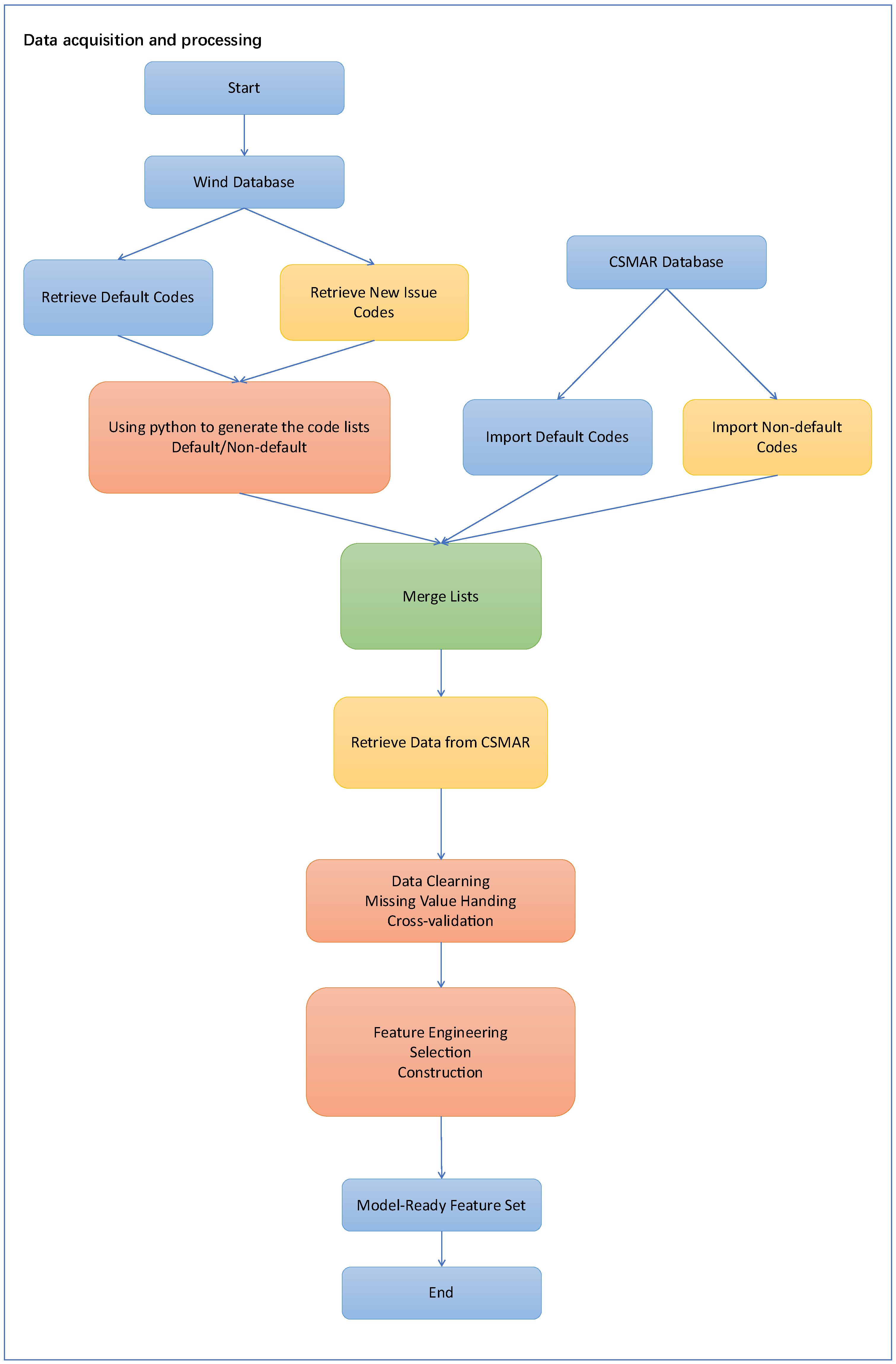
The empirical analysis is based on bond market data from two authoritative sources in China: Wind (WIND) financial terminal and China Stock Market & Accounting Research Database (CSMAR). The sample construction followed a rigorous five-step workflow to ensure accuracy and exclusivity between defaulted and non-defaulted bonds (summarized in Figure 1).

• Initial Identification: Bond codes for all recorded defaults were extracted from Wind’s default module, while a separate list of all newly issued bonds within the observation period was obtained from Wind’s issuance database.
• Sample Segregation: Using a Python 3.9.13 script, two mutually exclusive groups were created: (i) Defaulted Bonds and (ii) Non-Defaulted Bonds (all issued bonds minus the defaulted ones).
• Data Retrieval: Detailed bond-specific information for both groups was retrieved from the CSMAR database.
• Data Cleaning: Records with missing key variables were removed. The default status from CSMAR was further cross-validated against Wind default records by matching bond and issuer names to resolve discrepancies.
• Final Dataset: The cleaned data were merged into a unified dataset containing 522 defaulted bonds and 9918 non-defaulted bonds, resulting in a pronounced class imbalance with a default rate of approximately 5%. The dataset comprises 19 predictor variables and one binary outcome (default = 1). A detailed description of all features is provided in the Appendix A.

3.2. Feature Selection and Dimensionality Reduction

Assessing variable importance is a critical step, as a feature’s relevance often depends on its interactions with other predictors rather than its isolated effect [36,37]. To identify the most discriminative features for default prediction while ensuring robustness, this study employs a supervised, two-stage selection process that explicitly accounts for class imbalance and mitigates overfitting concerns. The process is conducted solely within the training data folds to prevent information leakage. The Random Forest (RF) algorithm was selected as the core feature importance evaluator for two primary reasons. First, RF naturally models non-linear relationships and complex interactions between features, which are prevalent in financial data, offering a more realistic assessment than linear filter methods (e.g., correlation-based selection) or unsupervised dimensionality reduction techniques (e.g., PCA). Second, RF provides a robust, data-driven importance score (e.g., mean decrease in Gini impurity) that is widely adopted for supervised feature selection [38,39,40]. Unlike unsupervised methods, which ignore the target variable, this supervised approach directly identifies features predictive of the specific outcome (default).

The selection process was executed in three consecutive stages:

Stage 1: Baseline Importance Assessment on Imbalanced Data

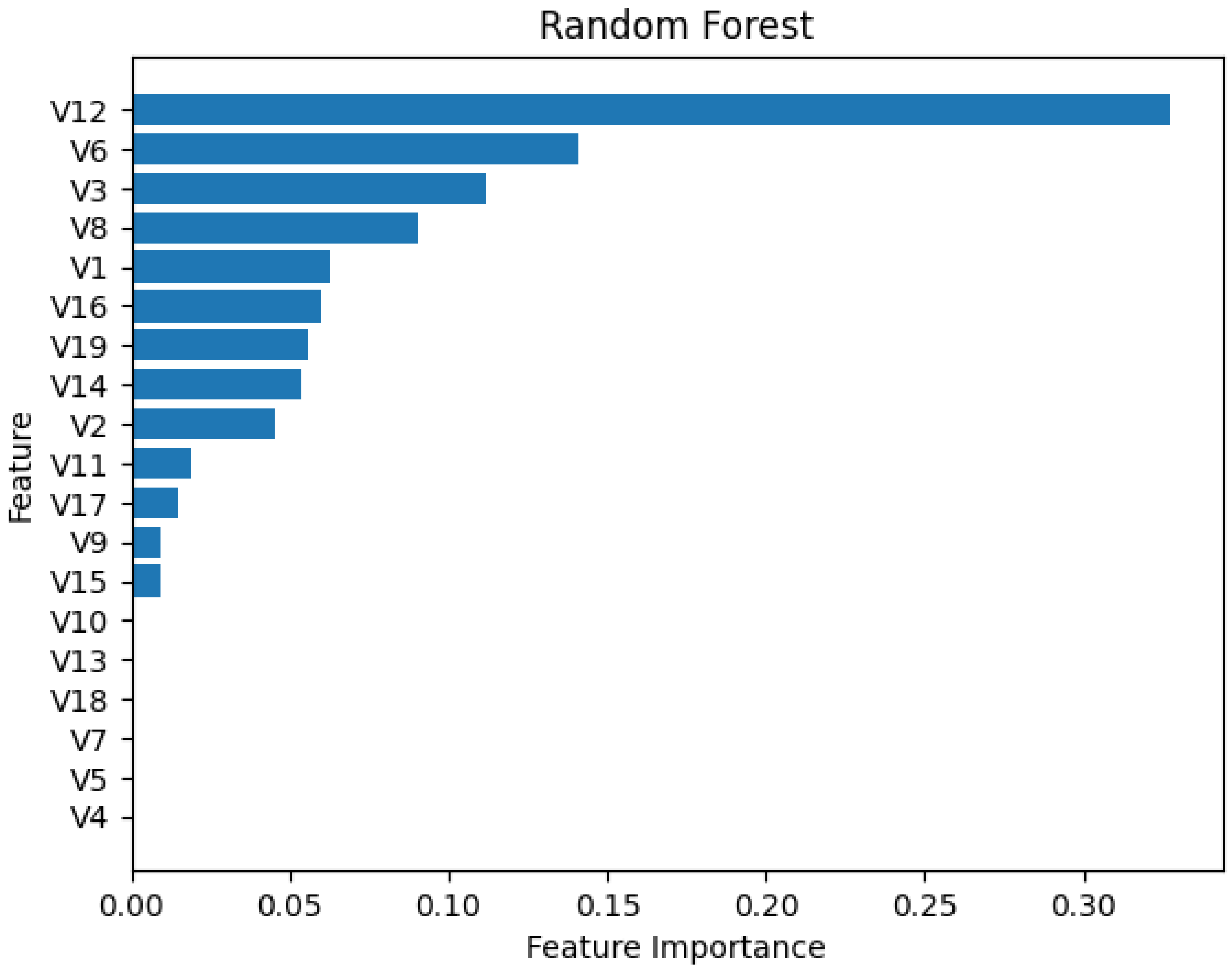
An initial RF model (configured with 1000 trees for stability) was trained on the original, imbalanced training set. The resulting feature importance ranking (Figure 2) served as a baseline, reflecting the variable relevance under the natural, skewed class distribution.

Stage 2: Importance Assessment Adjusted for Class Imbalance

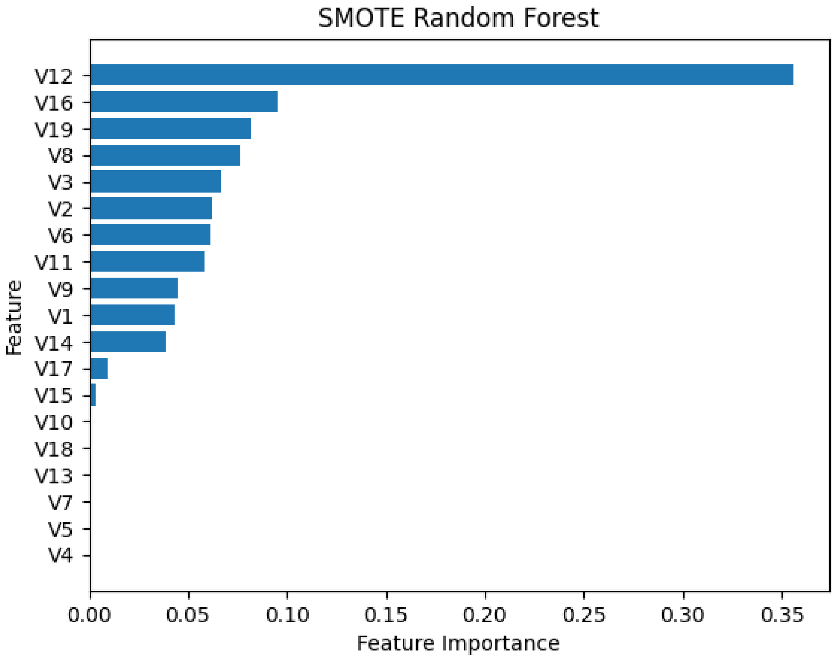
To address potential bias introduced by the severe class imbalance (5% default rate) and to directly mitigate concerns regarding the stability of the importance ranking, we repeated the analysis on a balanced dataset. Specifically, the Synthetic Minority Over-sampling Technique (SMOTE) was applied exclusively within the training folds of a cross-validation loop to generate balanced data. A new RF model was then trained on this balanced data to recompute feature importance (Figure 3). This two-stage approach allows us to distinguish features whose importance is robust across different data distributions from those that may be artifacts of the imbalance.

Stage 3: Conservative Feature Elimination and Overfitting Mitigation

A comparative analysis of the rankings from Stage 1 and 2 revealed notable shifts for some variables, confirming that class imbalance affects the assessment. To build a parsimonious and generalizable model, we adopted a conservative elimination rule: only features that consistently ranked in the lowest tier of importance across both the imbalanced and balanced analyses were considered redundant and removed. This resulted in the removal of six features (V4, V5, V7, V10, V13, V18). This stringent, consensus-based criterion reduces the risk of discarding informative features due to the peculiarities of a single analysis (e.g., imbalance bias) and thus helps mitigate overfitting at the feature selection stage. The final, reduced feature set was then used to train all subsequent models in the ensemble framework, which itself provides further regularization against overfitting.

3.3. Resampling Algorithms

Class imbalance, where the minority class (e.g., bond defaults) is significantly outnumbered by the majority class (non-defaults), poses a fundamental challenge to standard classifiers. Such models often exhibit a bias towards the majority class, leading to high overall accuracy but poor detection of the critical minority events. To mitigate this bias at the data level, resampling techniques are commonly employed to adjust the class distribution prior to or during model training. This study investigates and integrates two fundamental resampling strategies within the ensemble framework: the Synthetic Minority Over-sampling Technique (SMOTE) and Random Under-Sampling (RUS).

SMOTE [15] addresses the key limitation of simple random oversampling—the risk of overfitting caused by exact replication of minority samples. Instead, it generates synthetic samples for the minority class within the feature space. For a given minority instance $x_i$, SMOTE identifies its $k$-nearest neighbors belonging to the same class (typically $k=5$). A synthetic sample $x_{\mathrm{new}}$ is then created along the line segment connecting $x_i$ and a randomly chosen neighbor $x_{zi}$ via linear interpolation:

$$x_{\mathrm{new}}=x_i+\lambda \cdot (x_{zi}-x_i)$$

where $\lambda$ is a random number uniformly distributed in the interval [0, 1]. This approach effectively expands the decision region for the minority class, encouraging the learning of more generalizable boundaries and alleviating over-fitting.

In contrast to SMOTE, RUS is a simple under-sampling strategy that aims to balance the class distribution by randomly removing instances from the majority class until a desired balance ratio is achieved. While computationally efficient and straightforward, RUS carries the significant risk of discarding potentially informative data, which may lead to the loss of crucial patterns and a consequent degradation of model performance, especially in contexts where data from the majority class is also valuable for defining the decision boundary.

The selection of the classic SMOTE algorithm, among various advanced oversampling variants (e.g., ADASYN, Borderline-SMOTE), is based on two principal considerations that align with the core objective of this study. First, classic SMOTE serves as a stable and interpretable benchmark. Its linear interpolation mechanism is straightforward, which reduces the risk of introducing complex, hard-to-interpret synthetic samples that could obscure the causal relationships within financial data. This stability is crucial when the method is to be integrated into a complex, multi-layered ensemble framework. Second, and more importantly, the primary innovation of this work lies not in advancing the frontier of resampling algorithms per se, but in proposing a novel ensemble architecture capable of significantly amplifying the effectiveness of a well-established balancing technique. By demonstrating that a sophisticated integration of classic SMOTE within our DELC framework yields superior performance, we highlight the substantial gains achievable through architectural innovation, thereby offering a clear and focused contribution.

Given the complementary strengths and weaknesses of SMOTE (which creates information but may introduce noise) and RUS (which is simple but may discard information), an empirical pre-training analysis (detailed in Section 4.2) is conducted to determine the most effective resampling strategy for integration into the proposed double-ensemble architecture. A detailed mathematical formulation and algorithmic description of SMOTE and RUS are provided in the Appendix A. This data-driven approach ensures that the final model design is grounded in empirical performance rather than arbitrary selection.

3.4. Model Evaluation Metrics: Rationale and Computation

Given the high-stakes nature of default prediction and the severe cost associated with both false negatives (missing a true default) and false positives (unnecessary alarm), employing metrics that holistically evaluate performance across both classes is essential. Standard accuracy is misleading in cases of severe class imbalance, as a model that simply predicts the majority class (non-default) can achieve a deceptively high score. Therefore, we prioritize a suite of complementary metrics, with the Geometric Mean (G-mean) serving as our primary comprehensive measure.

All performance metrics are derived from the confusion matrix for the binary classification task, where default is designated as the positive class and non-default as the negative class. True positives (TP) and true negatives (TN) represent correctly predicted defaults and non-defaults, respectively, while false positives (FP) and false negatives (FN) denote the two types of errors: non-defaults incorrectly flagged as defaults (Type I error) and defaults missed by the model (Type II error).

From these four fundamental quantities, we compute a suite of complementary metrics. Sensitivity, also known as recall, measures the model’s ability to detect actual defaults and is given by TP/(TP + FN). Specificity, defined as TN/(TN + FP), captures the accuracy in identifying solvent firms. Precision, or TP/(TP + FP), reflects the reliability of a default warning. Overall accuracy, calculated as (TP + TN)/(TP + TN + FP + FN), provides a global measure of correctness but can be misleading under class imbalance. To balance precision and recall, the F1-score is computed as the harmonic mean of the two: 2 × (Precision × Recall)/(Precision + Recall).

Building on these, we employ Cohen’s Kappa (κ) to assess the agreement between model predictions and true labels while accounting for the agreement expected by chance. Kappa is calculated as

$$\kappa ={\displaystyle \frac{p_o-p_e}{1-p_e}}$$

where $p_o$ represents the observed agreement (accuracy) and $p_e$ denotes the probability of chance agreement. A value greater than zero indicates performance superior to random guessing, making it a more robust measure than raw accuracy for imbalanced settings.

Most importantly, our primary evaluation metric is the Geometric Mean (G-mean), defined as the square root of the product of Sensitivity and Specificity:

$$\mathrm{G}-\mathrm{mean}=\sqrt{\mathrm{Sensitivity}\times \mathrm{Specificity}}.$$

The G-mean is particularly suited for imbalanced classification because it penalizes models that perform well on only one class. A high G-mean can only be achieved when both the ability to detect defaults (Sensitivity) and the ability to avoid false alarms (Specificity) are concurrently high. This property makes it a robust and informative single metric for assessing model performance in the context of financial risk prediction, where both types of errors carry significant cost [41]. This set of metrics offers a multifaceted view of predictive performance, with particular emphasis on G-mean for evaluating minority-class detection under severe imbalance.

3.5. The Proposed DELC-SMOTE Architecture

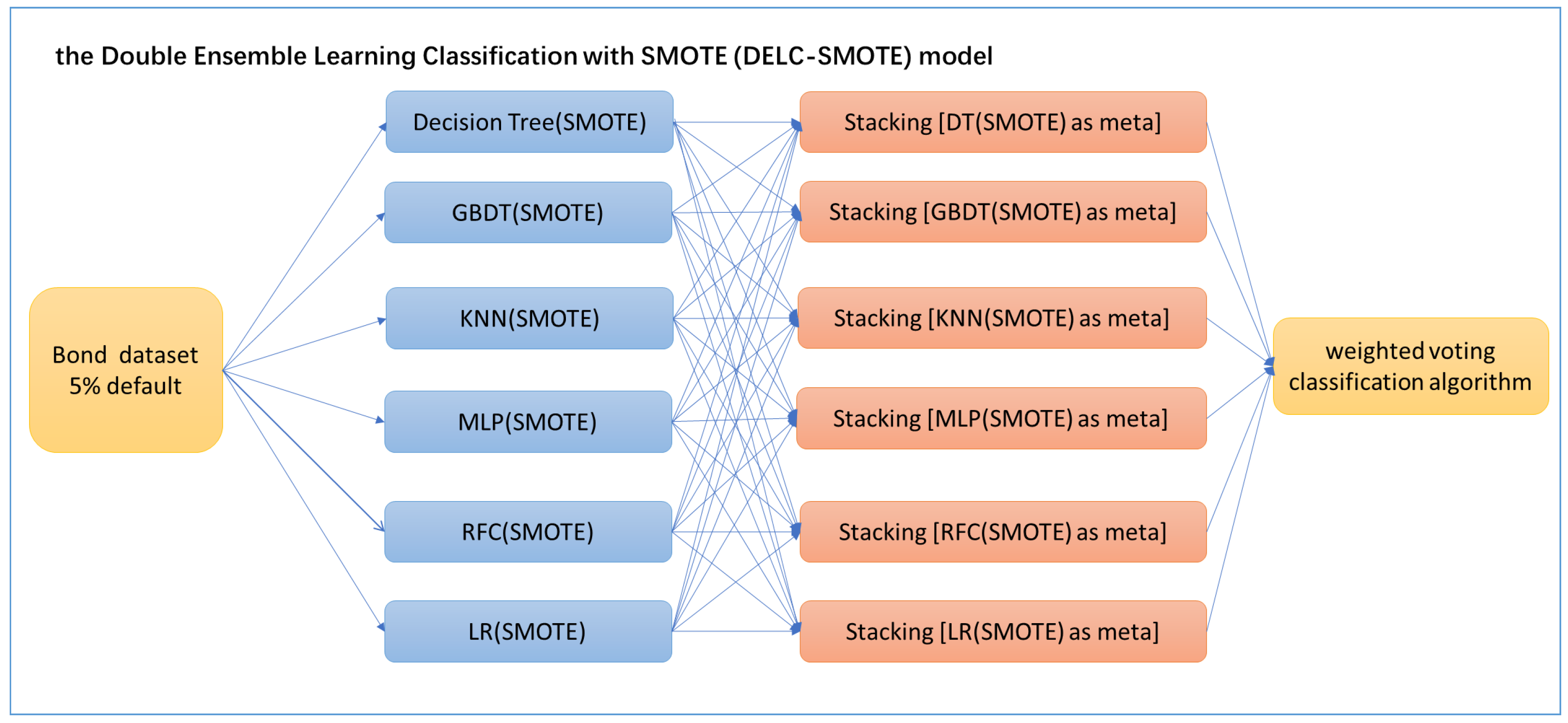
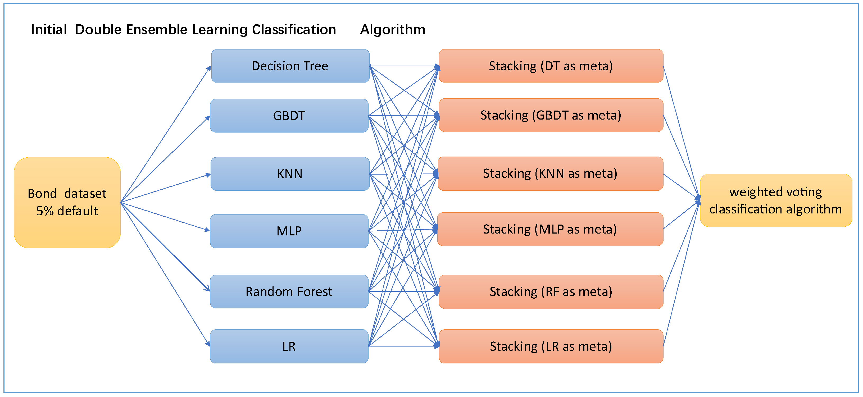
The core contribution is the Double-Ensemble Learning Classification with SMOTE (DELC-SMOTE) model, a novel two-phase hierarchical ensemble. Its architecture is illustrated in Figure 4.

Phase 1: Introspective Stacking for Algorithm-Specific Enhancement

In this phase, each of the six base learning algorithms—Decision Tree (DT), Gradient Boosting (GBDT), k-Nearest Neighbors (KNN), Multi-Layer Perceptron (MLP), Random Forest (RF), and Logistic Regression (LR)—undergoes a dedicated introspective Stacking procedure:

• Base Model Training: An initial model of algorithm A is trained on data balanced via SMOTE (applied within cross-validation folds).
• Homogeneous Meta-Learning: The predictions from this base model serve as new meta-features. A second model, also of type A, is trained on these features to refine the predictions. This step, denoted as Stacking (A as meta) in Figure 4, allows each algorithm family to self-correct, producing six specialized expert models. To generate unbiased meta-features for the introspective stacking phase, a 5-fold cross-validation procedure is employed within the training set. For each fold, the base model (trained on the other 4 folds after applying SMOTE) is used to predict the class probabilities for the samples in the held-out fold. These out-of-sample predictions are aggregated to form the meta-feature dataset for each base learner. A second model, also of type A, is then trained on these meta-features to refine the predictions. This step, denoted as Stacking (A as meta) in Figure 4, allows each algorithm family to self-correct, producing six specialized expert models.

Phase 2: Cross-Algorithm Fusion via Weighted Voting

Predictions from the six expert models are aggregated using Weighted Voting. The weight $w_i$ for the $i$-th expert is proportional to its G-mean performance on a held-out validation set: $w_i\propto {\mathrm{G}-\mathrm{mean}}_i$. The final prediction is determined by a weighted majority vote, effectively combining the diverse inductive biases of the different algorithm families.

3.5.1. DELC-SMOTE Training and Prediction Algorithms

The complete workflow is formalized in Algorithms 1 and 2.

Algorithm 1: DELC-SMOTE Training

Input: Imbalanced dataset ${\mathcal{D}}_{\mathrm{train}}$, base algorithms $\mathcal{A}$, SMOTE parameters $K,R$ Output: Expert models $\left\{E_t\right\}$, weights $\mathbf{w}$ 1: Split ${\mathcal{D}}_{\mathrm{train}}$ into ${\mathcal{D}}_{\mathrm{base}}$ (80%) and ${\mathcal{D}}_{\mathrm{val}}$ (20%) 2: for each algorithm $A_t\in \mathcal{A}$ do 3: // Step 1: Train base model with SMOTE using cross-validation for meta-features 4: Initialize an empty list $\mathrm{MetaFeatures}$ 5: Split ${\mathcal{D}}_{\mathrm{base}}$ into 5 folds $\{F_1,...,F_5\}$ 6: for $k=1$ to $5$ do 7:  ${\mathcal{D}}_{\mathrm{train}-\mathrm{fold}}\leftarrow {\mathcal{D}}_{\mathrm{base}}\setminus F_k$ 8:  ${\mathcal{D}}_{\mathrm{balanced}}\leftarrow \mathrm{SMOTE}\left({\mathcal{D}}_{\mathrm{train}-\mathrm{fold}},K,R\right)$ 9:  $M_t^{\left(k\right)}\leftarrow \mathrm{Train}(A_t,{\mathcal{D}}_{\mathrm{balanced}})$ 10:  ${\mathbf{P}}_k\leftarrow \mathrm{PredictProb}(M_t^{\left(k\right)},F_k)$ // Predict on held-out fold 11:  Append ${\mathbf{P}}_k$ to $\mathrm{MetaFeatures}$ 12: end for 13: ${\mathcal{D}}_{\mathrm{meta}}\leftarrow \mathrm{Assemble}\left(\mathrm{MetaFeatures}\right)$ // Out-of-sample predictions as features 14: // Step 2: Train introspective expert model on meta-features 15: $E_t\leftarrow \mathrm{Train}(A_t,{\mathcal{D}}_{\mathrm{meta}})$ 16: // Step 3: Evaluate expert model on validation set 17: $G_t\leftarrow \mathrm{G}-\mathrm{mean}\left(E_t\right({\mathcal{D}}_{\mathrm{val}}\left)\right)$ 18: end for 19: // Phase 2: Compute voting weights 20: for $t=1$ to $6$ do 21: $w_t\leftarrow G_t/\sum _{k=1}^6 G_k$ 22: end for 23: return $\left\{E_t\right\},\mathbf{w}$

Algorithm 2: DELC-SMOTE Prediction

Input: New instance $\mathbf{x}$, expert models $\left\{E_t\right\}$, weights $\mathbf{w}$ Output: Final prediction $\widehat{y}$ 1: for $t=1$ to $6$ do 2: ${\mathbf{s}}_t\leftarrow E_t\left(\mathbf{x}\right)$ // ${\mathbf{s}}_t=\left[s_t^{\left(0\right)},s_t^{\left(1\right)}\right]$ 3: end for 4: Initialize $V_0\leftarrow 0,V_1\leftarrow 0$ 5: for $t=1$ to $6$ do 6: $V_0\leftarrow V_0+w_t\cdot s_t^{\left(0\right)}$ 7: $V_1\leftarrow V_1+w_t\cdot s_t^{\left(1\right)}$ 8: end for 9: if $V_1>V_0$ then 10: $\widehat{y}\leftarrow 1$ 11: else 12: $\widehat{y}\leftarrow 0$ 13: end if 14: return $\widehat{y}$

3.5.2. Rationale for the Hierarchical, Introspective Design

The DELC-SMOTE architecture offers several distinct advantages that collectively contribute to its superior predictive performance. One key advantage lies in its specialized meta-learning approach: by employing homogeneous meta-learners—that is, using the same algorithm family for both base and meta-learning—the architecture aligns with each algorithm’s inherent error patterns, enabling more effective self-correction than would be possible with a generic meta-learner. This design choice allows each algorithm family to refine its predictions based on its own inductive biases, leading to more targeted improvements.

Furthermore, this hierarchical design ensures enhanced robustness through diversity at two complementary levels. Diversity is first established across the six heterogeneous algorithm types (Decision Tree, Random Forest, GBDT, KNN, MLP, and Logistic Regression), each capturing different aspects of the underlying data structure. It is then further amplified through the specialized refinement process, where each algorithm family develops its own optimized perspective on the balanced data. This multi-layered diversity maximizes generalization capacity and reduces the risk of overfitting.

Crucially, the architecture achieves effective imbalance mitigation by integrating SMOTE directly within each expert’s training loop rather than applying it as a global preprocessing step. This localized approach addresses class imbalance at the very source of learning for each individual model, strengthening each expert’s ability to detect minority-class defaults before their insights are fused in the weighted voting phase. By building robust specialized models first and then combining their strengths, the architecture systematically overcomes the limitations of both global resampling and homogeneous ensembles.

3.6. Benchmark Models for Ablation Study

To accurately evaluate the contribution of each design component within the proposed architecture and ensure a fair comparison, we constructed two benchmark models for ablation studies. It must be emphasized that the benchmark models—‘Initial DELC’ and ‘SMOTE Initial DELC’—employ the identical set of six base learners (Decision Tree, Gradient Boosting, K-Nearest Neighbors, Multi-Layer Perceptron, Random Forest, and Logistic Regression) and the identical two-tier ensemble architecture (introspective stacking + weighted voting) as the final DELC-SMOTE model. Their sole distinction lies in whether and how SMOTE resampling is integrated, thereby allowing us to isolate and quantify the impact of different design choices.

3.6.1. Initial DELC Model

This model retains the identical two-tier ensemble architecture of DELC-SMOTE but is trained directly on the original imbalanced data, without integrated SMOTE resampling (see Figure 5). It quantifies the performance gain attributable solely to the hierarchical ensemble design.

3.6.2. SMOTE Initial DELC Model

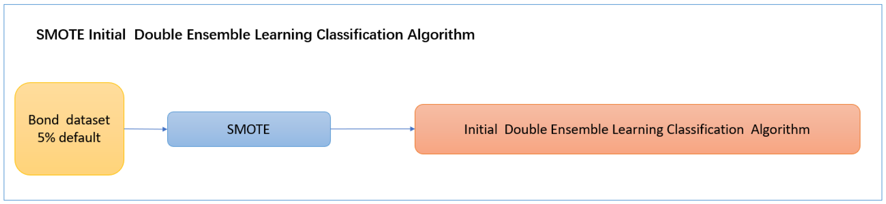
This model applies SMOTE globally once to balance the entire training dataset, which is then used to train the Initial DELC structure (see Figure 6). Comparing it with DELC-SMOTE highlights the advantage of local, integrated resampling within each expert’s training versus global preprocessing.

3.7. Robustness Testing Protocol

To systematically evaluate the model’s resilience to data imperfections, we designed and executed three distinct robustness tests. The following protocol details the specific procedures and parameters for each test, ensuring full transparency and reproducibility.

3.7.1. Noise Robustness Test

This test assesses the model’s sensitivity to low-level feature corruption or measurement errors. We corrupt the independent test set features by adding additive Gaussian white noise to each feature value. The noise for each feature is independently sampled from a normal distribution with a mean (μ) of 0 and a fixed standard deviation (σ) of 0.1, i.e., $ϵ\sim \mathcal{N}\left(\mathrm{0,0.01}\right)$. Formally, a corrupted feature vector $\tilde{X}$ is created from the original $X$ as $\tilde{X}=X+ϵ$, where ϵ is a vector of i.i.d. noise samples. The model’s performance (Accuracy) on this noisy test set is compared to its performance on the pristine test set to calculate the Noise Robustness score.

3.7.2. Constant Perturbation Robustness Test

This test evaluates the model’s stability against small, systematic shifts in the input data, simulating calibration drift or consistent measurement bias. We apply a constant perturbation of 0.1 to every feature value of every sample in the independent test set. The perturbed feature vector is calculated as $\tilde{X}=X+0.1$. The model’s performance on this uniformly shifted test set is then measured. The constant perturbation robustness score is the ratio of the model’s accuracy on the perturbed set to its accuracy on the original set.

3.7.3. Synthetic Outlier Robustness Test

This test probes the model’s vulnerability to extreme, anomalous samples in the test data by introducing artificially generated outliers. To generate these synthetic outliers, each feature value is independently sampled from a uniform distribution U(−5,5), creating feature vectors that lie well outside the typical range of the original data. Subsequently, we construct a mixed test dataset by sequentially replacing the top 10% of samples in the original test set, determined by integer division, with these synthetically generated outliers. The model’s performance is then evaluated on this adversarial dataset containing approximately 10% outliers. The Outlier Robustness score is defined as the ratio of the model’s accuracy on this mixed set to its accuracy on the original pristine test set, with higher scores indicating greater resilience to anomalous inputs.

3.8. Experimental Environment and Implementation Details

To ensure the reproducibility of our experiments, this section provides a comprehensive description of the technical environment, algorithm configurations, and implementation specifics. All experiments were conducted on a workstation equipped with an Intel Core i7-14700HX processor featuring 20 cores and 28 threads, operating at up to 5.5 GHz, alongside 192 GB of DDR5 RAM. The code was developed and executed under the Windows 11 operating system using Python 3.9.13 as the programming environment.

For data manipulation and computation, we employed pandas version 1.5.3 and numpy version 1.24.3. All machine learning algorithms, including base classifiers, ensemble components, and evaluation metrics, were implemented using scikit-learn version 1.3.0. The imbalanced-learn library (imblearn) version 0.11.0 was used for SMOTE and RUS implementations, while xgboost version 1.7.3 provided gradient boosting capabilities. Visualizations were generated using matplotlib version 3.7.1 and seaborn version 0.12.2.

To ensure reproducibility, a fixed random seed (random_state = 42) was set for all stochastic algorithms and data splitting procedures.

Table 1. Hyperparameter Configurations for Base Learners and Ensemble Components.

Algorithm	Library	Key Hyperparameters
Decision Tree (DT)	scikit-learn	random_state = 123
Gradient Boosting Decision Tree (GBDT)	scikit-learn	n_estimators = 1000, max_depth = 6, random_state = 1234
k-Nearest Neighbors (KNN)	scikit-learn	n_neighbors = 5
Multi-Layer Perceptron (MLP)	scikit-learn	hidden_layer_sizes = (500, 500), random_state = 123, early_stopping = True, validation_fraction = 0.25, max_iter = 10,000
Random Forest (RF)	scikit-learn	n_estimators = 1000, random_state = 42 (feature selection); n_estimators = 500, random_state = 42 (final ensemble base learner)
Logistic Regression (LR)	scikit-learn	C = 1 × 10−1
SMOTE	imblearn	random_state = 42
RUS	imblearn	Default parameters
Introspective Stacking	scikit-learn	cv = 5
Weighted Voting Ensemble	Custom	Weights: [0.6, 1.9, 5.0, 3.5, 2.5, 1.1]

summarizes the hyperparameter configurations for the six base learners and ensemble components.

The introspective stacking phase employed 5-fold cross-validation within the StackingClassifier to generate unbiased meta-features, while the weighted-voting meta-ensemble used soft voting with empirically optimized weights as detailed in Table 1. These configurations were maintained consistently throughout all experiments to ensure fair comparison across models.

4. Results

4.1. Performance of Base Learners on Imbalanced Data

To establish performance baselines, six individual base learners were evaluated using 5-fold cross-validation on the original imbalanced dataset. As presented in

Table 2. Performance of Base Learners (Trained on Imbalanced Data, 5-Fold CV Mean).

Classifiers	Geometric Mean	Sensitivity	Specificity	Precision	Accuracy
RF	0.8147 ± 0.0282	0.9915 ± 0.0020	0.6701 ± 0.0466	0.9824 ± 0.0024	0.9751 ± 0.0029
GBDT	0.8418 ± 0.0184	0.9866 ± 0.0033	0.7185 ± 0.0318	0.9849 ± 0.0017	0.9729 ± 0.0035
DT	0.7972 ± 0.0456	0.9782 ± 0.0025	0.6513 ± 0.0743	0.9812 ± 0.0039	0.9615 ± 0.0051
LR	0.6839 ± 0.0238	0.9867 ± 0.0028	0.4746 ± 0.0339	0.9722 ± 0.0018	0.9606 ± 0.0023
MLP	0.8080 ± 0.0611	0.9873 ± 0.0035	0.6645 ± 0.0979	0.9821 ± 0.0049	0.9709 ± 0.0029
KNN	0.7445 ± 0.0261	0.9901 ± 0.0016	0.5603 ± 0.0387	0.9767 ± 0.0020	0.9681 ± 0.0033

Note: Performance metrics are reported as mean ± standard deviation from 5-fold cross-validation.

, while all classifiers exhibited high sensitivity (>0.97), their specificity, the ability to correctly identify non-defaults, varied significantly. This trade-off underscores the inherent challenge of imbalanced learning: models can achieve high overall accuracy by predominantly predicting the majority class, but at the cost of failing to discriminate the critical minority class. Consequently, the Geometric Mean (G-mean), which balances sensitivity and specificity, provides a more informative assessment [41].

4.2. Pre-Training Analysis for Resampling Method Selection

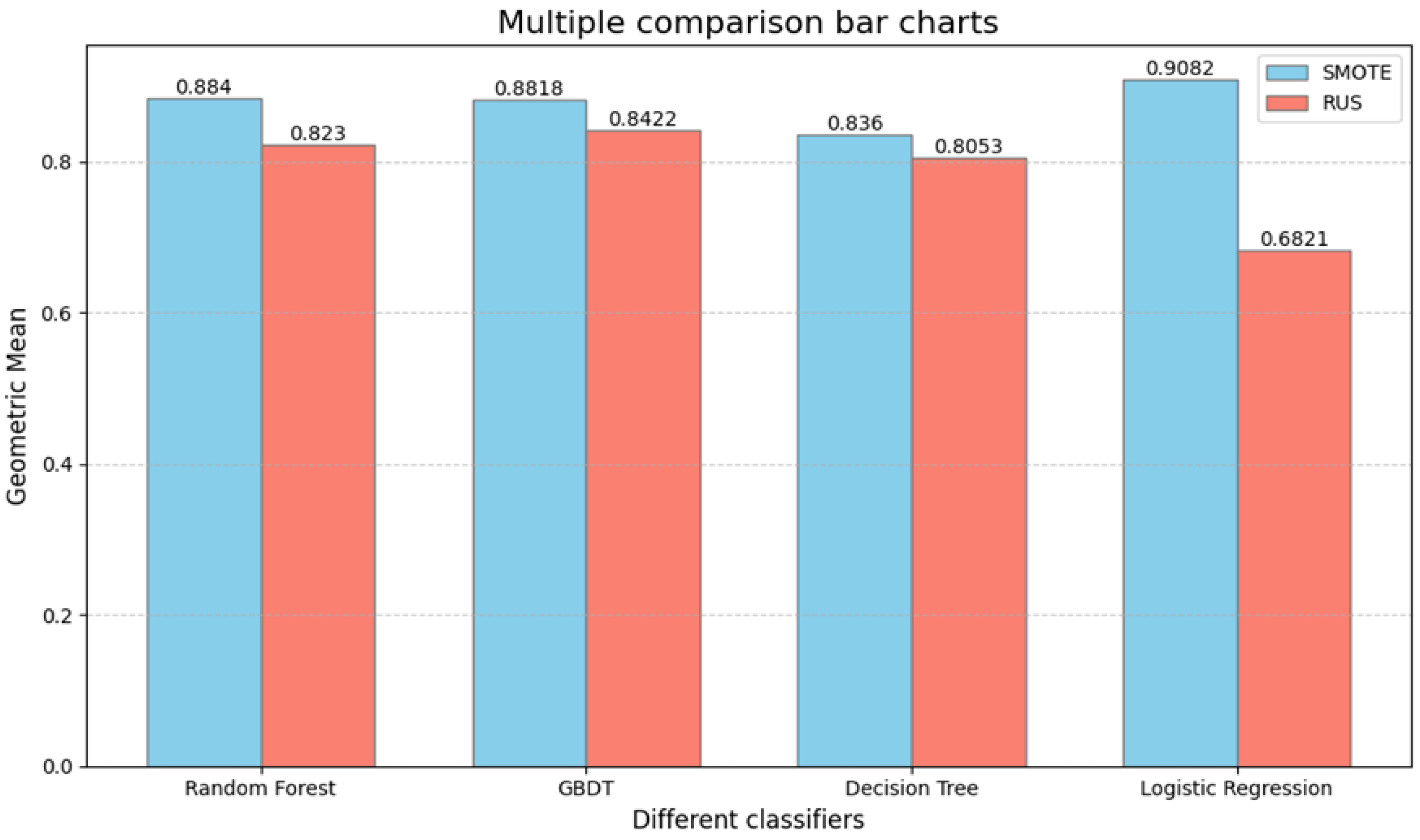
A pre-training experiment was conducted to empirically select the most appropriate resampling technique for integration into the ensemble framework. The six base learners were independently trained using 5-fold cross-validation, each combined with either SMOTE or RUS within the training folds. The mean performance metrics across folds are reported in

Table 3. Performance of Base Learners Integrated with SMOTE (5-Fold CV Mean).

Classifiers	Geometric Mean	Sensitivity	Specificity	Precision	Accuracy
RF (SMOTE)	0.8840 ± 0.0152	0.9817 ± 0.0024	0.7963 ± 0.0274	0.9890 ± 0.0015	0.9722 ± 0.0027
GBDT (SMOTE)	0.8818 ± 0.0170	0.9834 ± 0.0021	0.7909 ± 0.0320	0.9887 ± 0.0017	0.9736 ± 0.0013
DT (SMOTE)	0.8360 ± 0.0403	0.9748 ± 0.0051	0.7184 ± 0.0681	0.9847 ± 0.0036	0.9617 ± 0.0056
LR (SMOTE)	0.9082 ± 0.0198	0.9027 ± 0.0044	0.9142 ± 0.0410	0.9949 ± 0.0024	0.9033 ± 0.0041
MLP (SMOTE)	0.8901 ± 0.0253	0.9638 ± 0.0069	0.8228 ± 0.0508	0.9902 ± 0.0026	0.9566 ± 0.0047
KNN (SMOTE)	0.8907 ± 0.0063	0.9516 ± 0.0049	0.8338 ± 0.0155	0.9907 ± 0.0008	0.9455 ± 0.0040

(SMOTE) and

Table 4. Performance of Base Learners Integrated with RUS (5-Fold CV Mean).

Classifiers	Geometric Mean	Sensitivity	Specificity	Precision	Accuracy
RF (RUS)	0.8230 ± 0.0208	0.9915 ± 0.0024	0.6835 ± 0.0336	0.9831 ± 0.0017	0.9758 ± 0.0033
GBDT (RUS)	0.8422 ± 0.0150	0.9876 ± 0.0019	0.7184 ± 0.0261	0.9849 ± 0.0013	0.9739 ± 0.0019
DT (RUS)	0.8053 ± 0.0253	0.9802 ± 0.0035	0.6621 ± 0.0426	0.9818 ± 0.0022	0.9640 ± 0.0036
LR (RUS)	0.6821 ± 0.0219	0.9867 ± 0.0025	0.4719 ± 0.0305	0.9720 ± 0.0016	0.9605 ± 0.0027
MLP(RUS)	N/A	N/A	N/A	N/A	N/A
KNN(RUS)	N/A	N/A	N/A	N/A	N/A

Note: MLP and KNN encountered compatibility issues with the RUS pipeline (N/A).

(RUS).

The comparative analysis, visualized in Figure 7 (G-mean), clearly indicated that SMOTE consistently yielded superior and more robust performance compared to RUS across all compatible base learners. The average G-mean improvement of SMOTE over RUS for the four common classifiers (RF, GBDT, DT, LR) was 12.02%. Furthermore, SMOTE maintained compatibility with all six diverse base learners, which is crucial for building a heterogeneous ensemble. Therefore, SMOTE was selected as the resampling method for integration into the proposed DELC-SMOTE model.

4.3. Performance of Benchmark (Ablation) Ensemble Models

The results of the two benchmark models, constructed to ablate components of the final design, are shown in

Table 5. Performance of Benchmark Ensemble Models (5-Fold CV Mean).

Classifiers	Geometric Mean	Sensitivity	Specificity	Precision	Accuracy
Initial DELC	0.8405 ± 0.0273	0.9879 ± 0.0023	0.7156 ± 0.0455	0.9848 ± 0.0023	0.9740 ± 0.0032
SMOTE Initial DELC	0.8415 ± 0.0182	0.9860 ± 0.0010	0.7185 ± 0.0309	0.9849 ± 0.0017	0.9724 ± 0.0014

. Both models employ the same six base learners and two-tier ensemble architecture as DELC-SMOTE. The differences in their results directly reflect the utility of distinct resampling integration strategies.

The Initial DELC, which employs our proposed double-ensemble architecture without integrated resampling, showed a marked improvement over the best single base learner. Applying SMOTE as a global preprocessing step (SMOTE Initial DELC) yielded further gains, demonstrating the necessity of addressing class imbalance. However, both benchmarks were ultimately outperformed by the fully integrated DELC-SMOTE model.

4.4. Performance and Generalizability of the Proposed DELC-SMOTE Model

4.4.1. Performance Under the Primary Experimental Setting

The proposed DELC-SMOTE model demonstrated superior performance under the primary experimental setting (5% default rate), as detailed in

Table 6. Performance of the Proposed DELC-SMOTE Model (Primary Setting: ~5% Imbalance).

Indicator Name	Value (Mean ± SD from 5-Fold CV)
Geometric Mean	0.9152 ± 0.0216
Sensitivity	0.9616 ± 0.0022
Specificity	0.8715 ± 0.0425
Precision	0.9929 ± 0.0024
Accuracy	0.9570 ± 0.0018
F1-Score	0.981138
Kappa	0.689177

. Most notably, it achieved a G-mean of 0.9152 and a specificity of 0.8715, representing substantial improvements over the best benchmark model (SMOTE Initial DELC). The model also maintained exceptionally high precision (0.9929) and a strong F1-Score (0.9811).

4.4.2. Sensitivity of Predictive Performance to Class Imbalance Ratio

To thoroughly evaluate the model’s generalizability, we extended the evaluation to scenarios with different class imbalance ratios (2%, 10%, and 20%). The results, presented in

Table 7. Predictive Performance of DELC-SMOTE Across Different Class Imbalance Ratios.

Imbalance Ratio (Default %)	Geometric Mean (G-Mean)	Specificity	Sensitivity (Recall)	Accuracy
2%	0.8589	0.7778	0.9485	0.9452
10%	0.9057	0.8652	0.9481	0.9406
20%	0.9542	0.9419	0.9666	0.9617

, reveal a clear trend: as the class distribution becomes more balanced (default rate increases), the model’s performance on the key balanced metrics, G-mean and Specificity, improves substantially. Even under the highly imbalanced 2% scenario, the model maintains a G-mean above 0.85 and a Specificity near 0.78, while retaining a very high Sensitivity (~0.95). This demonstrates that the core architecture of DELC-SMOTE does not collapse under severe class imbalance. It successfully mitigates the bias towards the majority class, preserving a strong ability to identify true defaults (high Sensitivity) while still achieving a reasonable ability to correctly identify non-defaults (moderate Specificity). While the absolute performance of DELC-SMOTE is positively correlated with the balance of the dataset, its architectural effectiveness is robust across a spectrum of imbalance ratios. The model provides meaningful, superior performance even at a 2% default rate, a common and challenging level of imbalance in real-world credit risk datasets. This suggests the model is a viable and robust choice across different market segments or economic periods that may exhibit different inherent default rates.

4.5. Robustness Evaluation

4.5.1. Robustness Testing Results Under Primary Setting

Following the detailed protocol established in Section 3.7, we quantitatively assessed the stability of the DELC-SMOTE model under adverse data conditions for the primary experimental setup (5% imbalance). The results are summarized in

Table 8. Robustness Testing Results of DELC-SMOTE (Primary Setting).

Test Category	Test Protocol Summary	Robustness Score
Noise Robustness	Adding Gaussian noise $\mathcal{N}\left(\mathrm{0,0.01}\right)$ to all test features.	0.901
Constant Perturbation	Adding a constant shift of +0.1 to all test feature values.	0.875
Synthetic Outlier	Replacing 10% of test data with outliers from $\mathcal{U}(-\mathrm{5,5})$.	0.958

. The model demonstrated strong resilience, maintaining high performance across all scenarios. Specifically, it achieved a score of 0.901 in Noise Robustness testing, indicating its ability to withstand feature corruption and data quality issues. Under Constant Perturbation, it retained stable predictions with a score of 0.875, confirming that its decisions are not based on fragile or spurious patterns within the data. Most notably, the model exhibited exceptional Outlier Robustness with a score of 0.958, suggesting that its predictive logic is anchored to core, representative data relationships rather than being unduly influenced by extreme values.

4.5.2. Robustness Sensitivity to Class Imbalance

To comprehensively evaluate the model’s stability under diverse data conditions, the robustness tests were extended to datasets with different class imbalance ratios.

Table 9. Robustness of DELC-SMOTE Across Different Class Imbalance Ratios.

Imbalance Ratio (Default %)	Noise Robustness	Perturbation Robustness	Outlier Robustness
2%	0.7668	0.6530	0.9317
10%	0.8621	0.7810	0.9202
20%	0.9285	0.9310	0.9400

presents the Noise, Perturbation, and Outlier Robustness scores for the DELC-SMOTE model evaluated under three distinct imbalance scenarios (2%, 10%, and 20% default rates).

The extended analysis reveals a clear trend: the model demonstrates increasing robustness to noise and perturbations as the class distribution becomes more balanced (i.e., as the default rate increases from 2% to 20%). This suggests that the decision boundary learned from a more balanced dataset is inherently more stable and less sensitive to feature corruption or systematic shifts. In contrast, Outlier Robustness remains consistently high (all scores > 0.92) across all imbalance scenarios. This indicates that the model’s core predictions are strongly anchored to representative data patterns and are not easily misled by extreme anomalous samples, regardless of the underlying class imbalance level.

Collectively, the results from Section 4.5.1 and Section 4.5.2 affirm that the DELC-SMOTE model is not only accurate but also reliable and stable. Its performance remains consistent even when faced with imperfect, noisy, or anomalous data. The sensitivity analysis further reveals that while the model’s robustness to certain perturbations correlates with class balance, its exceptional and consistent resilience to outliers is a key strength. This combination of traits fulfills a critical requirement for practical risk management systems that must operate reliably under diverse and uncertain data conditions. The high outlier robustness across all imbalance scenarios is particularly significant, as it suggests the model’s decision-making is based on fundamental, representative relationships within the data rather than being skewed by rare, extreme cases.

4.6. Performance Comparison and Visualization

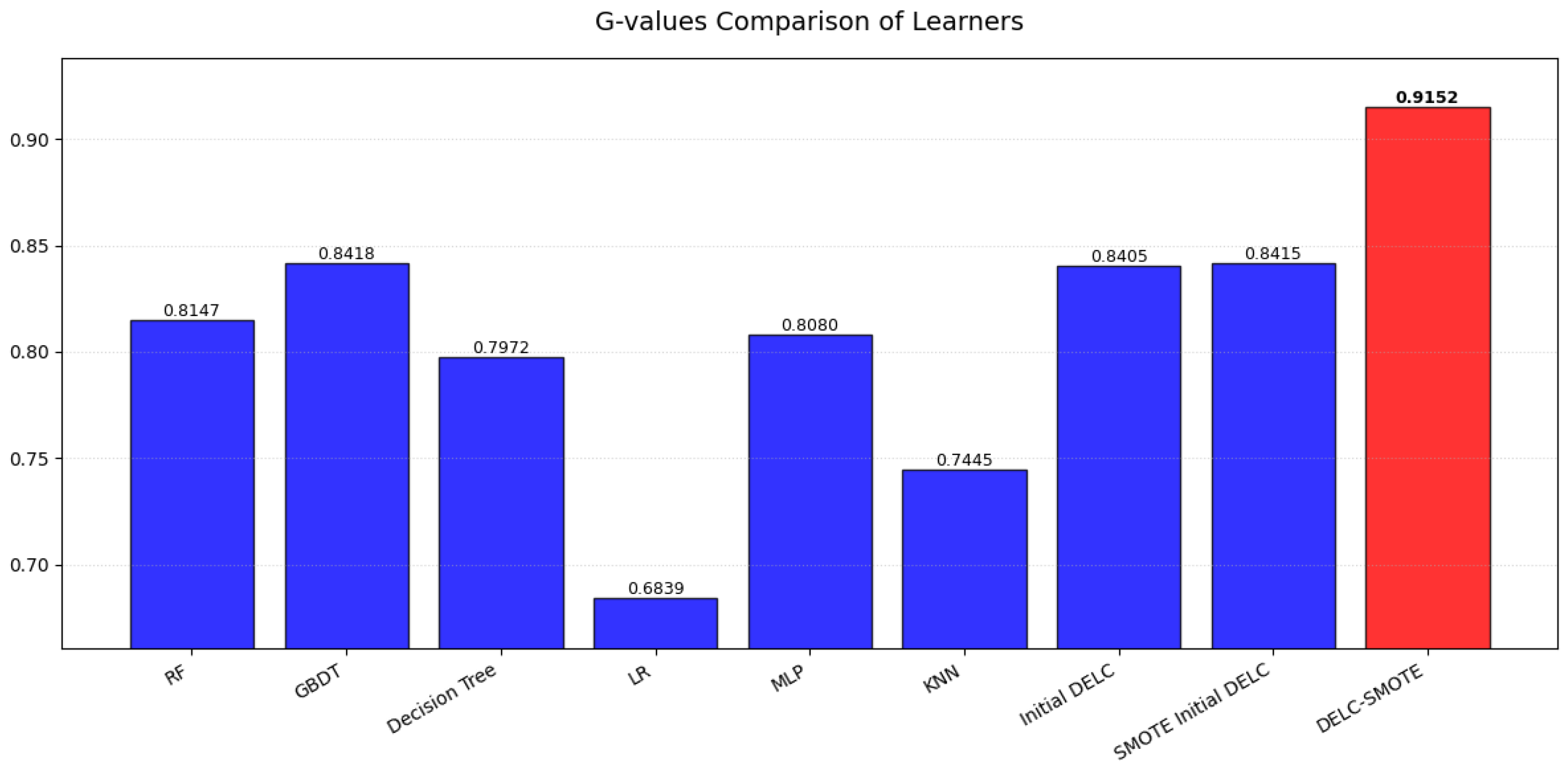
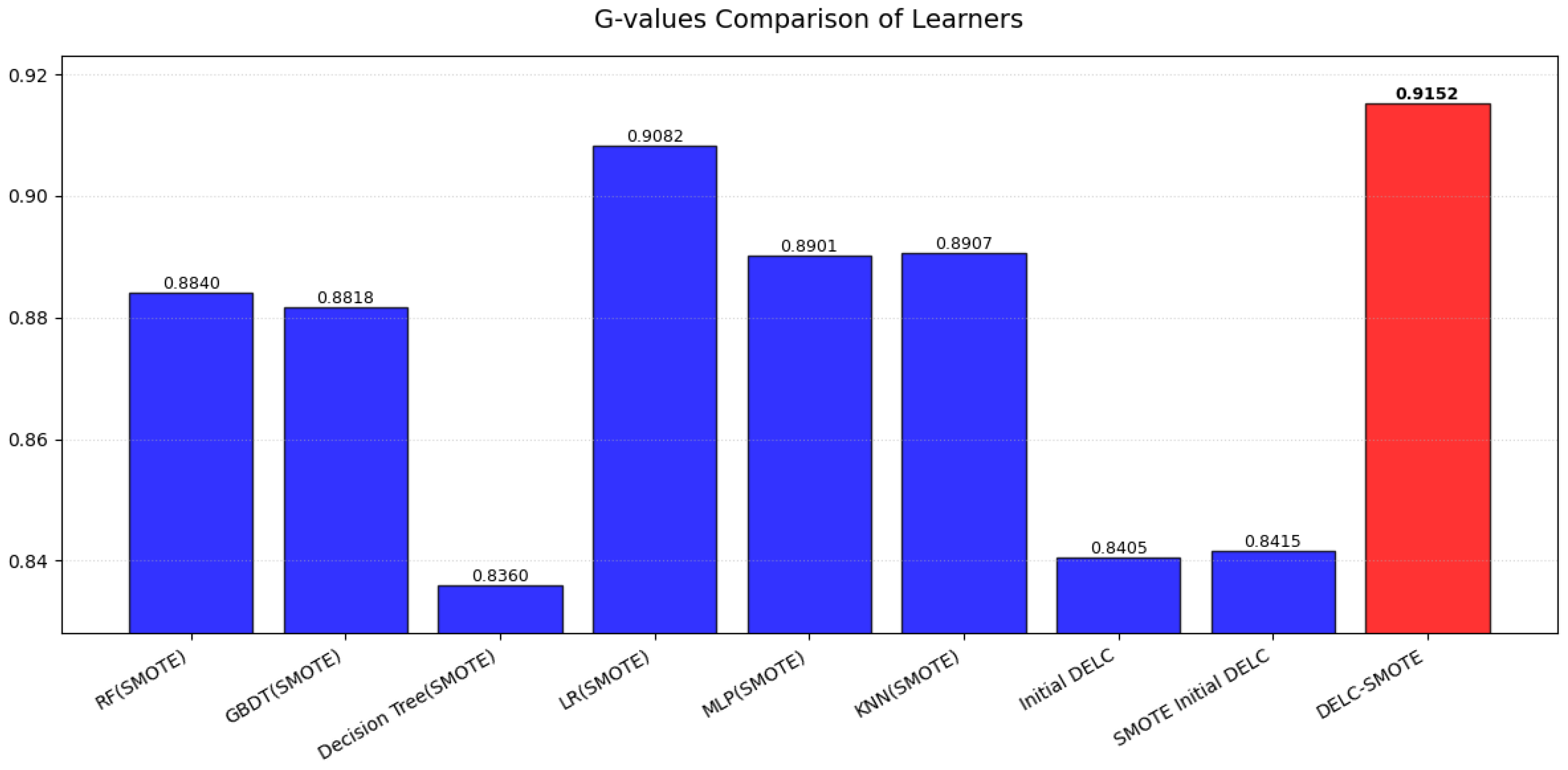
The superior performance of the proposed DELC-SMOTE model is clearly demonstrated through visual comparison. As shown in Figure 8, which compares the Geometric Mean (G-mean) of all base learners trained on the original imbalanced data and the benchmark ensemble models, DELC-SMOTE substantially outperforms all other models. For instance, while individual base learners such as RF, GBDT, and MLP achieve G-mean values ranging from 0.6839 to 0.8418, and the benchmark ensemble models (Initial DELC and SMOTE Initial DELC) attain 0.8405 and 0.8415, respectively, the DELC-SMOTE model reaches a significantly higher G-mean of 0.9152. This visual evidence underscores that the hierarchical ensemble framework successfully synthesizes and surpasses the strengths of its individual components.

A focused comparison against the SMOTE-enhanced base learners (from Table 3) further illustrates this point. Figure 9 shows that while individual models like KNN (SMOTE) and LR (SMOTE) achieve strong G-mean scores of 0.8907 and 0.9082, respectively, the DELC-SMOTE model attains the highest value of 0.9152, confirming its ability to extract synergistic predictive power through sophisticated model fusion rather than relying on any single enhanced learner.

4.7. Statistical Significance Tests and Model Stability Evaluation

This section presents an in-depth analysis of statistical significance and stability for the proposed DELC-SMOTE model. All analyses in this section are based on the model’s performance on a held-out independent test set (n = 3132), complementing the final performance metrics reported in Section 4.4.

This study employs a phased evaluation strategy. Results from model development, comparison, and selection in Section 4.2, Section 4.3 and Section 4.4 are based on 5-fold cross-validation. Upon finalizing the DELC-SMOTE architecture, a final evaluation was conducted on a preserved independent test set (30% of the total data), which serves as the basis for all subsequent statistical significance tests. It is important to note the difference between the accuracy obtained in the independent test (0.8116) and the average accuracy from 5-fold cross-validation (~0.9646). This phenomenon is recognized in imbalanced learning: cross-validation can yield a deceptively high average accuracy when class imbalance is severe, as models may lean towards predicting the majority class. The independent test set provides a stricter, less biased estimate of the model’s generalization ability. The reported accuracy (0.8116), when considered alongside the balanced metrics, provides a more realistic reflection of the model’s practical efficacy in risk-warning scenarios. Key statistics from this evaluation are summarized in

Table 10. Summary of Statistical Evaluation for DELC-SMOTE on the Independent Test Set.

Evaluation Dimension	Metric/Test	Result	Statistical Implication and Interpretation
Point Estimate	Test Set Accuracy	0.8116	Final model performance on unseen, independent data.
Interval Estimate	Accuracy 95% CI (Bootstrap)	[0.7987, 0.8254]	Stable performance range validated via resampling.
Dispersion & Stability	Bootstrap Accuracy Std. Dev.	0.0075	Extremely low performance volatility; the model is highly stable.
Model Comparison Test	McNemar’s Test (vs. Key Benchmark)	χ2 = 392.70, p < 0.001	Predictions are systematically and highly significantly different.
Generalization Test	Wilcoxon Signed-Rank Test (Train vs. Test Acc.)	p = 0.0637	The difference in distribution is marginally significant; no evidence of over-fitting.

.

4.8. Feature Importance Analysis

Having established the predictive performance of DELC-SMOTE in Section 4.1, Section 4.2, Section 4.3, Section 4.4 and Section 4.5, we now examine the internal drivers of these predictions through feature importance analysis. To enhance interpretability and identify the key drivers of default risk captured by our model, we analyzed global feature importance using the Random Forest algorithm trained on the SMOTE-balanced dataset (as described in Section 3.2). Figure 3 presents the complete feature importance ranking based on the mean decrease in Gini impurity, while

Table 11. Top Five Features Influencing Default Prediction: Importance Scores and Economic Intuition.

Rank	Feature (Code) and Name	Importance Score	Economic and Financial Intuition
1	V12: Coupon Rate	0.325	Represents the annual interest rate paid to investors. For fixed-rate bonds, it embodies the risk premium demanded at issuance, reflecting market-perceived credit risk.
2	V16: Resale Capability	0.280	Binary indicator of whether the bond can be sold back to the issuer before maturity. This put option provides investors with downside protection, potentially signaling lower default risk.
3	V19: Day Count Basis	0.240	Categorical variable indicating the interest calculation convention (ACT/ACT or A/365). May proxy for bond type or market segment differences.
4	V8: Bond Maturity	0.220	Measured in years from issuance to full repayment. Longer maturity exposes investors to greater uncertainty regarding future cash flows, interest rate fluctuations, and refinancing risks.
5	V3: Bond Type	0.180	Categorical variable distinguishing interest-bearing bonds from other types. Incorporates structural, regulatory, and legal dimensions of risk across different bond categories.

summarizes the top five most influential features along with their importance scores and economic interpretations.

5. Discussion

5.1. Interpretation of DELC-SMOTE Superiority and Practical Implications

The results presented in Section 4 demonstrate that the DELC-SMOTE model achieves a G-mean of 0.9152 and a specificity of 0.8715 (Table 6), representing substantial improvements over the best benchmark model (Initial DELC: 0.8405; SMOTE Initial DELC: 0.8415). The magnitude of this improvement (approximately 9% in G-mean) raises an important question of why the hierarchical integration of SMOTE yields such gains when global preprocessing does not. The answer, we argue, lies in the alignment between the architecture and the nature of imbalanced financial data. Global resampling creates a single synthetic landscape that may not equally suit all algorithms, whereas introspective stacking allows each learner to develop expertise on a data representation tailored to its own inductive biases.

This interpretation is supported by three lines of empirical evidence. First, the 12.02% average G-mean improvement of SMOTE over RUS across common classifiers (Section 4.2) confirms that algorithm-specific responses to resampling vary substantially. Second, the McNemar’s test result (p < 0.001, Table 10) establishes that DELC-SMOTE’s predictions are systematically different from the benchmark’s, not merely a marginal improvement. Third, the close alignment between training and test performance (Wilcoxon p = 0.0637, test accuracy 0.8116 vs. training 0.7990) indicates that this specialized learning does not come at the cost of overfitting. Together, these findings suggest that the value of the DELC-SMOTE architecture lies not in any single component, but in the synergy between differentiated resampling, algorithm-specific refinement, and ensemble fusion.

The model’s exceptionally high precision (0.9929) and specificity (0.8715) carry important practical implications. In risk management, false positives, flagging solvent firms as defaults, incur tangible costs: unnecessary reviews, customer relationship strain, and operational inefficiency. A precision of 0.9929 means that fewer than 1 in 100 default warnings are false alarms, substantially reducing these burdens. The moderate Cohen’s Kappa (0.6892) also suggests that the model’s agreement with true labels substantially exceeds chance.

5.2. Robustness and Performance Under Varying Imbalance Ratios

The sensitivity analysis in Section 4.4.2 reveals a monotonic relationship between class balance and model performance: as the default rate increases from 2% to 20%, G-mean rises from 0.8589 to 0.9542, and specificity from 0.7778 to 0.9419 (Table 7). This pattern, while intuitive, merits deeper examination. The 21.1% relative improvement in specificity substantially exceeds the 11.1% improvement in G-mean, suggesting that the model’s ability to avoid false positives is disproportionately sensitive to minority class representation. This asymmetry may reflect the weighted voting mechanism’s design: with more positive (non-default) examples, the ensemble can more confidently overrule false positive predictions from individual experts.

From a theoretical standpoint, these results align with Krawczyk’s [24] observation that decision boundary precision improves with minority class density. However, the graceful degradation under an extreme 2% imbalance (G-mean 0.8589) is noteworthy. It suggests that DELC-SMOTE’s hierarchical structure provides a form of built-in regularization that prevents the complete collapse common in single classifiers trained on severely imbalanced data (Brown & Mues, [21]). From a practical standpoint, this result is encouraging. It suggests that while DELC-SMOTE is optimized for a ~5% default rate, its performance degrades gracefully and predictably under even more severe imbalance. This characteristic is vital for real-world applications where the base rate of default can shift unexpectedly over economic cycles, for instance, during financial crises when default rates may spike. The model’s ability to maintain robust performance across a spectrum of imbalance ratios enhances its practical utility and trustworthiness.

The robustness tests in Section 4.5 further illuminate the model’s stability characteristics. The consistently high outlier robustness (>0.92 across all imbalance scenarios in Table 9) indicates that extreme anomalous values do not disproportionately influence predictions, a property consistent with the ensemble’s averaging of diverse experts. In contrast, the progressive improvement in noise and perturbation robustness with increasing class balance (from 0.7668 to 0.9285 for noise; from 0.6530 to 0.9310 for perturbation) suggests that a richer minority class representation helps the model learn more stable decision boundaries that are less sensitive to feature-level corruption.

5.2.1. Robustness and Generalization as Key Advantages

The double-ensemble framework’s robustness can be understood through the lens of ensemble diversity. By fusing predictions from six heterogeneous and introspectively refined experts, the architecture effectively averages out the idiosyncratic errors that any single model might make on corrupted or anomalous data. This interpretation is consistent with Zhou’s [12] “many could be better than all” principle, which posits that a diverse ensemble can outperform any single model by compensating for individual weaknesses. The robustness scores (0.901 under noise, 0.875 under perturbation, and 0.958 under outliers, see Table 8) provide empirical quantification of this theoretical advantage.

The bootstrap analysis (Section 4.7) offers additional insight into the model’s stability. The extremely low standard deviation of 0.0075 for accuracy estimates indicates that DELC-SMOTE’s performance is remarkably insensitive to the specific composition of the training and test splits. This property is particularly valuable for practical deployment, where models must perform reliably across different time periods and market conditions. It also enhances the scientific credibility of our findings by demonstrating that reported performance is not an artifact of favorable data partitioning.

5.2.2. An Unexpected Finding: The Sensitivity-Specificity Trade-Off

Despite its overall superior performance, a closer examination of the results reveals an intriguing pattern. While DELC-SMOTE achieves a substantial gain in specificity (0.8715) compared to the SMOTE Initial DELC benchmark (0.7185), its sensitivity (0.9616) is marginally lower than that of the benchmark (0.9860). This trade-off invites several interpretations. One possibility is that the weighted voting mechanism, optimized on G-mean, inherently prioritizes balance over maximizing any single metric. Another is that the introspective stacking phase, by refining each expert’s predictions, may inadvertently dampen the most extreme (and potentially correct) default signals in favor of consensus. The moderate Cohen’s Kappa (0.6892) supports this interpretation: the model achieves strong but not perfect agreement, suggesting that the ensemble’s conservatism trades some sensitivity for higher precision and specificity. Practically, it highlights an inherent tension in risk modeling: the choice between catching more defaults (sensitivity) and minimizing false alarms (specificity) depends on the relative costs of each error type. DELC-SMOTE’s current configuration favors specificity, and it is a defensible choice given the high operational costs of false positives.

5.3. Interpretability and Economic Implications

The feature importance analysis presented in Section 4.8 (Table 11) reveals several meaningful patterns that merit discussion. Perhaps surprisingly, coupon rate (V12) emerges as the dominant predictor of default risk, with an importance score (0.325) substantially higher than any other feature. This finding invites careful interpretation. At first glance, one might expect credit rating to dominate, as it did in many prior studies [27]. However, the prominence of the coupon rate may reflect a fundamental characteristic of the Chinese bond market during the sample period. For fixed-rate bonds, which constitute the majority of the sample, the coupon rate directly embodies the market’s assessment of default risk at the time of issuance. Higher perceived risk translates into higher required yields. The fact that this market-based signal outperforms even credit ratings suggests that in the Chinese context, the pricing mechanism may incorporate information not fully captured by rating agencies, a phenomenon consistent with findings by Lu and Zhuo [3], who noted that Chinese credit ratings have historically exhibited limited variation and may lag market signals.

The second-ranked feature, resale capability (V16), carries an importance score of 0.280, underscoring the significance of embedded options in bond valuation. Bonds with resale options allow investors to sell the bond back to the issuer under specified conditions, effectively providing downside protection. The model’s heavy reliance on this feature suggests that such contractual protections are strongly predictive of lower default risk. This may be either because they attract more sophisticated investors, discipline issuer behavior, or both. This finding aligns with research by Hu et al. [4] on the intra-industry spillover effects of default, which highlighted the importance of bond-specific contractual features in transmitting risk signals.

The day count basis (V19), appearing as the third most important feature (0.240), is more unexpected. This variable captures the convention for calculating accrued interest. One possible interpretation is that it proxies for bond type or market segment in ways not fully captured by the bond type variable (V3). For instance, certain bond categories may systematically use one day-count convention, making V19 a surrogate for unobserved structural differences. Alternatively, it could reflect differences in market practice that correlate with issuer characteristics or bond complexity. This finding suggests an avenue for future research: a more granular investigation of how apparently technical bond features may encode meaningful risk information.

Bond maturity (V8) and bond type (V3) rank fourth and fifth, with scores of 0.220 and 0.180, respectively. The inclusion of maturity among top predictors is consistent with theoretical expectations: longer maturities expose investors to greater uncertainty over extended time horizons, including potential changes in the issuer’s financial condition and macroeconomic shocks [22]. The prominence of bond type reinforces the importance of structural and regulatory differences across bond categories, such as, the distinct legal protections, priority structures, and disclosure requirements that apply to different bond types. This finding agrees with the research by Wang et al. [26], who documented that bond-specific characteristics often carry predictive power beyond issuer-level financials in the Chinese market.

Collectively, these results provide empirical validation that DELC-SMOTE’s predictions are grounded in economically meaningful factors. The dominance of coupon rate and resale capability suggests that the model has learned to prioritize market-based signals and contractual protections that sophisticated investors also consider.

5.4. Comparative Analysis with Existing Literature

To contextualize our findings within the broader research landscape and establish scientific credibility,

Table 12. Comparative Summary of Existing Literature and Current Study.

Study	Market Context	Methods Employed	Key Metrics	Reported Performance	Comparison with DELC-SMOTE
Brown and Mues (2012) [21]	Multiple financial datasets	Logistic Regression, Neural Networks, Decision Trees, Gradient Boosting, LS-SVM, Random Forest	AUC	AUC range: 0.82–0.88 across datasets with varying imbalance	DELC-SMOTE achieves superior balanced performance (G-mean: 0.9152) through introspective stacking and weighted voting
Zhang and Chen (2021) [25]	Chinese bond issuers (6731 firms, 50 defaults)	XGBoost with SMOTE	AUC, Accuracy	XGBoost outperforms traditional algorithms; SMOTE effective for imbalance; AUC reported as 91.4%	DELC-SMOTE achieves G-mean of 0.9152, demonstrating that how resampling is integrated matters as much as the technique itself
Wang et al. (2022) [26]	Chinese credit bonds	XGBoost with PCA, grid search optimization	AUC, Accuracy, Precision, Recall, F1-score	Optimized XGBoost achieves improved prediction accuracy	Our model employs heterogeneous ensemble (6 learners) with introspective stacking, achieving more balanced performance across both classes
Li et al. (2020) [29]	Chinese credit bonds	Theoretical analysis of epidemic impact on default risk	Qualitative assessment	Industries affected by epidemic face elevated default risk	Our quantitative approach provides empirical validation and measurable performance metrics
Zhang et al. (2024) [28]	Chinese credit bonds	GAN (oversampling) + CNN (classification)	AUC, Precision	AUC: 0.9157, Precision: 0.8871	Comparable AUC (0.9157 vs. our G-mean 0.9152); DELC-SMOTE offers greater interpretability through transparent feature importance analysis

summarizes key prior studies in bond default prediction and imbalanced classification, comparing their methodologies, evaluation metrics, and reported performance with those of the proposed DELC-SMOTE model.

The observed superiority of DELC-SMOTE becomes particularly evident when contextualized within the foundational imbalanced learning literature. Brown and Mues (2012) [21] conducted comprehensive experiments on imbalanced credit scoring datasets, reporting that ensemble methods such as random forest and gradient boosting achieve AUC values ranging from 0.82 to 0.88, while noting that C4.5 decision trees, quadratic discriminant analysis, and k-nearest neighbors perform significantly worse under severe imbalance. While AUC and G-mean are not directly equivalent metrics, the G-mean of 0.9152 achieved by DELC-SMOTE represents a meaningful advancement in balanced predictive performance. This improvement, we believe, stems not merely from the adoption of ensemble learning, but from the synergistic integration of SMOTE within a hierarchical introspective stacking framework—a design dimension that remained underexplored in these foundational studies.

When compared against recent SMOTE-enhanced approaches in the Chinese bond market, the advantages of DELC-SMOTE’s architectural choices become clearer. Zhang and Chen (2021) [25] applied XGBoost with SMOTE to Chinese bond issuer data, achieving an AUC of 91.4% and confirming the value of combining boosting algorithms with oversampling techniques. Wang et al. (2022) [26] further optimized this approach with PCA and grid search, demonstrating improved prediction accuracy across multiple metrics. While these studies confirm the effectiveness of SMOTE and gradient boosting for imbalanced default prediction, they treat SMOTE as a global preprocessing step applied uniformly before training a single algorithm. In contrast, DELC-SMOTE integrates SMOTE within each learner’s training loop and combines six heterogeneous algorithms through introspective stacking and weighted voting. The resulting G-mean of 0.9152 suggests that how resampling is integrated, allowing each algorithm to specialize on its own balanced perspective, matters as much as the resampling technique itself.

The comparison with alternative methodological approaches further illuminates DELC-SMOTE’s contributions. Zhang et al. (2024) [28] applied a GAN-based oversampling method combined with a convolutional neural network (CNN) to Chinese credit bond default prediction, achieving an AUC of 0.9157 and a precision of 0.8871. Their AUC result is remarkably close to our G-mean of 0.9152, suggesting that different advanced methodologies can achieve comparable predictive performance. However, their approach, like many deep learning models, prioritizes predictive accuracy at the expense of interpretability. DELC-SMOTE, by contrast, provides transparent feature importance analysis (Section 4.8, Table 11) alongside strong quantitative performance, addressing the growing regulatory demand for explainable risk models. Li and Wang (2020) [29] offered a qualitative theoretical analysis of epidemic impacts on default risk, complementing our quantitative empirical approach.

Collectively, this comparative analysis demonstrates that DELC-SMOTE advances the state of the art in three key respects. First, it achieves superior balanced performance (G-mean: 0.9152, specificity: 0.8715) that exceeds the ranges reported in prior studies, while maintaining the interpretability required for practical deployment. Second, it achieves predictive performance comparable to state-of-the-art deep learning methods (e.g., Zhang et al.’s AUC of 0.9157) while offering greater transparency and interpretability through feature importance analysis. Third, it delivers comprehensive robustness testing and statistical significance analysis, dimensions often absent from prior work that reports only point estimates of accuracy or AUC. These multi-faceted evaluations establish DELC-SMOTE as both a methodological advancement and a practically credible tool for imbalanced bond default prediction.

5.5. Limitations and Future Work

Despite its promising results, this study has several limitations that chart a course for future research.

First, the empirical analysis is conducted exclusively on the Chinese corporate bond market. While this provides a focused contribution to an important and dynamic market, the model’s efficacy in other institutional and regulatory contexts remains untested.

Second, while our sensitivity analysis explores different static imbalance ratios, the model’s performance across different economic cycles warrants further investigation. A more comprehensive temporal validation scheme (e.g., yearly walk-forward testing) would provide stronger evidence of the model’s persistent predictive power and its ability to adapt to evolving market conditions.

Third, the current feature engineering relies on traditional financial data. Incorporating alternative data sources could potentially capture early warning signals not present in traditional accounting data.

Fourth, regarding resampling techniques, our experimental design deliberately focused on comparing two fundamentally distinct paradigms (SMOTE and RUS) as the primary objective of this study was to propose and validate a novel ensemble architecture, not to conduct an exhaustive benchmark of resampling algorithms. The empirical pre-training analysis served to determine which of these two fundamentally different approaches better synergizes with our hierarchical ensemble framework. While implementing additional oversampling variants such as ADASYN or Borderline-SMOTE would be technically straightforward, such an expansion lies beyond the core scope of this study, which centers on architectural innovation rather than resampling comparison. Consequently, the generalizability of our findings to other oversampling techniques remains an open question.

Future work will therefore prioritize: external validation of the DELC-SMOTE framework on bond markets in other geographical regions; dynamic temporal analysis using rolling-origin evaluation to rigorously assess model decay and retraining needs; integration of novel data modalities (e.g., news sentiment, ESG metrics) to enhance predictive lead time and model comprehensiveness; and systematic exploration of advanced adaptive resampling techniques within the ensemble architecture. Building upon the current framework, replacing the classic SMOTE module with algorithms such as ADASYN or Borderline-SMOTE could allow the model to better address particularly challenging sub-regions of the feature space. Investigating whether such adaptive techniques synergize differently with the introspective stacking layer presents a logical next step for enhancing model sensitivity to complex, borderline default cases.

6. Conclusions

This research tackled the critical problem of class imbalance in financial bond default prediction by proposing the Double-Ensemble Learning Classification with SMOTE (DELC-SMOTE), a novel hierarchical ensemble framework. The core innovation is a two-phase architecture that integrates data-level resampling through SMOTE with model-level fusion via introspective stacking and weighted voting.

Empirical analysis on Chinese corporate bond data confirms the framework’s efficacy. The DELC-SMOTE model achieved a Geometric Mean of 0.9152 and a Specificity of 0.8715 (Table 6), demonstrating a superior and balanced ability to identify defaults while reliably recognizing non-defaults, a crucial requirement for practical risk management where false positives carry high cost. The model also exhibited strong robustness to noise, perturbations, and outliers, and maintained stable performance across varying imbalance ratios.

The study makes three main contributions to the literature on imbalanced financial risk prediction. First, it provides a validated methodological framework that demonstrates how the synergistic integration of SMOTE within a hierarchical ensemble architecture, rather than its application as a global preprocessing step, can substantially enhance predictive performance. Second, it delivers a high-performing and robust tool for bond default prediction that offers tangible value for proactive risk assessment, with comprehensive robustness testing and statistical validation supporting its practical reliability. Third, it establishes that sophisticated ensemble design, which thoughtfully coordinates resampling and model diversity, yields performance superior to both conventional single models and simpler ensemble approaches.

Future research can extend this work by testing the framework across different financial markets and economic cycles, integrating alternative data sources, and enhancing the interpretability of ensemble decisions without sacrificing predictive power.

References

1. Sun, J.; Zhu, J. Multi-Class Imbalanced Corporate Bond Default Risk Prediction Based on the OVO-SMOTE-AdaBoost Ensemble Model. In Proceedings of CECNet 2021; IOS Press: Amsterdam, The Netherlands, 2021; pp. 42–53. [Google Scholar] [CrossRef] [Scilit]
2. Li, Y.; Zhang, T.; Wang, S.; Chen, X. Bond Default Prediction with Temporal Graph Convolutional Neural Network and Weakly Supervised Learning. Procedia Comput. Sci. 2023, 221, 1376–1385. [Google Scholar] [CrossRef] [Scilit]
3. Lu, Z.; Zhuo, Z. Modelling of Chinese Corporate Bond Default—A Machine Learning Approach. Account. Financ. 2021, 61, 6147–6191. [Google Scholar] [CrossRef] [Scilit]
4. Hu, X.; Luo, H.; Xu, Z.; Li, J. Intra-Industry Spill-Over Effect of Default: Evidence from the Chinese Bond Market. Account. Financ. 2021, 61, 4703–4740. [Google Scholar] [CrossRef] [Scilit]
5. Mo, G.; Liu, J.; Zhang, Y. China’s No-Bailout Reform: Impact on Bond Yields and Rating Standards. J. Bank. Financ. 2021, 133, 106282. [Google Scholar] [CrossRef] [Scilit]
6. Peng, M.; Li, X.; Wang, H. Forecasting China Bond Default with Severe Class-Imbalanced Data: A Simple Learning Model with Causal Inference. Econ. Model. 2025, 144, 106985. [Google Scholar] [CrossRef] [Scilit]
7. Wang, Y.; Zhang, L.; Chen, S. An Enhanced Dynamic Ensemble Selection Classifier for Imbalance Classification with Application to China Corporation Bond Default Prediction. IEEE Access 2023, 11, 32082–32094. [Google Scholar] [CrossRef] [Scilit]
8. Wolpert, D.H. Stacked Generalization. Neural Netw. 1992, 5, 241–259. [Google Scholar] [CrossRef] [Scilit]
9. Kaur, H.; Pannu, H.S.; Malhi, A.K. A Systematic Review on Imbalanced Data Challenges in Machine Learning: Applications and Solutions. ACM Comput. Surv. 2019, 52, 1–36. [Google Scholar] [CrossRef] [Scilit]
10. Galar, M.; Fernández, A.; Barrenechea, E.; Bustince, H.; Herrera, F. A Review on Ensembles for the Class Imbalance Problem: Bagging-, Boosting-, and Hybrid-Based Approaches. IEEE Trans. Syst. Man Cybern. Part C Appl. Rev. 2012, 42, 463–484. [Google Scholar] [CrossRef] [Scilit]
11. Dietterich, T.G. Ensemble Methods in Machine Learning. In International Workshop on Multiple Classifier Systems; Springer: Berlin/Heidelberg, Germany, 2000; pp. 1–15. [Google Scholar] [CrossRef] [Scilit]
12. Zhou, Z.-H. Ensemble Methods: Foundations and Algorithms; Chapman and Hall/CRC: Boca Raton, FL, USA, 2012. [Google Scholar]
13. Kim, M.-J.; Kang, D.-K.; Kim, H.-B. Geometric Mean Based Boosting Algorithm with Over-Sampling to Resolve Data Imbalance Problem for Bankruptcy Prediction. Expert Syst. Appl. 2015, 42, 1074–1082. [Google Scholar] [CrossRef] [Scilit]
14. Zhang, Z.; Li, G.; Wang, H.; Xu, B. SMOTE-Based Method for Balanced Spectral Nondestructive Detection of Moldy Apple Core. Food Control 2022, 141, 109100. [Google Scholar] [CrossRef] [Scilit]
15. Chawla, N.V.; Bowyer, K.W.; Hall, L.O.; Kegelmeyer, W.P. SMOTE: Synthetic Minority Over-Sampling Technique. J. Artif. Intell. Res. 2002, 16, 321–357. [Google Scholar] [CrossRef] [Scilit]
16. Estabrooks, A.; Jo, T.; Japkowicz, N. A Multiple Resampling Method for Learning from Imbalanced Data Sets. Comput. Intell. 2004, 20, 18–36. [Google Scholar] [CrossRef] [Scilit]
17. Sui, Y.; Wei, Y.; Zhao, D. Computer-Aided Lung Nodule Recognition by SVM Classifier Based on Combination of Random Under-Sampling and SMOTE. Comput. Math. Methods Med. 2015, 2015, 368674. [Google Scholar] [CrossRef] [Scilit] [PubMed]
18. Hartati, E.P.; Bijaksana, M.A. Handling Imbalance Data in Churn Prediction Using Combined SMOTE and RUS with Bagging Method. J. Phys. Conf. Ser. 2018, 971, 012007. [Google Scholar] [CrossRef] [Scilit]
19. Ubaya, H.; Siti Juairiah, R. Performance of RUS and SMOTE Method on Twitter Spam Data Using Random Forest. J. Phys. Conf. Ser. 2020, 1500, 012130. [Google Scholar] [CrossRef] [Scilit]
20. Barboza, F.; Kimura, H.; Altman, E. Machine Learning Models and Bankruptcy Prediction. Expert Syst. Appl. 2017, 83, 405–417. [Google Scholar] [CrossRef] [Scilit]
21. Brown, I.; Mues, C. An Experimental Comparison of Classification Algorithms for Imbalanced Credit Scoring Data Sets. Expert Syst. Appl. 2012, 39, 3446–3453. [Google Scholar] [CrossRef] [Scilit]
22. Cui, B.; Liu, J.; Wang, Y. Bond Defaults in China: Using Machine Learning to Make Predictions. Int. Rev. Financ. 2025, 25, e70010. [Google Scholar] [CrossRef] [Scilit]
23. Liu, X. Forecasting Default Risk of Chinese Real Estate Credit Bonds Based on Bagging Algorithm. Highlights Bus. Econ. Manag. 2023, 24, 2618–2623. Available online: https://pdfs.semanticscholar.org/2639/564c3315135a6c2d6e707bff88a8cf0e9a78.pdf (accessed on 4 March 2026).
24. Krawczyk, B. Learning from Imbalanced Data: Open Challenges and Future Directions. Prog. Artif. Intell. 2016, 5, 221–232. [Google Scholar] [CrossRef] [Scilit]
25. Zhang, Y.; Chen, L. A Study on Forecasting the Default Risk of Bond Based on XGBoost Algorithm and Over-Sampling Method. Theor. Econ. Lett. 2021, 11, 258–272. [Google Scholar] [CrossRef]
26. Wang, J.; Rong, W.; Zhang, Z.; Mei, D. Credit Debt Default Risk Assessment Based on the XGBoost Algorithm: An Empirical Study from China. Wirel. Commun. Mob. Comput. 2022, 2022, 8005493. [Google Scholar] [CrossRef] [Scilit]
27. Li, P.; Zhou, R.; Xiong, Y. Can ESG Performance Affect Bond Default Rate? Evidence from China. Sustainability 2020, 12, 2954. [Google Scholar] [CrossRef] [Scilit]
28. Zhang, N.; Li, W.; Chen, H.; Jia, B.; Deng, P. Predicting Credit Bond Default with Deep Learning: Evidence from China. J. Soc. Comput. 2024, 5, 36–45. [Google Scholar] [CrossRef] [Scilit]
29. Li, G.; Wang, S. Estimation of Default Scale of 2020 Credit Bonds Under the Influence of Epidemic. In Proceedings of the 2020 2nd International Conference on Economic Management and Cultural Industry (ICEMCI 2020); Atlantis Press: Dordrecht, The Netherlands, 2020; pp. 524–527. [Google Scholar] [CrossRef] [Scilit]
30. Fu, M.; Liu, Y.; Zhang, H. Prediction of Enterprise Credit Bond Default Based on Random Forest and Neural Network. In Proceedings of the 7th International Conference on Cyber Security and Information Engineering; ACM: New York, NY, USA, 2022. [Google Scholar] [CrossRef] [Scilit]
31. Tang, P.; Li, X.; Wang, Y. Predicting Credit Default Risk Crisis of Government Implicit Debt: An Interpretable Machine Learning Approach. Comput. Econ. [CrossRef] [Scilit]
32. Bussmann, N.; Giudici, P.; Marinelli, D.; Papenbrock, J. Explainable Machine Learning in Credit Risk Management. Comput. Econ. 2021, 57, 203–216. [Google Scholar] [CrossRef] [Scilit]
33. Liu, X.Y.; Wu, J.; Zhou, Z.H. Exploratory Undersampling for Class-Imbalance Learning. IEEE Trans. Syst. Man Cybern. Part B Cybern. 2009, 39, 539–550. [Google Scholar] [CrossRef] [Scilit]
34. Park, D.; Kim, J.; Lee, S. Understanding Corporate Bond Defaults in Korea Using Machine Learning Models. Asia-Pac. J. Financ. Stud. 2024, 53, 238–276. [Google Scholar] [CrossRef] [Scilit]
35. Douzas, G.; Bacao, F.; Last, F. Improving Imbalanced Learning Through a Heuristic Oversampling Method Based on K-Means and SMOTE. Inf. Sci. 2018, 465, 1–20. [Google Scholar] [CrossRef] [Scilit]
36. Grömping, U. Variable Importance Assessment in Regression: Linear Regression Versus Random Forest. Am. Stat. 2009, 63, 308–319. [Google Scholar] [CrossRef] [Scilit]
37. Liaw, A.; Wiener, M. Classification and Regression by randomForest. R News 2002, 2, 18–22. Available online: https://journal.r-project.org/articles/RN-2002-022/RN-2002-022.pdf (accessed on 4 March 2026).
38. Lovatti, B.P.; Nascimento, M.H.C.; Neto, A.C.; Ferreira, E.C. Use of Random Forest in the Identification of Important Variables. Microchem. J. 2019, 145, 1129–1134. [Google Scholar] [CrossRef] [Scilit]
39. Yu, F.; Li, X.; Han, Y. Critique of Operating Variables Importance on Chiller Energy Performance Using Random Forest. Energy Build. 2017, 139, 653–664. [Google Scholar] [CrossRef] [Scilit]
40. Machado, G.; Mendoza, M.R.; Corbellini, L.G. What Variables Are Important in Predicting Bovine Viral Diarrhea Virus? A random forest approach. Vet. Res. 2015, 46, 85. [Google Scholar] [CrossRef] [Scilit]
41. Kotsiantis, S.; Pintelas, P. Mixture of Expert Agents for Handling Imbalanced Data Sets. Ann. Math. Comput. Teleinform. 2003, 1, 46–55. [Google Scholar]
Figure 1. Data collection and sample construction workflow.
Bdcc 10 00081 g001
Figure 2. Initial feature importance from Random Forest (trained on imbalanced data).
Bdcc 10 00081 g002
Figure 3. Feature importance re-evaluated by Random Forest after applying SMOTE for class balance.
Bdcc 10 00081 g003
Figure 4. The Double-Ensemble Learning Classification with SMOTE (DELC-SMOTE) model.
Bdcc 10 00081 g004
Figure 5. The framework of the initial double-ensemble learning classification algorithm (Initial DELC).
Bdcc 10 00081 g005
Figure 6. The framework of the simple SMOTE double-ensemble learning classification (SMOTE Initial DELC).
Bdcc 10 00081 g006
Figure 7. G-mean comparison of base learners integrated with SMOTE vs. RUS.
Bdcc 10 00081 g007
Figure 8. Comparison of G-mean between base learners and ensemble models.
Bdcc 10 00081 g008
Figure 9. Comparison of G-mean between SMOTE-based base learners and DELC-SMOTE.
Bdcc 10 00081 g009